Presenter Information - Michigan SAS Users Group Home Page · Handling Missing Data, continued...

Presenter Information PATRICIA A. BERGLUND IS A SENIOR RESEARCH ASSOCIATE IN THE SURVEY METHODOLOGY PROGRAM AT THE INSTITUTE FOR SOCIAL RESEARCH. SHE HAS EXTENSIVE EXPERIENCE IN THE USE OF COMPUTING SYSTEMS FOR DATA MANAGEMENT AND COMPLEX SAMPLE SURVEY DATA ANALYSIS.

SHE IS INVOLVED IN DEVELOPMENT, IMPLEMENTATION, AND TEACHING OF ANALYSIS COURSES AND COMPUTER TRAINING PROGRAMS AT THE INSTITUTEFOR SOCIAL RESEARCH AND ALSO LECTURES IN THE SAS® INSTITUTE-BUSINESS KNOWLEDGE SERIES.

MICHIGAN SAS USER'S GROUP: 18OCT2018

Using SAS® for Multiple Imputation and Analysis of Longitudinal Data

PATRICIA A. BERGLUND

UNIVERSITY OF MICHIGAN-INSTITUTE FOR SOCIAL RESEARCH


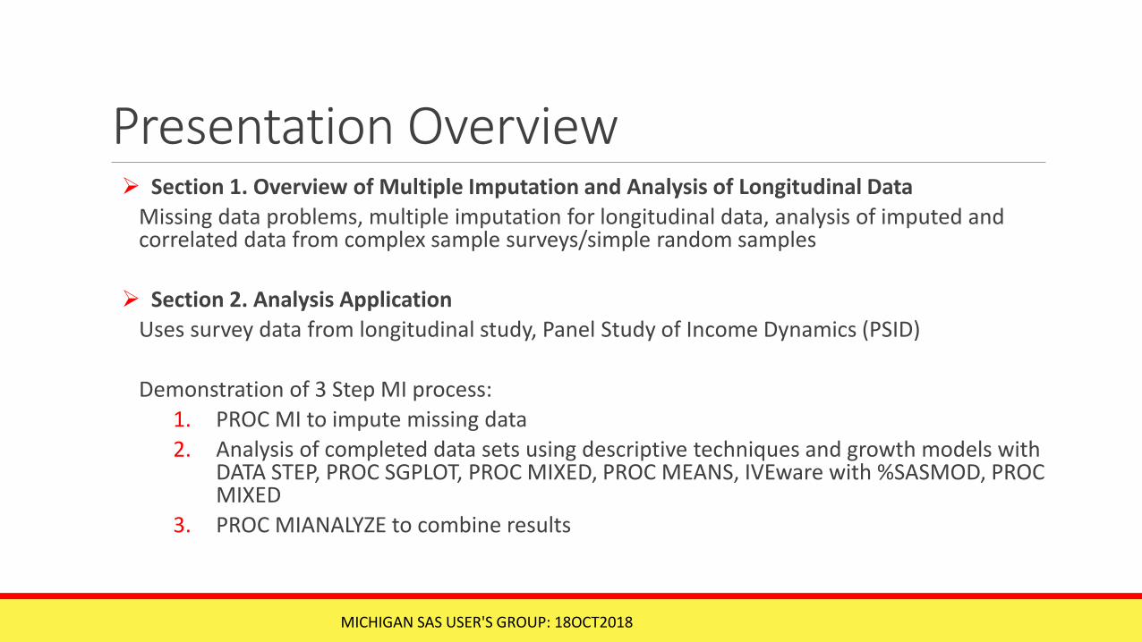
Presentation Overview Section 1. Overview of Multiple Imputation and Analysis of Longitudinal Data

Missing data problems, multiple imputation for longitudinal data, analysis of imputed and correlated data from complex sample surveys/simple random samples

Section 2. Analysis Application Uses survey data from longitudinal study, Panel Study of Income Dynamics (PSID)

Demonstration of 3 Step MI process:1. PROC MI to impute missing data 2. Analysis of completed data sets using descriptive techniques and growth models with

DATA STEP, PROC SGPLOT, PROC MIXED, PROC MEANS, IVEware with %SASMOD, PROC MIXED

3. PROC MIANALYZE to combine results


SECTION 1. OVERVIEW OF MULTIPLE IMPUTATION AND ANALYSIS OF LONGITUDINAL DATA


Handling Missing Data Missing data is everywhere, especially common in longitudinal data sets! What to do about

missing data?

Nothing - Complete case analysis usually default solution, loss of information can result in loss of analysis sample, not preferred approach

Simple Imputation -Univariate methods (mean, mode, etc.) popular but attenuate variances, do not account for increased variability due to imputation process, methods distort important distributional properties


Handling Missing Data, continued Multiple Imputation is 3 step process:

1. Impute missing data using PROC MI with appropriate model, fill in missing values to create M=X complete data sets

2. Analyze completed data sets using standard SAS procedures based on simple random sample assumption (PROC MEANS, PROC REG, PROC MIXED, etc.) or SURVEY procedures for complex sample data (PROC SURVEYMEANS, PROC SURVEYREG, etc.)

3. Combine analysis results using PROC MIANALYZE

Advantages of Multiple Imputation:˃ Model-based methods used to produce distribution of plausible values to replace

missing data values ˃ Accounts for variability introduced by imputation process itself


Characteristics of Missing Data Reasons for missing data - Structure of survey, file matching, refusal to answer, etc. Type of missing data - Item v. Unit, item missing data topic here, unit generally handled by

weighting adjustments

Assumptions – Missing at Random (MAR=default assumption of PROC MI/PROC MIANALYZE), Missing Completely at Random, Missing Not at Random Types of variables imputed - Continuous, nominal, binary, ordinal, count/mixed Missing data patterns - Arbitrary, monotone

Amount of missing information - Extent of missing information important factor when selecting M=(number of imputations)


Planning for Multiple Imputation Table 1 includes a suggested checklist for planning imputation session


MI Methods for Longitudinal Data Planning for imputation

˃ All planning and evaluative steps presented in previous slides apply to any imputation process but method differs from cross-sectional data imputation due to need to account for multiple waves of data

One popular method is called “Just Another Variable” (JAV), detailed by Raghunathan (2016) ˃ Method is used in today’s presentation

Another method is called “Two-Fold Fully Conditional Specification” (Welch et al, (2014) not demonstrated here)


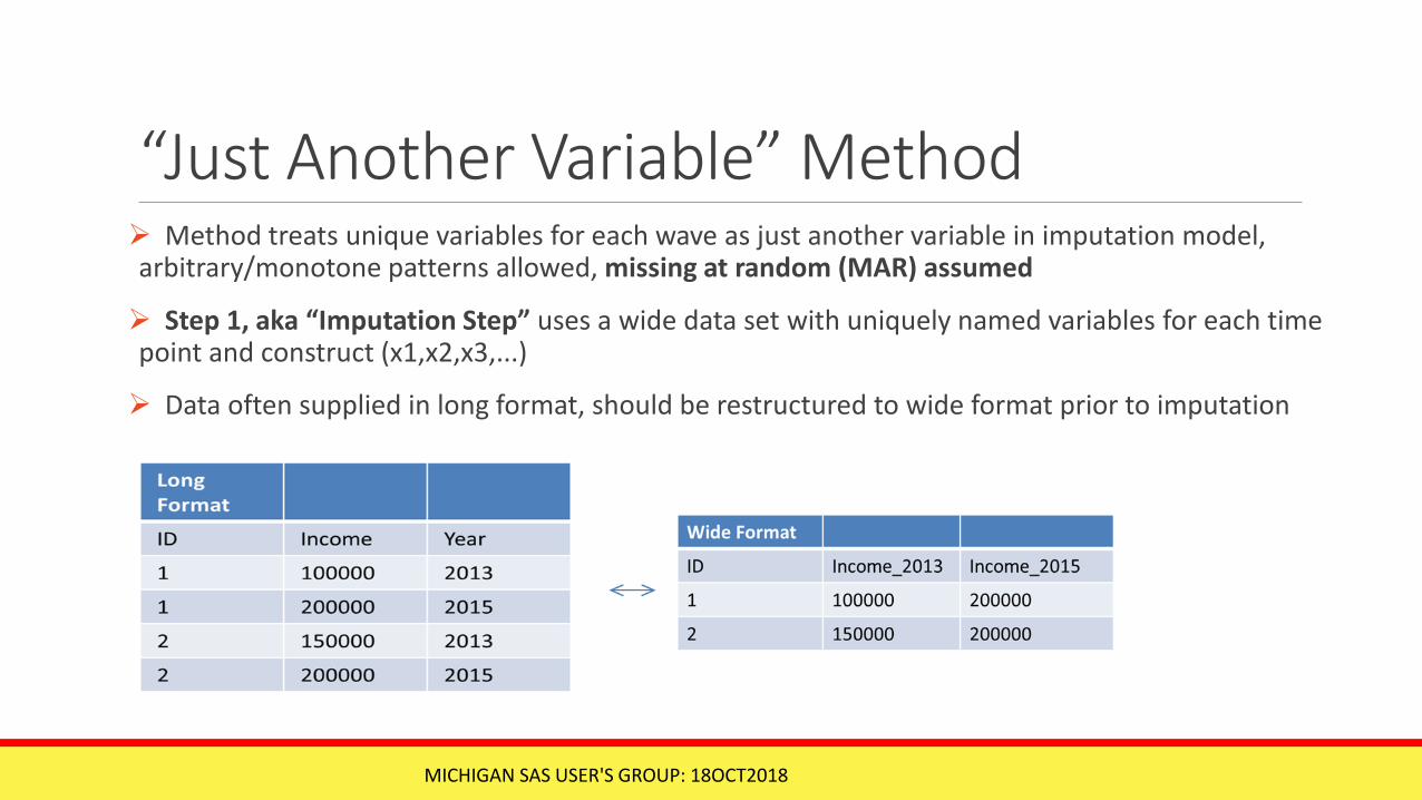
“Just Another Variable” Method Method treats unique variables for each wave as just another variable in imputation model, arbitrary/monotone patterns allowed, missing at random (MAR) assumed

Step 1, aka “Imputation Step” uses a wide data set with uniquely named variables for each time point and construct (x1,x2,x3,...)

Data often supplied in long format, should be restructured to wide format prior to imputation


“Just Another Variable” Method, Continued MI Step 2, aka “Analysis Step” uses completed data in long format with appropriate analysis

˃ Mixed Models or Repeated Measures models (PROC MIXED, PROC NLMIXED, PROC GENMOD, etc.) for panel data

MI Step 3, aka “Combining Step” uses Rubin’s rules (1987) for combining MI results ˃ Incorporation of increased variability due to imputation and repeated measures common in longitudinal data

JAV Method lacks way to capture individual changes across time yet is easily implemented in PROC MI, widely used in practice for all types of variables, easy to change data structures needed for method, highlighted in analysis application from Section 2


“Two-Fold FCS” Method Two-Fold Fully Conditional Specification (FCS) method performs multiple imputation as outlined in figure below adapted from Nevalainen, et al. (2009):

1. Within each wave (up/down arrows around each box in figure below) , 2. Across waves using specified t +/- (k) using iterative process (horizontal arrows across top and bottom of figure)

Method incorporates impact of responses at time t and those around t by using t-k and t+k, where k is typically 1 or 2 (specified by analyst)


“Two-Fold FCS” Method, Continued MI Steps 2 and 3 similar to those using JAV method, use appropriate analytic technique for longitudinal data analysis in Step 2 and correct combining rules for Step 3

Expectation is results are similar to those from JAV method when a relatively small number of waves and variables are used

For comparison of methods, see De Silva et al, (2017)



SECTION 2. ANALYSIS APPLICATION

DEMONSTRATION OF MULTIPLE IMPUTATION AND ANALYSIS OF LONGITUDINAL SURVEY DATA FROM THE PANEL STUDY OF INCOME DYNAMICS (PSID)

Overview of Analysis Application Introduction to PROC MI and PROC MIANALYZE Data from Panel Study of Income Dynamics (PSID)

Website is https://psidonline.isr.umich.edu/, long-running longitudinal study of U.S. families, 1968 to present, data downloaded from PSID data center

Use of descriptive techniques and growth models to analyze head’s wages/salary over time (1997-2013, odd years) by completed college status (completed grade 16+ in US education system), incorporates multiply imputed data in all analyses Data management to prepare data set including filters:

Individuals must be a head in each year, 1997-2013 and,

From Survey Research Center (SRC) or U.S. Census (Census) samples from 1968 and,

Head must be present in family in each year of series,

Final n=2,267 individuals.


https://psidonline.isr.umich.edu/

Overview of Analysis Application, continued Data management prior to imputation/analysis:

Data set in multivariate or wide format, no need to restructure for imputation Return previously imputed values (by PSID staff using modified Hotdeck method) back to missing for this application

Create new variables for imputation:Natural log of head’s wages/salary to address non-normal wage distributions Combined Strata and SECU variable for use as predictor in imputation models (along with longitudinal weight for 2013), see Berglund and Heeringa (2014) for more on imputation of complex sample data Refer to PSID documentation regarding weights and complex sample and related design variables Imputed value flag variables for some variables to assist in diagnostics


Introduction to PROC MI and PROC MIANALYZE PROC MI imputes missing data, offers a number of imputation methods and models:

“The MI procedure is a multiple imputation procedure that creates multiply imputed data sets for incomplete p-dimensional multivariate data. It uses methods that incorporate appropriate variability across the m imputations. The imputation method of choice depends on the patterns of missingness in the data and the type of the imputed variable.” (SAS 9.4 documentation)

PROC MIANALYZE combines results from MI step 1 (imputation) and step 2 (analysis of completed data sets):

“The MIANALYZE procedure combines the results of the analyses of imputations and generates valid statistical inferences. Multiple imputation provides a useful strategy for analyzing data sets with missing values.” (SAS 9.4 documentation)

Application shows both procedures plus more in action!


Summary of Analysis Variables Table 2 presents variables used in multiple imputation and analyses

Contents of Final MI Data Set (Wide Format)

Er32000 - Gender (1=M, 2=F), fully observed

Age1-Age9 - Age in 1997, 1999, 2001, 2003, 2005, 2007, 2009, 2011, 2013, fully observed

Strat_psu – Combined stratum and SECU (PSU) variable, fully observed, used to incorporate complex sample design features in imputation models

Er34268 – Probability weight from 2013, fully observed

Ed1-Ed9 – Highest grade completed (odd years 1997- 2013), missing data on each variable

Loghdwg1-Loghdwg9 – Log of head’s wages/salary (odd years 1997-2013), missing data on each variable

ID – ID68 and Person number combined to create unique individual indentifier, fully observed

Samplecat – Sample indicator of SRC or Census (1968 original sample), fully observed

Table 2. Contents of Final Analysis Data Set


3 Step Multiple Imputation Process Step 1. Multiple Imputation with PROC MI

Evaluate missing data problem, impute missing data separately within SRC and Census samples Perform imputation diagnostics and adjust imputations, if needed, before analysis of completed data setsRe-structure imputed data sets into long format suitable for longitudinal data analysis

Step 2. Analysis of Completed Data Sets using Appropriate ProceduresAnalyze complete data sets using descriptive and regression analyses (PROC MEANS and PROC MIXED), graph results (PROC SGPLOT)

Step 3. Combine Results using PROC MIANALYZE Combine results from MI Step 2, use output data from PROC MIANALYZE to generate tables and plotsAlternative: Use IVEware %SASMOD command with Jackknife Repeated Replication (IVEware is set of free SAS macros available from iveware.org) to repeat Example 2 using combining rules with complex sample variance estimation, See Appendix B of paper for example


Step 1 - Evaluation of Missing Data Problem Step 1 includes preliminary tasks - first evaluate the extent of missing data, types of variables with missing data, and missing data pattern in analysis data set

Code below uses PROC MI (NIMPUTE=0) and PROC MEANS with selected options on the procedure statement:

proc means data=w.psid1 n nmiss mean min max ;var er32000 age1-age9 strat_psu er34268 ed1-ed9 loghdwg1-loghdwg9 ;

run ;

proc mi data=w.psid1 nimpute=0 ;var er32000 age1-age9 strat_psu er34268 ed1-ed9 loghdwg1-loghdwg9 ;

run ;


Evaluation of Missing Data Problem, Continued Figure 4 indicates missing data on both education (ED1-ED9) and log head’s wages/salary (LOGHDWG1-LOGHDWG9), type of variables that require imputation, (binary, ordinal, continuous, nominal, etc.)

Education represents highest grade completed (1997-2013) with range of 3-17, Natural log of head’s wages (1996-2012) represents previous year wages, range from 0 (did not receive wage/salary in dollars for a given year) to 15.06 on log scale

Noted: log-transformed variables can produce bias and heavy tails in the distribution of the back-transformed, imputed version, recent research has demonstrated that for regression estimates, this bias is often mild, von Hippel (2013)

Caution: age and time are linked, if age is used as a predictor, should be treated as time-invariant, e.g., age at a fixed point such as age in 1997

Figure 4. Results from PROC MEANS


Evaluation of Missing Data Problem, Continued Figure 5 contains partial output from PROC MI (NIMPUTE=0), 4 of 128 missing data patterns shown:

Grid of frequency counts and percentages for observed data (“X”) and missing data (“.”) for each variable on VAR statement Group 1 is fully observed on all variables: 80.06% of sample or 1815 individuals assigned to the complete data group, full grid has 128 unique missing data patterns, one with all fully observed and the rest with <= 1.5% missing data Data has an arbitrary missing data pattern with continuous variables that require imputation

Figure 5. Results from PROC MI


Step 1 - Multiple Imputation of Missing Data PROC MI code:

˃ SEED=2017, NIMPUTE=10 , ROUND= (set imputed values to original scale (1) or to .01)˃ BY statement to impute within samples separately˃ CLASS statement to declare ER32000 (gender) and STRAT_PSU (combined Strata and SECU) as categorical ˃ FCS (Fully Conditional Specification) with NBITER=20 (requests 20 burn-in iterations) ˃ REGPMM with K=8 (8 closest neighbors) requests Predictive Mean Matching method for imputation models ˃ PLOT=TRACE to request trace plots for log of head’s wages for each of 9 waves (imputation diagnostic tool) ˃ VAR statement lists variables used in imputation

proc mi data=w.psid1 seed=2017 nimpute=10 out=impute_psid_mi

round= . . . . . . . . . . . . 1 1 1 1 1 1 1 1 1 .01 .01 .01 .01 .01 .01 .01 .01 .01 ;

by samplecat ;

class er32000 strat_psu ;

fcs nbiter=20 regpmm(ed1-ed9 / k=8 ) ;

fcs nbiter=20 plots=trace regpmm(loghdwg1-loghdwg9 / k=8 );

var er32000 age1-age9 strat_psu er34268 ed1-ed9 loghdwg1-loghdwg9 ;

run;


Multiple Imputation Diagnostic Plots Trace plots available from PROC MI with ODS GRAPHICS, excellent imputation diagnostic tool, shows imputed mean value by iteration separately by Sample

L ook for random patterns across the iterations for each line in Trace plot, lack of distinct pattern indicates lack of imputation problems, no obvious problems with mean values of imputations of Head’s wages/salary in 2004

Figure 6. Trace Plot of Head’s Wages/Salary 2004, SRC Sample Figure 7. Trace Plot of Head’s Wages/Salary 2004, Census Sample


Multiple Imputation Diagnostic Tables

===========================

Evaluate imputations with PROC MEANS, check mean wages by Sample, imputation number, and imputation indicator

Figure 8 (shows 4 of 10 imputations) reveals no apparent problems between observed (imphdwg1=0) versus imputed (imphdwg1=1) mean log wages in 1996, be sure to evaluate all imputations in a real-world situation

proc means data=impute_psid_mi;class samplecat _imputation_ imphdwg1;

var loghdwg1;run;

Figure 8. Mean Head’s Wages/Salary 1996 by Sample, Imputation, and Imputed Status


Step 1 - Convert Completed Data from Wide to Long Prior to analysis of completed data sets, restructure data set from wide to long format:

10 imputations*2,267 individuals*9 time points=204,030 records

DATA STEP code (next slide) uses arrays with iterative DO loop/OUTPUT statement to produce multiple records per individual file with back-transformation of log head’s wages/salary and conversion to 2013 dollars


Convert Data, continued


Review of Analysis Examples Explore trends in head’s wages/salary over time by college graduation status, descriptive and regression techniques used to address this goal Descriptive analysis focuses on mean head’s wages/salary by year and college graduation status, uses imputed data set from MI step 1 as input Growth models account for within and between-subject variation, predicted head’s wages/salary (based on mixed model results) calculated in the DATA STEP and plotted, uses imputed data set from MI step 1 as input

Additional Notes: MI Step 2 uses standard SAS procedures (SRS assumption) demonstrated but Appendix B shows a repeat of

Analysis Example 2 using PROC MIXED within the SASMOD framework of IVEware IVEware (iveware.org) implements Taylor Series Linearization and Jackknife Repeated Replication for design-

based variance estimates plus correct MI combining rules in one step, this complexity is needed to correctly analyze MI complex sample data

Analyses do not use differential weights in mixed models, not currently available in PROC MIXED but can be done in PROC GLIMMIX, see SAS/STAT PROC GLIMMIX documentation.


Analysis Example 1 - Wages/Salary by Year and College Graduation Status

Step 2. Analysis of Completed Data Sets

MI Step 2 uses imputed data sets from MI Step1, performs descriptive analysis of head’s wages/salary by imputation, college graduation status, and year

PROC MEANS used to prepare summary statistics that are saved to an output data set for use in PROC MIANALYZE (SAS code is shown on next slide)


Analysis Example 1 - Wages/Salary by Year and College Graduation Status, continued Example 1 uses PROC MEANS with BY and WEIGHT statements to obtain weighted means of head’s

wages/salary within each of 10 imputed data sets, by college status and time with OUTPUT statement to save statistics to file called “AVGWAGE”

Additional PROC SORT needed prior to combining using PROC MIANALYZE:

proc sort data=w.long_imputed ;

by _imputation_ collegegrad time ;

run ;

proc means data=w.long_imputed mean stderr ;

by _imputation_ collegegrad time ;

var headwage ;

weight er34268 ;

output out=avgwage mean=mean_headwage stderr=se_headwage ;

run ;

proc sort data=avgwage ;

by collegegrad time _imputation_ ;

run ;


Analysis Example 1 - Wages/Salary by Year and College Graduation Status, Continued Step 3. Combine Results

PROC MIANALYZE combines results from MI Step 2, generates variances that account for the additional variability introduced by MI

Combined estimates are mean wages/salary over time by college graduation status

BY statement used to produce combined estimates by college status and time

MEAN_HEADWAGE is MODELEFFECTS variable, SE_HEADWAGE is STDERR variable, ODS OUTPUT saves output data set with combined parameter estimates for use in PROC SGPLOT

PROC SGPLOT uses output file from PROC MIANALYZE with SERIES, XAXIS, YAXIS, and FORMAT statements for Figure 9 (next slide)


Mean Wages/Salary by College Graduate Status, 1997-2013


Plot shows trends over time for college graduates v. non-graduates, suggests possible interaction between Year (Time) and Completed College status

For college graduates, mix of positive and sharp negative slopes, for non-college graduates, slopes are flatter/smaller and primarily negative

Shows trends as household heads aged and experienced a changing economic climate during 1997-2013 and a wage differential of about $33,000

Figure 9. Mean Head’s Wages/Salary by College Graduate Status

Analysis Example 2 – Growth Model Step 2. Analysis of Completed Data Sets

Example 2 demonstrates use of growth model to investigate impact of time and college graduation status on head’s wages/salary

Model accounts for between-subject (intercept) and within-subject (time) variation by requesting random intercepts and slopes

Time treated as continuous rather than categorical predictor in model


Model Fitting Prior to Inference Prior to inference step (Step 4), model fitting performed using Steps 1-3 recommended by the SAS Institute “Mixed Model Analyses of Repeated Measures Data” course notes (Steps 1-3 not shown in this presentation):

Step 1- Model mean structure, specify fixed effects Step 2- Set covariance structure for within-subject and/or between-subject effectsStep 3- Use Generalized Least Squares (GLS) to fit mean model with selected covariance structureStep 4- Make statistical inference based on model from Step 3, aim for parsimonious model

Steps 1-3 done separately within M=10 imputed data sets to test 3 covariance structures:Unstructured (UN), Auto-Regressive (AR(1)), Toeplitz with PROC MIANALYZE used for combining results

Evaluation of AIC and BIC statistics for 3 structures tested, use Unstructured (UN)


Analysis Example 2 - Growth Model Step 2. Analysis of Completed Data Sets PROC MIXED with options:

BY _IMPUTATION_ executes model separately for 10 imputed data sets CLASS statement with COLLEGEGRAD and ID treated as categorical MODEL statement with HEADWAGE regressed on TIME (continuous), COLLEGEGRAD, and TIME*COLLGEGRAD, SOLUTION for fixed effects, DDFM=BW for between-within method for denominator degrees of freedom RANDOM INTERCEPT TIME / TYPE=UN SUBJECT=ID to request random intercept/slopes with unstructured covariance, subject is ID variable WEIGHT statement declares PSID 2013 longitudinal weight (last year studied) ER34268 as weight variable ODS OUTPUT outputs data set of parameter estimates needed for PROC MIANALYZE PROC PRINT displays data set, OUTCOMBINE_RANDOM (see Table 3 on next slide):

proc mixed data=w.long_imputed noclprint; by _imputation_; class collegegrad id; model headwage = time collegegrad time*collegegrad / solution ddfm=bw; random intercept time / type=un subject=id; weight er34268; ods output solutionf=outcombine_random; run;proc print data=outcombine_random;run;


Analysis Example 2 - Growth Model, Continued

Table 3 displays fixed effects estimates, standard errors, degrees of freedom, tvalues, and p values for 2 of 10 imputed data sets

Estimates and statistics are slightly different for each imputed data set, reflecting the differing imputed values


_Imputation_ Effect collegegrad Estimate StdErr DF tValue Probt

1 Intercept _ 71300 2530.22 2266 28.18 <.0001

1 time _ -1649.66 443.64 18E3 -3.72 0.0002

1 collegegrad 0 -29708 3009.02 156 -9.87 <.0001

1 collegegrad 1 0 . . . .

1 time*collegegrad 0 913.39 524.87 18E3 1.74 0.0818

1 time*collegegrad 1 0 . . . .

2 Intercept _ 71764 2558.86 2266 28.05 <.0001

2 time _ -1696.62 447.75 18E3 -3.79 0.0002

2 collegegrad 0 -29651 3044.51 153 -9.74 <.0001

2 collegegrad 1 0 . . . .

2 time*collegegrad 0 873.99 530.78 18E3 1.65 0.0997

2 time*collegegrad 1 0 . . . .

Table 3. Print-Out of Fixed Effects Parameters for 2 of 10 Imputed Data Sets

Analysis Example 2 - Growth Model, Continued Step 3. Combine Results PROC MIANALYZE used to combine results from MI Step 2:

DATA=OUTCOMBINE_RANDOM reads data produced in Step 2PARMS(CLASSVAR=FULL) statement declares full set of discrete levels for the CLASS variablesCLASS statement uses COLLEGEGRAD as a categorical variableMODELEFFECTS specifies model intercept and predictor variables (same order as in Step 2)ODS OUTPUT creates data set of estimates called OUTCOMBINE_RANDOM_APROC PRINT produces a listing of the contents of the final output data set (see next slide):

proc mianalyze parms(classvar=full)=outcombine_random; class collegegrad; modeleffects intercept time collegegrad time*collegegrad; ods output parameterestimates=outcombine_random_a; run; proc print noobs data=outcombine_random_a;var parm collegegrad estimate stderr tvalue probt; run;




Parameter College Graduate Estimate MI SE T Value P value

intercept . 71442.00 2553.67 27.98 <.0001

time . -1678.08 447.16 -3.75 0.0002

collegegrad 0 -29798.00 3027.97 -9.84 <.0001

collegegrad 1.000000 0 . . .

time*collegegrad 0 924.72 529.55 1.75 0.0808

time*collegegrad 1.000000 0 . . .

Table 4. Combined Parameter Estimates for Growth Model

Table 4 presents combined (PROC MIANALYZE) parameter estimates, MI standard errors, with t and p values

Growth model estimates account for between-subject (intercept) and within-subject (time) variation through use of the RANDOM statement

Based on Table 4 results, time, college graduation status and their interaction are all significant at the alpha=0.10 level , time and college status are also significant at the alpha=0.05 level, interaction term is nearly significant at the 0.05 level, remains in model for demonstration purposes



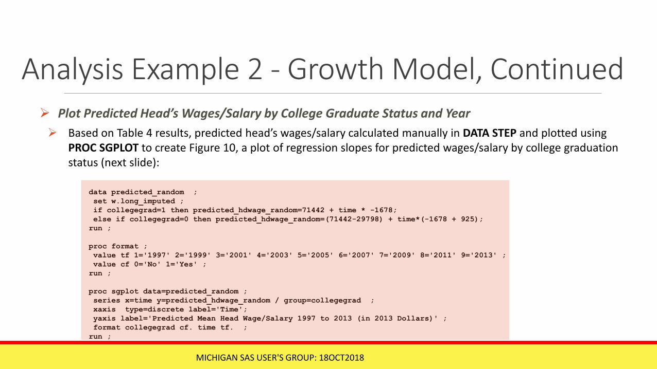
Plot Predicted Head’s Wages/Salary by College Graduate Status and Year Based on Table 4 results, predicted head’s wages/salary calculated manually in DATA STEP and plotted using

PROC SGPLOT to create Figure 10, a plot of regression slopes for predicted wages/salary by college graduation status (next slide):

data predicted_random ; set w.long_imputed ; if collegegrad=1 then predicted_hdwage_random=71442 + time * -1678; else if collegegrad=0 then predicted_hdwage_random=(71442-29798) + time*(-1678 + 925); run ;

proc format ; value tf 1='1997' 2='1999' 3='2001' 4='2003' 5='2005' 6='2007' 7='2009' 8='2011' 9='2013' ; value cf 0='No' 1='Yes' ; run ;

proc sgplot data=predicted_random ; series x=time y=predicted_hdwage_random / group=collegegrad ; xaxis type=discrete label='Time'; yaxis label='Predicted Mean Head Wage/Salary 1997 to 2013 (in 2013 Dollars)' ; format collegegrad cf. time tf. ; run ;


Figure 10. Growth Model Results

Figure 10 presents regression lines of predicted head’s wages/salary (odd yrs, 1997-2013) by college graduate status

Negative slope (head’s wages/salary in 2013 dollars) for college graduates is steeper than for non-graduates, intercepts are estimated to be about $30,000 lower for non-graduates

Though non-graduates have flatter slope, income over time is lower than college graduates, reflecting head’s wage/salary differences between levels of education during 1997-2013

Reminder, results derived from analysis that does not incorporate the complex sample design features but does adjust for Multiple Imputation variance


Analysis Example 2 – Growth Model Repeated, IVEware %SASMOD and PROC MIXED

Parameter College Graduate Estimate

IVEware SE (Design-Based and MI Estimation)

Wald Test p Value

Intercept . 71442.00 2559.09 1203.79 0.00000

Time . -1678.08 400.44 17.56 0.00003

Collegegrad 0 -29798.00 2088.85 203.49 0.00000

Collegegrad 1.00 0 . . .

Time*Collegegrad 0 924.72 510.78 3.28 0.07023

Time*Collegegrad 1.00 0 . . .

Table 4a presents combined (from IVEware SASMOD/PROC MIXED) parameter estimates with design-based and MI standard errors, Wald tests and p values

Based on Table 4a, time, college graduation status and their interaction are all still significant at the alpha=0.10 level , time and college status are also significant at the alpha=0.05 level

Using complex sample and MI variance estimation changes the SE’s/related statistics but does not change overall conclusions in this example

Generally, survey data analysts should account for complex sample features and MI in variance estimation

Table 4a. Growth Model Results Using IVEware


Summary of Presentation Topics Discussion of missing data issues in longitudinal data, two potential imputation methods appropriate

for panel data, and use of multiple imputation using the JAV method

Analysis application uses PSID longitudinal data to study wages/salary trends as US household heads age over the years 1997-2013

Detailed presentation of MI 3 Step process: 1) PROC MI to perform multiple imputation in correct data structure

2) Analysis of completed data sets using growth models (PROC MIXED/PROC SGPLOT) and descriptive techniques (PROC MEANS/PROC SGPLOT)

3) Combine analyses of imputed data sets using PROC MIANALYZE

Detailed examples of descriptive techniques and growth models to explore wages/salary trends over time, while accounting for variability introduced by multiple imputation process


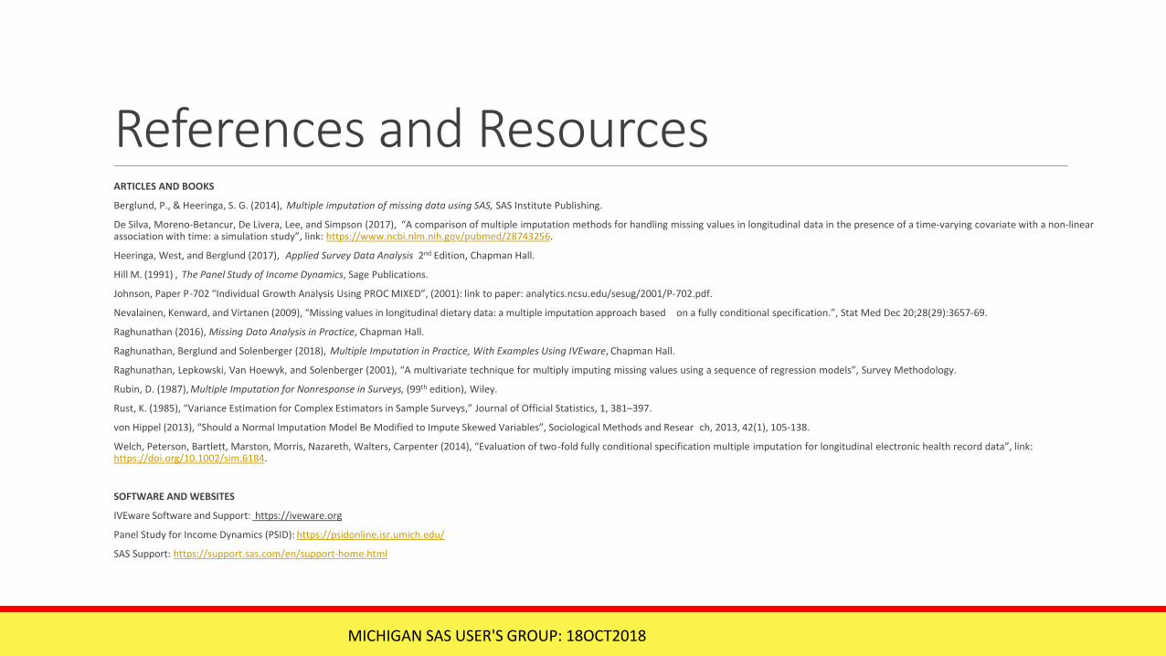
References and ResourcesARTICLES AND BOOKS

Berglund, P., & Heeringa, S. G. (2014), Multiple imputation of missing data using SAS, SAS Institute Publishing.

De Silva, Moreno-Betancur, De Livera, Lee, and Simpson (2017), “A comparison of multiple imputation methods for handling missing values in longitudinal data in the presence of a time-varying covariate with a non-linear association with time: a simulation study”, link: https://www.ncbi.nlm.nih.gov/pubmed/28743256.

Heeringa, West, and Berglund (2017), Applied Survey Data Analysis 2nd Edition, Chapman Hall.

Hill M. (1991) , The Panel Study of Income Dynamics, Sage Publications.

Johnson, Paper P-702 “Individual Growth Analysis Using PROC MIXED”, (2001): link to paper: analytics.ncsu.edu/sesug/2001/P-702.pdf.

Nevalainen, Kenward, and Virtanen (2009), “Missing values in longitudinal dietary data: a multiple imputation approach based on a fully conditional specification.”, Stat Med Dec 20;28(29):3657-69.

Raghunathan (2016), Missing Data Analysis in Practice, Chapman Hall.

Raghunathan, Berglund and Solenberger (2018), Multiple Imputation in Practice, With Examples Using IVEware, Chapman Hall.

Raghunathan, Lepkowski, Van Hoewyk, and Solenberger (2001), “A multivariate technique for multiply imputing missing values using a sequence of regression models”, Survey Methodology.

Rubin, D. (1987), Multiple Imputation for Nonresponse in Surveys, (99th edition), Wiley.

Rust, K. (1985), “Variance Estimation for Complex Estimators in Sample Surveys,” Journal of Official Statistics, 1, 381–397.

von Hippel (2013), “Should a Normal Imputation Model Be Modified to Impute Skewed Variables”, Sociological Methods and Resear ch, 2013, 42(1), 105-138.

Welch, Peterson, Bartlett, Marston, Morris, Nazareth, Walters, Carpenter (2014), “Evaluation of two-fold fully conditional specification multiple imputation for longitudinal electronic health record data”, link: https://doi.org/10.1002/sim.6184.

SOFTWARE AND WEBSITES

IVEware Software and Support: https://iveware.org

Panel Study for Income Dynamics (PSID): https://psidonline.isr.umich.edu/

SAS Support: https://support.sas.com/en/support-home.html


https://www.ncbi.nlm.nih.gov/pubmed/28743256

https://doi.org/10.1002/sim.6184

https://psidonline.isr.umich.edu/

https://support.sas.com/en/support-home.html

Contact InformationThank you for attending.

Your comments and suggestions are welcome!

Patricia A. Berglund

Institute for Social Research – University of Michigan

E-Mail: [email protected]


Presenter Information - Michigan SAS Users Group Home Page · Handling Missing Data, continued...

Documents

Transcript of Presenter Information - Michigan SAS Users Group Home Page · Handling Missing Data, continued...