Presented on July 29, 1981 Title: MODIFICATIONS OF STATIC ...

AN ABSTRACT OF THE THESIS OF

Kevin John Boyle for the degree of Master of Science

in the Department of Agricultural and Resource Economics

Presented on July 29, 1981

Title: MODIFICATIONS OF STATIC INPUT-OUTPUT MODELS TO REFLECT

SECTORAL CHANGE

Abstract approved: .(,— ,.—Ly .^.-n,. ■

Frederick W. Obermiller

Input-output models have been used for many years and have been

applied to a variety of problems. These models typically are used in

economic planning and impact assessment. In a purely descriptive

sense, an input-output model enhances one's understanding of an eco-

nomy.

Although input-output models are commonly used as an economic

tool, these models do become outdated over time. The most common

source of obsolescence is reflected in the structural coefficients,

i.e., the purchasing patterns of sectors within an economy may change.

There are several procedures for updating models to account for such

changes. The location of a new industry (sector) within the modeled

economy also results in the need to update a model. In this case,

the model must be expanded to incorporate the new sector.

The present research develops an ex-ante method for incorporating

a new sector into an input-output model. The ex-ante procedure is

applied by incorporating a new sector (coal fired power plant) into

the Morrow County (Oregon) input-output model. Implications of the

existence of excess capacity in the Morrow County economy are evaluated.

It is concluded that the ex-ante procedure may lead to questionable

results when projected increases in sales exceed a sector's excess ca-

pacity. Two of the basic assumptions of input-output analysis may be

violated: constant structural coefficients and perfectly elastic

supply. In other words, the economy may not be able to adjust per-

fectly and instantaneously to the projected interindustry transactions

of the new sector.

The ex-ante procedure developed for the present research requires

further evaluation. An ex-post analysis would.give some indication as

to whether the assumptions underlying static input-output analysis,

as noted above, are indeed violated when projected sales exceed ex-

cess capacity. However, ex-post analysis may not provide a definite

answer. It is important to realize that an economy changes through

time; thus, there will be other variables acting on the economy in the

interim.

The ex-ante procedure used here implicitly assumes that there is

a demand for the new sector's product. This assumption may be rea-

sonable when a new sector has already made a decision to locate (e.g.,

the coal fired power plant in Morrow County), but may not be reasonable

when such a decision has not been made. In short, the procedure makes

no assumptions about the feasibility of the industrial location de-

cision.

MODIFICATIONS OF STATIC INPUT-OUTPUT MODELS

TO REFLECT SECTORAL CHANGE

by

Kevin J. Boyle

A THESIS

submitted to

Oregon State University

in partial fulfillment of the requirements for the

degree of

Master of Science

Completed July 29, 1981

Commencement June 1982

APPROVED:

Associate Professor of Agricultural and Resource Economics in charge of major

Head of Agricultural and Resource Economics

Gradu/tje School jT" Dean of

Date thesis is presented July 29, 1981

Typed by Nina M. Zerba for Kevin John Boyle

ACKNOWLEDGEMENTS

My sincere thanks to the following:

Dr. Frederick Obermiller

Dr. Charles Vars

Nancy Becraft

Hermine - my dog

Nina Zerba

Linda Eppley

Vivian Ledeboer

David Lambert

Interviewers for the input-output model

TABLE OF CONTENTS

I. Introduction 1

Study Area 2

The Problem 4

Objectives 6

Study Organization 6

II. The Theory and Methods of Input-Output Analysis ... 9

Historical Perspective 9

Development of a Theoretical Input-Output Model 11

Differences Between the Leontief Model and the Keynesian Model 13

Distinction Between Input-Output Economics and Inter-Industry Economics 15

Assumptions of Input-Output Analysis ... 16

Transactions Table 19

Direct Coefficients 24

Direct Plus Indirect Coefficients 26

Multipliers 29

Concluding Remarks 30

III. The Morrow County Input-Output Model 32

Sector Specification 32

Sample Selection 35

Survey Procedures and Results 37

Study Results '. 40

Transactions Table 40

Direct Coefficients 50

Direct Plus Indirect Coefficients 51


IV. Introducing a New Sector into a Static Input-Output Model: An Ex-ante Procedure 57

Review of the Literature 59

Procedures and Assumptions for Incorporating a New Sector 60

Introducing the Coal Fired Power Plant into the Morrow County Input-Output Model 67

Incorporating the New Sector 67

The Effect of the Coal Fired Power Plant on Sales 69

The Effect of the Coal Fired Power Plant on Employment 71

Structural Change 73

Evaluating the Validity of the Ex-ante Procedure. . 75

Excess Capacity 75

Employment 79

Simulating the Coal Fired Power Plant with Endogenous Sales 80


V. Summaries and Conclusions 84

The Objectives .84

Summary 84

Conclusions 86

Implications for Future Research 89


Bibliography 93

Appendix A. Morrow County Input-Output Survey Forms and Explanatory Letters 97

Guide to Contents 98

Appendix B. A Procedure for Developing Expansion Coefficients to Project Population Estimates of Inter-industry Trans- actions 136

Development of Expansion Coefficients . . . . . . . 137

Appendix C. Input-Output Tables Without the Coal Fired Power Plant Sector 141

Table C-l. Transactions Table Without the Coal Fired Power Plant Sector, 1979 ($1,000) 142

Table C-2. Matrix of Direct Coefficients Without the Coal Fired Power Plant Sector, 1979 143

Table C-3. Matrix of Direct Plus Indirect Coefficients Without the Coal Fired Power Plant Sector, 1979 144

Appendix D. Input-Output Tables with the Coal Fired Power Plant Sector 145

Table D-l. Transactions Table with the Coal Fired Power Plant Sector in 1979 Dollars C$1,000) 146

Table D-2. Matrix of Direct Plus Indirect Coefficients with the Coal Fired Power Plant Sector 147

Appendix E. Estimation of Employment Multipliers 148

Estimation Procedure 149

Application 150

Table E-l. Results of Regressing Employment on Total Sales, by Sector 152

Table E-2. Employment Multipliers for the Morrow County Input-Output Model, by Sector 153

Appendix F. Matrix of Direct Plus Indirect Coefficients Simulating the Coal Fired Power Plant with Endogenous Sales . . 154

Table F-l. Matrix of Direct Plus Indirect Coefficients Simulating the Coal Fired Power Plant with Endogenous Sales 155

LIST OF FIGURES

Figure Page

I Map of Morrow County 3

II Fixed Factor Proportion Isoquant Map 18

LIST OF TABLES

Table Page

I A Hypothetical Transactions Table 20

II Sectors of the Morrow County Input-Output Model (without the CFPP Sector) 34

III Sampling Information for Development of the Morrow County (Oregon) Input-Output Model 39

IV Expansion Coefficients for Projecting Morrow County Input-Output Population Values from the Sample Data . . 41

V Value of Total Output, Exports, and Imports Among Sectors of the Morrow County (Oregon) Economy in 1979 42

VI Morrow County Exports and Imports as a Percent of Sector Sales 44

VII Net Trade Balances Among Sectors of the Morrow County (Oregon) Economy in 1971 46

VIII Percentages of Purchases from Local Households by Sectors of the Morrow County (Oregon) Economy in 1979 . 48

IX Sectors with Greater than Five Percent of Purchases Made from Nonlocal Households 49

X Output Multipliers of Each Sector of the Morrow County Input-Output Model 53

XI Contribution of Final Demand Sales by Each Sector of the Morrow County (Oregon) Economy to Total County Business Activity in 1979 55

XII Projected Purchasing and Selling Pattern of the Coal Fired Power Plant 68

XIII Direct Plus Indirect and Induced Increases in Sales of Endogenous Sectors 70

XIV Direct Plus Indirect Increases in Employment, by Sector 72

LIST OF TABLES (cont.)

Table Page

XV Column Coefficients for the Coal Fired Power Plant from the Matrix of Direct Coefficients 74

XVI Increased Sales and Excess Capacity (for 1979) in the Morrow County (Oregon) Economy, by Sector .... 78

XVII Row Coefficients for the CFPP Sector from the Inverse Matrices 82

CHAPTER I

MODIFICATIONS OF STATIC INPUT-OUTPUT MODELS TO REFLECT SECTORAL CHANGE

INTRODUCTION

In May, 1980, the Department of Agricultural and Resource Eco-

nomics (Oregon State University) entered into a contractual agreement

with the Morrow County Court to construct a primary data input-output

model of the Morrow County (Oregon) economy. More precisely, the

contract called for the development of an inter-industry model.

There were two major purposes for constructing the model. The first

objective was to document the county's dependency on basic resource-

using industries. The second objective was to develop a tool which

could be used for economic impact assessments at the county level.

The desire by Morrow County officials to have an inter-industry

model of the county economy was, in part, a direct result of the

rapid economic growth which the county has been experiencing in re-

cent years. During the period 1973 to 1978, Morrow County was the

second fastest growing county in the United States. The total growth

in personal income was 254 percent [U.S. Department of Commerce,

1980 (b)]. A major factor contributing to the growth of the Morrow

County economy was, and is, the expansion of irrigated agriculture

in the northern end of the county (see Figure 1). Irrigated acreage

increased from 12,500 acres in 1965 to an estimated 62,000 acres in

1980.

The growth in irrigated agriculture stimulated growth in other

sectors of the county economy. For example, a food processing plant

was constructed in Boardman (in 1975) in response to the growth in

potato production--a crop associated solely with sprinkler irrigation

systems first introduced in 1965. The plant initially had 162 full

time equivalent employees and has expanded its employment in subse-

quent years (Obermiller, 1975). The most recent industrial develop-

ment in Morrow County has been the construction of a coal-fired power

plant (CFPP) by Portland General Electric. This plant is located

just south of Boardman.

Accompanying the growth in irrigated agriculture and manufacturing

has been rapid population growth in Morrow County. During the period

1973 to 1978, the population of Morrow County grew by 54 percent.

This is in contrast to 11 and 4 percent increases for Oregon and the

United States, respectively. The population of Morrow County was 4,600

in 1973 and grew to 7,100 in 1978 [U.S. Department of Commerce, 1980

(a)].

Study Area

The geographical boundaries of Morrow County are the limits of

the county economy for purposes of the present study. This definition

was adopted for the logical reasons that the Morrow County Court pro-

vided funding for the development of the input-output model, and

in a geopolitical sense the county, in Oregon is an economic unit.

O County Seat

9 Incorporated Cities

Figure I. Map of Morrow County

Morrow County can be divided into two sections—north and south

(see Figure 1). The south end contains the county seat (Heppner), and

is the traditional business center of the southern half of the county.

The major income producing activities in the south end are dryland

wheat, cow-calf operations, and wood products. Dryland wheat and cow-

calf operations are the traditional forms of agriculture in the

county.

The north end is the recipient of the rapid growth which the

county recently has been experiencing. The growth initially was gene-

rated by an expansion in irrigated agriculture; as noted above. In

response to the growth in irrigated agriculture, the food processing

plant was constructed in Boardman. In turn, many new service indus-

tries opened in the community. The construction and operation of the

CFPP has provided an additional and continuing stimulus to growth in

the north end.

The Problem

The construction of the coal-fired power plant created a one-time

stimulus for the Morrow County economy; but, the operation of the plant

will have a prolonged effect on local economic activity. Morrow County

business leaders expected the inter-industry model to provide some

insight as to the effect of the operational CFPP on the local economy;

that is, the plant could be assumed to have a significant impact

through its interactions with established businesses within the county.

The above question (expectation) presented a problem in de-

veloping the Morrow County inter-industry model. The survey data

for the model was collected (in the summer of 1980) for the 1979 calen-

dar year. The power plant was not operating in 1979, and is not sched-

uled for on-line production until 1982. In addition, the CFPP did not

conform with the standard inter-industry sector definitions for any

of the existing sectors of the Morrow County economy. Thus, the ef-

fect of the plant's operation on the local economy could not be treated

as a change in final demand for an existing industry's (sector's) out-

put. Rather, the plant could only be treated as a distinctly new

sector in the inter-industry model.—

The process of establishing the coal-fired power plant as a new

sector in the Morrow County inter-industry model is not straight-

forward. The 1979 survey data did not contain observations of the

CFPP interactions with existing firms in the local economy, because

the plant was not operating in 1979. An ex-ante procedure was required

to incorporate the plant (new sector) into the model and to assess

its effects on the local economy. The development of an ex-ante

procedure for incorporating a new sector into an existing inter-

industry model, and the effect of the coal-fired power plant on the

Morrow County economy, are the topics addressed in this thesis.

— A one firm sector does not present disclosure problems in that the CFPP is owned by Portland General Electric which is a public utility.

Objectives

The objectives of the present study are as follows: 1) to con-

struct a static inter-industry model of Morrow County (Oregon); 2)

to develop an ex-ante procedure for incorporating a new sector into

an existing inter-industry model; 3) to examine the aggregative and

distributional effects which the CFPP would have on the Morrow County

economy; 4) to evaluate the effect which firms with transactions pat-

terns different from the CFPP might have on the county economy; and

5) to evaluate the extent to which the ex-ante procedure developed

for objective (2) is an adequate representation of reality.

Study Organization

In accomplishing the objectives presented above, a survey was

conducted of firms, households, and government agencies located within

Morrow County during the summer of 1980. Information was collected

on the selling and purchasing patterns of these units. As was noted

earlier, these observations were collected for the 1979 calendar year.

The survey was conducted via personal interviews with firms and go-

vernment agencies, and by mail survey for households. The data col-

lected through the survey process were used to develop an inter-

industry model of the Morrow County economy.

The third objective was accomplished by interviewing Portland

General Electric as to its projected purchases and sales from/to

7

both local and nonlocal economic sectors when the CFPP is fully

operational. The projected transactions data were converted to 1979

dollars and used, via the ex-ante procedure (second objective) pre-

sented in Chapter IV, to incorproate the CFPP as a new sector in the

model. The aggregative and distributional effects of the power plant

were evaluated using the new inter-industry model of Morrow County

(expanded to incorporate the CFPP sector). The impacts of the new

sector were calculated by examining changes in gross regional out-

put, total sales by sector, household income, and employment by

sector. Structural changes were evaluated by examining the inter-

industry tables with and without the CFPP sector.

The fourth objective addresses the effect which firms (sectors)

with different transaction patterns will have on the structure and

development of the Morrow County economy. This objective is ac-

complished by simulating the Jocal economic system as it might exist

with the CFPP making endogenous sales. (The CFPP will, in actuality,

only make exogenous sales when it is fully operational).

The validity of the ex-ante procedure for incorporating a new

sector is evaluated by examining the excess capacity existing in Morrow

County during the survey period (1979); that is, whether the increased

sales of local sectors, resulting from the introduction of the new

purchasing sector, exceed the existing sectors' excess capacities.

If capacity constraints are exceeded, it is questionable as to whether

the assumptions by which the ex-ante procedure is developed are appli-

cable. This discussion is developed further in Chapter IV.

The organization of the remainder of this thesis is as follows:

In the next chapter (Chapter II), the theory of input-output analysis

is reviewed. In Chapter III, the inter-industry model of Morrow

County, without the CFPP, is presented. The ex-ante procedure for

incorporating a new sector into an existing inter-industry model is

developed in Chapter IV. Chapter IV also contains the discussion of

the inter-industry model of Morrow County in which the local economy

with a CFPP making endogenous sales is simulated. Summaries and

conclusions with respect to the present study are offered in the

final chapter.

CHAPTER II

THE THEORY AND METHODS OF INPUT-OUTPUT ANALYSIS

Historical Perspective

Input-output analysis has been used as an economic tool for

many years. The origins of this type of economic analysis pre-

date the table of inter-industry relations developed by Leontief

in 1931. The Soviets published a table of inter-industry relations

for their economy in 1925. The first empirical application of input-

output analysis to the United States economy was by Leontief in

1936.

The basic concepts of input-output analysis and inter-industry

relations can be traced to Quesnay's "Tableau Economique" in 1758

and Walras' general equilibrium model of the 1870's. The theo-

retical framework of Leontiefs input-output model drew heavily on

Walras' model and, to a lesser degree, on the work of Pareto (Chenery

and Clark, 1959).

The Walras model specified a system of equations which would de-

termine all of the prices in an economy when solved simultaneously

(Miemyk, 1965). Each price in this system has its own equation.

Miemyk points out that the Walras model portrays the interdependence

of producing sectors of the economy and the competing demands of each

sector for factors of production. The system of equations represents.

10

in part, consumer income and expenditures and allows consumers to sub-

stitute purchases from one sector of the economy to another. The

model also takes into account the costs of production in each sector,

total demand for and supply of commodities, and supply and demand of

factors of production.

Miemyk (1965) noted that the Walras model is not empirically im-

plementable, even if sufficient data were available, due to the com-

plexity of the system of equations. Given the practical limitations

of the theoretical model, Leontief simplified the Walras model so

that the equations could be estimated empirically (Dorfman, 1954).

The simplification process involved two assumptions (Richardson,

1972):

1. The large number of commodities in the Walras model were aggregated into a relatively few outputs--one for each sector.

2. The equations for the supply of labor and final demand were not used, and the remaining production equations were expressed in their simplest form.

These assumptions artificially reduce the number of equations and

unknowns and allow the theoretical model to be empirically estimated.

Chenery and Clark (1959) noted that Leontief excluded the effects

of limited factor supplies but adopted Walras' assumption of fixed

production coefficients. Thus, Leontief eliminated the effect of

price on consumer demand, intermediate inputs, supply of labor, etc.

In turn, the Leontief model precludes many of the adjustments which

are characteristic of the Walrasian system.

11

In the Leontief model, supply and demand are equated by hori-

zontal shifts in the demand curve, given constant relative prices.

Supply is assumed to be perfectly elastic (Chenery and Clark, 1959).

Thus, supply and demand are equated by adjustments in production

levels, rather than by changes in price as would be experienced by

moving along the supply and demand curves. The Leontief system is

assumed to be in equilibrium at given prices (Richardson, 1972).

Development of a Theoretical Input-Output Model

The above assumptions can be used to develop an input-output

model that divides an economy into sectors based on the production

activities of the units which compose the economy. As noted above,

each sector produces one product (or many products which are perfect

2/ substitutes in consumption).— It is also assumed that each sector's

product(s) is (are) unique, and that all firms within a sector face

the same production function. Each sector in the model has a dis-

tinct production function (Chenery and Clark, 1959). The production

functions for each sector are assumed to demonstrate fixed factor pro-

portions (production coefficients) and are homogeneous of degree one

(Chenery and Clark, 1959; Richardson, 1972). Thus, input-output

2/ — If substitutes are aggregated into sectors, the input coef-

ficients will be unstable if the production processes composing the aggregate do not have similar input structures (Chenery and Clark, 1959).

12

analysis is based on the premise that it is possible to divide the

productive activities of an economy into sectors whose relations

are meaningful and can be expressed in simple input functions.

The division of an economy into sectors is used to facilitate

the description of the interactions of producing units in an economy;

that is, the flow of goods and services between producing and con-

suming sectors. Leontief states that input-output economics is

"... essentially a method of analysis that takes advantage of the

relatively stable pattern of the flow of goods and services among the

elements of our economy to bring a much more detailed statistical

picture of the system into the range of manipulation by economic

theory." (Leontief, 1966). Or, as Chenery and Clark (1959) have

stated:

"Since [input-output] analysis is concerned with interrelations arising from production, the main function of [input-output] accounts is to trace the flows of goods and services from one productive sector to another."

Thus, input-output analysis is a simplified procedure for viewing an

economy through empirical techniques.

As alluded to above, a distinction is drawn between sectors

located within an economy (endogenous) and sectors located outside

of an economy (exogenous). Endogenous sectors represent producing

units within the economy being modeled. Exogenous sectors represent

producing units located outside the economy being modeled, as well as

nonproduction accounting relationships, e.g., depreciation, investment,

net inventory change. The distinction between endogenous and

13

exogenous sectors is similar to the one drawn in the Keynesian model

between induced and autonomous elements of an economy (Chenery and

Clark, 1959). Hence, input-output models, as presented in this thesis

are static and emphasize current account transactions.

Differences Between the Leontief Model and the Keynesian Model

As was noted above, in certain respects the Leontief input-output

model is similar to the Keyneisan aggregate income model. This is not

always the case. For example, the traditional Leontief input-output

model treats households as an exogenous sector (Miemyk, 1965). This

is what is known as the "open Leontief model," but the Leontief model

3/ can also be closed with respect to household transactions.—

The "open Leontief model" conflicts with traditional Keynesian

economics (Bromley, 1967). In the open model, a consumption function

is irrelevant since consumption, which is part of final demand, is

independent of output, employment, and thus, income. Consumption is

thus determined exogenously from the model, i.e., in the Keynesian

notation it would be an autonomous element. However, it is possible

to apply the opposite set of assumptions and include households as

an endogenous sector.

In essence, the above discussion indicates that input-output

analysis is a unique accounting procedure, but it provides more

3/ — The openness of an input-output model is measured by the proportion of flows to and from exogenous sectors (in the model) in proportion to the total flows in the respective economy. The openness of a model can be adjusted to suit particular research needs, i.e., sectors can be defined as endogenous or exogenous depending on the economy being modeled and the research objectives.

14

information about an economy than a Keynesian national income

accounting framework. This point can be clarified by distinguishing

between Keynesian national income accounts and input-output models.

The dominant concern of national income accounts is the composition

of final demand, while input-output accounts focus more on the inter-

relationships and transactions that lie behind changes in final

demand (Richardson, 1972).

The Keynesian system is concerned with broad aggregates. The

basic equation of the Keynesian system of national income accounts

can be expressed as follows (Rowan and Mayer, 1972):

GNP = C + I + G + (X-M) (1)

where:

GNP = total output (gross national product)

C = total consumption

I = total investment

G = total governmental expenditures

X = total exports

M = total imports,

and

total income = total expenditures = total output. (2)

The remainder of the Keynesian relationships, and multipliers, are

developed with respect to the above relationships. In the simpli-

fied case where an economy contains only one sector, the Leontief

input-output system can be reduced to the Keynesian equations.

15

The above comparison can be stated quite simply, as follows:

"The (input-output) system is therefore able to show the differing effects on the rest of an economy of an increase in the demand for individual commodities, which in a Keynesian model would be indistinguishable parts of production and consumption." (Chenery and Clark, 1959).

Thus, input-output analysis provides specific information with respect

to the sectoral distribution of goods and services in an economy,

whereas, the Keynesian model can only address broad aggregative

relationships.

Distinction Between Input-Output Economics and Inter-industry Economics

Input-output analysis is a subset of a much broader discipline

of economics known as inter-industry economics. For present dis-

cussion purposes, only two types of inter-industry models are of

4/ interest.— The models of interest are the Leontief input-output

model and an inter-industry transaction model.— The Leontief

model begins with a production function for each endogenous sector

of an economy and develops a matrix of inter-industry transactions

(transactions table), whereas the inter-industry transactions model

begins with a transactions table and assumes the existence of the

underlying production functions.

4/ Chenery and Clark (1959) present a discussion of various types of inter-industry models in Chapter 4 of their book.

The model developed for Morrow County in Chapter III is ar inter-industry transactions model, as was noted in Chapter I.

16

Assumptions of Input-Output Analysis

The basic assumptions of input-output analysis have been alluded

to either explicitly or implicitly in the preceding sections of this

chapter. The purpose of this section is to present a concise spe-

cification of these assumptions. There are three basic assumptions

underlying input-output analysis. Following Chenery and Clark

(1959) :-/

1. Each commodity is supplied by a single producing sector in the model. Corollaries:

a. all firms in a sector have the same production function, and

11 b. each sector has only one primary output.—

2. The inputs purchased by a sector are solely a function of the sector's output.

3. The end result of several types of production is the sum of the individual production activities (additivity).

Thus, firms are divided into sectors by their principal products

and underlying production functions. Corollary (b) of assumption

(1) rules out joint products, although the researcher will encounter

such occurrences in practice, and multiproduct firms (Richardson,

1972).

— The general microeconomic assumptions of profit maximization, optimal resource allocation and consumer utility maximization are not used in the development of input-output models. Thus, input- output models do not tell the researcher whether an economy is operating at peak efficiency (Miernyk, 1965).

11 . — The assumption of firms within a sector facing the same pro-

duction function is made in general equilibrium models, as well as in Marshallian partial equilibrium models (Richardson, 1972).

17

The second assumption is often stated in stronger terms;

that is, the purchases of a sector are a linear function of the

sector's output. The general form of the input-output production

function has fixed production coefficients and is homogenous of

degree one. Such a production function implies constant returns to

scale, and therefore, rules out external economies or diseconomies.

The third assumption (additivity) is guaranteed when the fixed factor

proportion production function is used.

The above assumptions make it possible to accept the simplified

production functions used in input-output models (Bromley, 1967).

The simplified functions are used for empirical convenience. For

example, an input-output model would become unwieldy rather quickly

if all of the production coefficients in the model were allowed to

8/ vary.— Thus, the assumption of fixed factor proportions is used.

A production function which has fixed factor proportions

can be represented graphically as in Figure II. The L shaped

curves on this graph are isoquants which represent combinations

by which the two factors of production (X.. and X-) can be used

in the production process (Ferguson and Gould, 1975). Isoquants

such as the ones portrayed in Figure II represent a production pro-

cess which uses inputs in fixed proportions. That is, as output in-

creases from 10 to 20 units (curve B to curve C), the use of the

"- As was noted earlier, fixed production coefficients is a common assumption in economic models and analyses.

18

inputs (X and X ) increases, but the ratio in which they are used

remains constant. This phenomena is represented by a movement along

the ray OA.

Figure II. Fixed Factor Proportion Isoquant Map

In the construction of an input-output model, a matrix of direct

coefficients is derived. These coefficients portray the purchasing

patterns of sectors endogenous to the economy being modeled, and it

is assumed that these coefficients are constant, i.e., fixed factor

proportions exist. In reality, the direct coefficients do change

over time, but they may be an adequate representation of reality in

the short-run (Carroll, 1980). In the long-run, updating of the

coefficients is necessary.

19

The stability of the direct coefficients depends on the sector

specification and the underlying production systems in the model.

Changes in these coefficients are caused by changes in the composi-

tion of the demand for a sector's output, relative prices, trading

patterns, and/or technology (Chenery and Clark, 1959; Richardson,

1972). The assumption of constant direct coefficients is extremely

important for such uses of intput-output models as forecasting.

The assumptions discussed in the present section lay the foun-

dation for the structural framework of input-output models, as

developed in the remaining sections of this chapter. While reading

the remainder of this thesis, it is important to keep in mind that

the "... validity of (the above) assumptions depend (on the) nature

of production of single plants and the way they are aggregated"

(Chenery and Clark, 1959).

Transactions Table

The transactions table (or transactions matrix as noted

earlier) provides the basic input-output accounting framework.

This is a matrix which depicts the flow of goods and services

associated with producing sectors to and from other sectors (inside

and outside) of the economy being modeled. These flows are measured

in gross dollars. Table I is a hypothetical transactions table.

TABLE I. A HYPOTHETICAL TRANSACTIONS TABLE

"* -^^Purchasing „ , ^^-^Sectors Producing ^^-^^ fN Sectors (i) ^^i^

Purchas a

ing Sect ors c

Total Intermediate Final Total

(1) (2) (3) Sales Demand Sales

-A- -B-

a (1) x. . X. . ij

x. . 13

W. i

Y. i

X. i

b (2) X. . 13

X. . IJ

x. . 13

w. 1

Y. i

X. i

c (3) X. . X. . 13

x. . 13

w. 1

Y. i

X. 1

Total Intermediate Purchases U.

3 U.

3 U.

3 (EU. = EW.)

3 i

-C-

Primary Inputs V. 3

V. 3

V. 3 (EV. = EY.)

3 i

Total Purchases X. 3

X. 3

X. 3

(EX. = EX.) 3 i

O

21

The submatrix (A) in the upper left of the table defines the

endogenous producing sectors. As the reader will note, each endo-

genous sector is identified twice; once as a row and once as a column.

This is a type of double entry bookkeeping whereby each sector ap-

pears as a selling unit and as a purchasing unit. The accounting

framework is specified such that all receipts from sales are paid

out for goods and services (Miernyk, 1965).

The i'th row (i = 1, 2, 3) of the transactions matrix repre-

sents the distribution of the i'th sector's sales to other endo-

genous sectors as intermediate purchases (j = 1, 2, 3) and to final

demand (Y). The x.. represent the sales to (purchases from) other

producing sectors as inputs to (outputs from) their production pro-

cesses, and:

Z x . . = W. for i = 1, 2, 3 (3) . , in i J

j = l

where the W. are the total intermediate sales of the i'th sector, i

i.e., total sales as inputs to other producing sectors.

The Y. in the upper right submatrix (B) are the i'th sector's

sales to final demand, i.e., sales to exogenous sectors. Final

demand is the difference between the total supply of a sector's

output and the amount purchased for intermediate purchases. Hence,

final demand in a static model contains inventory depletion, i.e.,

sales from inventories (Chenery and Clark, 1959). Final demand also

22

contains other accounting functions such as capital investment, in

addition to export (exogenous) sales. In application, the final

demand column can be divided into a number of subsectors consistent

with the specificity required by the objectives of a given study.

The X. are the i'th sector's total sales.

where:

3 X. = Z x. . + Y. for i = 1, 2, 3 (4) 1 j = l ^

Equation (4) can be rewritten as follows:

X. = W. + Y. for i = 1, 2, 3 (5) ill

The interactions among exogenous sectors are generally unknown, e.g.,

sales by exogenous sectors to other exogenous sectors. Thus, it is

impossible to specify equations such as (4) and (5) for these purely

exogenous interactions. The inability to model the interactions of

exogenous sectors does not conflict with the purpose of input-output

models, i.e., to describe the interactions among endogenous sectors

of an economy.

The j'th column (j = 1, 2, 3) in the transactions table rep-

resents the composition, and distribution, of the j'th sector's

purchases from other sectors in the model. Viewing the transactions

table from this perspective, the x..'s represent the j'th sector': s

purchases from other endogenous sectors, and:

23

Z x = U for j = 1, 2, 3 (6) 1=1 ^ J

where U. are the total intermediate (endogenous) purchases of the j'th

sector, i.e., purchases of inputs from other local producing sectors.

The V. [lower left submatrix (C)] represents the j'th sector's

purchases from exogenous sectors. These sales are denoted as primary

inputs by Chenery and Clark (1959). In the traditional "open Leon-

tief model, "primary inputs are subdivided into imports and value

added. When households are incorporated as an endogenous sector,

this distinction no longer holds. Primary inputs incorporate ac-

counting functions as does the final demand column, e.g., depreciation

and inventory accumulation (Richardson, 1972). As with final demand,

primary inputs can be divided into as many subsectors as may be re-

quired for the specificity of a given study.

The X. are the j'th sector's total purchases, where:

3 X. = Z x. . + V. for j = 1, 2, 3 (7)

3 i=1 13 3

Equation (7) can be rewritten as follows:.

X. = U. + V. for j = 1, 2, 3 (8) 3 3 3

Once again, these equations are only specified for endogenous sectors

due to the reasons cited above (inter-industry transactions among

exogenous sectors are unknown).

24

The final point in the above paragraph can be generalized.

The difference between endogenous and exogenous sectors is that

endogenous sectors must have balanced budgets (X. = X. for all

i = j). Primary inputs and final demand must only balance in the

/ 3 3 x aggregate Z V. = Z Y. (Chenery and Clark, 1959).

\J = 1 ^ i=l * J

As has been noted, the column sum (X.) must equal the row sum

(X.) for each endogenous sector (i = j). This is consistent with

the double entry accounting framework of an input-output model.

Total purchases equaling total sales is a direct result of Euler's

theorem (Henderson and Quandt, 1980). Euler's theorem states that

in the absence of economies of scale (production functions homo-

geneous of degree one), the total payments will exactly equal the

total product.

Direct Coefficients

The transactions matrix (table) is useful for understanding the

gross flows, in dollar terms, of goods and services within an eco-

nomy. The direct coefficients which are developed from the trans-

actions matrix shed more light on the underlying structure of

the economy. These coefficients are defined as follows:

a.. = x../X. for i, j = 1, 2, 3 (9) ij ij j '

where

25

a.. = the technical coefficients,

x.. and X. are as defined in the transactions table (Table I] ij :

The direct coefficients describe the j'th sector's purchasing pattern,

and each coefficient represents the direct input requirements from

each supplying sector necessary to support a unit change in out-

put. As was noted in the assumptions, purchases are linear functions

of the sector's output. This can be expressed functionally as fol-

lows:

n E a. . X. = X. for i = 1, 2, 3 (10)

The above equation is consistent with the assumption of additivity.

Chenery and Clark (1950) have pointed out that the direct coeffi-

cients are fixed production coefficients which are technologically

determined.

Equation (9) can be solved in terms of x.. and substituted into

equation (4) yielding the following relationship.

X. = Z a. . X . + Y. for i = 1, 2, 3 (11) i j=1 ij J i

Equation (11) is used in the next section of the present chapter

to develop a matrix of direct plus indirect coefficients.

Miemyk (1965) noted that, in the matrix of direct coefficients,

at least one column must add to unity and no endogenous sector's

26

column can add to more than unity. The meaining of Miernyk's state-

ment is that an input-output model must have at least one endogenous

sector, and that each endogenous sector's purchases must equal its

sales. In turn, the balanced accounting framework of a static input-

output model is guaranteed.

It is important to note one final property of the technical co-

efficients. Since firms of different sizes are aggregated into

sectors, the technical coefficients are a weighted average of the

firms composing the sector (Chenery and Clark, 1959). As long as the

relative composition (size of firms) within a sector is maintained,

the technical coefficients will remain constant [aeteribus paribus).

Direct Plus Indirect Coefficients

The direct coefficients do not explain the total effect on an

economy of a unit change in final demand. If the final demand for

the output of a sector endogenous to an economy increases by one

unit, the local producing sectors must increase their sales in order

to accommodate the change in demand for their products (inputs).

In turn, the supplying sectors must purchase additional inputs to

provide the sector experiencing the initial change in final demand

with the needed inputs. In each of these iterations, a portion of

the stimulus in income, injected into the economy by the change in

final demand, leaks out of the economy through purchases of primary

inputs. Thus, the iterations continue until all of the income gener-

ated by the initial change in final demand leaks from the economy

through purchases of primary inputs (purchases from exogenous sectors)

27

The rippling effect caused by the change in final demand is

measured by using the matrix of direct plus indirect coefficients.

This phenomenon is more commonly known as the multiplier effect.

The matrix of direct plus indirect coefficients is obtained by re-

writing equation (11) in matrix notation and solving for output (X)

in terms of final demand (Y), as follows:

X = AX + Y (12)

where

X = is a vector of total sales (X.),

A = is a matrix of direct coefficients (a..), and U

Y = is a vector of final demand sales (Y.). i

Equation (12) can be solved purely in terms X, as follows:

X = AX + Y (12)

X - AX = Y

X(I-A) = Y (I is an identity matrix)

-1 9/ X = (I-A) Y (13)-

Equation (13) expresses gross output (X) as purely a function of de-

mand (Y), given constant relative prices. (Richardson, 1972). The

traditional Leontief inverse matrix [(I-A) ] is contained in equation

(13). The inverse matrix is the matrix of direct plus indirect co-

efficients.

9/ _i — The (I-A) matrix is an inverse matrix, one obtained via a

manipulation procedure similar to division or multiplication by a reciprocal.

28

The matrix of direct plus indirect coefficients is used to

trace the direct plus indirect effect on an economy of a unit change

in sales to final demand by a given sector in the economy. A column

in the Leontief inverse matrix represents the direct plus indirect

increases in sales recorded by each of the endogenous sectors as

a result of a unit change in the respective sector's final demand.

Thus, as has been repeatedly noted, an input-output model is

driven by changes in sales to final demand [see Equation (13)].

(Chenery and Clark, 1959; Miernyk, 1965; Richardson, 1972). Equation

(13) can be restated as follows:

X = (I-A)"-1 Y (14)

where

X = total projected change in output resulting from a change in sales to final demand, and

Y = a projected change in final demand.

For any given change in final demand (Y) it is possible to calculate

the corresponding effect on output {X) using equation (14). Such pro-

jections are dependent on the assumption that the structural coef-

ficients, from which the inverse matrix is developed, remain constant

through the time horizon of the projections.

By the Hawkins-Simons condition, all coefficients in the matrix

of direct plus indirect coefficients are greater than or equal to

zero (Miernyk, 1965). This condition merely states that no sector's

29

actions result in a net leakage from the economy. In addition, it

states that firms do not pay other firms to take their products,

i.e., negative prices do not exist.

Multipliers

There are several types of multipliers used in input-output

analysis, e.g., employment, income, and output. The multipliers

of concern for the present discussion are output multipliers.—

Output multipliers are obtained by summing the columns of the matrix

of direct plus indirect coefficients. Each endogenous sector has

a unique multiplier. The output multipliers are interpreted as

the direct plus indirect effect on an economy of a unit change

in a sector's sales to final demand.—Ceteris paribus, the size

of a sector's multiplier depends on the sector's purchasing pattern

and its degree of interdependence with other endogenous sectors.

As a sector's endogenous purchases and the degree-of interde-

pendence among endogenous sectors increase, the sector's multiplier

generally will increase in value.

Richardson has noted that output multipliers serve two main

purposes: 1) to facilitate impact projections, and 2) to measure

the degree of interdependence of a given sector with the rest of

the endogenous producing sectors.

—' Richardson (1972) presents a good discussion of the various multipliers used with input-output analysis in his book.

—Readers interested in a more detailed discussion of output multipliers should examine a discussion paper on this topic by Lewis, et at (1979).

30

The higher a sector's multiplier, the larger will be the impact

of a unit change in sales to final demand, and the greater is the

degree of interdependence between the given sector and other endo-

genous sectors in the model. These two conclusions go hand-in-hand.

It makes sense that as a sector's degree of interdependence with

other endogenous sectors increases, a change in the final demand

for the output of the given sector will have a larger total impact

on the economy. In other words, the more interdependent an economy

is in terms of economic structure, the higher will be the output

multipliers (Leontief, 1966).

Concluding Remarks

The theoretical framework of a static input-output model was

developed in this chapter. The static model is not the only type

of input-output (inter-industry) model; rather, it forms a base

from which other models have been developed, e.g., interregional

and dynamic models. The structure and assumptions presented above

apply to the static Leontief input-output model and more spe-

cifically to the inter-industry transactions model developed for

Morrow County.

The following quotation presents a good summary of the static

model.

"The input-output table is a neutral image of an economy, emphasizing neither supply nor demand forces, but rather recording equilibrium values at one point in time. Quite simply, it is a social accounting array, with details of

31

industrial transactions, based on identities that equate the value of each sector output to the value of its inputs ..." (Giarratani, 1978).

The static model described in this chapter and by Giarratani can be

replaced by a dynamic model which is theoretically more appealing.

Such a model allows for economic adjustment over time and contains

a matrix of capital adjustment coefficients, as well as other use-

ful features.

Leontief (1966) has stated that input-output analysis is

"... our bridge between theory and facts in economics." He also

notes, "... the advantage of input-output analysis is that it per-

mits the disentanglement and accurate measurement of indirect ef-

fects." Input-output models are an empirical representation of

the inter-industry relations among sectors of an economy, and of

the relationships between autonomous demand and the levels of pro-

duction of individual sectors.

32

CHAPTER III

THE MORROW COUNTY INPUT-OUTPUT MODEL

The Morrow County input-output model was developed for the

primary purposes of economic planning and economic impact assess-

ment at the county level. The rapid economic growth of the Morrow

County economy in recent years prompted County officials to fund

the development of such a model. County officials had several

timely issues which they desired to address by the use of the input-

output model. The effect of a soon-to-be operational coal fired

power plant (CFPP) on the local economy was one of the issues.

The present chapter contains a discussion of the Morrow County

economy, described by means of an input-output model, prior to

the appearance of the power plant.

Sector Specification

The development of an input-output model requires the grouping

of firms (producing units) into sectors. Firms are assigned to

sectors in an operational manner by assigning firms with common

purchasing patterns and similar principal products or services to

33

12/ a single sector (Chenery and Clark, 1959; Miernyk, 1965).— The

classification of firms into sectors is rationalized by recognizing

the natural divisions of production sequences which result from com-

binations of technological, economic and locational factors.

Sectors for the present study were developed in consultation

with Morrow County business leaders and using information obtained

in prior input-output models, e.g.. Grant and Union Counties. Sectors

were specified with three objectives in mind: 1) to accurately re-

flect the structure of the county's economy, 2) to accomplish the

objectives of the project, and 3) to be consistent with the as-

sumptions of input-output analysis. The sectors of the Morrow

County input-output model are presented in Table II.

Firms were initially assigned to the sectors specified in Table

II by reference to their Standard Industrial Classification (SIC)

13/ numbers.— Firms for which SIC codes were unavailable were assigned

12/ — As was noted in Chapter II, it is assumed that each sector only

produces one product, or many products which are perfect substitutes. In application, this assumption may not hold. Chenery and Clark note that secondary products may be allocated to appropriate sectors or left in the sector of the principal product. In the present model, secondary products are combined with the respective sector's primary product. For example, the inter- industry activities of restaurants which are operated in conjunction with a motel are accounted for in the lodging sector, assuming that the motel generates over half of the businesses1

total revenue.

13/ — The SIC codes for Morrow County firms were obtained from the Oregon Department of Human Services, Employment Division. The codes were obtained only for firms with covered payrolls (Oregon Department of Human Services, 1980).

34

TABLE II. SECTORS OF THE MORROW COUNTY INPUT-OUTPUT MODEL (without the CFPP sector)

1. Animal Production

2. Irrigated Crop Production

3. Dryland Crop Production

4. Food Processing

5. Wood Products

6. Agricultural Services

7. Construction

8. Maintenance and Repair

9. Communication, Transportation and Utilities

10. Wholesale and Retail Trade

11. Finance, Insurance and Real Estate

12. Automobile Sales and Service

13. Professional Services

14. Lodging

15. Cafes and Taverns

16. Other Wholesale and Retail Services

17. Port of Morrow

18. Local Government

19. Local Agencies of State and Federal Government

20. Local Households

21. Nonlocal Households

22. Nonlocal Government

23. Nonlocal Business

24. Inventory Depletion/Inventory Accumulation

25. Depreciation/Capital Investment

* Definitions of the sectors are contained in Appendix A.

35

to sectors by their listings in the yellow pages of local phone

books. A few of the firms were not initially assigned to appro-

priate sectors and were subsequently reclassified during the survey

process.

As was described in Chapter II, sectors of input-output models

are classified as endogenous or exogenous to the model. Keeping

this in mind, within the present model, sectors 1 through 20 (in

Table II) are endogenous, and sectors 21 through 25 are exogenous.

In the theoretical input-output model described in Chapter II,

exogenous sectors are labeled primary inputs and final demand (see

Table I). In the present model, these headings have been sub-

divided into five distinct, exogenous sectors. Since the current

model is static, the exogenous sectors represent external producing

and consuming sectors, as well as accounting rows and columns.

Sample Selection

The sampling procedure used in the present study was not sta-

14/ tistically rigorous.— The procedure used is similar to the sampling

technique used for the Douglas County (Oregon) input-output model

(Youmans, et at., 1973). For the present study, large firms were

sampled at a 100 percent rate, a 50 percent sample was drawn for

medium sized firms, and a 25 percent sample was drawn for small

14/ — A sampling technique which is statistically rigorous was used for the Tillamook County (Oregon) input-output model (Ives, 1977). The researchers conducting this study used a statistical smapling technique to develop stratified sector samples (Cochran, 1963).

36

firms. A rough rule of thumb was followed with respect to minimum

sample size. Sampling within sectors was at a minimum 45 percent

of the sector population or nine firms, whichever was greater.

Firms are divided into the small, medium and large groupings

based on their total 1979 wage payments. Some small firms, especially

sole proprietorships, do not report their wage payments, and hence,

were assumed to be the firms which were obtained from Morrow County

phone books. Large and medium firms were distinguished on the basis

15/ of their wage payments.— The distinction between large and medium

firms is somewhat arbitrary. These groups were divided by examining

the wage data of each sector for obvious divisions, i.e., two popu-

16/ lations.—

The above procedure results in a stratified random sample. The

reasoning behind a stratified sample is that the purpose of the model

is to represent business activity, i.e., inter-industry flows

of goods and services. Thus, a stratified sample which is weighted

towards larger firms will capture a larger percentage of

the business activity than a purely random sample (Cochran,

1963).

—Data on wage payments was obtained from the Oregon Department of Human Services, Employment Division (Oregon Department of Human Services, 1980).

— This sampling procedure implicitly assumes that there is a direct relation between total wage payments of a firm and the firm's total sales.

37

Households and agricultural sectors were sampled differently.

A 25 percent random sample was drawn of households listed in Morrow

County phone books. A survey of Morrow County agricultural opera-

tions was conducted concurrently with the input-output survey. The

individuals conducting the agricultural survey collected the data

from these units which was necessary to construct the input-output

model. The agricultural survey was weighted toward the size of the

farm or ranch operation based on total sales.

Survey Procedures and Results

Three different survey forms were used in the data collection

process. Households and agricultural sectors each had their own

unique forms. Businesses and government units were sampled with

the third form. (Copies of the survey forms are contained in

Appendix A). Households were sampled by mail survey. Each survey

form contained a cover letter explaining the reasons for the study

and provided directions for completing the survey form.

Agricultural units, businesses and government were surveyed

by personal interviews. Interviews were preceded by letters (in July

17/ 1980) explaining the study and identifying the research team.—

Data were collected for the 1979 calendar year. The mail survey

of households was conducted concurrently with the personal interviews.

—Some of the interviews with agricultural units were conducted in August, 1980.

38

Units sampled by means of personal interview were contacted by

telephone prior to the interview. At this time, the manager of a

firm could either consent to, or refuse, an interview. Firms which

refused interviews, and firms which the interview team were unable

to contact, were replaced in the sample. Replacement firms were

randomly sampled within the strata, i.e., medium sized firms were

replaced by randomly selected medium sized firms. Large firms were

replaced by medium firms as the original sample of large firms was

100 percent.

The results of the survey process are presented in Table III.

It should be noted that the sampling percentages are low in the

Food Processing and Household sectors. The sample percentage is

low in the Food Processing sector because the interview team was

unable to obtain an interview with the dominant firm in this sector.

Household results were low to due a poor return on the mail survey.

The return percentage (2.3 percent of total population) on the

household survey was determined to be insufficient for empirical

application. Thus, the household survey data were not used. As

a replacement, information obtained from producing units with re-

spect to their sales to households was used in the development of

18/ the transactions table.—

18/ — This procedure did not provide information on households'

inter-industry transactions with other local households and exogenous sectors. Observations for these entries in the transactions table were obtained from the household survey. An average error, developed from the sectors which reported sales to households, was used to adjust these entries.

TABLK MI. SAMPLINC INI-UIIMXTION FOR nnVEl.OPMHNT OF TME HORKOW COUNTY (OKHGON) INPl/T-OUTPl/r MODUL

S.iinple

Sector Nuiiibcr Sector N:uiit:

Number of Firms, Covcrninciit Uni ts, or Households

in County Sector

Number of Percent of nterviews AH Finos Completed Interviewed

1*0/

&£'

2^'

3 60.0

4 50.0

11 64.7

11 27.8

3 75.0

4 22.2

15 26.3

6 25.0

11 34.4

8 50.0

5 38.S

7 50.0

12 40.U

1 100.0

7 100.0

10 34.5

31 2.3

Household Payments by Interviewed Firms as a Percent of Total Sector

I'uymcnts to llouseliolds

3

'4

5

t>

7

8

9

10

11

12

13

14

15

lu

17

18

19

20

Animal Production

Irrigated Crop Production

Dryland drop Production

Food Processing

Wood Products

Agricultural Services

Const ruction

Maintenance G Repair

Coitununi cat ion. Transportation, 6 IJ i i I i t i <_• -i

Wholesale ti Retail Trade

Finance, Insurance, G Real Ustatc

Automotive Sales & Service

Professional Services

Lodging

Cafes d Taverns

Other Wholesale ti Retail Services

Port of Morrow

Local Covernment

Local Agencies of State S Federal (love rmticnl

Households

NA

NA

5

8

17

40

4

18

57

24

32

16

13

14

30

1

7

29

1.372

13.7

98.0

85.5

61.7

75.0

55.0

42.6

24.8

57.5

80.7

28.1

75.8

39.4

100.0

100.0

28.1

2.3

N. A.

I' Rep,

d/

Kepr

Rcpr

indicaleb that the entry is not available,

esenis 20.0 percent of total sales by animal producers,

esents 71.2 percent of sales by irrigated crop producers,

csents 12.b percent of sales by dryland crop producers. C/4 ID

40

The survey data were used to project total sector sales and

purchases. The projections were accomplished by using expansion

coefficients for each sector (Table IV). The expansion coefficients

were calculated by determining the percentage of a sector's business

activity which was sampled. Percentages were determined by wage pay-

ments for reporting firms and number of firms for nonreporting

firms. Percentages for agricultural sectors were determined using

county agricultural sales data. These percentages were used to de-

termine an expansion coefficient for each endogenous sector. A

thorough explanation of the procedure for calculating the expansion

coefficients is presented in Appendix B.

Study Results

Transactions Table

The transactions table reflects the inter-industry transactions

among sectors endogenous to Morrow County. The inter-industry

transactions are developed by multiplying a sector's expansion

coefficient by the respective sector's sample sales and purchases.

The Morrow County transactions table is presented in Appendix C.

Interesting and informative information can be gleaned from the

transactions table. For example, total sales, exports, and imports

of endogenous sectors are presented in Table V. Total sales of

endogenous sectors range from $161,000 for Maintenance and Repair

to $47,979,000 as returns to Local Households. The gross regional

41

TABLE IV. EXPANSION COEFFICIENTS FOR PROJECTING MORROW COUNTY INPUT- OUTPUT POPULATION VALUES FROM THE SAMPLE DATA

Sector Coefficient

1. Animal Production 5.00

2. Irrigated Crop Production 1.35

3. Dryland Crop Production 7.94

4. Food Processing 7.31

5. Wood Products 1.02

6. Agricultural Services 1.17

7. Construction 1.62

8. Maintenance 5 Repair 1.33

9. Communication, Transportation, § Utilities 1.82

10. Wholesale § Retail Trade 2.35

11. Finance, Insurance, 5 Real Estate 4.03

12. Automotive Sales § Service 1.74

13. Professional Service 1.24

14. Lodging 3.56

15. Cafes § Taverns 1.32

16. Other Wholesale § Retail Services 2.54

17. Port of Morrow 1.00

18. Local Government 1.00

19. Local Agencies of State § Federal Government 3.56

20. Households N.A.*

As was noted earlier, sample data from the household survey was not used in developing the present model, except in conjunction with other data for certain entries.

TABU: V. VALUI; oi- TUIAI. oi/iTi/r, UXI-ORTS, ANU IMI'OKIS AMONG SUCIOKS or rm: MOHKOW COUNTY (oitiiooN) OCONOHY IN 1979

To t a 1 Gross Output Export Sales Import Purchases

Va 1 ue Percent of V.i 1 ue Percent of Value Percent of Sector ($000) Total Output ($000) County Exports ($000) County Imports

Ammu) Pruiluctiun 1U,576 3.9 10,214 6.1 S.SS7 3.5

Irricated Crop I'ruductiun 37,915 13.9 36,154 21.7 31,052 19.7

HryUuiJ Crop I'roJuction 22,o78 8.3 19,290 11.6 5,881 3.7

l:ood Processing 39.585 14.5 35,456 21.3 21,077 13.4

Wood Products 35,918 13.1 31,590 19.0 22,200 14.1

Agricultural Services 15,038 5.S 5.453 3.3 11.945 7.6

Const ruciion 6,817 2.5 3,166 1.9 5,308 3.4

8. Maintenance S Repair 161 0.1 0 0 82 0.1

9. Couununicat ion, Transportut ion. t, Ut i 1 i t ics 3.300 1.2 744 0.4 1,786 1.1

10. Wholesale U Retail Trade 14,181 5.2 1.065 0.6 11,594 7.4

11. Tinance, Insurance, (4 Heal Estate 3,116 1.1 438 0.3 670 0.4

12. Automotive Sales ti Service 5.691 2.1 1.106 0.7 3,690 2.3

13. Professional Services 1, 135 0.5 198 0.1 559 0.4

14. Lodijinj; 1,586 0.6 981 0.6 776 O.S

15. Cafes t^ Taverns 1,6'I8 0.6 544 0.3 850 0.5

lb. Other Wholesale S Retail Services 784 0.3 177 0.1 300 0.2

17. Port of Morrow 591 0.2 0 0 47 .--

18. Local Covernnient 7,044 2.6 3,467 2.1 2,762 1.8

19. Local Agencies of State 6 i;ederal Covernnient 17.195 6.3 13.850 8.3 5,045 3.2

20. Households 47.979 17.6 2.599 1.6 26,119 16.6

Sui total r/s/dm 100.0 106,492 100.0 157,300 100.0

Loc al Investment by Nonlocal bus ness 13,251

:-ui IOU Cviuicij Total' 2UG,'189

'The reported totals are correct but may differ slightly from column sums due to rounding error.

ISJ

43

output of Morrow County was $286,489,000 in 1979. Exports range

from none in two sectors to approximately $36 million for Irrigated

Crop Production. Roughly the same pattern holds for imports as for

exports. Maintenance and Repair and the Port of Morrow have the

lowest imports, and Irrigated Crop Production has the largest total

imports ($31 million).

Additional information can be acquired by viewing exports and

imports as percentages of total county exports and imports, re-

spectively. This information also is presented in Table V. Irri-

gated Crop Production brings the most money into the economy through

export sales (21.7 percent of total exports) but also is the primary

source of income leakage from the economy through import purchases

(19.7 percent of total imports).

Exports and imports also can be analyzed in relation to each

sector's total sales and purchases. This information is presented

in Table VI. Looking first at exports as percentages of a sector's

total sales. Animal Production has the largest proportional per-

centage of exports (96.7). Irrigated Crop Production has the highest

percentage of sector imports (81.9). It is interesting to note that

Maintenance and Repair, which had the lowest total imports in ab-

solute terms, actually imports a large percent of the sector's

total purchases (50.9).

Sectors which export a large percentage of their sales are

known as basic sectors (Vieth, 1976). Basic sectors bring dollars

into an economy which, in turn, support the service sectors (Bell,

44

TABLE VI. MORROW COUNTY EXPORTS AND IMPORTS AS A PERCENT OF SECTOR SALES

Exports as a Imports as a Percent of Percent of

Sector Total Sales Total Sales

1. Animal Production 96.7 52.5

2. Irrigated Crop Production 95.4 81.9

3. Dryland Crop Production 85.1 25.9

4. Food Processing 89.6 53.3

5. Wood Products 88.0 61.8

6. Agricultural Services 36.3 79.4

7. Construction 46.4 77.9

8. Maintenance & Repair 0.0 50.9

9. Communication, Transportation, 8 Utilities 22.6 54.1

10. Wholesale 8 Retail Trade 7.5 81.8

11. Finance, Insurance, § Real Estate 14.1 21.5

12. Automotive Sales § Service 19.4 64.8

13. Professional Services 13.8 39.0

14. Lodging 61.9 48.9

15. Cafes § Taverns 33.0 51.6

16. Other Wholesale 5 Retail Services 22.6 38.3

17. Port of Morrow 0.0 8.0

18. Local Government 49.2 39.2

19. Local Agencies of State 5 Federal Government 80.6 29.3

20. Households 5.4 54.4

Morrow County Average 60.9 57.8

45

1967). A convenient cut-off point for basic sectors in the present

study is sectors with export sales which comprise at least eighty

percent of the respective sector's total sales. The sectors which

meet this criteria are 1 through 5, as would be expected. In addi-

tion. Local Agencies of State and Federal Government have export

sales of 80.9 percent, with the interpretation being that these

agencies receive 80.9 percent of their budgets from sources external

to Morrow County, e.g., Salem and Washington, D.C.

Exports and imports can be viewed in a more illustrative manner

by examining the net trade balances of endogenous sectors (see Table

VII). Sectors with positive entries in the table bring dollars into

the local economy as a net result of their inter-industry transac-

tions. All of the basic sectors have positive trade balances, as

expected. It will be noted that Lodging also has a positive trade

balance. The majority of the firms in this sector are located in

Boardman along Interstate 80. Thus, they serve a transient clien-

tele, i.e., a clientele which resides outside of Morrow County.

In the present model. Local Households have a negative trade

balance. Household transactions result in a net leakage from the

local economy. A negative trade balance for Local Households is

an indication that the service sectors are underdeveloped with re-

spect to the present county population and their demand for consumer

goods and services.

46

TABLE VII. NET TRADE BALANCES AMONG SECTORS OF THE MORROW COUNTY (OREGON) ECONOMY IN 1979

Sector

Net Trade Balance (Exports-Imports

in $000)

Percent of Value of

Sector Output

1. Animal Production 4,657 44.0

2. Irrigated Crop Production 5,102 13.5

3. Dryland Crop Production 13,409 59.1

4. Food Processing 14,379 36.3

5. Wood Products 9,390 26.1

6. Agricultural Services - 6,492 -43.2

7. Construction - 2,142 -31.4

8. Maintenance § Repair 82 -50.9

9. Communication, Transportation, § Utilities - 1,042 -31.6

10. Wholesale § Retail Trade -10,529 -74.2

11. Finance, Insurance, 5 Real Estate 232 - 7.4

12. Automotive Sales § Service - 2,584 -45.4

13. Professional Services 361 -25.2

14. Lodging 205 12.9

15. Cafes § Taverns 306 -18.6

16. Other Wholesale § Retail Services 123 -15.7

17. Port of Morrow 47 - 8.0

18. Local Government 705 10.0

19. Local Agencies of State § Federal Government 8,805 51.2

20. Households -23,520 -49.0

Morrow County Total 93192* Z.4

The reported total is correct but may differ slightly from the column sum due to rounding error.

47

The above conclusion makes sense when one considers the rapid

economic growth which Morrow County has been experiencing. The growth

is being generated by the basic sectors. A possible interpretation

is that the growth of the service sectors is lagging behind the

growth in the basic sectors and the resulting expansion in local

population.

Referring to Table VII, the proportionally strongest sectors in

terms of net trade balances are the traditional forms of agriculture

in Morrow County (Animal Production and Dryland Crop Production).

The newer agricultural sector which has been responsible for much

of the recent growth in Morrow County (Irrigated Agriculture) has

a much smaller net trade balance in percentage terms. This contrast

indicates that a well developed structure of agribusiness service

industries, within Morrow County, supports the traditional forms of

agriculture, while this underlying infrastructure has yet to develop

for Irrigated Agriculture.

The transactions table also contains producing sectors' purchases

from households (see Table VIII). Households (people) sell their

services in return for wages and salaries. In addition, households

receive income as profits, interest, dividends and rents. In turn,

households use their income to purchase goods and services. House-

hold purchases are primarily made from service sectors.

Purchases from Local Households range from $39,000 by the Port

of Morrow to $11,754,000 by Local Agencies of State and Federal

TABLE VIII.

48

PURCHASES FROM LOCAL HOUSEHOLDS BY SECTORS OF THE MORROW COUNTY (OREGON) ECONOMY IN 1979

Sector

Value of Purchases from

Local Households ($000)

Purchases from Local Household: as Percent of

Total Purchases by Sector

1. Animal Production 944 8.92

2. Irrigated Crop Production 1,303 3.44

3. Dryland Crop Procution 5,653 24.93

4. Food Processing 8,888 22,45

5. Wood Products 5,323 14.82

6. Agricultural Services 1,085 7.22

7. Construction 812 11.91

8. Maintenance § Repair 51 31.81

9. Communication, Transport at ioi), § Utilities 399 12.11

10. Wholesale § Retail Trade 1,534 10.82

11. Finance, Insurance, § Real Estate 1,353 43.44

12. Automotive Sales & Service 460 8.08

13. Professional Services 554 38.59

14. Lodging 63 3.96

15. Cafes 5 Taverns 347 21.10

16. Other Wholesale § Retail Services 223 28.38

17. Port of Morrow 39 6.59

18. Local Government 3,626 51.47

19. Local Agencies of State & Federal Government 11,754 68.36

20. Households 962 2.01

Morrow County Total 45,373 16.61

49

Government. The total purchases from Local Households by endogenous

sectors is $45,373,000. This is 16.6 percent of the total purchases

made by all endogenous sectors.

However, in a proportional sense, the above relationship is

slightly different. The intrasector purchases of Local Households

comprise only two percent of that sector's total purchases. Of the

basic sectors, Irrigated Agriculture makes the smallest proportional

purchases from Local Households (3.4 percent). Local Agencies of

State and Federal Government make the largest purchases from Local

Households in percentage terms (68.4).

Four sectors make five percent (or more) of their puchases

from Nonlocal Households (see Table IX). The large percentage of

purchases from Nonlocal Households by Construction firms may be

explained by the fact that the power plant was being constructed

during the survey year (1979). Many of the construction workers

TABLE IX. SECTORS WITH GREATER THAN FIVE PERCENT OF PURCHASES MADE FROM NONLOCAL

HOUSEHOLDS

Sector Percent

2 Irrigated Crop Production 6.8

7 Construction 16.0

9 Communication, Transportation, § Utilities 7.9

13 Professional Services 9.6

50

employed at the plant site were nonlocal workers who came to perform

a special task. The percentages for the other three sectors may in-

dicate that there are not currently sufficient qualified employees

for these sectors residing in Morrow County. Alternatively, in-

dividuals employed by these sectors may prefer to reside outside

of Morrow County, e.g., Pendleton.

In summary, the information presented above provides insight

as to the inter-industry transactions within the Morrow County eco-

nomy. In addition, the information provided is indicative of the

wealth of information which is available in the transactions table

of an input-output model. Transactions tables also serve another

useful purpose as the base from which the matrix of direct, and hence

direct plus indirect, coefficients is developed. A brief discussion

of the Morrow County matrix of direct coefficients is presented in

the next section.

Direct Coefficients

The direct coefficients are calculated using equation (9) in

Chapter II. The matrix of direct coefficients for the Morrow County

input-output model is presented in Appendix C. As was noted in Chapter

II, each column entry in the matrix of direct coefficients represents

the respective sector's direct requirements from other endogenous

and exogenous sectors.

51

The second column in Table VIII was obtained simply by extracting

the housebold row entries from the matrix of direct coefficients.

The matrix of direct coefficients also contains a sector's imports

as a percent of total purchases. (Exports as a percent of total

sales requires a separate calculation).

Thus, the matrix of direct coefficients contains illustrative

information with respect to each endogenous sector's purchases from

other sectors. This information is presented in percentage, rather

than gross, terms as in the transactions table. A discussion of

the meaning of the direct coefficients was developed in Chapter II;

and the significance of many of the coefficients in this matrix for

the Morrow County model was discussed in the previous section of

this chapter. Hence, an indepth discussion of the direct coefficients

is not needed here.

Direct Plus Indirect Coefficients

The direct plus indirect coefficients portray the iterative

effect on an endogenous sector of a unit change in the sales to

final demand by a single endogenous sector, as was noted in Chapter

II. The matrix of coefficients is calculated by solving equation

(12) for equation (13); that is, by solving for output as a function

of final demand. The column sums in this matrix are the output mul-

tipliers.

52

The output multipliers for the Morrow County input-output model

are presented in Table X. (The matrix of direct-plus indirect co-

efficients is in Appendix C). The output multipliers range in value

from 1.18 for the Port of Morrow to 2.18 for Local Agencies of State

and Federal Government. This range of multiplier values can be com-

pared to those of other eastern Oregon counties.

The multipliers for the Baker County input-output model range

from 1.51 for the U.S. Forest Service to 3.19 for Local Agencies of

State and Federal Government (Obermiller, et al., 1981). The mul-

tipliers for the Grant County model range from 1.03 for Transporta-

tion to 2.79 for Local Government (Miller, 1980).

The multipliers for the Morrow County model are, with few ex-

cpetions, much lower than those of the Baker County and Grant County

models. This is the result of the Morrow County economy being rela-

tively more open. The economy has a relatively higher proportion

of imports and exports to total transactions than either the Baker

or Grant County economies. It portrays a relatively weaker inter-

19/ dependence among the producing sectors within Morrow County.—

It was stated at the outset of the present chapter that in

solving for the matrix of direct plus indirect coefficients output

is expressed purely as a function of final demand. This statement

19/ — As was noted in Chapter II, the multipliers are a measure of

a sector's interdependence with other endogenous sectors, i.e., as the degree of interdependence increases, so will the value of the respective sector's multipliers, ceteris paribus.

53

TABLE X. OUTPUT MULTIPLIERS OF EACH SECTOR OF THE MORROW COUNTY INPUT- OUTPUT MODEL

Sector Multipliers



3. Dryland Crop Production 1.98

4. Food Processing 1.60



7. Construction 1.32

8. Maintenance § Repair 1.65


10. Wholesale 5 Retail Trade 1.28

11. Finance, Insurance, § Real Estate 2.04

12. Automotive Sales 5 Service 1.47

13. Professional Services 1.76

14. Lodging 1.54

15. Cafes § Taverns 1.64

16. Other Wholesale 5 Retail Services 2.00

17. Port of Morrow 1.18


19. Local Agencies of State § Federal Government 2.18

20. Households 1.68

Morrow County Average 1.57

54

is supported by the relation presented in Table XI. In Table XI,

the elements of column one when multiplied by their adjacent elements

in column two results in the entries which are presented in column

three. It will be noted that the sum of the elements in column

three equals the total business activity of Morrow County in 1979

(see Table V). Only sectors which have final demand sales contribute

to the induced business activity in Morrow County.

The final column of Table XI is the induced economic activity

of each sector as a percentage of the total economic activity in

Morrow County. The basic agricultural and wood processing sectors

are responsible for more than ninety percent of the direct induced

economic activity in Morrow County. Irrigated Agriculture, as an

example, directly or indirectly contributes 15.8 percent of the

total economic activity in Morrow County. This point is in contrast

to the sector's weak trade balance mentioned earlier. Although this

sector appears to have relatively weak backward linkages in the local

economy, its forward linkages generate a large portion of the county's

income.

Concluding Remarks

The preceding sections contain information which leads to the

conclusion that Morrow County has a relatively open economy. Yet,

the economy has strong basic sectors which bring income into the local

economy and are, thereby, contributing to the growth of Morrow County.

TABU: XI. CONTHIBUTION OI: FINAL DEMAND SALI:S BY EACH SECfOH OF 'HIE MOUHOW COUNTY (OKHGON) ECONOMY TO TOTAL COUNTY BUSINESS ACTIVITY IN.1979

Sector

V;i Uie of Fiiuil hciiiaiul Sales

ID, ,31'J

36 ,239

21 ,027

J7 ,176

31 ,S90

7 ,143

4 ,739

0

7S7

1 ,260

S16

1, ,583

198

981

S48

181

0

3, ,467

13 ,871

2, ,(.U6

174, ,201

Itusincss Value of Induced IllCOlilC liusinoss Aciivity

Muli ipl icr ($UU())

1.67 17.205

1.19 43,262

1.98 41,602

1.60 59,379

1.46 46,098

1.22 8,701

1.32 6,246

1.65 0

1.41 1,068

1.28 1,619

2.04 1,051

1.47 2,330

1.76 348

1.54 1,508

1.64 898

2.00 363

1.18 0

2.01 6,954

2.18 30,219

1.6H 4.374

Percent of Total County Business

Ac t i v i t y



3. Oryland Crop Production

4. Food Processing

5. Wood Products


7. Const ruct ion

8. Maintenance 5 Repair

9. Coiiununicat ion , Transportation, (i Ut i I itJCS

10. Wholesale f, Itetail Trade

11. Finance, Insurance, G.Kcal Estate

12. Automotive Sales £ Service

13. Prol'essional Services

14. Lodging

15. Cafes 6 Taverns

16. Other Wholesale 6 Uetail Services

17. Port of Morrow

18. Local Covcriiuicnt

19. Other Agencies of State U Federal liovcrument

20. Households

Mon-ui) County Total ■ l.S? 273,238

6.30

IS.83

IS.23

21.73

16.87

3.18

2.29

0

0.39

0.59

0.38

0.85

0.13

0.55

0.33

0.13

0

2.55

11.06

1.60

100.0

The reported totals are correct but may not equal column sums due to rounding error.

56

Bell has stated that the growth of an economy is dependent on

exports (Bell, 1967). As the income of export sectors (basic sectors)

grows, the sales of service sectors will, in turn, grow, i.e., the

income of service sectors is a function of the income of the basic

sectors. Bell notes that this is especially true where the basic

sectors are large importers, and the service sectors are low exporters.

Bell's conclusion is supported by Tiebout [Tiebout, 1956(b)]. Tiebout

notes that as the size of an economy decreases, the dependency of the

economy on its economic base will increase [Tiebout, 1956(a)].

Morrow County has strong basic production sectors. It was noted

that the basic sectors contribute more than ninety percent of the

induced economic activity in Morrow County. The newest sector (Ir-

rigated Agriculture) has a strong induced effect on local economic

activity, although the sector does not have a large net trade balance.

Thus, the strength of the Morrow County economy lies in its basic

sectors; and the growth which the county has been experiencing is

stimulated by the expansion of the basic sectors, in particular,

Irrigated Agriculture.

57

CHAPTER IV

INTRODUCING A NEW SECTOR INTO A STATIC INPUT-OUTPUT MODEL:

AN EX-ANTE PROCEDURE

The incorporation of a new sector into an existing input-output

model is in essence a method of updating. The updating of static

models, such as the one developed in Chapter III, is a necessary

procedure if such a model is to remain useful through time. In

addition to the introduction of new sectors, the purchasing patterns

within sectors are susceptible to change, i.e., the direct coef-

ficients are not constant over time.

Direct coefficients change when either technology or the com-

position of demand (or supply) for a sector's product (inputs)

changes, thereby changing relative prices. As was noted in Chapter

II, the direct coefficients are assumed to be constant. Yet, it

has been pointed out that there is, "... no logical reason for co-

efficients to remain constant over time." (Tiebout, 1957).

The direct coefficients are especially susceptible to change

when sectors are composed of somewhat heterogeneous (due to aggre-

gation biases within sectors) firms which vary in their relative

sizes (Carroll, 1980). Economies which are growing rapidly can

be expected to experience such changes as well as the development

of new sectors in the economy.

A study of the Clatsop County (Oregon) economy revealed that

direct coefficients do change through time (Carroll, 1980). Carroll

58

examined alternative methods of updating models for changes in

the direct coefficients. The conclusion reached in Carroll's re-

search is that collection of new data and derivation of a new model

is more accurate, and may be cheaper, than the existing procedures

for updating. Carroll notes that his conclusion is supported by

Miernyk (Miemyk, 1975).

In the present chapter, a procedure is developed for incorpor-

ating a new sector into an input-output model; and the procedure is

applied to the coal fired power plant in Morrow County. • The litera-

ture pertaining to the incorporation of a new sector into an input-

output model is limited. This scarcity could be due, at least in

part, to the conclusions reached by Carroll and Miemyk.

A new model (based on observed inter-industry transactions)

can only be developed if the new sector is currently operating

within the economy. In other words, the inter-industry transactions

must be observable. If the new sector's inter-industry transactions

are not observable, an ex-ante procedure is required to project

the new sector's inter-industry interactions within the economy.

The information provided by an ex-ante analysis may be quite useful

for decision makers. The procedure facilitates an analysis of the

effect which a new sector (firm) will have on a local economy.

In the remainder of the present chapter, the development and

application of an ex-ante procedure for incorporating a new sector

into an input-output model is presented. The ex-ante procedure is

used to incorporate the CFPP into the Morrow County model.

59

Review of the Literature

Two studies which use input-output analysis to examine the

effect of a new sector on an existing economy are reviewed below.

The first study is an ex-ante analysis of the location of an aluminum

plant in Clatsop County, Oregon (Collin, 1970). The second study is

an ex-post analysis of industrialization in Lasalle Parish, Louisiana

(Guedry and Rosera, 1979; Guedry and Smith, 1980).

Collin (1970) evaluated the potential impact of an aluminum

plant on the Clatsop County economy. In the study, an input-output

model for the existing sectors of the economy was developed and used

to evaluate the impact of the aluminum plant by incorporating it into

the model as a new sector. However, the author failed to document

the procedure used to incorporate the new sector (aluminum plant)

into the model (Collin, et at., 1971).

In an attempt to replicate Collin's procedure, the author of

the present research applied the procedure developed in the next

section of this chapter to the Clatsop County data. The procedure

developed in the present thesis did not provide the same results,

with respect to impact calculations, as was reported in the Collin

thesis. For example, Collin (1970) calculated the direct plus in-

direct increases in sales of the wood products sector, resulting

from the inter-industry transactions of the new sector, to be

$10,333; whereas the procedure used by the present author resulted

in an impact calculation of $8,114. The conflict between the two

60

results cannot be resolved due to the limited documentation provided

by Co11in.

The ex-post analysis of industrialization on Lasalle Parish

(Louisiana) is interesting in its evaluation of the effect of indus-

trialization on a rural economy. The impact of industrialization

is analyzed by assessing changes in sales, employment, and household

income. Changes in the structure of the Lasalle Parish economy

were evaluated by examining input-output matrices of the economy,

e.g., transactions table, direct coefficients and direct plus in-

direct coefficients, with and without a sector for industrialization.

In addition to the above studies, Miernyk (1965) has discussed

a procedure for incorporating a new sector into an input-output

model. Miemyk proposes expanding the existing model by one row

and one column and using coefficients from another model with a

similar sector. The use of information from another model (secondary

data) to represent sector coefficients may be acceptable when better

information is unavailable, but will not necessarily reflect the

true structure of the new sector and/or its actual pattern of inter-

industry transactions.

Procedures and Assumptions for Incorporating A New Sector

The ex-ante procedure for incorporating a new sector into an

input-output model is developed below. The next section in the

61

present chapter contains an application of the ex-ante procedure

to the Morrow County economy with the coal fired power plant.

The ex-ante procedure abides by the basic assumptions of input-

output analysis. Two of the assumptions are critical to the analy-

sis. These two assumptions are as follows:

1. relative prices are constant, and

2. factor and import supply are perfectly elastic.

Assumption (1) implies constant technology and stable demand for a

sector's product. In addition, constant relative prices are neces-

sary to have constant direct coefficients.

The assumption of constant direct coefficients is modified

slightly for the present analysis. The direct coefficients of endo-

genous sectors may change due to the introduction of the new sector,

but it is assumed that the only influence of the new sector is due

to import substitution, i.e., only the primary input coefficients

in the matrix of direct coefficients are allowed to change while

direct coefficients representing local sector purchases from the new

sector are introduced. The cetevts paribus assumptions hold for

all other coefficients in the matrix of direct coefficients.

To incorporate a new sector into a model, data must be obtained

on the sector's projected pattern of purchasing and selling. This

may be accomplished using secondary data, as noted by Miernyk (1965).

A more appealing procedure is to obtain projections from the firm

or firms within the new sector. If primary data are obtained, they

62

should be converted to constant dollars with respect to the sample

data from which the original model was developed.

The second step in the process is critical. This is the method

by which the new sector's projected purchases and sales are incor-

porated into the model. That is, for an ex-ante procedure the re-

searcher only has projected inter-industry transactions, not actual

observations. Thus, a procedure must be developed which projects

the new sector's linkages with existing sectors, i.e., direct and

indirect relations must be extrapolated.

The new sector is incorporated by expanding the input-output

matrices by one row and one column. The column of the matrix of

direct coefficients is completed by developing the new sector's co-

efficients via equation (9), as presented in Chapter II. This step

is straightforward, as the supply of factor inputs is assumed to

be perfectly elastic.

Development of the row coefficients for the new sector is rather

tricky. If the firms which comprise the new sector have been sur-

veyed, then information is available on the unit's projected sales.

Given the input-output assumption of nonsubstitutability among endo-

genous sectors (all endogenous sectors produce a unique output),

the new sector can only supply existing endogenous sectors if import

substitution occurs. The question is, will the existing sectors

purchase what the new sector projects that it will sell locally?

More fundamentally, does potential supply equal the quantity de-

manded at the given price level?

63

A procedure for determining demand for the new sector's product

is by a phone survey of firms within existing sectors. In essence,

this is a method of updating the structural coefficients. This

procedure is dubbed an "ex-ante method" and is based on the advice

of experts (Carroll, 1980).

If it has been determined that existing sectors will not purchase

all that the new sector projects that it will sell, the researcher

must be extremely careful in doing this evaluation. It is not the

purpose of the research process to affect a firm's location de-

cision. Accordingly, the information provided in the present study

is more applicable to community and regional planning than to firm

level feasibility analysis.

Having developed a new matrix of direct coefficients, the next

step is to develop a new matrix of direct plus indirect coeffi-

20/ cients.— The new matrix of direct coefficients is derived by

solving equation (12) for equation (13) (see Chapter II). The

researcher now works backward to obtain a new transactions table.

The new transactions table is derived by treating the new

sector's sales as a change in final demand and multiplying these

purchases by the new matrix of direct plus indirect coefficients.

This step determines the direct plus indirect increases in sales

20/ — In the case where a firm makes all of its sales as exports,

the above process of determining import substitution (row coefficients of the matrix of direct coefficients) is unnecessary. In addition, in this specialized case, the direct plus indirect coefficients of existing sectors in the model will remain unchanged, as do the direct coefficients.

64

of endogenous sectors resulting from the purchases of the new sector.

As Richardson (1972) has stated:

"We can multiply the inverse matrix [(I-A) ] by any size and composition of final demand in order to obtain the (increase) in the level of output for each industry."

The increases in sales of endogenous sectors are derived, using

equation (14) in Chapter II, by substituting in the new inverse

matrix. The result of this procedure is a vector of increased sales

by endogenous sectors.

The vector of increased sales is converted into each sector's

respective purchases necessary to accommodate the increase in demand

(sales), by converting the vector into a diagonal matrix and premul-

tiplying by the new matrix of direct coefficients. This procedure

is carried out as follows:

T* = ^ • I* (15)

where

T* = a matrix of the direct plus indirect inter- industry transactions resulting from the purchases of the new sector,

AN = the new matrix of direct coefficients, and

I* is a diagonal matrix of the direct plus indirect increases in sales of endogenous sectors. 21/

2 1/ — A diagonal matrix contains zeros for all off-diagonal elements.

The present matrix (I") contains the direct plus indirect increases in sales of endogenous sectors on the diagonal.

65

The matrix (T*) derived in equation (15) is in actuality a modified

transactions table. This matrix portrays the induced inter-industry

transactions resulting from the purchases of the new sector.

The new transactions table is obtained by adjusting the existing

transactions table for the new sector's purchases and sales, and

adding it to the modified transactions table (T* ) derived by equation

(15). The new transactions table is obtained as follows:

TN = TE + T* (16)

T^ = is the new transactions table which fully incorporates the new sector into the model,

T§ = is the .existing transactions table modified to accommodate the projected sales and purchases of the new sector, and

T* = is as denoted for equation (15).

The new transactions table (T^,) is expanded to incorporate the new

sector's inter-industry transactions, as well as the direct plus

indirect increases in sales and purchases of existing sectors.

The procedure, presented above, which derives the new transactions

table ( Tj,) is supported by Miemyk (1965). Miernyk points out

that for any change in final demand a transactions table is projected

based on the changes in final demand.

It is important to note that the new transactions table is

implicitly balanced; that is,

66

X. = X. for all i = 1 (17) i j

where

X. = the total sales of sector ifj), and

X. = the total purchases of sector j(i).

This result is straightforward if one considers the process which is

used to develop the new transactions table. The direct plus indirect

increases in sales are calculated. These increases are allocated

over each sector's direct coefficients to determine the required

purchases by each sector to meet the new level of demand. Since

the sum of each endogenous sector's direct coefficients (a..) is

equal to unity, the increase in purchases for any sector will be

exactly equal to the sector's increase in sales. Taking this logic

one step further, the initial or existing transactions table (T§ )

is balanced so when it is added to another matrix which is balanced

(T*) the resulting matrix (T»q ) is balanced.

The process of incorporating a new sector into an existing

input-output model, via the ex-ante procedure, is complete and the

three matrices basic to input-output analysis can be revised. It

is now possible to compute the impact of the new sector on the local

economy and to evaluate the projected structural changes within

the economy. In essence, a large part of the impact analysis

and structural evaluation is implicitly completed.

67

Incorporating the Coal Fired Power Plant into The Morrow County Input-Output Model

Incorporating the New Sector

The Morrow County input-output model is a unique application

of the ex-ante procedure developed in the preceding section. At the

time the data were collected for the model, the CFPP was being con-

structed. The power plant's inter-industry transactions were not

observable. For the model to remain useful more than a few months

beyond its completion, an ex-ante procedure was required to incor-

22/ porate the CFPP into the model as a new sector.—

The survey data for existing sectors within the Morrow County

economy were collected for the 1979 calendar year. Information on

the CFPP projected pattern of selling and purchasing was obtained

from Portland General Electric officials (see Table XII). Since

the plant is not scheduled for on-line production until 1982, the

data were converted to 1979 dollars. The information obtained from

Portland General Electric indicates that the CFPP is a unique sector;

that is, the plant makes all of its sales as exports.

The above fact results in the direct coefficients of existing

sectors, endogenous to the model, remaining constant since there is

no import substitution. In turn, the direct plus indirect coeffi-

cients of existing sectors will remain unchanged, as was noted in

the preceding section.

22/ As noted earlier in this paper, the CFPP did not fit any of the

existing sector definitions in the Morrow County model, nor were its inter-industry transactions observable.

68

TABLE XII. PROJECTED PURCHASING AND SELLING PATTERN OF THE COAL FIRED POWER PLANT

Sales Purchases Sector ($1,000) ($1,000)




4. Food Processing

5. Wood Products


7. Construction

8. Maintenance & Repair 600

9. Communication, Transportation, § Utilities

10. Coal Fired Power Plant

11. Wholesale § Retail Trade

12. Finance, Insurance, 5 Real Estate

13. Automobile Sales § Service 25


15. Lodging

16. Cafes § Taverns

17. Other Wholesale § Retail Services

18. Port of Morrow


20. Local Agencies of State § Federal Government

21. Households




25. Inventory Depletion

26. Depreciation

Total Transactions

3,484

380

6,264

42,000 16,800

3,000

42,000 42,247

11,200

84,000 84,000

69

The information obtained from Portland General Electric was

used to develop the new matrix of direct coefficients (see Appendix

D). The new inverse matrix was derived in the traditional manner.

The new transactions table was derived using equations (14) and (15).

The input-output matrices which incorporate the CFPP as a new sector

in the model are presented in Appendix D.

The Effect of the CFPP on Sales

The gross regional output of Morrow County is projected to in-

crease by $102.4 million due to the CFPP inter-industry transactions

(see Table XIII). The increases for individual sectors ranged from

a high of $9.7 million for Local Households to a low of less than

$1,000 for the Dryland Crop Production sector.

The information presented in the first column of Table XIII is

actually the vector of direct plus indirect increases in sales which

is obtained when the vector of purchases (see Table XII) is pre-

multiplied by the matrix of direct plus indirect coefficients, as

in equation (14).

The second column of Table XIII contains the indirect increases

in sales of endogenous sectors. This information is obtained by

subtracting the vector of the CFPP direct purchases from the vector

of direct plus indirect increases in sales. It will be noted that

the CFPP inter-industry transactions do not result in indirect sales

for the CFPP sector, which is a result of the CFPP not making endo-

genous sales.

70

TABLE XIII. DIRECT PLUS INDIRECT AND INDUCED INCREASES IN SALES OF ENDOGENOUS SECTORS

Sector

Direct plus Indirect Increases ($1,000)

Induced Increases ($1,000)

3 3

2 2

0 0

34 34

150 150

101 101

388 388

620 20

277 277

84,000 0

1,880 1 ,880

283 283

784 784

253 253

100 100

216 216

115 115

3 3

3,958 474

474 174

9,707 3 ,443

102,348 7 ,620




4. Food Processing

5. Wood Products


7. Construction

8. Maintenance § Repair

9. Communication, Transportation, 5 Utilities



12. Finance, Insurance, § Real Estate

13. Automobile Sales § Service


15. Lodging


17. Other Wholesale S Retail Services

18. Port of Morrow


20. Local Agencies of State § Federal Government

21. Households

Morrow County

71

The Effect of the_ CFPP on Employment

As firms in Morrow County increase their sales to meet the

increased demand resulting from the CFPP purchase, more labor is

required. This fact is reflected in the increased sales by (purchases

from) Local Households (see Table XIII). In addition to income,

changes in employment can be examined (see Table XIV).

The effect on employment ranges from no change in several sectors

to 133.8 people, measured in full time equivalents (FTE), for local

government. The projected increase in employment for Morrow County

is 385.2 FTE. This is compared to an actual FTE of 5,770 for Morrow

County in 1979 (Oregon Department of Human Services, 1981). The

projected changes in employment are calculated by employment multi-

pliers. The procedure for developing these multipliers is documented

in Appendix E. These multipliers express employment as linear

functions of a sector's output (sales).

One might question the projected increase in employment by

Local Government. Does the projection appear to be too high? It

is important to remember that government agencies are, in general,

service oriented and are labor intensive. On the other hand, the

employment multipliers are linear functions of output and, there-

fore, do not reflect economies of scale if they exist.

72

TABLE XIV. DIRECT PLUS INDIRECT INCREASES IN EMPLOYMENT, BY SECTOR

Employment Generated

Sector (FTE)



3. Dryland Crop Production 0.0 •

4. Food Processing N.A.*



7. Construction 7.0

8. Maintenance § Repair 40.6


10. Coal Fired Power Plant N.A.

11. Wholesale & Retail Trade 24.3

12. Finance, Insurance, § Real Estate 13.8

13. Automobile Sales § Service 14.7

14. Professional Services 32.8

15. Lodging 8.4

16. Cafes $ Taverns 16.1

17. Other Wholesale § Retail Services 14.4

18. Port of Morrow N.A.


20. Local Agencies of a State § Federal Government 0.8

Morrow County 385.2

* N.A. indicates that there were insufficient data to estimate the employment effect.

73

Structural Change

The effect of the CFPP on the structure of the Morrow County

economy can be conveniently analyzed by examining the row coefficients

for the CFPP. All entries for endogenous sector purchases from the

CFPP are zero. On the other hand, the CFPP itself does make endo-

genous purchases. The CFPP direct coefficients (column coefficients)

are presented in Table XV. The CFPP makes 7.4 percent of its purchases

as imports and has a net trade balance of $21,953,000, or 26 percent

of total sales.

Since the matrix of direct plus indirect coefficients is de-

rived from the structural coefficients, the coefficients for existing

sectors in this matrix remain unchanged. In turn, the gross output

multipliers of existing sectors do not change (see Appendix D).

As the output multipliers reflect a sector's interdependence with

other endogenous sectors, the CFPP does not influence the degree of

interdependence among existing endogenous sectors in the Morrow

County economy.

Given that the CFPP does not make endogenous sales, leakages

from the local economy from import purchases by existing sectors

are unchanged. The CFPP does export all of its sales and qualifies

as a basic sector. The plant's inter-industry transactions result

in a positive net trade balance. Thus, the plant's transactions

bring income into the local economy, and the plant is a continuing

stimulus to economic growth in Morrow County.

74

TABLE XV. COLUMN COEFFICIENTS FOR THE COAL FIRED POWER PLANT FROM THE MATRIX OF DIRECT COEFFICIENTS

Sector Coefficient

1. Animal Production 0 2. Irrigated Crop Production 0 3. Dryland Crop Production 0 4. Food Processing 0 5. Wood Products 0 6. Agricultural Services 0 7. Construction 0 8. Maintenance § Repair .0071 9. Communication, Transportation, § Utilities 0 10. Coal Fired Power Plant 0 11. Wholesale § Retail Trade 0 12. Finance, Insurance, § Real Estate 0 13. Automobile Sales § Service .0003 14. Professional Services 0 15. Lodging 0 16. Cafes & Taverns 0 17. Other Wholesale § Retail Services 0 18. Port of Morrow 0 19. Local Government .0415 20. Local Agencies of State § Federal Government .0045 21. Households .0745

Subtotal - All Local Sectors .1299

22. Nonlocal Households .2000 23. Nonlocal Government .0357 24. Nonlocal Business .5029

Subtotal - All Nonlocal Sectors . 7286

25. Inventory Depletion 0 26. Depreciation .1333

Total - All Sectors 1.008Z

75

Evaluating the Validity of the Ex-Ante Procedure

The ex-ante procedure was based on two input-output assumptions

which require evaluation as to their appropriateness. In addition,

impact projections were made which need to be evaluated as to the

confidence which can be placed in them. These two concerns are

interrelated. The impact projections and assumptions are evaluated

via analyses of existing excess capacities, and employment levels.

Do projected increases in sales of endogenous sectors exceed the

sector's 1979 level of excess capacity? In addition, is the popula-

tion base (labor force) large enough to supply the projected in-

creases in employment requirements?

Excess Capacity

Firms, in general, attempt to maintain a target level of excess

capacity. Excess capacity is used as an investment opportunity when

demand is expected to increase, and as a hedge when demand is un-

stable (Scherer, 1980). Scherer states that the price structure

of American industries is such that excess capacity can be maintained.

The more control a firm has over market price, the less excess ca-

pacity it will maintain.

For example, the 1979 level of excess capacity in U.S. manu-

facturing sectors was 17 percent (Economic Report of the President,

1980). The excess capacity for primary production processes was

16 percent, and for advancedproduction processes it was 18 percent.

76

The average excess capacity during the period 1965 through 1978

was 17 percent.

It is assumed that the above conclusions with respect to

American industries' desire to maintain a certain level of excess

capacity applies to firms in Morrow County. The exact level of

excess capacity within sectors of the County economy may vary.

When demand is expected to increase permanently, firms will adjust

their excess capacity to the new level of production, i.e., they

will attempt to maintain a certain level of excess capacity relative

to production (Wenders, 1971). The CFPP is an example of this

situation. The plant's purchases result in permanent increases

in demand for the products of endogenous sectors.

If firms attempt to adjust their excess capacity, it is ques-

tionable as to whether the structural coefficients of these sectors

will remain constant. For example, if new technology is acquired

in the investment process, the assumption of constant technology is

no longer appropriate. In addition, if the adjustment of excess

capacity requires investment, and the investment requires funding

from lending institutions, the assumption of constant relative

prices is jeopardized from another perspective. This is especially

true given the high interest rates which are persisting in the eco-

nomy, i.e., the new investment may be more expensive than the existing

plant.

77

To apply the above discussion to the Morrow County input-output

model, increased sales are compared to the 1979 levels of excess

capacity within the various sectors (see Table XVI). Information

on excess capacity was obtained during the survey process. In three

sectors projected increases in sales exceed the 1979 level of excess

capacity (8, 9 and 18). The difference is extremely large for the

Maintenance and Repair sector. In fact, the projected increase in

sales for the sector exceeds the sector's 1979 total sales by 280

percent. In turn, it is questionable whether this sector will meet

the increased demand even if investment is undertaken to expand

capacity, at least in the short-run. This consideration places the

general assumption of perfectly elastic supply of factor inputs

in jeapordy.

Ninety-seven percent of the projected increase in sales of the

Maintenance and Repair sector is due to estimated direct purchases

by the CFPP ($600,000). The circumstances may be such that the

CFPP will have to make its maintenance purchases as imports. This

proposition was supported in the initial interview process. Indi-

viduals noted that they generally go outside of Morrow County for

their maintenance purchases. If the CFPP makes maintenance purchases

as imports, the sector's direct coefficients will change, i.e.,

a larger percentage of imports will be observed relative to the

initially estimated proportion. In turn, the sector's gross output

TABLE XVI. INCREASED SALES AND EXCESS CAPACITY (for 1979) IN THE MORROW COUNTY (OREGON) ECONOMY, BY SECTOR

Sector

Increased Sales Increased Sales as a Excess (Direct plus Percent of Excess Capacity Indirect) Capacity (1979) ($1,000) (xlOO) ($1,000)

3 _ N.A. 2 - N.A. 0 - N.A.

34 1.8 1,940 150 .2 91,881 101 4.0 2,557 388 15.7 2,467 620 20,667.7 3 270 103.5 261

0 - N.A.* 1,880 20.8 9,033

283 22.6 1,253 784 21.8 3,592 253 58.7 431 100 25.5 392 216 18.9 1,146 115 23.40 491

3 0 3,958 - N.A.

474 _ N.A. 9,707 - N.A.

1. Animal Production 2. Irrigated Crop Production 3. Dryland Crop Production 4. Food Processing 5. Wood Products 6. Agricultural Services 7. Construction 8. Maintenance § Repair 9. Communication, Transportation, § Utilities 10. Coal Fired Power Plant 11. Wholesale § Retail Trade 12. Finance, Insurance, 5 Real Estate 13. Automobile Sales § Service 14. Professional Services 15. Lodging 16. Cafes § Taverns 17. Other Wholesale 5 Retail Services 18. Port of Morrow 19. Local Government 20. Local Agencies of State d, Federal

Government 21. Households

N.A. indicates that the entry is not available. oo

79

multiplier is decreased, i.e., the sector's interactions with other

endogenous sectors are reduced.

In conclusion, it has been noted that under certain conditions

two of the basic assumptions of input-output analysis may be vio-

lated when a new industry (sector) locates in an economy. One must

keep in mind that an ex-ante procedure is being used to make pro-

jections of what the effect of the new sector might be on the local

economy. A priori estimates of the new sector's purchasing patterns

were used. Thus, the projections merely provide estimates of what

the effects might be. On the other hand, the critique of the ex-

ante procedure highlights the fact that an economy does experience

change. A growing economy may not exhibit constant purchasing

patterns (direct coefficients) and may require updating of an input-

output model of its economy more often than a stable economy.

Employment

Projections were made as to the increased employment by Morrow

County firms associated with the projected CFPP inter-industry

transactions. The projected increase in employment for Morrow

County is 385.2 FTE. The 1979 labor force was 5,770 FTE, and the

unemployment rate was 4.8 percent. It is unlikely that the increased

demand for labor could be drawn from the unemployed as 4.8 percent

80

is below what is considered to be the natural rate of unemployment

23/ for the nation (Gordon, 1978) .—'

The Morrow County population had been growing at an average

of 13 percent per year prior to 1979. Assuming that the county labor

force grows at the same rate as the population, the labor force will

increase by 1,381 FTE by 1982. This may not be a realistic pro-

jection, but it certainly exceeds the increase of 385 FTE projected

by the model.

Simulating the Coal Fired Power Plant with Endogenous Sales

The CFPP is a unique sector in that all of its sales are as

exports. This characteristic affects the sector's influence on the

structure of the Morrow County economy. The purpose of the present

section is to allow the CFPP to make hypothetical sales to endo-

genous sectors' and to evaluate the effect of this activity on the

structure of the Morrow County economy.

This objective is accomplished by allowing the CFPP to supply

20 percent of the purchases of the Communication, Transportation

§ Utilities sector. The 20 percent is assumed to be manifested as

import substitution, and the matrix of direct coefficients is ad-

justed accordingly. A new inverse matrix is then derived from the

adjusted matrix of direct coefficients (see Appendix F).

23/ — Gordon (1978) states that "... the natural unemployment rate is

the economy's long-run equilibrium level of unemployment that occurs when output equals its long-run natural level and is a situation in which the actual inflation rate turns out to be exactly what people anticipate." The natural rate was roughly 5.4 percent in the mid- 1970's.

81

The new inverse matrix provides interesting information. For

example, by making input substituting sales, the CFPP increases the

degree of interdependence among endogenous sectors. That is, the

gross output multipliers increase in value (see Appendices D and F).

This point can be highlighted by examining the row coefficients

from the inverse matrices with and without the CFPP making endogenous

sales (see Table XVII). When the CFPP does not make endogenous

sales, the row entries for all other sectors are zero. The single

positive row entry associated with hypothetical sales to the Com-

munications, Transportation, § Utilities sector generates indirect

effects on endogenous transactions manifest in the matrix of direct

and indirect coefficients.

The row coefficient for the CFPP is now 1.001. This means that

the plant's inter-industry transactions will result in induced sales

by the CFPP, while in the former case this did not cocur. The co-

efficient was 1.000.

Thus, when a sector makes endogenous sales, it increases the

degree of interdependence among endogenous sectors. In addition,

the induced activity will result in a larger increase in the gross

regional output in comparison to a sector which only makes exo-

genous sales.

Concluding Remarks

An ex-ante procedure for incorporating a new sector into a

static input-output model was developed in this chapter. The

82

TABLE XVII. ROW COEFFICIENTS FOR THE CFPP SECTOR FROM THE INVERSE MATRICES

Sector

CFPP Without Endogenous

Sales

CFPP With

Endogenous Sales

0 .005

0 .001

0 .004

0 .002

0 .004

0 .001

0 .002

0 .004

0 .003

1 1.001

0 .003

0 .003

0 .002

0 .005

0 .008

0 .004

0 .007

0 .001

0 .005

0 .004

0 .006




4. Food Processing"

5. Wood Products


7. Construction


9. Communication, Transportation, § Utilities



12. Finance, Insurance, 5 Real Estate

13. Automobile Sales § Service


15. Lodging


17. Other Wholesale § Retail Services

18. Port of Morrow


20. Local Agencies of State 5 Federal Government

21. Households

83

procedure was used to incorporate the CFPP into the Morrow County

model. In turn, the ex-ante procedure was evaluated by comparing

impact projections with excess capacity and employment potential

in the Morrow County economy. It was concluded that under certain

conditions two of the basic assumptions of input-output analysis

may be violated, i.e., constant direct coefficients and perfectly

elastic supply of factor inputs. The assumptions may be violated

when projected increases in sales exceed a sector's excess capacity.

The interpretation is that firms may not be able to adjust per-

fectly and instantaneously to a change in final demand.

The present chapter also contained a discussion (implicitly)

of the effect on a local economy of firms with differing transactions

patterns. Firms such as the CFPP, which purchase endogenously and

sell exogenously, increase the overall size of an economy (total

income) but do not affect the interdependence among existing endo-

genous sectors. Typically, one would expect basic sectors to

conform with this type of transactions pattern. Conversely, firms

which sell locally increase the degree of interdependence among en-

dogenous sectors. This point was portrayed by simulating the power

plant with endogenous sales. Sectors with a large percentage of

endogenous sales are typically service sectors. If either basic

or service sectors engage in local sales, this will contribute

not only to the overall size of an economy, but also to the degree of

interdependence among existing sectors endogenous to the economy.

84

CHAPTER V

SUMMARY AND CONCLUSIONS

The Objectives

The objectives of this study were to (1) construct a static

inter-industry model of Morrow County (Oregon), (2) develop an

ex-ante procedure for incorporating a new sector into an existing

inter-industry model, (3) to examine the aggregative and distri-

butional effects which a coal-fired power plant would have on the

Morrow County economy, (4) evaluate the effect which firms with

transactions patterns different from the CFPP would have on the

county economy, and (5) evaluate the extent to which the ex-ante

procedure developed for objective (2) is an adequate representa-

tion of reality.

Summary

A static input-output model (without the CFPP) of Morrow

County (Oregon) was constructed in the summer and fall of 1980

(objective 1). Subsequently, an ex-ante procedure was developed

to incorporate a new sector into an existing model (objective 2).

The new sector was incorporated by expanding the original input-

output matrices by one row and one column. The original matrix

of direct coefficients was adjusted first, and the new matrix

of direct plus indirect coefficients was derived in the traditional

85

manner. In turn, these two new matrices were used to derive the

new transactions table. This was accomplished by treating the

new sector's endogenous purchases as a change in sales to final

demand for the appropriate sectors. The ex-ante procedure abides

by the traditional assumptions of a static input-output model.

The third objective was accomplished by using the ex-ante

procedure to incorporate the power plant into the Morrow County

input-output model. The new and the old models (with and without

the CFPP sector) were used to calculate the impact of, and evaluate

the structural change in, the Morrow County economy resulting from

the CFPP inter-industry transactions.

The ex-ante procedure was evaluated (objective 4) by comparing

the projected increases in sales, by endogenous sectors, with

levels of excess capacity in 1979. In addition, the projected

increases in employment were compared with the potential increase

in the Morrow County labor force. A discussion was presented which

questioned the validity of certain input-output assumptions (e.g.,

constant direct coefficients and perfectly elastic supply of factor

inputs) when projected increases in sales exceed excess capacity.

The fifth objective was accomplished by simulating the CFPP

24/ with endogenous sales.— The purchasing pattern of the power plant

24/ — As was noted in Chapter IV, the CFPP is a unique sector in

that all of its sales are made as exports.

86

was assumed to remain constant, but the hypothetical assumption was

made that the plant supplied twenty percent of the Communications,

Transportation 5 Utilities sector's purchase requirements.

Conclusions

The view of the Morrow County economy, as described by the

input-output model, results in the conclusion that the economy is

relatively open and is highly dependent on its basic sectors for

income and, in turn, growth. A large percentage of the county's

sales and purchases are as exports and imports, 60.9 and 57.8 per-

cent, respectively. The basic sectors account for more than 50

percent of the county's exports.

As would be expected in a relatively open economy, the endo-

genous sectors of the county economy are not very interdependent.

This conclusion is supported by the low values of the gross output

multipliers.

The CFPP was incorporated into the Morrow County input-output

model via the ex-ante procedure developed in Chapter IV, as noted

above. The projected impact of the plant on the local economy is

an increase of $102 million in gross regional output and an increase

in employment of 385 full time equivalents. The CFPP is not expected

to affect the trading patterns of existing sectors within the model.

This is due to the fact that the plant will not make endogenous

sales. As a result, the purchasing patterns of existing sectors

87

will not be altered by the plant's inter-industry transactions,

although total purchases will increase.

Thus, the overall size of the Morrow County economy will

increase. The only expected structural change is the appearance

of the CFPP as a purchasing sector. Import substitution does not

occur. The CFPP was identified as a basic sector which will bring

income into the county and will be a continuing stimulus to eco-

nomic growth.

The coal fired power plant was used to simulate a sector with

25/ endogenous sales.— This was done to compare the effect on the

Morrow County economy of new sectors with different patterns of

purchasing and selling. With the CFPP making endogenous sales, the

direct coefficients of endogenous sectors no longer remain constant.

The direct coefficients change for sectors making direct purchases

from the CFPP sector. In addition, the direct plus indirect co-

efficients change for all endogenous sectors, including the CFPP

sector. This result can be viewed by comparing the inverse matrix

without the CFPP making endogenous sales (Appendix D) to the in-

verse with the CFPP making endogenous sales (Appendix F). Thus, the

direct plus indirect coefficients of existing sectors will change

(i.e., interdependence among endogenous sectors will increase), and

the plant's inter-industry transactions will result in an induced

25/ — All endogenous sales were assumed to occur as import substitution.

88

increase in sales by endogenous sectors. This is an increase over

and above the direct plus indirect increase projected without the

CFPP making endogenous sales.

Other conclusions were drawn with respect to the appropriate-

ness of the ex-ante procedure for incorporating a new sector. The

evaluation concluded that certain input-output assumptions (constant

technical coefficients and perfectly elastic supply of factor in-

puts) may be violated if projected sales exceed a sector's excess

capacity. The violation of the assumption of perfectly elastic

supply may be handled in a static model by implicitly setting supply

constraints. For example, the coal fired power plant's projected

purchases from the Maintenance 5 Repair sector exceed the sector's

1979 capacity by 280 percent. The CFPP purchasing pattern could be

adjusted so that the plant would make maintenance and repair pur-

chases as imports. The direct coefficients may change due to

changes in relative prices. The researcher cannot readily deal

with the changes in these coefficients due to data and modeling

constraints. It is important to note that the changes in the direct

coefficients discussed here arise from a firm attempting to adjust

excess capacity in response to a change in the quantity demanded

of its product.

89

Implications for Future Research

The evaluation of the ex-ante procedure, developed in Chapter

IV, resulted in questions concerning two of the basic assumptions

of input-output analysis when projected sales exceed a sector's ex-

cess capacity. The assumptions in question are: constant technical

coefficients and perfectly elastic supply. Supply may be limiting,

or as firms adjust capacity relative prices and/or technology may

change.

An appealing way of dealing with the above problem is by

modeling an economy with a dynamic input-output model; although a

dynamic model will not answer (alleviate) all of the questions

(problems). A dynamic input-output model has been developed for

the Grant County (Oregon) economy (Johnson, 1979). A similar model

could be developed for Morrow County as the data required to de-

velop such a model are readily available.

As would be expected, the dynamic model developed for Crant

County allows a time path of adjustment within the local economy when

a change in final demand occurs. In addition, investment is treated

in an independent matrix, rather than as a row and column in a

static model. Capacity is treated as a lagged function of desired

capacity, and the model allows for supply constraints.

The traditional static model is expressed in a simple balance

equation (X = AX + X) which can be solved such that output can be

90

expressed purely as a function of final demand (X = (I-A) Y). The

balance equation is expanded for a dynamic model, as follows:

X(t) = AX(t) + Y(t) + I(t) + N(t) (18)

where

X & Y = are as defined in Chapter II,

I = is a matrix of investment derivatives,

N = is a vector of changes in inventories for each commodity, and

t = is the period in time.

The dynamic input-output model, as expressed in equation (18),

allows for adjustments within the economy to a unit change in final

demand of a given sector, rather than assuming that the adjustment

process is instantaneous as is done for the static model.

All of the coefficients of the dynamic model are assumed to be

constant through time, as are the coefficients in a static model.

The advantage of the dynamic model is that it provides a time path

of adjustment within an economy. This feature, in addition to the

supply constraints, would solve part of the problems which may occur

when projected sales exceed the current level of excess capacity.

On the other hand, a dynamic input-output model, as developed above,

does not account for changes in relative prices and/or technology.

This is due to the assumption of fixed coefficients. Thus, the

coefficients of a dynamic model require updating as do the coef-

ficients of a static model.

91

Concluding Remarks

The present study provided estimates of the sectoral impacts

resulting from the Icoation of the CFPP in Morrow County (Oregon).

The question was asked, could existing sectors supply the power

plant's input requirements? More appropriately, were the assumptions

of a static input-output model appropriate for making the impact

projections? Demand for the power plant's output was assumed to

exist. This assumption seemed appropriate in that the power plant

had already made the decision to locate. In the case where such

a decision has not been made, such an assumption may be inappro-

priate.

The present study also contained a"critique of the ex-ante

procedure for incorporating a new sector into an existing model.

It was concluded that an economy may not be able to adjust per-

fectly and instantaneously to a change in final demand. Thus, a

static model may not be appropriate for projecting the impact of

a new sector. Rather, a dynamic model such as the one summarized

in the preceding section may provide better projections. The dy-

namic model provides for a time path of adjustment, as opposed to

the instantaneous adjustment process assumed for static models.

Given the limitations of the present study, the results do

provide initial projections of the sectoral impacts of the new

92

sector. The present study does not provide information as to whether

the new sector will alleviate unemployment, stimulate population

growth, employment, will be good for an economy, or other such

issues. Rather, the analysis results in estimates of which local

economic sectors experience gross income gains, and to what extent

one sector gains relative to all others.

93

BIBLIOGRAPHY

Bell, Frederick W. 1967. "An econometric forecasting model for a region." Journal of Regional Science (7): 109-128.

Bromley, Daniel W. 1967. "An Inter-industry Analysis of the Im- portance of Grazing on Federal Lands to the Economy of Grant County, Oregon." M.S. thesis, Oregon State University.

Carroll, Thomas M. 1980. "Tests of the RAS and Modified RAS Up- dating Techniques on a Regional Input-Output Model." M.S. thesis, Oregon State University.

Carroll, Thomas M. and Herbert H. Stoevener. 1978. "A 1979 Input- Output Model for Clatsop County, Oregon." Corvallis: Oregon State University, Agricultural Experiment Station [Special Report (525)].

Chenery, Hollis B. and Paul G. Clark. 1959. Interindustry Economics. New York: John Wiley f* Sons, Inc.

Cochran, William G. 1963. Sampling Techniques. New York: John Wiley § Sons, Inc.

Collin, Theodore G. 1970. "An Inter-industry Analysis of the Ef- fects of a New Industry on the Public and Private Sectors in Clatsop County, Oregon." M.S. thesis, Oregon State University.

Collin, Theodore, et al. 1971. Impact of a Major Economic Change on a Coastal Rural Economy: A Large Aluminum Plant in Clatsop County, Oregon." Corvallis: Oregon State University, Agri- cultural Experiment Station [Station Bulletin (614)].

Dorfman, R. 1954. "The nature and significance of input-output." Review of Economics and Statistics (36): 121-133.

Economic Report of the President. 1981. Washington: Government Printing Office.

Ferguson, C.E. and J.P. Gould. 1975. Microeconomic Theory, n.p.: Richard D. Irwin, Inc.

Giarratani, Frank. 1978. "Application of an Interindustry Supply Model to Energy Issues." In Regional Impacts of Rising Energy Prices, pp. 89-102. Edited by William Miernyk. Cambridge, MA: Ballinger Publishing Co.

94

Gordon, Robert J. 1978. Macroeconomics. Boston: Little, Brown d, Co.

Guedry, Leo J. and David W. Smith. 1980. "Impact of industry in rural economies: an input-output approach." Southern Journal of Economics (12 ): 19-24.

Guedry, Leo J. and Eugene Rosera. 1979. "Economic Impact of In- dustrialization on a Rural Louisiana Economy: Lasalle Parish, Louisiana." Baton Rouge: Louisiana State University, Agri- cultural Experiment Station [Research Report (558)].

Henderson, James M. and Richard E. Quandt. 1980. Microeconomic Theory: A Mathematical Approach. New York: McGraw Hill Book Co.

Ives, Edward E. 1977. "Input-Output Models Estimated from Primary Data: Sampling Considerations and Parameter Variability." Ph.D. dissertation, Oregon State University.

Johnson, Thomas G. 1979. "A Dynamic Input-Output Model for Regional Impact Analysis." Ph.D. dissertation, Oregon State University.

Leontief, Wassily. 1966. Input-Output Economics. New York: Oxford University Press.

Lewis, Eugene, et al. 1979. "Economic Multipliers: Can a Rural Community Use Them." Corvallis: Oregon State University, Western Rural Development Center (WREP 24).

McGilvray, James W. 1977. "Linkages, Key Sectors and Development Strategy." In Structure, Systems and Economic Policy, pp.

. . Edited by Wassily Leontief. Cambridge, England: Cambridge University Press.

Miemyk, William H. 1965. The Elements of Input-Output Analysis. New York: Random House.

Miernyk, et al. 1967. Impact of the Space Program on a Local Economy. Morgantown: West Virginia University Press.

Miernyk, William H. 1975. The Projection of Technical Coefficients for Medium-Term Forecasting. Cited by Thomas M. Carroll, "Tests of the RAS and Modified RAS Updating Techniques on a Regional Input-Output Model." M.S. thesis, Oregon State University, 1980.

95

Miller, Lester. 1980. "Grant County, Oregon: Impacts of Changes in Log Flows on a Timber Dependent Community." M.S. thesis, Oregon State University.

Obermiller, Frederick W, Kevin J. Boyle and Linda Eppley. 1980. "Morrow County, Oregon, Input-Output Model: Final Report." Oregon State University, report to the Morrow County Court.

Obermiller, Frederick W., et at. 1975. "Projected Growth in Oregon's Northern Columbia River Basin Counties." Oregon State Univer- sity, report to the Office of the Governor, State of Oregon.

Obermiller, Frederick W., David Lambert and Linda Eppley. 1980. "Baker County, Oregon, Input-Output Model: Final Report." Oregon State University, report to the Baker County Court.

Office of Management and Budget. 1972. Standard Industrial Clas- sification Manual. Washington: Government Printing Office.

Oregon Department of Human Services, Employment Division. 1980. "Covered Employment and Payrolls by Firm and Industry for Morrow County, Oregon." Salem: computer tapes.

. 1981. Personal Communication, June 10, 1981.

Richardson, Harry W. 1972. Input-Output and Regional Economics. New York: John Wiley § Sons, Inc.

Rowan, D.C. and Thomas Mayer. 1972. Intermediate Macroeconomics: Output, Inflation, and Growth. New York: W.W. Norton 5 Company, Inc.

Scherer, F.M. 1980. Industrial Market Structure and Economic Per- formance . Rand McNally College Publishing Company.

Tiebout, Charles M. 1956(a). "Exports and regional economic growth." Journal of Political Economy (64): 160-169.

1957. "Regional and inter-regional input-output models: an appraisal." Southern Economic Journal (24):

1956(b). "The urban economic base reconsidered." Land Economics (32): 95-99.

96

U.S. Department of Commerce, Bureau of Economic Analysis. 1980(b). "Commerce News." Washington: Government Printing Office.

. 1980(a). "Local Area Personal Income 1973-1978." Washing- ton: Government Printing Office.

Vieth, Richard G. 1976. "The Applicability of Selected Parameters of an Input-Output Model to Other Similar Regions: A Compari- son of Small Rural Counties." Ph.D. dissertation, Oregon State University.

Wenders, John T. 1971. "Excess capacity as a barrier to entry." Journal of Industrial Economics (20): 14-19.

Youmans, Russell C., et at. 1973. "Douglas County, Oregon: Structure of a Timber County Economy." Corvallis: Oregon State University, Agricultural Experiment Station [Circular of Infor- mation (645)].

APPENDICES

97

APPENDIX A

MORROW COUNTY INPUT-OUTPUT SURVEY FORMS

AND EXPLANATORY LETTERS

98

Guide to Contents

1. Pre-survey explanatory letter mailed to all Morrow County livestock operators: July 14, 1980

2. Pre-survey explanatory letter mailed to all Morrow County crop producers: July 21, 1980

3. Morrow County agricultural producer survey forms

4. Pre-survey explanatory letter mailed to all Morrow County business establishments and units of government: July 2, 1980

5. Pre-survey explanatory letter mailed to all Morrow County business establishments and units of government in the sample: July 9, 1980

6. Morrow County input-output questionnaire used for business and government

7. Morrow County 1979 purchases table used in conducting input- output survey interviews

8. Morrow County sector identification card used in conducting input-output survey interviews

9. Explanatory letter accompanying input-output survey form mailed to sample of Morrow County households: July 11, 1980

10. Morrow County input-output survey form mailed to households

11. 1979 household purchases form included in input-output survey questionnaire mailed to households

99

Department of Agricultural and

Resource Economics

July U, 1980

Oregon ■ .State . University Corvallis, Oregon 97331 JSW) 7S4-29<2

As you know, agriculture is very important to the economy of Morrow County. Livestock operations contribute substantially to agriculture in the county. There is reason for concern, however, about the future of Morrow County's livestock industry. For this reason, the Morrow County Court has contracted with the Department of Agricultural and Resource Economics of Oregon State University to conduct a study of the Morrow County economy. The Morrow County Resource Committee asked that the study be done.

The study that Oregon State University is doing will determine just how important farming and ranching are to the local economy. Any changes that may affect the livestock sector can be incorporated into the economic model that will be constructed. Types of changes to be analyzed include possible changes in Forest Service permits, private range improvements, changes in hay and calf prices, and others. This study will provide the Morrow County Court and local farmers and livestock producers with, reliable information on the effects of any grazing choices or ran^e improvements, not only on those farmers and ranchers directly affected, but on the entire county economy.

The results will only be as good as the information that we obtain. This is where we need your help. A five-person survey crew from Oregon Stats University will be working in Morrow County during the last half of this month, conducting inter/iews both with ranchers who run on BLM lands and with those who do not have a BLM permit. The interviews last about an hour, and require some detailed information about the 19J9 production year. We hope that you will be able to meet with an interviewer, at a time and place of convenience to you, sometime before the end of the month. A member of the survey team will be calling you within the next few days to set up a convenient time for a meeting.

Complete confidentiality will be maintained throughout this study. Once obtained, all of the responses will be added together, and only these totals will be evaluated. There will be no way for individual farmers or ranchers to be identified from the results.

100

July 14, 1980 Page 2

Thank you for your time and cooperation. If you have any questions about this study, please feel free to contact me, Harold Kerr (county extension agent), Don HcElligott (County Commissioner), or Shirley Rugg (chairman of the Morrow County Resource Committee).

Sincerely,

Frederick W. Obenniller Associate Professor Extension Resource Economist

ds

101

Department ol Agricultural and

Resource Economics Corvallis, Oregon 97331 (503) 754-2942

July 21, 1980

As you know, agriculture is very important to the economy of Morrow County. Dryland and irrigated crop production, as well as livestock operations all contribute substantially to the economy of the county. There is reason for concern, however, about the future of Morrow County's agriculture. For this reason, the Morrow County Court has contracted with the Department of Agri- cultural and Resource Economics of Oregon State University to conduct a study of the Morrow County economy. The Morrow County Resource Committee asked that the study be done.

The study that Oregon State University is doing will determine just how important fanning and ranching are to the local economy. Any changes that may affect agriculture can be incorporated into the economic model that will be constructed. Types of changes to be analyzed include possible changes in water availability, changes in crop prices, changes in hay and calf prices, and others. This study will provide the Morrow County Court and local farmers and livestock producers with reliable information on the effects of changes in prices or resource availabilities, not only on those farmers and ranchers directly affected, but on the entire county economy.

The results will only be as good as the information that we obtain. This is where we need your help. A five-person survey crew from Oregon State Uni- versity is working in Morrow County conducting interviews with local farmers and ranchers. The interviews last about an hour, and require some detailed information about the 1979 production year. We hope that you will be able to meet with an interviewer, at a time and place of convenience to you, sometime within the next two weeks. A member of the survey team will be calling you within the next few days to set up a convenient time for a meeting.

Complete confidentiality will be maintained throughout this study. Once obtained, all of the responses will be added together, and only these totals will be evaluated. There will be no way for individual fanners or ranchers to be identified from the results.

102

July 21, 1980 Page 2

Thank you for your time and cooperation. If you have any questions about this study, please feel free to contact me, Harold Kerr (county extension agent), Don McElligott (County Commissioner), or Shirley Rugg (chairman of the Morrow County Resource Committee).

Sincerely,

Frederick W. Obermiller Associate Professor Extension Resource Economist

ds

103

MORROW COUNTY AGRICULTURAL SURVEY

Oregon State University Sununer 1980

PRODUCER IDENTIFICATION CODE:

Date of Interview: Time of Interview:

This survey is a cooperz-ive sfforz on the -part of the UOTTTJ County Court, the .'/crrsy Couniry Charbev of Corrmeroe, and Oregon State University. Its csneral purpose is zo svaluzze the oonzviJution of fsmriris, reaching, end ozher zypes of industry to the Xovrou Cour.zy econorry. One objestive is to dezerrrine 'he ixrpaczs of chances in zhe zvailcbilizy of land, water, and credit on local producers and zke agri- culzural induszry. Anozher is to determine the relationships bezueen fcrrr, ar.d ranch operazions. To achieve these objectives, informazion is needed fror, local producers. I 'jould like to ash you sor.e questions cbouz uaur operation in 1373. ?lea3e be assured that any inforrr.azion you choose to give will be szriazly confidenzial.

CATTLE INVENTORY

1. 'rVhich of the following categories best describe your livestock operation in 1979? {.Cneck one)

Cow-calf Cow-calf/yearling Feeder or stocker Other (specify)

2. At the beginning of your 1979 cattle breeding season, how nany of the following kinds of animals were in your animal inventory? (Er.zer the appropriate nunber)

Bulls Cows

Replacement heifers to be bred in 1979 Replacement heifers to be bred in 1980 Yearling steers Yearling heifers (to be soid) Weaned steers Weaned heifers (to be sold)

Horses

How often Jo you replace breeding bulls and do you replace all of them at one tine? Describe replacement schedule.

104

4. What is your average selling weight of cull bulls and normal month

sold? (lbs.) at (month).

5. How many cows and replacement heifers were exposed to bulls in 1979? (Enter the asyrovviate number).

Cows Replacement heifers

How many cows and replacement heifers were culled for slaughter, by month, in 1979; and what were their average selling weights? (Enter the appropriate numbers).

Estimated selling weight

Cows Heifers

Number sold

Cows Heifers

1

January February March April May June July August September October November December

Total

How many animals by class and season died in 1979? (Enter the appropriate numbers).

Replacement Yearling Yearling* Weaned Weaned* Bulls Cows heifers steers steers steers heifers

Spring Summer Fall Winter

Heifers to be sold, not to be kept for replacement.

105

How many calves were born alive and then weaned by month in 1979; and what were their average selling weights? (Enter the cswcrsr-iata murders).

Jan Feb Mar Apr May Jun Jul Aug Sep Oct Nov Dec Total

Calves bom alive

Calves weaned

Est. weaning wt. Steers

Heifers

9. How many veal calves were sold last year; and what were their average selling weights? (Inter the appropriate numbers).

Jan Feb Mar Apr May Jun Jul Aug Sep Oct Nov Dec Total

Veal calves sold

Est. selling wt. Steers

Heifers

10. How many weaners were sold last year; and what were their average selling weights? (Inter the appropriate number).

Jan Feb Mar Apr May Jun Jul Aug Sep Oct Mov Dec Total

Steers sold

Heifers sold


Heifers

11. How many yearlings were sold, by month, in 1979; and what were their average selling weights? (Enter the appropriate numbers).


Steers sold

Heifers sold


Heifers

12. Did you sell any cattle in 1979 specifically as breeding stock? If yes, list kind, age, value per animal, and months sold.

No

Yes

106

13. Did you fatten any cattle in your own feedlot in 1979? (yes or no). If ansuer is no, go to question 14).

a. What is your feedlot capacity at this point in time? (head).

How many entered your feedlot in 1979?

Steers Heifers

What weight do they normally enter the feedlot?

Steers Heifers

b. How many fat (fed) aninals were sold, by month, in 1979; and what were their average selling weights? (Enter the appropriate numbers).


Steers sold

Heifers sold

Est. selling wt.

Steers

Heifers

14. How many cattle did you purchase in 1979 by class, season, and estimated weight? (Enter the approvriats numbers).

Sumner Fall Winter Total Sorin?

Weaners Steers purchased

Heifers purchased

Est. purchase wt. Steers

Heifers

Yearlings Steers ourchased

Heifers purchased

Est. purchase wt. Steers

Heifers

Reolacement Number purchased

Open heifers

Bred heifers

Open cows

Bred cows

107

Est. purchase wt.

Open heifers

Bred heifers

Open cows

Bred cows

15. how many horses did you purchase in 1979? (number).

16. Did you use AI services in 1979? (yss or no). If yes, how many

cows and replacement heifers did you AI breed? (cows) and

(haifevs).

17. Did you pregnancy test bred animals in 19791 ■ (yes or no).

13. What is the normal conception rate of your cows (percent) , and

your heifers (percent)?

B. LAND RESOURCES

1. How many acres of land did you own that were a part of your operation in 1979? (acres).

2. How many of these acres are cropland, including fallow or idle acres? (acres).

list all yrain or other crops (except Jiaji ovopa) actually produced on your deeded cropland in 1979.

If irrigated Type of fertilizer acre" " or chemical treat-

Crop Acres yield/acre Method feet applied meius and rates

O 00

4. List all irrigated hay crops productcd on your deeded land in 1979.

Crop Acres

Produced Number of Acre Type of on list imated cuttinns feet fertili zer or

cropland yield f, cut ting Irrigation water chemical treat- (yes/no) per acre months method applied ments and rates

o «3

List all dryland hay crops produced on your deeded land in 1979.

Produced on listimatcd Number of Type of fertilizer

cropland yield cuttings or chemical treat- Crop Acres (yes/no) per acre li cuttini; months ments and rates

Did you rent or lease additional cropland in 1979 (inuludiii'i lull/ croiJu) producud.

(yes or no). If yes, please specify crops

If irrigated

Crop Acres Estimated yield/acre

ftental or lease cost method

acre feet

applied

Type of fertilizer or chemical treat-

ment and rates

7. Did you graze aftermath from any of your deeded or rented croplands or haylands in 1979? If yes, please specify type of aftermath grazed.

(yes or no)?

Crop Acres

Deeded or

leased

listlmated use (AIIM or No. of head tier acre)

Percent of total aftermath

ut i 1 ized Months used

Type of livestock

used

8. List by range or pasture type all your deeded lands in dryland range or dryland pasture production in 1979.

list im.ited uti lization*_ - Percent Percent " "/'aiitii' " h rl 1 ' ) of total

Range or Percent Type of suitable lAUtl o or neaa-,(aijoJ produc- Type of ferti lizer pasture Porestcd acreage improve- for im- Mar- June- Dec- Dec- tion or chemical treat-

type Acres (yes/no) improved inent piovement May Atig. Nov. I:eb. uti lized ment and rates

* If zero, obtain estimate of total production (AUM's)

9. List by pasture type all your deeded lands in irrigated pasture production (include natural flood irrigation) in 1979.

Estimated Utilization*

(AUM'a or fiead days)

Pasture Mar- June- Sept- Dec- production Irrigation water or chemical treat- _tyj)e Acres May Ang Nov Pel) uti I ized Method appl ied ments and rates

Percent of total Acre feet Type of fertilizer

If zero, obtain estimate of total production (AUM's)

10. If you leased or rented additional public or private grazing in 1979, please specify:

Additional expenditures of labor and other costs incurred to

Divoct lease graze these lands (e.g., adli- Allotment Site AUM's Months or tional labor, tiiqjpliea, fuel,

name Characteristics obi,lined used rent costs custom haulini), etc.)

I'rom lili-1:

Prom I'orest Service:

Prom state lands:

I'rom other private lands:

114

C. CAPITAL RESOURCES

1. What was the assessed valuation of your deeded farm/ranch property in 1979?

2. Did you have any outstanding mortgages on your deeded lands in 1979? (yes or no). If yes, please specify:

Remaining amount of Annual Obtained mortgage principal MoTith(s) in county

Amount in years payments Interest rate payable (ties/no)

Did you have any production loans that were outstanding in 1979, including loans for seed, fertilizer, etc., made through dealers of these supplies? (yes or r.oi. If yes, please specify:

Annual Obtained Length Interest Purpose of in county

Axount of loan Payment schedule & amounts rate Loan" (yes/no)

jrcdruczian loan primariiy for siopcrr of crop or liveszcck anterprise?

115

4. If interest rates were lower and if more credit were made available to you, would you use more credit? (ahsak cm)

Definitely

Possibly

No

5. List major pieces of equipment and machinery owned in 1979, including those purchased in 1979.

Total useful* life of Annual hours

Approximate equipment of use each Purchased Age in purchase in your year in county

Item years price operation approximate (ites/nc)

* Estimated from year of purchase.

116

How important is it to you to own, as opposed to renting or leasing, your own: (check one response in each soiurm)

Cattle Land Eauipraent 5 machinery

Very important Somewhat important Not important Undecided

D. LABOR RESOURCES

1. How many people worked on your fara and/or ranch in 1979?

Employee Dates worked number (or approximate number of days)

Hired full-time labor

Hired part-time labor

Yourself

Other family members

117

2. What is the total compensation (3ot7i aash and non-cash') paid to full-time

hired labor? S ; non-cash .

3. What is the total compensation (both cash and non-cash) paid to part-tine

hired labor? $ ; non-cash .

4. If family members are paid for their labor, indicate cash compensation.

E. EXPENSES AND REVENUES

1. List all purchases of hay, feeds, supplements and additives made in 1979. (exclusive of fsadlot feeds, etc.)

Cost delivered Amounts purchase to ranch Percent purchased lbs./tons/cwt. S/unit in county

Grass hay Alfalfa hay Alfalfa-grass hay Other hays

Feeds

Supplements 5 salts

Additives

For hay purchases made from sources inside Morrow County, were those sources

primarily ranchers with allotments (yes or no), ranchers without

allotments (yes or no), farmers (yes or no), or other

-vnes of sellers (Scecif-j)

118

3. List sources of income other than livestock sales made in 1979.

Amount Month(s) Percent sold Crops sold (Ibs./tons/cwt.) Price/unit sold in county

Grains

Hays

Other crons

Timber

Off-ram enployment (including custom hire and machinery rentals)

Self

Other family

Other sources of income:

4. List the following receipts and expenses made in 1979.

Receipts Total % sold in county

Cull bulls, cows, heifers Veal calves Weaners Yearlings Fat animals Breeding stock

119

4. (cont.)

Expenses Total % purchased in county

Cattle purchases Horse purchases Vet fees and supplies . , (excluding breeding related)

AI services (include hormone treatments, vet costs, etc.)

Insurance Fire Crop Liability Life Other

Marketing expenses Crops Livestock

Hired trucking Crops Livestock

Taxes Property Income State Federal

Seed Fertilizer

Cash crops Hay/pasture

Chemicals Fuels Oils Lubricants Custom hire Fence materials {neu construction) Building materials (new

construction) Repair items

Building Machinery Fences

Utilities Electricity Phone Heatin-r oil

Miscellaneous Accounting Legal

120

F. MANAGEMENT CHARACTERISTICS

These final questions relate to you, personally, as a farm or ranch manager. Do not answer them if you do not want to do so. Sowever, your answers are important because they can help establish what actually will happen in Morrow County if changes occur in federal grazing or in the availaoility of land,, water, or credit.

1. Sex CObserve] M F

2. What is your age? (years)

3. How many years have you been a farner or rancher? (years)

4. How many years has your family Been in agriculture? (years)

5. What is the last grade you completed in school? (circle one)

1 2 I 4 S 6 7 8 9 10 11 12 13 14 15 16 +

6. Did you have any vocational/agricultural training in school? (yes or no). If yes, how many years? (years)

7. Do you feel that the local agricultural e-xtension service has been helpful to the farmers and ranchers in this area? (check one)

Very helpful Somewhat helpful Not helpful Undecided

8. Have agricultural extension courses been offered in the area? (yes or no)

If yes, have you participated in any of these courses? (yes or no)

If yes, would you comment on any courses that have been particularly helpful for you as a faraer or rancher?

I would now like to ask you a few questions about your operation, both how it is and how you would like to see it in the future.

9. Would it be possible to increase the income you receive from your farm or ranch? (yes or no) If yes, how?

121

10. Which of the following axe the most Uniting resources to increasing your farm or ranch earnings? (jrar.k the firsz TJO choices, zrd nurber them 1 and 2)

Land Labor Cattle Credit Other

11. If your operation were only able to cover your annual cash costs year after year, would you:

look for additional sources of income from your ranch? (yes 3? no/ look for part-time work off your ranch? (yes or no) sell your ranch and seek other employment? (yes or no)

12. If there were a reoccurrence of the 1977 drought, lasting for 2 or 3 years, what would you do? (rark the first tvo choices, and number them 1 and 2).

Purchase additional feed Reduce present level of hay sales (if any) Lease additional pasture or range Reduce herd size Increase forage and/or feed production on your base properties Other (specify)

13. If the Forest Service were to reduce your gracing permit by one-half, would your response be the same as that given above? (yes or no). If no, what would you do? (rank the first tuo choices, and number them 1 and 2)

Purchase additional feed Reduce present level of hay sales (if any) Lease additional pasture or range Reduce herd size Increase forage and/or feed production on your base properties Other (specify)

14. What is your .-aajor reason for being a farmer or rancher? (check one)

It's a way to make money Your family was in ranching (or farming), and you just naturally

took it up It's a good "way of life" Other (specify)

Tria-'s zll of our luesticns. Thank you very rruch for taking the tirr.e to help. In a ferj Jeeks, -jhen -je return to Corvallis, us could naka a covy of your responses and return ziie copy zo you. Would you like a copy? (yes or no).

I certify that the interview was taken with the rancher identified above and that the information recorded is a true representation of the interview.

interviewer s signature

122


Resource economics

July 2, 1980

Corvallis. Oregon 97331 tsra) 754.29*2

At the request of the Morrow County Resource Committee, the County Court has asked Oregon State University to analyze the structure of the county economy. The purpose of this economic study is to document the contribution of land, water, and recreational resources to local economic activity; identify opportunities for further economic diversification in Morrow County; and evaluate the impacts of external changes (such as national housing starts) or policies (such as water rights regulations) on the county's economy. To be reliable, such a study requires local data. Consequently, the University will be sending a survey team to Morrow County to conduct interviews with members of the business and agricultural community. The survey team will be conducting interviews during the last two weeks in July.

Only some of the businesses in Morrow County will be asked to furnish information. Your business may be randomly selected to be interviewed for the economic analysis. The information you choose to give will be used to construct an "input- output" model of the Morrow County economy.

If your firm-is one of those selected for interviewing, you will be notified by mail within a week. Shortly thereafter, a member of the OSU survey staff will be contacting you to schedule an appointment for an interview. During the interview, the staff member will be asking you for estimates of your 1979 sales and purchases, to and from various kinds of businesses and households, inside and outside of Morrow County.

If you have any questions concerning this study, please feel free to contact me. Judge Don McElligott Qtorrow County Court), Harold Kerr [county extension agent), or any of the following members of the Morrow County Resource Committee: Shirley Rugg, Dick McElligott, Raymond French, Allen Hughes, Ray Alsup, Warren H. McCoy, Allen Nistad, Leroy Gardner, Mike Sweeney, Matt Doherty, Dr. L.D. Tibbies, Jim Thompson, Ed Tamasky, Don Peterson, Tom Martin, Frank Lamb, Henry Krebs, Joanne McCauley, "Bus" Clough, Ben Siminoe, Bob Adelman, Glen Ward, Fred Tombs, Judy Buschke, or "Lucky" Felt.

Sincerely yours.

Frederick W. Oberailler Associate Professor E.xtension Resource Economist

123

University Corvallis, Oregon 97331 <503> 754-294a


Resource Economics

July 9, 1980

Dear Morrow County Business Owner or Manager:

As part of the economic study being conducted by the Morrow County Court in conjunction with Oregon State University, your business has been one of those randomly selected to be interviewed. A member of the OSU survey team will be contacting you within the next few days to schedule an appointment for an interview. During the interview, which may last up to an hour, the staff member would like to ask you for estimates of your 1979 sales and purchases, to and from various types of businesses and households, inside and outside Morrow County.

We hope that you will take the time to participate in the interview. We recognize that your cooperation is voluntary, and wish to assure you that any information you choose to provide will be strictly confidential. All responses will be added together and only totals evaluated. Results cannot be traced to only one firm or individual.

Once again, if you have any questions concerning this study, please feel free to contact me, Judge Don McElligott (Morrow County Court), Harold Kerr (county extension agent), or any of the following members of the Morrow County Resource Committee: Shirley Rugg, Dick McElligott, Raymond French, Allen Hughes, Ray Alsup, Warren H. McCoy, Allen Nistad, Leroy Gardner, Mike Sweeney, Matt Doherty, Dr. L.D. Tibbies, Jim Thompason, Ed Tamasky, Don Peterson, Tom Martin, Frank Lamb, Henry Krebs, Joanne McCauley, "Bus" Clough, Ben Siminoe, Bob Adelman, Glen Ward, Fred Tombs, Judy Buschke, or "Lucky" Felt.

Sincerely yours.

Frederick W. Obermiller Associate Professor Extension Resource Economist

124

CONFIDENTIAL

MORRCW COUNTY INPUT-OUTPUT QUESTIONNAIRE


Summer 1980

FIRM IDENTIFICATION CODE:

Date of Interview: Time of Interview: A.M./P.M.

This survey is a cooperative effort on the part of the Morrou County Court and Oregon State University to evaluate the structure of Morrou County 's economy. I would like to ask you a feu questions about your business sales and expenditures in 1979. I uant to assure you that any information you choose to provide will be strictly confidential; furthermore, this information will be tabulated along with other business interview data to yield results for the county as a whole — not any -one. firm or person.

1. First, could you tell me, what are the major income producing products or services you sell? (list major ones)

2. Next, approximately what was your total business income from all sales of merchandise and services in 1979? $

3. Now I would like you to think a bit about who it is to whom you are selling. We are interested mainly in finding out to what extent your sales may be to customers inside or outside of Morrow County, and whether your sales are to other businesses, private individuals, or various units of the government. Good approximations are all we need. The information can be given either as dollar amounts or as percentages of your total sales.

(a) First of all, what was the approximate amount or percentage of your sales made to other businesses inside Morrow County? $ or %

(b) What was the approximate amount or- percentage of your sales made to private individuals or households residing in Morrow County?

Cc) What was the approximate amount or percentage of your sales made to town and county governments in Morrow County?

(d) What was the approximate amount or percentage of your sales made to state or federal agencies located in Morrow County?

125

Turning next to your sales going outside of Morrow County, what was the approximate amount or percentage of sales going to:

(e) Other business there?

Cf) Private individuals or households not residing in Morrow County?

Cg) Agencies of federal, state, or local government outside of Morrow County?

4. Was your inventory of merchandise for sale higher ( ), lower ( ), or about the same ( ) at the end of 1979 as it was at the beginning of the year? (T seme, skip to question S.)

5. About how much higher or lower? $

6. Next I would like to ask you about the purchases for your business. On this sector identification card (hand respondent sector identification card) are listed various economic sectors from whom you may have purchased during 1979. Would you please go down this list and tell me whether or not you purchased at all from each sector, and if so, approximately how much you purchased? Please note that we are interested only in the purchases you made for current use in your business or for resale, not in any investment expenditures.

(Intervieuer: Record amount in Qurrent Expenditures column of Purchases Table.)

7. Mow please think about any investment purchases you may have made during 1979. These are expenditures for any items which you expect to use for more than one year such as machinery, equipment, land, and buildings. Again referring to the Sector Identification Card, would you tell me the approximate amounts, if any, which you spent in each sector?

(Intervieuer: Record amount in Investment Purchases column of Purchases Table.)

(a) How much additional business (relative to 1979) could you do without having to increase the numbers or size of machinery, equipment, land, and buildings? $ or

(b) At that point, how much additional investment in machinery, equipment, land, and buildings would be needed to support SO percent more business?

8. What was the approximate amount you charged for depreciation in your business during 1979? $ or

9. Finally, I would like to ask you about wages, dividends, taxes and rents for 1979.

(a) What was the approximate amount of taxes you paid to Morrow County town and county governments (including licenses and special fees)? $ 'ir

126

(b) What was the approximate amount of taxes or fees you paid to state and federal agencies located in Morrow County (including payroll taxes)?

(c) What was the approximate amount of taxes or fees you paid to nonlocal government (state and federal income taxes, etc.)?

This is all the information we need at the present time. Thank you very much for your help. Would you like a copy of the economic report when it is comDleted? (yes or noi ?

I certify that the interview was taken with the firm listed above and that the information recorded is a true representation of the interview.

Interviewer's Signature

127

FIRM IDENTIFICATION CODli:

1979 Purchases Table

(Morrow County Input-Output Study)

1.

2.

3.

4.

5.

6.

7.

8.

9.

10.

11.

12.

13.

14.

15.

16.

17.

18.

19.

20.

21.

22.

23.

24.

25.

26.

27.

28.

29.

30.

51.

Sector (Inside Morrow County)

Aninal production

Irrigated crop production

Dryland crop production

Animal processing

Crop processing

Ethanol production

Timber harvesting and hauling

Lumber and wood products processing

Agricultural services

Forestry services

Mining unJ mineral product processing

General construction

Heavy construction

Chemicals and fertilisers

Maintenance and repair

Other manufacturing and processing

Coal-fire power plants

Transportation

Communication and utilities

Wholesale and retail trade

Finance, insurance, and real estate

Automotive sales and services

Professional services

Lodging

Cafes and taverns

Other wholesale and retail services

Port of Morrow a/ Local government—

Local agencies of state and fedcril sovcrn^cnti'

HouseholJ.--

Purchased for Current Use

Investment Purchases

Nonlocal houscholJs- a/

NonlociL ±ovurnJ7.cnt—'

Nonlocal business

S or

J or

$ or

$ or

$ or

$ or

$ or

$ or

$ or

5 or

$ or

J or

i or

$ or

J or

i or

$ or

S or

S or

J or

$ or

$ or

J or

J or

S or

$ or

J or

$ or

$ or

5 or

$ or

$ or •; S or %

b/

Excluding taics and fees.

Including rent, wages, dividends, and profits.

128

MORROW COUNTY SECTOR IDENTIFICATION CARD


Producers that receive the largest portion of their income from the sale of livestock and poultr)- and any associated products.


Producers that receive the largest portion of their income from sale of irrigated crops, vegetables, or fruits.


Producers that receive the largest portion of their income from sale of nonirrigatcd crops such as wheat.

4. Animal Processing

Meat packing and dressing, dairies, feedlots.

5. Crop Processing

Grain elevators; oil mills, canneries, bakeries, potato or alfalfa processors, etc.

6. Ethanol Production

Includes the direct purchase of ethanol or ethanol by-products from a commercial manufacturer (does not include at- pump purchases).

7. Timber Harvesting and Hauling

Logging cxT.ps and logging contractors engaged in cutting timber.

8. Lumber and Wood Products Processing

Sawmills, peeler mills, shake mills, piling and post mills, plywood manufacturers, etc.


Establishments engaged primarily in soil preparation; crop, veterinary and other animal, farm labor, and management services; feed, seed, farm iaplement and machinery dealers.

10. Forestry Services

Contractors providing services related to timber production, wood technology, forestry economics, firefighting and reforestation.

11. Mining and Mineral Product Processing

Establishments engaged in sand and gravel mining; stone, clay, and glass products; pre-mixed concrete and asphalt paving and manufacturing.

12. General Construction

rims that contract for building, electrical, plumbing, painting, heating, roofing, flooring, carpenters, excavators, land leveling, masons, wull drillers, cabinet makers, tile layers, sheet metal work, plasters.

13. Heavy Construction

Firms that contract in highway, street, bridge, tunnel, water, sewer, pipe line, and communication and power line construction, blasting, irrigation project construction, and clearing.

l-t. Chemicals and Fertilisers

Firns engaged in the production of organic and inorganic chemicals for agriculture, industrial and commercial use.

IS- Maintenance and Repair

Firms engaged in miscellaneous repair services (e.g., electrical, television, jewelry), (does not include automotive repair).

16. Coal-Fired Power Plants

17. Other Manufacturing and Processing

Soft-drink bottlers, typesetters, miscellaneous printers and publishers, manufacturers of most miscellaneous consumer and producer products (include only those purchases made directly from manufacturcr--not wholesale or retail purchases).

18. Transportation

Railroad, taxi cabs, ouses, auto leasing, moving and storage, trailer rentals, sdioui bus, trucking, air (.transport ami passenger), travel agencies and shipping agents.

129

IS. Cc.T.-j:.ici:ion and Utilities

:.^Ji3 jnd television stations, te-lopiione company, newspaper, periodicals, electric, gus, and sanitary sen-ice.

:c. i-.holcsale and Retail Trade

Clothing stores, department and variety stores, furniture and appliance stores, drug stores, statC'-owned liquor stores, wholesale/retail groceries and supermarkets, hardware and machinery stores, and all wholesale dealers su^iyin.; the ujove stores if located in Morrow County idous not include auto and auto parts storts) -

21. Finance, Insurance, and Real Estate

f-i-i.s, credit unions, loan agencies, insurance, and real estate transactions.

22. Autcr.c-tivc Sales and Services

N'e* and used auto and trailer sales, parts and accessories, gasoline service stations, automotive repairs, towing, aut.-.-otivc upholstry, boat dealers, tire recapping.

:5. Professional Services

"-•"ors, psychiatrists, dentists, chiropractors, optometrists; nursing and personal care facilities, hospitals, -edicil and dental laboratories; lawyers and legal services; engineers, architects, accountants, bookkeepers; arfruli-ce service.

:4. Loiiir.g

Hotels, motels, apartments, rooming and boarding houses, camps and trailer parks.

23. Cafe; and Taverns

Restaurants, cafes, taverns, bars, drive-ins, night-clubs.

:&. Othsr '.Vholesale and Retail Services

lar.dscape and horticulture services, public warehousing and storage, laundries and cleaning services, photo- grarhers, personal and business services, advertisers, recreation, membership organirations, tailors, barber and bea-ity shops, privately-owned i.indergarten and child nurseries.

27. Port of Morrow

Land rentals or sales, sewage disposal fees, bond handling fees, water fees, property taxes, or any other services provided by the Port of Morrow.

28. Households (local)

Transactions with private individuals who are Morrow County residents, such as house rent, yard work, babysitting, house *ork and errands.

^9. Local Covemnent

■-a:er supply, sanitary services, property taxes, local school and library fees, and any other services provided by .':jrro-« County or towns in the county.

30. Lo:2: \^encies of State and Federal Government

"?.;■-.c?nts :o local agencies such as U.S. Postal Service, U.S. Forest Service, ELM, State Fish and Cme, etc., for exa.-rle licenses and fees.

51. Nonl-.'cai Households

Transactions with private individuals who live outside "orrow County such as rent to a nonlocal landlord.

32. Noniosai Covernraent

Pa;.—cnts to state and federal covernraent such as income taxes, and public university tuition and fees.


Transactions with businesses located outside Morrow County.

130

Department of AgriculturaJ and

Resource Economics

July 11, 19S0

University Corvallis. Oregon 97331 isoai 754-29«j

The Horrovj County Court is concerned with the present and future uses of the water, land, tisber, and recreation resources in Morrow County. With help from Oregon Stste University, a study is being conducted to evaluate the county-wide impacts of changes in the use of county resources. The study also will docuaent opportunities for economic diversification in Morrow County, and will show how changes in national conditions affect local jobs and incomes. A survey of Morrow County households is part of this study. Therefore, information from you, the householder, is important — because the gains or losses in Morrow County employment and income will directly affect you.

We hope that you will take the time to answer all of the questions in the enclosed questionnaire. These questions relate to your 1979 household in- cone and purchases, 'rfe recognize that your cooperation is voluntary, and wish to assure you that any information you choose to give will be strictly confidential. .All responses will be added together and only totals will be evaluated. Results cannot be traced to any one person or household. Your name should not be included on the questionnaire.

Thank you for your consideration and time. With the results of this study as a basis, more informed and objective decisions can be made regarding Morrow County's future. If you have any questions concerning this study, please feel free to contact me, Judge Don McElligott Qlorrow County Court), Harold jCerr Cfounty extension agent) , or any of the following members of the Morrow County Resourcs Committee: Shirley Rugg, Dick McElligott, Raymond French, Allen Hughes, Ray Alsup, Dr. L.D. Tibbies, Jim Thompson, Ed Taxnasky, Don Peterson, Tom Martin, Warren H. McCoy, Allen Mistad, Leroy Gardner, Mike Sweeney, Matt Doherty, Frank Lamb, Henry Krebs, Joanne McCauley, "Bus" Clough, Ben Siminoe, Sob Adelman, Glen Ward, Fred Toorabs, Judy Suschke, or "Lucky" Felt.

Sincerely,

Frederick V.'. Obermiller .Associate Professor Extension Resource Economist

ds

enclosure

131

CONFIDENTIAL

MORROW COUNTY INPUT-OUTPUT STUDY


Summer 19S0

This survey is a cooperative effort on the part of the Morrow County Court and Oregon State University to evaluate the structure of Morrow County's economy. We would like to ask you a few questions about your total household income and purchases in 1979. All information you choose to give will be treated with the strictest confidence; furthermore, this information will be tabulated along with other households' survey data to yield results for the county as a whole -- not any one household. Please do not put your name on this survey form. For any information you give, we would like only your best approximation, either in dollar amounts, or where appropriate, as percentages of your total household income or total purchases.

2.

3.

First, would you please check (/) below the approximate range of your total 1979 household income:

a. below 10,000 b. _ c. d. _ e. f.

10,000 - 12,499 12,500 - 14,999 15,000 - 17,499 17,500 - 19,999 20,000 - 22,499

g- _ 22,500 - 24,999

h. i.

j- k. 1. m.

25,000 - 29T999 30,000 - 34,999

' 35,000 - 39,999 ' 40,000 - 44,999 ' 45,000 - 49,999 over 50,000

Think for a moment about that portion of your total 1979 household income due to wages and salaries.

a. About what dollar amount or percent of total household income came from wages or salary payments? $ or %

b. About what dollar amount or percent of total income came from wages or salaries earned in jobs outside Morrow County?

Next, we would like some information on sources of your 1979 household income other than wages and salaries.

a. If iny member of your household received social security payments, veterans' benefits, or any other type of stats or federal benefits, about what dollar amount, or percent of total income, came from these benefits? $ or %

If any member of your household received any other pension or retirement benefits from businesses outside Morrow County, about what dollar aaount, or percent of the total, came from these sources?

132

Some members of your household may have had non-wage or salary income in 1979 other than those mentioned in ta) or Cb) above. This might include rent, inheritance, or payments from other households outside Morrow County. If so, please indicate the approximate dollar amount or percentage of total household income in 1979 from such sources? $

4. Next, we would now like to ask you about your household purchasing pattern in 197 9.

a. Total household purchases may not equal total household income due to savings, borrowing, or for other reasons. Please indicate how much your household actually spent in 1979 either in dollars or as a percent of total household income. $ or %

b. These household purchases were made from many different economic sectors inside and outside of Morrow County, dleass go ihrougk the attcchsd list, sector by seczor, and enter your total ^-urchases from each sector in the first aolurm. In the second coluran, indicate the dollar amount or the percentage of purchases within the particular sector that were made from firais inside Morrow County.

5. How many members of your household held full-time jobs in Morrow County in 1979? What axe the total number of months of employment by all household members with full-tine jobs in Morrow County?

6. How many members of your household held part-time jobs in Morrow County in 1979? What were the total na-aber of aonths of employment by ail

household members with part-time jobs in (■iorrow County?

Tfiij ccttlszs all z'm infcrT.z.zicn -JS need. Please nail zhis quesiisrvr.airs enclosed, self-iidcu'esscd dn-jelope. .7c en-jslcpe or s'c-rp is necesscr-j. Sn: th^zk JOU for .icur helo.

133

Sectors From Which You May Have Total Inside Made Direct Purchases in 1979 Purchases -Morrow County


Producers that receive the largest portion of their income from the sale of livestoclc and poultry and any associated products (possible direct purchase by you from ranchers of eggs or beef for example). $ 5 or %


Producers that receive the largest portion of their income from sale of irrigated crops, vegetables, or fruits (possible direct purchase by you from farmers of potatoes, fresh vegetables and fruit, etc.). J $ or \

.3. Dryland Crop Production

Producers that receive the largest portion of their income from sale of nonirrigated crops such as wheat (possible direct purchase by you from farmers of grass hay or straw, for example). S $ or \

4. Aniaal Processing

Meat packing and dressing, dairies, feedlots $ $ or \ i

5. Crop Processing

Grain elevators; oil mills, canneries, bakeries, potato or alfalfa processors, etc. S $ or %

6. Ethanol Production

Includes the direct purchase of ethanol or ethanol by- products from a commercial manufacturer (does not include at-puop purchases). . .$ $ or % |

7. Timber Harvesting and Hauling

Logging camps and logging contractors engaged in cutting timber. $ J or %

3. Lumber and Wood Products Processing

Sawmills, peeler mills, shake mills, piling and post mills, plywood manufacturers, etc. S $ or *

9- Agricultural Services

Establishments engaged primarily in soil preparation; crop, veterinary and other aninal, farn labor, and management services; feed, seed, fara implement and machinery dealers. $ J or %

10. Forestry Services

Contractors providing services related to timber production, wood technology, forestry economics, firefi;hting and reforestation. 5 $ or % ^^_____—

11. Mining and Mineral Product Processing

Establishments engaged in sand and gravel mining; stone, clay, and glass products; pre-mixed concrete and asphalt paving and nanufacturing. $ $ or ^ ^_____^^__

12. General Construction

Firms that contract for building, electrical, plumbing, painting, heating, roofing, flooring, carpenters, excavators, land leveling, masons, well drillers, cabinet makers, tile layers, sheet metal work, plasters. i $ or %

U. Heavy Construction

Firms that contract in highway, street, bridge, tunnel, water, sewer, pipe Une, and communication and power line construction, blasting, irrigation project construction, land clearing. J $ or %

134

Sectors Froo Which You May Have Made Direct Purchases in 1979

Total Purchases

Inside Morrow County

U- Qiemicals and Fertilizers

Finns engaged in the production of organic and inorganic chemical* tor agriculture, industrial and commercial use.

15. Maintenance and Repair

Firas engaged in miscellaneous repair services (e.g., electrical, television, jewelry), (does not include automotive repair).

16. Coal-Fired Power Plants

17. Other Manufacturing and Processing

Soft-drink bottlers, typesetters, miscellaneous printers and publishers, manufacturers of most miscellaneous consumer and producer products (include only those purchases made directly from manufacturer - not wholesale or retail purchases).

13. Transportation

Railroad, taxi cabs, buses, auto leasing, moving and storage, trailer rentals, school bus, trucking, air (transport and passenger), travel agencies and shipping agents.

19. Communication and Utilities

Radio and television stations, telephone company, newspaper, periodicals, electric, gas, and sanitary service.

20. Wholesale and Retail Trade

Clothing stores, department and variety stores, furniture and appliance stores, drug stores, state-owned Liquor stores, wholesale/retail groceries and supermarkets, hardware and machinery stores, and all wholesale dealers supplying the above stores if located in Morrow County (does not include auto and auto parts stores).

t or *

$ or \ .

t or \

$ or \

i or \

$ or %

$ or S

21. Finance, Insurance, Real Estate

Banks, credit unions, loan agencies, estate transactions.

insurance, and real $ or S

22. Automotive Sales and Services

New and used auto and trailer sales, parts and accessories, gasoline service stations, automotive repairs, towing, automotive upholstry, boat dealers, tire recapping.


Doctors , psychiatrists, dentists, chiropractors, optometrists; nursing and personal care facilities, hospitals, medical and dental laboratories; lawyers and legal services; engineers, architects, accountants, bookkeepers; ambulance service.

24. Lodging

Hotels, motels, apartments, rooming and boarding houses, camps and trailer parks.

25. Cafes and Taverns

Restaurants, cafes, taverns, bars, drive-ins, night-clubs.

26. Other '••hoLesale and Retail Services

Landscape and horticulture services, public warehousing and storage, laundries and cleaning services, photographers, personal and business services, advertisers, recreation, membership organ- iiations, tailors, barber and beauty shcj,s, privately-owned kinder- garten and child nurseries.

J or %

J or S

$ or %

J or \

S or %

135

Sectors From Which You May Have Total Made Direct Purchases in 1979 Purchases

27. Port of Morrow

Water transportation, ferries, towing and tug service, cargo handling, commercial boat charter, or any other services pro-

• vided by the Port of Morrow. $

28. Households (local)

Transactions with private individuals who are Morrow County residents, such as house rent, yard work, babysitting, house work and errands.


Water supply, sanitary services, property taxes, local school and library fees, and any other services provided by Morrow County or towns in the county.


Payments to local agencies such as U.S. Postal Service, U.S. Forest Service, BLM, State Fish and Caae, etc, for example licenses and fees.


Transactions with private individuals who live outside Morrow County such as rent to a nonlocal landlord.


Payments to state and federal government such as income taxes, and public university tuition and fees.

136

APPENDIX B

A PROCEDURE FOR DEVELOPING EXPANSION COEFFICIENTS

TO PROJECT POPULATION ESTIMATES

OF INTER-INDUSTRY TRANSACTIONS

137

Development of Expansion Coefficients

The procedure by which expansion scalars are derived is straight-

forward. The procedure rests on two basic assumptions, as follows:

1. Wage payments and total payments to households are fixed proportions of total sales within a sector.

2. Firms which do not report their wages are assumed to be approximately the same size within a sector.

Assumption (1) reflects the input-output assumption of fixed technical

coefficients. Assumption (2) is used in the absence of more realistic

a priori information on nonreporting firms.

The first step is to develop scalars by which population esti-

mates of payments to households may be estimated. The scalar for re-

porting firms is derived as follows:

Wi/wS = a. > 1 i = 1, 2, ... n (B-l) i

where

p W. = is the ith sector's reported wages (as reported

i to the Oregon Department of Human Services),

S W. = is the wages payments of the firms in the ith

sector which were sampled (wage payments as reported to the Oregon Department of Human Ser- vices) , and

a . = an expansion scalar for the ith sector.

The scalar for nonreporting firms is derived in a similar manner,

as follows:

NP I/N? = yi 1 1 i = 1, 2, . . . n (B-2)

138

where

p N. = the number of nonreporting firms in the ith sector,

S N. = the number of nonreporting firms sampled in the ith

sector, and

Y- = is an expansion scalar for the ith sector.

It is necessary to develop two distinct scalars as there are two

types of firms within an economy, as noted in Chapter III.

It is possible to estimate 'a' by regression analysis. Regression

analysis would provide statistics which inform the researcher as to

the confidence which can be placed in the estimate of a. If as-

sumption (1) holds, the regression equation will reduce to equation

CB-1).

The scalars developed in equations (B-l) and (B-2) are used to

project population estimates of payments to households, by sector.

This is accomplished as follows:

HPR = a. x HSR (i = 1, 2, ..., n (B-3) i ii

where

PR H . = population estimates of payments to households

by reporting firms in sector i,

a. = is as defined by equation (B-l), and

SR H . = payments to households by reporting firms in

the sample of sector i.

Population estimates for nonreporting firms are projected as

follows:

139

uPNR USNR , . , . A- Hi = Yi X Hi i = 1, 2, ..., 3 (B-4)

where

PNR r N K H . = population estimates of payments to households

by nonreporting firms in sector i,

Y- = is as defined by equation (8-2), and

H . = payments to households by nonreporting firms in the sample of sector i.

It is estimated population payments to households are combined with

the sample payments to households to derive each sector's expansion

coefficient. This is accomplished as follows:

HPR + HPNR

h =7^ ^NR i = 1. 2, ..., n (B-5) ri . + n. .

i i

where

3. = the expansion coefficient for the ith sector, and

uPR TTPNR USR , USNR . , , -. , n . , n . , H . and H. are as previously defined.

The 3. for each sector is applied to the respective inter-industry

sample transactions to derive population estimates. The population

estimates are then adjusted to derive a balanced transactions table.

The expansion scalars derived for the Morrow County input-output

are presented in Table IV, Chapter III. It is important to note that

there may be peculiarities of the data which will hinder the estima-

tion of expansion scalars, e.g., firms with losses during the survey

140

year. The researcher can only handle these problems on a case-by-case

basis.

141

APPENDIX C

INPUT-OUTPUT TABLES WITHOUT THE COAL FIRED

POWER PLANT SECTOR

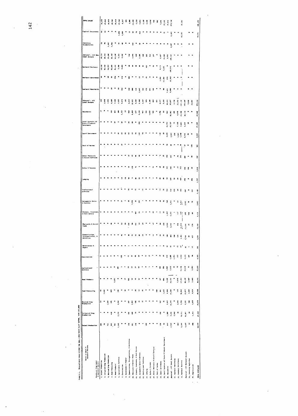
rout liut

kCflMKllllai

MoalMil t.ilM

i«a*tM«l Ctrtm^—t

KMlMtl RtM**l<«Ml

j^tatdi .jilt 5 5 5 3

i s : a : a •» ^ « -t ^ n

s n' 3 a" 3 3 5SS;3»;J;J;;5

••°J5"33

e = 5 • ' '

• »■ 3 a , -• -• -• .■"*-■ »• ;■ :■ :•

? » S 3 ?

••sir:

J I 5 i • 5 5 5 * * * 3 1

Ctftt I r**«Mii

Wlltll**

«0*d r»4ucti

r«a4 fr*c«iilB|

iMtaal PrWucllM

J = - 3 5 =

3 - 3 - S S

s:?3"32J ;

s ; * i • i i s i ? = • • » =' •' :' »' i

5 3 5 5* = *

3 S " = : S* =

• • « * s s a t } t

s. j r B ^

* s 2. s = R

» - a r r a = ^ J S I » I 3 5 « I

= = 5

! 3 • ' • ?. ?. 3 i -' •" - ; a - -

* » 3 : 3 p s -' -' a'

3 3 5 3 s •:• 3=2

: : 3 3 s c

3 « J: : ; ii i

? i i I! i i l

3 .

I i

! * i a - 1 = - I

f a I I i i i I s I I 1 i f *

1-0 ■=3-

Capital InvotMnt

Nonlocal lu*|n

Nonlocal Covcrnacnt

Nonloca I lh>u*chold»

Hou««holda

Other A|*nclaa of Stata * FaJtrat Covtriwcnt

Local Covartwant

Port of Morrow

Cafai I Tavorm

Profaitlonal SanrUai

AutOMobll* Salaa I StrvUa

Flnanca, Inturanci 1 Raat Eitaie

vholctala « Retail Trada

Coonunlcalloo, Traniportatloi I UlllllWt

o K 8 8

« o o f- Z

8 § 8 8 8 8 <=HOO — otTO 8 s

g 0 S 8 O — -O * X Q QOOOOo^r- 40000

«» o o

8S 88 8 o 8 o s

S S 8 3 Sr* -i O O «-• > O O o * a « n 'A

8 8 g 5 * » M «

8 g 8 S 8 8 » S 8 =

o o o o o S 8 8 8 0 8

s s 8

SooooO o 5 So

an * * *a i r* O » -i Q ■« ^ Oi

00Ooog5Sgsggo8gogg3:3g

Conatructlon

Hood ProJucta

Food Procaatlni

Dryland Crop Product Ion

Anl«al Product toi

o o o o o o 8 8 8 = O O Q O 8 ° 8 <u e o

o o o o o § i = 8 § a 6 = « o o o *

ooogoo|g2g = ggo|gog

S 0 8 § 0 8

o a o 1 8 3 3 3

8 = 8

O — O OMO5>*'FO>§ — ',*O -■■>o""C»»_

o o o o —/

o o o o

g = 2 8.8 8

3 8 3 8

o — — 8 8 S S 8 »* s

6 - o 8 3 S s s

5o*ooggSggoooosg-

S 9 2 8 5 8°*

a e s a s o a

a to -» So-* 8 s i

1 >

; , e e _ t 5 = ^ -•

6 ? .: I : s ~ 3 ;

a — 5 £

_ . _ o 3 2 i 2 5 4 = 3

I S I I a I o o o

5

z I •s : J ^■

3 I j ij I « i ,■ -; g

Other Agencies of State ft Federal Coverrwent

Loetl Government

Port of Morrow

00*0

« t- 1 a m — *** "*' ** K * *S o o o o o o 5 S

«o o J^ So « o

000

5 «i ? Ji 'v S t £ g

Other Wholesale loo Retail Services o o

Cofe» 5 Ttvernt

Lodjlnj


AutomoM le Sales ft Service

Finance, insurance. S Beil Estate

Mioleiale ft Retail Trnde

Communication, Transportation, S Utilities

la Intenance t Repair

Construction

Agrlculturtl Services

Kood Troducts

Food Proceislnf

Dryland Crop Production


AM nil Production

S 8 g 5 5 = S S

8 K * S

8 8 s s

o S o — 3 S S 8 S =

S 3 S S O-4 — O

— o —

8 8 — O

o 8 5 S S

; s y 8

— 1^ o en O ■* 5 —

g 5 s

8 8 8

5 i

— > v «

r E i - 4 «. 3 5

I i 1

145

APPENDIX D

INPUT-OUTPUT TABLES WITH THE

COAL FIRED POWER PLANT SECTOR

\0 : s 2 a" » a

S I i - »" s"

; ! J 8 3 5 J 3 -' -' - a i »

HMttOl ><t«ll><

ItBlilVfll l%MI*ll«IJ

3 3

a r K a • s s

= 3333 a" a" a" a a

ISSISsJa'sSa;

2 3 fl 3 ?. I 2 " ' I * a s( a ri a' *' "' ;

»«3sj«s,j,,*a»s

* • * a * s s • s | J a s a a J a • • * 5 s

3 S 3 3 3 3 I 3 5 * 5 = 3 ? ? 3 = 3 3 3 5 3 c » »3 3 a S

a- -sasiss-jississ'iaaitas;

; i s s s • »

a - 3 a a a

CiNl I Ti^.r-t

1U|B*>VII« Sll>l

C*it-Plr*d P»*

C»«mlt>ll««.

fo»J *r»<*M(*|

Mtail Praducll*!

31

a a • - a a • e 5

' 5 a * :: 3 3 5 *

3 = 3 I a

3J» = !g?.I'I

-»"B*ei« " a 3 S ?. a 3 i c 5

""*aB£3::a5»5 5

s3"j"'3°,"°"« = s

3*3°*5*2C*

3 3?. = ; :

5 5 3 * S * = 3 i J 5 " " a" s a' - -"

* s = 3 3 * 3 r j 5 3 3

a s ; i

3 3**E*;3'-E°°°5333°333S* 5

1 ! 1? ! M

11 13 i "-

11 s 1

1 f 1

I 1 i

1 1 : ]

I 3

1 c ' < r a 1 ■s : 1

nil 1 ]

Mill 3 I I i i I a a a 2 H a

I 1 ! ] I I 3 i i l I i a

1 I

a t - i I t

i a

Households

Local Agencies of State S Feder Government

Local Government

Port of Morrow

Other Wholesale 6 Retail Services

Cafes 6 Taverns

e* © ^ M \o o* t^ -* — O Tt o

r-* r~ -• «o -* u\ M -« irt rg O

r^ — rj -^ o o o o o o o —

r^ ^j -J r^ f* --

Lodging


Automobile Sales 6 Service

Finance, Insurance, 8 Real Estate

Wholesale 8 Retail Trade

Coal Fired Power Plant

Communication, Transpor- tation 6 Utilities

Maintenance 8.Repair

Construction


Wood Products

SO vO oo — O O

O o

-J -- eo

^ T-^

o^ — o —, -4

_ <o _ s s -- ^

—* r» KI —■

O —

Food Processing

DrylAnd Crop Production


Animal Production

O -4 — —' 00

' -! ' » o> >0 ^ K ►^ r-* ^

1 o r^ o\ v/1 ■* O o 3 O Ul o o (M

: o O o o "^ o o o

-. o — to —

5 i — — fl —. —J i_

148

APPENDIX E

ESTIMATION OF EMPLOYMENT MULTIPLIERS

149

Estimation Procedure

The employment multipliers for the present study were developed

in a two step process. First, employment is regressed on total sales

for firms within each endogenous sector (except households). The slope

coefficients from each sector's equation is used to develop the re-

spective sector's employment multiplier. This process was used by

Miemyk in his study of the Boulder (Colorado) economy (Miemyk,

1967). Richardson presents a discussion of this technique for esti-

mating employment multipliers in his book: Input-Output and Regional

Economics (Richardson, 1972).

Employment is regressed on total sales as follows:

Eil = ai + bi Sil i = 1, 2, ..., n - 1 (E-l)

1 = 1, 2, ..., L

where

E. = the employment by the 1th firm in the ith sector I in 1979,

S. = the total sales of the 1th firm in the ith sector II in 1979,

a. and b. = are the regression coefficients for the ith 1 1 * sector.

and

n - 1 = the number of endogenous sector (not including households), and

1 = is the number of firms sampled in the ith sector.

150

Using the (b.) coefficients, the employment multipliers are calcu-

lated for each sector, as follows:

n e. = E c.b. i = 1, 2, ... n (E-2) i i=1 iJ i

where

e. = is the employment multiplier for the ith sector,

c.. = the elements of the matrix of direct plus indirect il J coefficients, and

b. = the regression coefficient (slope) for the ith sector.

The employment multipliers (e.) portray the direct plus indirect in-

crease in employment of a sector resulting from a unit change in

sales of the respective sector.

Application

Equation (E-l) required a specific assumption with respect to

employment. As noted in Chapter III, there are two types of firms

in the sample. -- reporting and nonreporting. Employment figures

for reporting firms were obtained from the Oregon Department of

Human Services; whereas employment by nonreporting firms was not

available. It is assumed the nonreporting firms employ one FTE

(full time equivalent).—

The above assumption was tested by estimating two regressions

for each sector which contained both types of firms. The first

— Nonreporting firms with output levels such that more than one individual would be required (in the estimation of the researcher) were not used as observations in estimating the regressions.

151

equation used the data of reporting and nonreporting firms. The

second equation used only the observations of reporting firms.

In all but one case, the statistical significance of the regression

decreases when the observations for nonreporting firms were removed

from the estimation process. Thus, the observations for nonreporting

firms were used.

The results of equation (E-l) are presented in Table E-l.

Regressions were not estimated for sectors 4, 10 and 17 due to in-

sufficient observations. In turn, the (b.) coefficients -for these

three sectors were entered as zeros in equation (E-2). The regres-

sions were significant at a ninety percent level of confidence in all

but three sectors, i.e., these being Maintenance $ Repair, Cafes &

Taverns, and Local Agencies of State and Federal Government.

In Miemyk's study, the correlation coefficients for all sectors

were in excess of 0.65; and 16 out of 17 are greater than 0.50.

The results of equation (E-2) are presented in Table E-2.

The matrix of direct plus indirect coefficients from the expanded

model (incorporates the CFPP sector) was used to calculate the em-

ployment multipliers.

TABLE E-1. RESULTS OF REGRESSING EMPLOYMENT ON TOTAL SALES, BY SECTOR

Sector Coefficient Number of Call culated Coefficient

(Slope) r2 Observations F ' Value (Constant)

.0000128 .56 13 14.2 .67

.0000582 .99 6 2 ,754.2 -.58

.0000064 .25 27 8.44 1.15 NA* NA 2 NA NA

.0000114 .99 4 39 ,442.9 .23

.0000012 .89 10 67.6 3.10

.0000136 .89 11 73.1 .08

.0000396 .45 3 .1 -.19

.0000132 .93 4 25.0 4.48 NA NA NA NA NA

.0000100 .41 14 8.4 1.96

.0000239 .82 6 18.0 -.17

.0000128 .86 11 56.9 -.10

.0000739 .40 8 4.0 -2.58

.0000543 .88 5 21.3 -1.43

.0000454 .36 7 2.8 4.18

.0000625 .83 8 29.5 .36 NA NA 1 NA NA

.0000257 .99 7 2 ,140.9 2.72

.0000008 .09 8 .6 2.51

1. Animal Production 2. Irrigated Crop Production 3. Dryland Crop Production 4. Food Processing 5. Wood Products 6. Agricultural Services 7. Construction 8. Maintenance § Repair 9. Communication, Transportation 5

Utilities 10. Coal Fired Power Plant 11. Wholesale § Retail Trade 12. Finance, Insurance § Real Estate 13. Automobile Sales § Service 14. Professional Services 15. Lodging 16. Cafes £ Taverns 17. Other Wholesale § Retail

Services 18. Port of Morrow 19. Local Government 20. Local Agencies of State §

Federal Government

N.A. indicates that insufficient data was available to estimate the coefficient. on

153

TABLE E-2. EMPLOYMENT MULTIPLIERS FOR THE MORROW COUNTY INPUT- OUTPUT MODEL, BY SECTOR

Sector Multiplier




4. Food Processing

5. Wood Products


7. Construction


9. Communication, Transportation § Utilities


11. Wholesale 5 Retail Trade

12. Finance, Insurance, § Real Estate

13. Automobile Sales 5 Service


15. Lodging

16. Cafes 5 Taverns

17. Other Wholesale & Retail Services

18. Port of Morrow



.0000213

.0000695

.0000127

N.A. *

.0000166

.0000015

.0000179

.0000655

.0000186

N.A.

.0000129

.0000487

.0000188

.0001298

.0000835

.0000744

.0001251

N.A.

.0000516

.0000017

N.A. indicates that insufficient data was available to estimate the multiplier.

154

APPENDIX F

MATRIX OF DIRECT PLUS INDIRECT COEFFICIENTS

SIMULATING THE COAL FIRED POWER PLANT

WITH ENDOGENOUS SALES

in

5 a

Households

Local Agencies of State fl Federal Government

Local Government

Port of Morrow

Other Wholesale 6 Retail Services

Cafes 6 Taverns

Lodging


Automobile Sales 8 Service

Finance, Insurance, G Real Estate

Wholesale 8 Retail Trade

Coal-Fired Power Plant

Comiminlcatlon; Transports tlon 8 Utilities

Maintenance 8 Repair

Construction


Wood Products

-J f~ Kl —t ya _.

o o a o

o — —

*o t^- -*

o -< ^

(W -*

M —.

Food Processing

Dryland Crop Production


Animal Production

Presented on July 29, 1981 Title: MODIFICATIONS OF STATIC ...

Documents

Transcript of Presented on July 29, 1981 Title: MODIFICATIONS OF STATIC ...