Sample size estimation

Presented by :Dr. Reshma.S Moderator : Dr. Subodh S Gupta

Why do we need sample size calculation?

When should we calculate sample size?

Basic principles for sample size calculation

Derivation of sample size formula

Description of some commonly used terms

Practical issues in calculating sample size

Procedure for calculating sample size

Formulae for calculation of sample size in different study design

Framework

Sample Size (n) is the number of individuals in a group under study

If the sample size is too small, even the most rigorously executed study may fail to answer its research question, may fail to detect important effects or associations, or may estimate those effects or associations too imprecisely

If the sample size is too large, the study will be more difficult and costly,

and may even lead to a loss in accuracy, as it is often difficult to maintain

high data quality.

Hence, it is necessary to estimate the optimum sample size for each

individual study

Why do we need sample size calculation?

Sample size can be addressed at two stages of the actual conduct of the study

Firstly, calculate the optimum sample size required during the planning stage, while designing the study, using appropriate approaches and some information on parameters.

Secondly, sample size can also be calculated in between the study. For example in rare case study sample size can be re evaluated after mid-term evaluation

When should we calculate sample size?

Sample size primarily depend on:• Availability of resource• Proposed plan of analysis

Sample size estimation requires:• Estimate of the variable of interest (e.g. mean, proportion, OR, RR)• Desired precision

Select the confidence level for the interval (e.g. 95% or 99%) and power of the study

State the null hypothesis and alternative hypothesis.

Loss to follow up

Basic principles for sample size calculation

Standard error, SE = n = --------------------------(1) if ‘d’ is the unit on either side of point estimate, then, d = Z (1-α)*SE of mean Then , SE = Now, putting the value of SE in (1), we have n =

Derivation of sample size formula:

Random error Systematic error (bias) Precision (Reliability) Null hypothesis Alternative hypothesis Type I error (α) Type II error (β) Hypothesis Testing Power of the study (1-β) Design effect

Description of some commonly used terms:

It describes the role of chance Sources of random error include:• sampling variability • subject to subject differences• measurement errors

It can be controlled and reduced to acceptably low levels by:

• Increasing the sample size• Repeating the experiment

Random error

It describes deviations that are not a consequence of chance alone Several factors including patient selection criteria might contribute to

it. These factors may not be amenable to measurement Removed or reduced by good design and conduct of the experiment A strong bias can yield an estimate very far from the true value

Systematic error (bias)

Degree to which a variable has the same value when measured several times

It is a measure of consistency

It is a function of :• random error (the greater the error, the less precise the measurement)• sample size• confidence interval required &

A larger sample size would give precise estimates

Precision (Reliability)

It indicates the degree to which the variable actually represents

what it is supposed to represent

It is a function of systematic error

The greater the error the less accurate the variable

Accuracy (Validity)

Null hypothesis is a hypothesis which states that there is no difference among groups or that there is no association between the predictor and the outcome variables

This hypothesis needs to be tested

Null hypothesis

It assumes that there is a difference among the groups or there exists an association between the predictor and outcome variable

There are two types of alternative hypothesis:• one-tailed (one-sided) hypothesis &• two-tailed (two-sided) hypothesis

One-tailed hypothesis specifies the difference (or effect or association) in one direction only.

Two-tailed hypothesis specifies the difference (or effect or association) in either direction.

Alternative hypothesis

Truth In the population

Hₒ (False) Hₒ(True)

Results in the study

Reject hypothesis

Correct Type I error

Accept hypothesis

Type II error correct

Hypothesis testing

Type I error Type II error

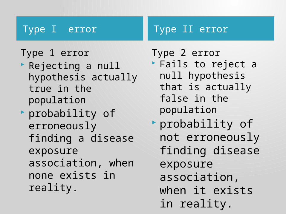
Type 1 error Rejecting a null hypothesis

actually true in the population

probability of erroneously finding a disease exposure association, when none exists in reality.

Type 2 error Fails to reject a null

hypothesis that is actually false in the population

probability of not erroneously finding disease exposure association, when it exists in reality.

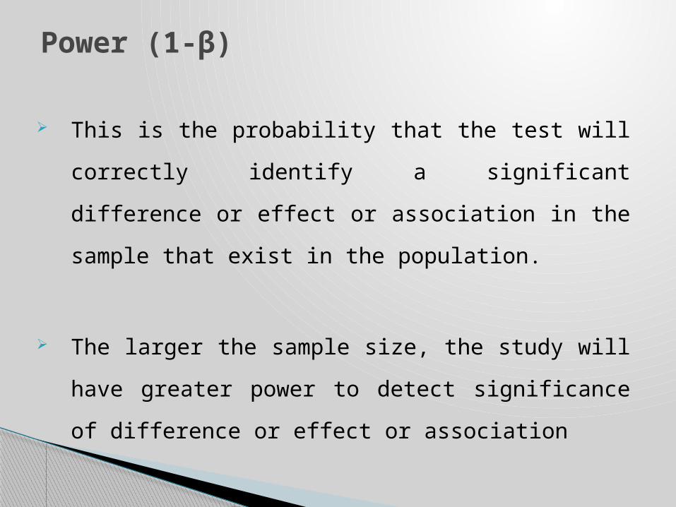
This is the probability that the test will correctly identify a

significant difference or effect or association in the sample

that exist in the population.

The larger the sample size, the study will have greater power

to detect significance of difference or effect or association

Power (1-β)

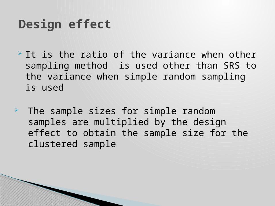
It is the ratio of the variance when other sampling method is used other than SRS to the variance when simple random sampling is used

The sample sizes for simple random samples are multiplied by the design effect to obtain the sample size for the clustered sample

Design effect

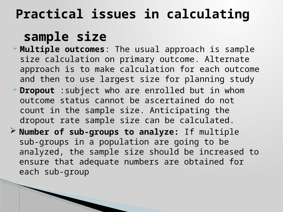
Multiple outcomes: The usual approach is sample size calculation on primary outcome. Alternate approach is to make calculation for each outcome and then to use largest size for planning study

Dropout :subject who are enrolled but in whom outcome status cannot be ascertained do not count in the sample size. Anticipating the dropout rate sample size can be calculated.

Number of sub-groups to analyze: If multiple sub-groups in a population are going to be analyzed, the sample size should be increased to ensure that adequate numbers are obtained for each sub-group

Practical issues in calculating sample size

Use of formula

Readymade tables

Nomograms

Computer software

Procedure for calculating sample size:

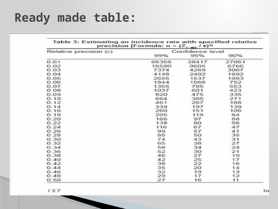
Ready made table:

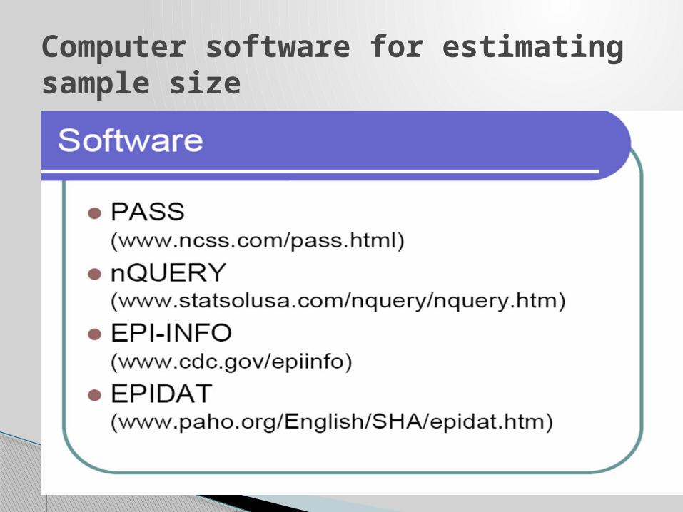
Computer software for estimating sample size

Cross sectional study

Case control study

Cohort study

Clinical trial

Formulae for calculation of sample size in

different study design :

Cross sectional study

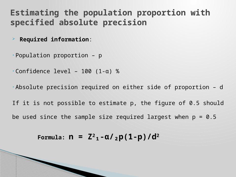
Required information:

• Population proportion – p

• Confidence level – 100 (1-α) %

• Absolute precision required on either side of proportion – d

If it is not possible to estimate p, the figure of 0.5 should be used since

the sample size required largest when p = 0.5

Formula: n = Z2₁-α/₂p(1-p)/d2

Estimating the population proportion with specified absolute precision

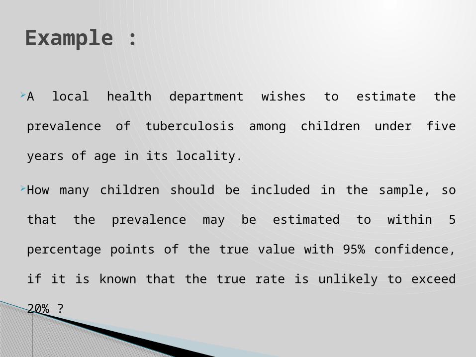
A local health department wishes to estimate the prevalence of

tuberculosis among children under five years of age in its locality.

How many children should be included in the sample, so that the

prevalence may be estimated to within 5 percentage points of the

true value with 95% confidence, if it is known that the true rate is

unlikely to exceed 20% ?

Example :

Anticipated population proportion =20 % (p=0.20)

Confidence level = 95%

Absolute precision (15 %-25 %) = 5 percentage points (d=0.05)

By using the above formula, we have

n = 1.962 x 0.2 x (1 - 0.2) / (0.05)2

= 245.86

i.e. 246

Solution :

Required information:

Anticipated population proportion = P

Confidence level = 100(1-α)%

Relative precision = ε

Formula:

n = Z21-α/2 (1-p)/ ε 2P

Estimating a population proportion with specified relative precisions

An investigator working for the national program of

immunization seeks to estimate the proportion of children in

country who are receiving appropriate childhood vaccinations.

How many children must be studied if the resulting estimate is

to fall within 10% of true proportion with 95% confidence?

The vaccination coverage is not expected to be below 50%.

Example:

Anticipated population proportion = 50%

Confidence level = 95%

Relative precision (45%-55%) =10% of 50% (ε =0.10)

n = Z21-α/2 (1-P)/ ε 2P

= 1.962 x (1- 0.5) /0.102 x 0.5

= 384.16

Solution :

Required information:

test value of population proportion under the null hypothesis = Po

Anticipated value of the population proportion = Pa

Level of significance = 100 α %

Power of the test = 100 (1-β)%

Alternative hypothesis Pa>Po or Pa<Po for one sided

Pa ≠ Po for two sided

Formula: n= {Z1-α √[Po(1-Po)+ Z1-β√[Pa(1-Pa)]}²/ (Po-Pa)2

Hypothesis test for population proportion

Previous surveys have demonstrated that the usual prevalence of

dental caries among school children in a particular community is

about 25%.

How many children should be included in a survey designed to

test for a decrease in the prevalence of dental caries, if it is desired

to be 90% sure of detecting a rate of 20% at the 5% level of

significance?

Example :

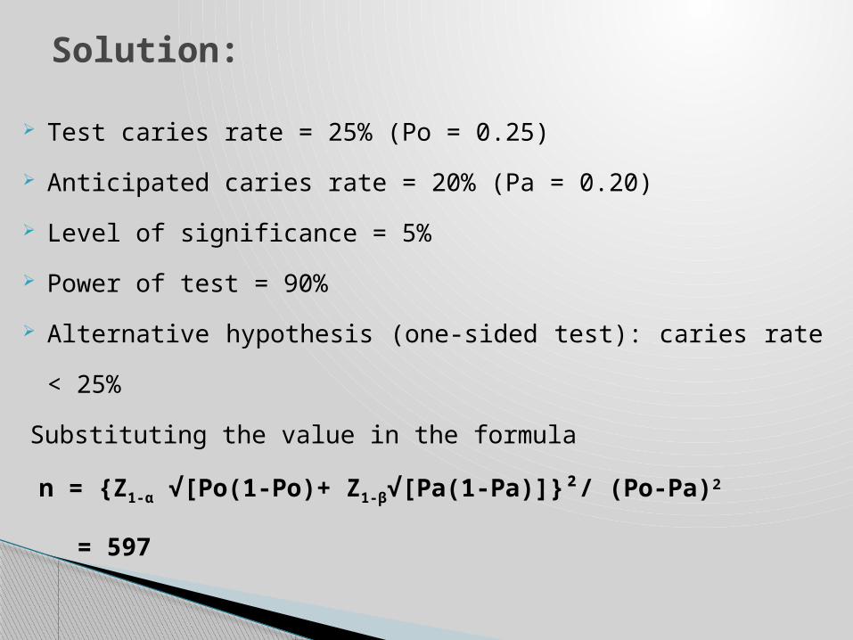
Test caries rate = 25% (Po = 0.25)

Anticipated caries rate = 20% (Pa = 0.20)

Level of significance = 5%

Power of test = 90%

Alternative hypothesis (one-sided test): caries rate < 25%

Substituting the value in the formula  

n = {Z1-α √[Po(1-Po)+ Z1-β√[Pa(1-Pa)]}²/ (Po-Pa)2

= 597

Solution:

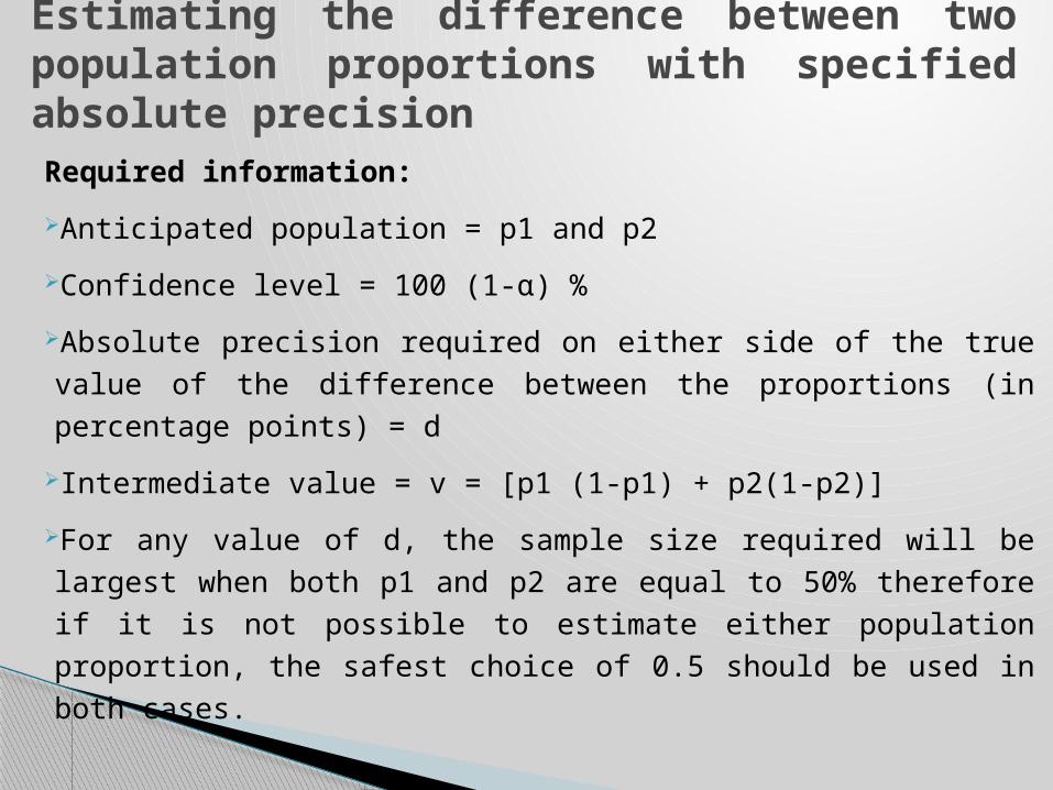
Required information:

Anticipated population = p1 and p2

Confidence level = 100 (1-α) %

Absolute precision required on either side of the true value of the difference

between the proportions (in percentage points) = d

Intermediate value = v = [p1 (1-p1) + p2(1-p2)]

For any value of d, the sample size required will be largest when both p1 and p2

are equal to 50% therefore if it is not possible to estimate either population

proportion, the safest choice of 0.5 should be used in both cases.

Formula: n= Z²₁-α[p1(1-p1)+p2(1-p2)]²/d²

Estimating the difference between two population proportions with specified absolute precision

What sample size should be selected from each of two

groups of people to estimate a risk difference to within 5

percentage points of the true difference with 95%

confidence, when no reasonable estimate of p1 and p2 can

be made?

Example:

Anticipated population proportion, p1=50%, p2=50%

Confidence level = 95 %

Absolute precision = 5 %

Intermediate value = 0.50 {v=[p1 (1-p1) + p2(1-p2)]}

By using the formula n = Z²₁-α[p1(1-p1)+p2(1-p2)]²/d²

we get n = 768

Solution:

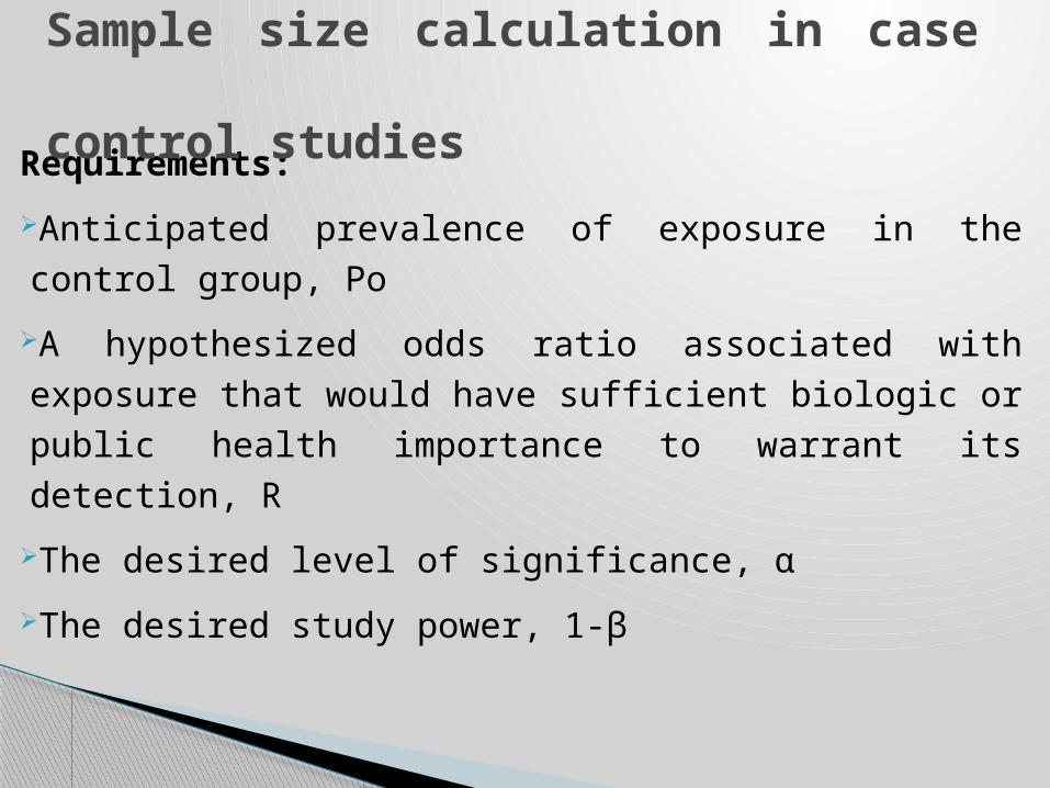
Requirements:

Anticipated prevalence of exposure in the control group, Po

A hypothesized odds ratio associated with exposure that would have

sufficient biologic or public health importance to warrant its detection,

R

The desired level of significance, α

The desired study power, 1-β

Sample size calculation in case control studies

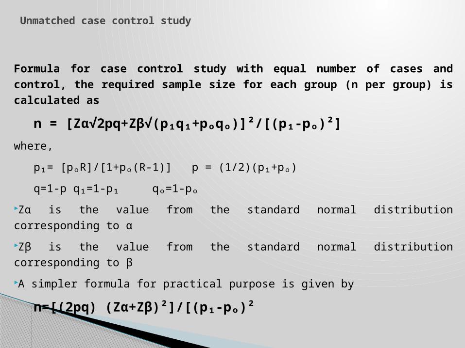
Formula for case control study with equal number of cases and control, the

required sample size for each group (n per group) is calculated as

n = [Zα√2pq+Zβ√(p₁q₁+pₒqₒ)]²/[(p₁-pₒ)²]

where,

p₁= [pₒR]/[1+pₒ(R-1)] p = (1/2)(p₁+pₒ)

q=1-p q₁=1-p₁ qₒ=1-pₒ

Zα is the value from the standard normal distribution corresponding to α

Zβ is the value from the standard normal distribution corresponding to β

A simpler formula for practical purpose is given by

n=[(2pq) (Zα+Zβ)²]/[(p₁-pₒ)²

Unmatched case control study

Case control study:

Congenital heart defects

Women using oral contraceptives occurring around the time of

conception.

 30% of women of child bearing age will have an exposure to

within 3 months of conception

Example :

Congenital heart defects Women using oral contraceptives occurring around the time of

conception  30% of women of child bearing age will have an exposure to within 3

months of conception

Here, pₒ = 0.30 α = 0.05(two sided) Zα=1.96 β= 0.10 Zβ=1.28 R = 3

Now p₁= [0.3x3] / [1+0.3(3-1)] = 0.5625 P = (1/2) (0.3+0.5625) = 0.43125

n = [1.96√(0.4905) + 1.28√(0.2461+0.21)] / [(0.2625)²]

= 73

EXAMPLE:

n= [Zα√(1+1/c)pq + Zβ√(p₁q₁+pₒqₒ/c)]²/[(p₁-pₒ)²]

where,

p = (p₁+cpₒ)/ (1+c)

p₁= [pₒR]/ [1+pₒ(R-1)]

 

Equivalent simpler formula is

n= [(1+1/c)pq) (Zα+Zβ)²]/[(p₁-pₒ)²]

Sample size formula in a case control studywith ‘c’ control per case is given by:

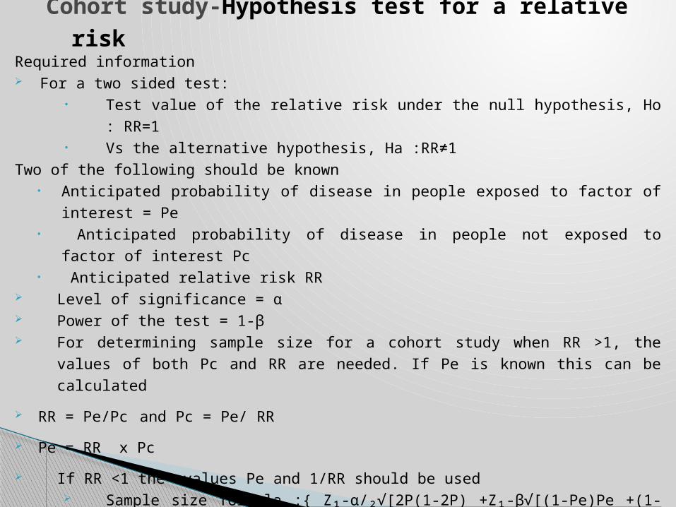
Required information For a two sided test:

• Test value of the relative risk under the null hypothesis, Ho : RR=1• Vs the alternative hypothesis, Ha :RR≠1

Two of the following should be known• Anticipated probability of disease in people exposed to factor of interest = Pe• Anticipated probability of disease in people not exposed to factor of interest Pc• Anticipated relative risk RR

Level of significance = α Power of the test = 1-β For determining sample size for a cohort study when RR >1, the values of both Pc and RR are

needed. If Pe is known this can be calculated

RR = Pe/Pc and Pc = Pe/ RR

Pe = RR x Pc

If RR <1 the values Pe and 1/RR should be used Sample size formula :{ Z₁-α/₂√[2P(1-2P) +Z₁-β√[(1-Pe)Pe +(1-Pc)Pc]}² (Pe-Pc)²

Where p=(Pe+Pc)/2

Cohort study-Hypothesis test for a relative risk

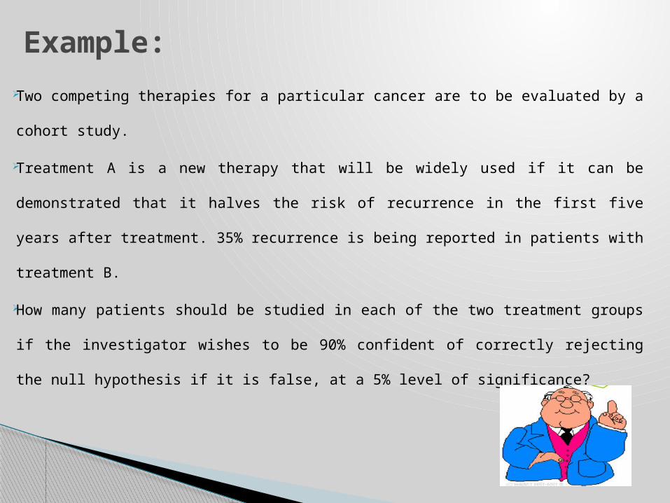
Two competing therapies for a particular cancer are to be evaluated by a cohort

study.

Treatment A is a new therapy that will be widely used if it can be demonstrated

that it halves the risk of recurrence in the first five years after treatment. 35%

recurrence is being reported in patients with treatment B.

How many patients should be studied in each of the two treatment groups if the

investigator wishes to be 90% confident of correctly rejecting the null hypothesis

if it is false, at a 5% level of significance?

Example:

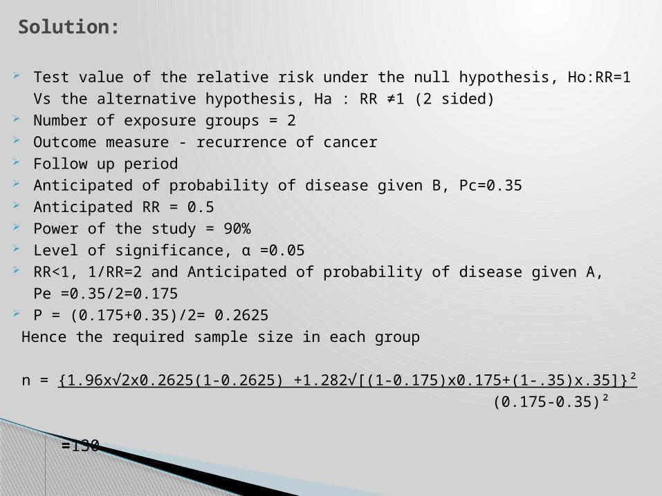
Test value of the relative risk under the null hypothesis, Ho:RR=1

Vs the alternative hypothesis, Ha : RR ≠1 (2 sided) Number of exposure groups = 2 Outcome measure - recurrence of cancer Follow up period Anticipated of probability of disease given B, Pc=0.35 Anticipated RR = 0.5 Power of the study = 90% Level of significance, α =0.05 RR<1, 1/RR=2 and Anticipated of probability of disease given A,

Pe =0.35/2=0.175 P = (0.175+0.35)/2= 0.2625

 Hence the required sample size in each group

 

n = {1.96x√2x0.2625(1-0.2625) +1.282√[(1-0.175)x0.175+(1-.35)x.35]}²

(0.175-0.35)²

=130

Solution:

Required information

The following should be known

• relative precision, ε

• confidence level, (1-α)

• Sample size formula

n= [Z/ ε]²

where Z value corresponds to appropriate level of significance

Estimating an incidence rate with a specified relative precision

How large a sample of patients should be followed up if an investigator

wishes to estimate the incidence rate of a disease to within 10% of its true

value with 95% confidence?

Solution

Relative precision, ε = 0.01

Confidence level, (1-α) = 0.95

Required sample size is

n = [1.96/.10]²

=384

Example:

Required information

Test value of the incidence rate under the null hypothesis, Ho:λ=λₒ

• Vs the alternative hypothesis, Ha :λ≠λₒ (or λ=λa)

• Or Ho:λₒ =λa Vs Ha :λₒ ≠λa

Anticipated value of the population incidence rate = λa

Power of test 1-β

Level of significance α

Sample size formula

n = ( Z₁-α/₂ λₒ+Z₁-β λa )²

(λₒ-λa)²

Hypothesis test for an incidence rate

On the basis of a five year follow up study of a small number

of people, the annual incidence rate of a particular disease is

reported to be 40%.

What minimum sample size would be needed to test the

hypothesis that the population incidence rate is different from

40% at the 5% level of significance?

It is desired that the test should have a power of 90% of

detecting a true annual incidence rate of 50%.

Example:

Test value of the population incidence rate under the null hypothesis,

Ho:λₒ=.40

Anticipated value of the population incidence rate (under Ha), λa=0.50

Power of test 1-β = 0.90

Level of significance, α = 0.05

• Required sample size is

n = (1.96x .40+ 1.282x.50)²

(0.40-0.50)²

= 203

Solution:

Design specifications affecting sample considerations in clinical trials

Number of treatment groups

Outcome measures

Length of follow-up

Alternative hypothesis

Treatment difference

Type I and Type II error protection

Allocation ratio

Sample size estimation for Clinical trial

Rate of loss to follow up

Noncompliance rate

Treatment lag time

Degree of stratification for baseline risk factors

α and β levels adjustment for multiple comparisons

α and β levels adjustment for multiple looks

α and β levels adjustment for multiple outcomes

Design specifications affecting sample considerations in clinical

trials Cont.

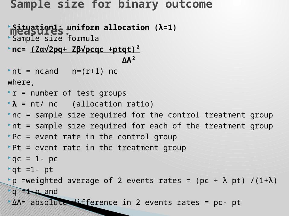
Situation1: uniform allocation (λ=1) Sample size formula nc= (Zα√2pq+ Zβ√pcqc +ptqt)²

ΔA² nt = nc and n=(r+1) nc

where, r = number of test groups λ = nt/ nc (allocation ratio) nc = sample size required for the control treatment group nt = sample size required for each of the treatment group Pc = event rate in the control group Pt = event rate in the treatment group qc = 1- pc qt =1- pt p =weighted average of 2 events rates = (pc + λ pt) /(1+λ) q =1-p and ΔA= absolute difference in 2 events rates = pc- pt

Sample size for binary outcome measures:

Design specification:

• number of treatment group= 2

• outcome measure: 5 year mortality

• alternative hypothesis: one sided

• detectable treatment difference : 10% difference in 5 year mortality of two group

• pc=0.40

• pt== 0.30

• error protection: α(one sided)=0.05, β=0.05

• allocation ratio: 1:1, λ=1

• loss due to drop out and non compliance:d=20%

Example : (cardiovascular mortality study)

nc = 1.645√2(0.35)(0.65) + 1.645√(0.4x0.6 +0.3x0.7)²

(0.10)²

= 490

Adjusting for 20% losses,

nc = 490 x (1/.8)

= 613

nt = 613

Total sample size n = 613+613

=1226

Solution:

Sample size formula

nc = (Zα√(λ+1)/λ + Zβ√(pcqc +ptqt/λ)²

ΔA²

nt= λ nc

and n = r nt + nc

non uniform allocation (λ≠1)

Design specification: number of treatment group= 6 (1 control and 5 test treatments) outcome measure: 5 year mortality alternative hypothesis: one sided detectable treatment difference : 25% difference in 5 year

mortality of test group in relation to control group pc=0.30, ΔA== pc- pt/ pc= 0.25 i.e.pt== 0.225 error protection: α(one sided)=0.01, β=0.05 allocation ratio: 1:1:1:1:2.5, λ=1/2.5 loss due to drop out and non-compliance: d=30% after 5 year

follow up

Example: coronary drug project

Sample size calculation

nc=

(2.326√0.28x0.72(0.4+1+1.645√(0.3x0.7+0.225x0.775/0.4)²

(0.075)²

=1906

nt=1906x (1/2.50 )= 762

Adjusting for 30% losses,

nc= 1906x(1/1-0.3)=2723

nt= 763x(1/.7)= 1089

Total sample size= 5(1089) +2723= 8168

The sample size in a diagnostic test study is done in two stages

First, specify the expected “sensitivity” of the test and specify the “acceptable deviation” from this

sensitivity on either side of the expected sensitivity. Then,

a = sensitivity (1-sensitivity)

(deviation)²

Let us say, we are validating ELISA test for HIV infection. Our rough estimate is that the sensitivity

would be 95% (i.e. 0.95) and we accept a deviation of 3% on either side

(i.e. acceptable range of sensitivity to be detected by the present study sample = 92% to 98%); thus d =

3% (i.e.0.03).

a= 0.95(1-0.95)

(0.03)²

= 53

Calculation of sample size in diagnostic test:

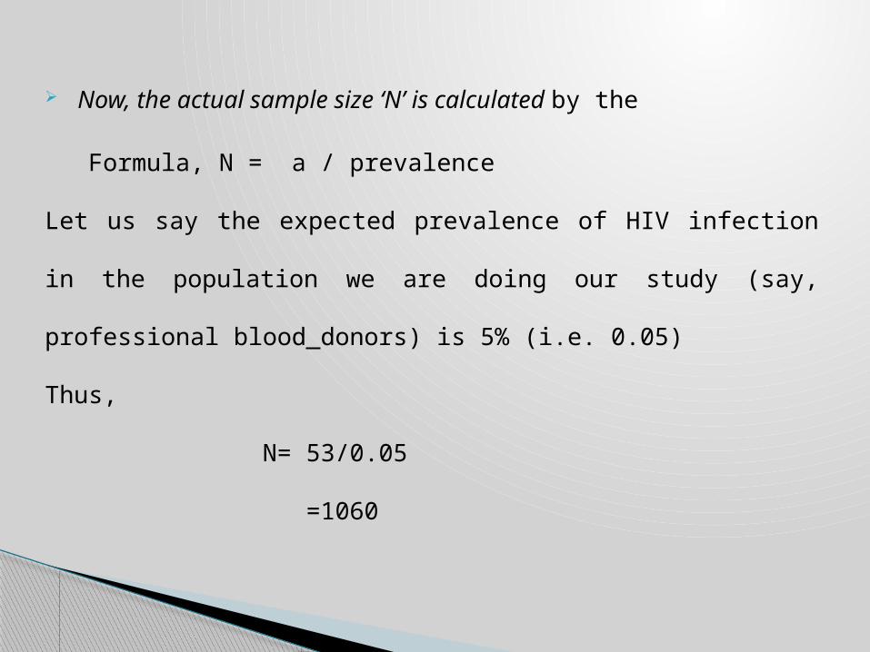
Now, the actual sample size ‘N’ is calculated by the

Formula, N = a / prevalence

Let us say the expected prevalence of HIV infection in the population we are

doing our study (say, professional blood donors) is 5% (i.e. 0.05)

Thus,

N= 53/0.05

=1060

1. Lwanga SK, Lemeshow S. Sample size determination in health studies - A practical

manual. 1st ed. Geneva: World Health Organization; 1991.  

2. Zodpey SP, Ughade SN. Workshop manual: Workshop on Sample Size Considerations

in Medical Research. Nagpur: MCIAPSM; 1999

3. Zodpey SP. Sample size and power analysis in medical research. Indian J Dermatol

Venerol Leprol 2004;70(2):123-28

4. Rao Vishweswara K. Biostatistics A manual of statistical methods for use in health ,

nutrition and anthropology. 2nd edition. New Delhi: Jaypee brothers;2007

5. Bhalwar R et al. Text book of Public Health and Community Medicine 1st ed.

Pune :Department of Community Medicine Armed Forces Medical College; 2009

References :