Presented at the 2011 ISPA/SCEA Joint Annual Conference ... · An Improved Method for Predicting...

1

An Improved Method for Predicting Software Code Growth:

Tecolote DSLOC Estimate Growth Model Michael A. Ross Technical Expert

Tecolote Research, Inc. 3601 Aviation Blvd., Suite 1600

Manhattan Beach, CA 90266-3756 310-536-0011

[email protected] http://www.tecolote.com

1,2Abstract— This paper describes a model and methodology developed for Tecolote Research, Inc. by this paper’s author and referred to as the Tecolote DSLOC Estimate Growth Model v06. The model provides probabilistic growth adjustment to single-point Technical Baseline Esti-mates (TBEs) of Delivered Source Lines of Code (DSLOC), for both New software and Pre-Existing Reused (PER) software, that is sensitive to the maturity of the estimate; i.e., when, in the Software Development Life Cycle (SDLC), the DSLOC TBE is performed. The model is based on Software Resources Data Report (SRDR) data collected by Dr. Wilson Rosa of the U.S. Air Force Cost Analysis Agency (AFCAA). This model provides an alternative to other software code growth methodologies such as Mr. Barry Holchin’s (2003) code growth matrix.

TABLE OF CONTENTS

1. INTRODUCTION .........................................................................................................................1 2. MODEL SUMMARY ...................................................................................................................2 3. COMPONENTS OF THE MODEL .................................................................................................3 4. MODELING DSLOC GROWTH IN TECOLOTE’S ACEIT TOOL ............................................10 5. MODELING DSLOC GROWTH IN GALORATH’S SEER-SEM TOOL ....................................11 6. CONCLUSION ..........................................................................................................................18 REFERENCES ..................................................................................................................................19 BIOGRAPHY ...................................................................................................................................20

1. INTRODUCTION

The Tecolote DSLOC Estimate Growth Model v06, developed for Tecolote Research, Inc. by the author of this paper, provides probabilistic growth adjustment to single-point Technical Baseline Estimates (TBEs) of Delivered Source Lines of Code (DSLOC), for both New software and Pre-Existing Reused (PER) software, that are sensitive to the maturity of the estimate; i.e., when, in

1 © Tecolote Research, Inc. All rights reserved. 2 1st Edition, Version 05; April 18, 2011

Presented at the 2011 ISPA/SCEA Joint Annual Conference and Training Workshop - www.iceaaonline.com

2

the Software Development Life Cycle (SDLC), the DSLOC TBE is performed. It is a data driven model and methodology that is based on Software Resources Data Report (SRDR) data collected by Dr. Wilson Rosa of the U.S. Air Force Cost Analysis Agency (AFCAA). This model provides an alternative to other software code growth methodologies such as Mr. Barry Holchin’s (2003) code growth matrix.

The paper includes custom Cumulative Distribution Function (CDF) tables that can be copied into tools such as Tecolote’s ACEIT or Oracle’s Crystal Ball in order to create the Custom CDFs that are needed to model the baseline New DSLOC growth factor distribution and to model the baseline Pre-Existing Reused DSLOC growth factor distribution. The paper also includes a set of DSLOC growth factor multipliers as a function of Estimate Maturity for each of New DSLOC and Pre-Existing DSLOC such that appropriate application of these factors to a DSLOC TBE yields corresponding Least, Likely, and Most DSLOC values that, if input to Galorath’s SEER-SEM, will reasonably model growth and uncertainty consistent with the SRDR historical data.

2. MODEL SUMMARY

The Tecolote DSLOC Estimate Growth Model v06 equations for applying growth and uncertain-ty to TBE New and PER DSLOC are3

1 1btD_NewS e D_Adj_New GF_NewS K (1)

and

1 1btD_PERS e D_Adj_PER GF_PERS K (2)

where

growth-adjusted New DSLOC estimate distribution

growth-adjusted PER DSLOC estimate distribution

Technical Baseline Estimate (TBE) of New DSLOC

Technical Baseline E

D_New

D_PER

S

S

D_Adj_New

D_Adj_PER

S

S

stimate (TBE) of PER DSLOC

baseline (Estimate Maturity 0 ) New DSLOC growth factor distribution

(provided custom CDF in Table 3)

baseline (Estimate Maturity 0 ) PER DSLOC growth factor di

%

%

GF_New

GF_PER

K

K stribution

(provided custom CDF in Table 3)

decay constant; default is 3 466 based on Boehm's "Cone of Uncertainty"

(Boehm, 1981, p. 311)

Estimate Maturity Parameter: (SDLCBegin 0 ; SyRR 20 ; SwRR 4

.

% %

b

t

0 ;

SwPDR 60 ; SwCDR 80 ; SwAccept 100 )

%

% % %

3 We use the Arial bold italic font to denote random variables; i.e., variables that can take on values according to some probability distribution.


3

The equations for providing the appropriate New and PER , ,Least Likely Most DSLOC inputs

to Galorath’s SEER-SEM tool are

3 466 3 466

3 466

Growth-Adjusted New DSLOC Growth-Adjusted PER DSLOC

0 828071 1 0 687191 1

0 828071 1 0

. .

.

. .

.

t tD_Adj_New_Least D_New D_Adj_PER_Least D_PER

tD_Adj_New_Likely D_New D_Adj_PER_Likely D_PER

S S e S S e

S S e S S

3 466

3 466 3 466

687192 1

5 366128 1 3 658219 1

.

. .

.

. .

t

t tD_Adj_New_Most D_New D_Adj_PER_Most D_PER

e

S S e S S e

(3)

The remainder of this paper describes the basis of these equations.

3. COMPONENTS OF THE MODEL

Normalized Estimate Maturity

The single parameter input to the Tecolote DSLOC Estimate Growth Model is normalized Esti-mate Maturity t . By default, Estimate Maturity is quantified by the scale contained in Table 1 below. This scale is consistent with the model defaults for the baseline New and Pre-Existing DSLOC growth factor distributions (which is based on the SRDR data) and with the uncertainty decay factor (which is based on Boehm’s (1981) Cone of Uncertainty. Tailored instances of the model can be created for different SDLCs as long as historical data exists where the projects followed that particular SDLC and where this data has been used to determine corresponding baseline growth factor distributions and uncertainty decay factor values or distributions.

Table 1 Default Normalized Estimate Maturity Scale

DSLOC Baseline Growth Factor Distributions

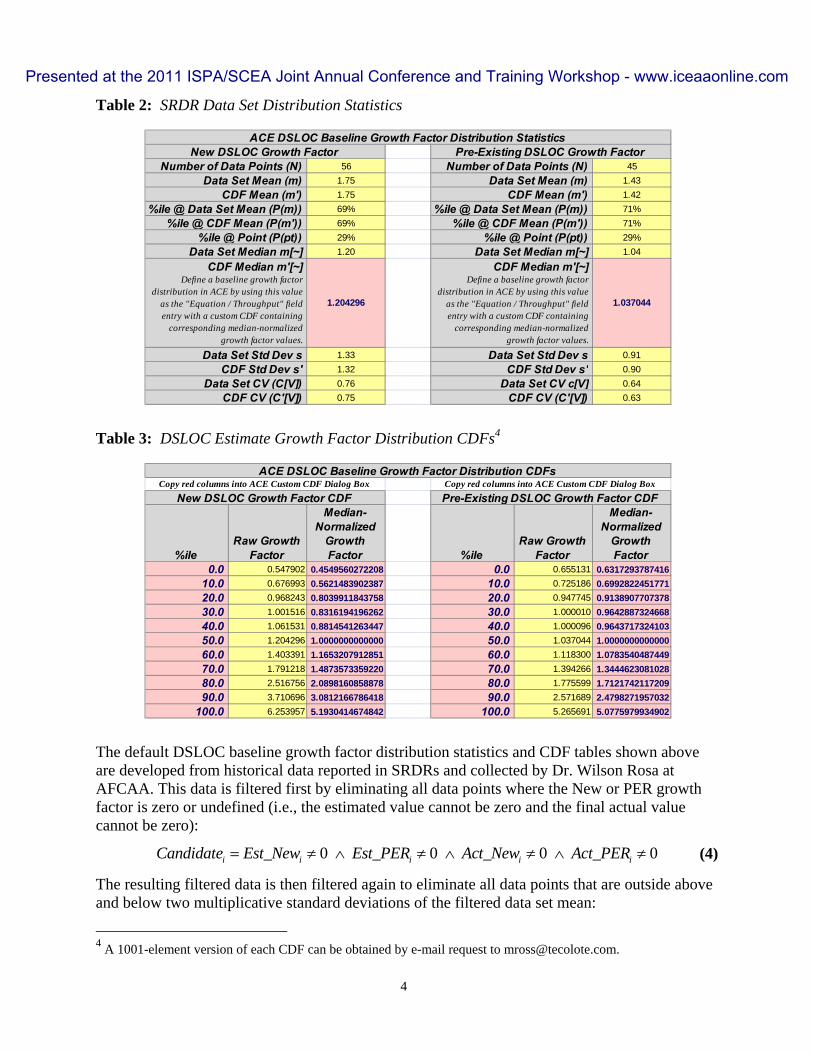
DSLOC estimate growth is modeled at the computer program (CSCI) level and is applied by multiplying the TBEs of New and Pre-Existing DSLOC by the appropriate decay-adjusted growth factor distribution. The baseline (zero Estimate Maturity) growth factor distributions for New DSLOC and for Pre-Existing DSLOC have the following characteristics (Table 2) and cus-tom CDFs (Table 3).

Estimate Maturity Scalet = 0%

t = 20%

t = 40%

t = 60%

t = 80%

t = 100%

Software Preliminary Design ReviewSoftware Critical Design ReviewSoftware Acceptance

Begin SDLCSystem Requirements ReviewSystem Design Review / Software Requirements Review


4

Table 2: SRDR Data Set Distribution Statistics

Table 3: DSLOC Estimate Growth Factor Distribution CDFs4

The default DSLOC baseline growth factor distribution statistics and CDF tables shown above are developed from historical data reported in SRDRs and collected by Dr. Wilson Rosa at AFCAA. This data is filtered first by eliminating all data points where the New or PER growth factor is zero or undefined (i.e., the estimated value cannot be zero and the final actual value cannot be zero):

0 0 0 0i i i i iCandidate Est_New Est_PER Act_New Act_PER (4)

The resulting filtered data is then filtered again to eliminate all data points that are outside above and below two multiplicative standard deviations of the filtered data set mean:

4 A 1001-element version of each CDF can be obtained by e-mail request to [email protected].

56 45

1.75 1.43

1.75 1.42

69% 71%

69% 71%

29% 29%

1.20 1.04

1.204296 1.037044

1.33 0.91

1.32 0.90

0.76 0.64

0.75 0.63CDF CV (C′[V]) CDF CV (C′[V])

CDF Mean (m′) CDF Mean (m′)

%ile @ CDF Mean (P(m′)) %ile @ CDF Mean (P(m′))

CDF Median m′[~]Define a baseline growth factor

distribution in ACE by using this value as the "Equation / Throughput" field entry with a custom CDF containing

corresponding median-normalized growth factor values.

CDF Median m′[~]Define a baseline growth factor

distribution in ACE by using this value as the "Equation / Throughput" field entry with a custom CDF containing

corresponding median-normalized growth factor values.

Data Set Median m[~] Data Set Median m[~]

Data Set Std Dev s Data Set Std Dev s

Data Set CV (C[V]) Data Set CV c[V]

%ile @ Data Set Mean (P(m)) %ile @ Data Set Mean (P(m))

%ile @ Point (P(pt)) %ile @ Point (P(pt))

CDF Std Dev s′ CDF Std Dev s′

Data Set Mean (m) Data Set Mean (m)

ACE DSLOC Baseline Growth Factor Distribution StatisticsNew DSLOC Growth Factor Pre-Existing DSLOC Growth Factor

Number of Data Points (N) Number of Data Points (N)

%ileRaw Growth

Factor

Median-Normalized

Growth Factor %ile

Raw Growth Factor

Median-Normalized

Growth Factor

0.0 0.547902 0.4549560272208 0.0 0.655131 0.6317293787416

10.0 0.676993 0.5621483902387 10.0 0.725186 0.6992822451771

20.0 0.968243 0.8039911843758 20.0 0.947745 0.9138907707378

30.0 1.001516 0.8316194196262 30.0 1.000010 0.9642887324668

40.0 1.061531 0.8814541263447 40.0 1.000096 0.9643717324103

50.0 1.204296 1.0000000000000 50.0 1.037044 1.0000000000000

60.0 1.403391 1.1653207912851 60.0 1.118300 1.0783540487449

70.0 1.791218 1.4873573359220 70.0 1.394266 1.3444623081028

80.0 2.516756 2.0898160858878 80.0 1.775599 1.7121742117209

90.0 3.710696 3.0812166786418 90.0 2.571689 2.4798271957032

100.0 6.253957 5.1930414674842 100.0 5.265691 5.0775979934902

ACE DSLOC Baseline Growth Factor Distribution CDFsCopy red columns into ACE Custom CDF Dialog Box Copy red columns into ACE Custom CDF Dialog Box

New DSLOC Growth Factor CDF Pre-Existing DSLOC Growth Factor CDF


5

DSLOC Estimate Uncertainty Decay

Decrease (decay) of the uncertainty implied by DSLOC estimate growth factor distributions as a project progresses from start to finish is modeled by the general form

1 1bte GF_Adj GFK K (5)

where

t normalized Estimate Maturity (percentage of the development process duration at which the estimate is performed); 0 0%startt t and 100%finisht

b decay parameter; by default is set to a value of 3.466 which emulates the decay behavior of Boehm’s “Cone of Uncertainty”.5

GFK growth factor distribution at time 0t

GF_AdjK decay-adjusted growth factor distribution at Estimate Maturity t

The practical effect of applying this model is time-progressive compression of the DSLOC esti-mate distribution about the TBE position approaching no uncertainty at process completion.

In order to render Equation (5) useful in a particular estimating situation, we need to assume some value (or distribution) for the uncertainty decay function proportionality constant b . Two methods for accomplishing this are 1) perform a regression analysis of relevant historical data to determine an expected value or distribution for b and 2) assume uncertainty decay consistent with Dr. Barry Boehm’s (1981 pp. 310-311) Cone of Uncertainty. The latter is assumed to be the model default and can be accomplished by assuming 3 466.b (see Figure 1 below) and by as-

5 Note that the model only uses the rate of uncertainty decay implied by Boehm’s “Cone of Uncertainty”. The model does not use Boehm’s growth factors but instead uses growth factors derived from the SRDR data.

2 2

2

1

2

1 1

where

1

1

1

,i

i

i

i i GF_New GF_New GF_New GF_New GF_New

NGF_New_i GF_New

GF_Newi GF_New

i

i i GF_PER GF_PER GF_

Candidate_New

Act_New Est_New K %SEE K %SEE K

K K%SEE

N K

Candidate_PER

Act_PER Est_PER K %SEE K

2

2

1

1

where

1

1

,PER GF_PER GF_PER

NGF_PER_i GF_PER

GF_PERi GF_PER

%SEE K

K K%SEE

N K

Within twomultiplicative

standard deviationsof the data set mean


6

suming time t to be normalized according to the SDLC Estimate Maturity scale in Table 1 above.

Figure 1: Boehm “Cone of Uncertainty” – Top Half

Decay-Adjusted DSLOC Growth Factor Distributions

Uncertainty Decay

We assume some normalized uncertainty scale factor function UK of time t where

0 1UK ,t , where 0 1UK |t t represents maximum (full scale) uncertainty, and hypo-

thesize UK t decreases (decays) at a rate proportional to its value (i.e., uncertainty tends to

decay faster during the early stages of a process when experience is low and tends to decay slower during the later stages of a process when experience is high). We model this hypothetical behavior mathematically as

U U

U U

K KK K

d t d tt b t

dt dt (6)

where b is the constant of proportionality. Solving the ordinary differential Equation (6) yields

U UU

U U

U

K Kln K

K K

K bt c

d t d tbdt bdt t bt c

t t

t e e

(7)

y = 2e-3.466x

R² = 1

0%

20%

40%

60%

80%

100%

120%

140%

160%

180%

200%

0% 20% 40% 60% 80% 100%

Gro

wth

Per

cen

tag

e

Estimate Maturity

Boehm Growth Percentage

Expon. (Boehm Growth Percentage)


7

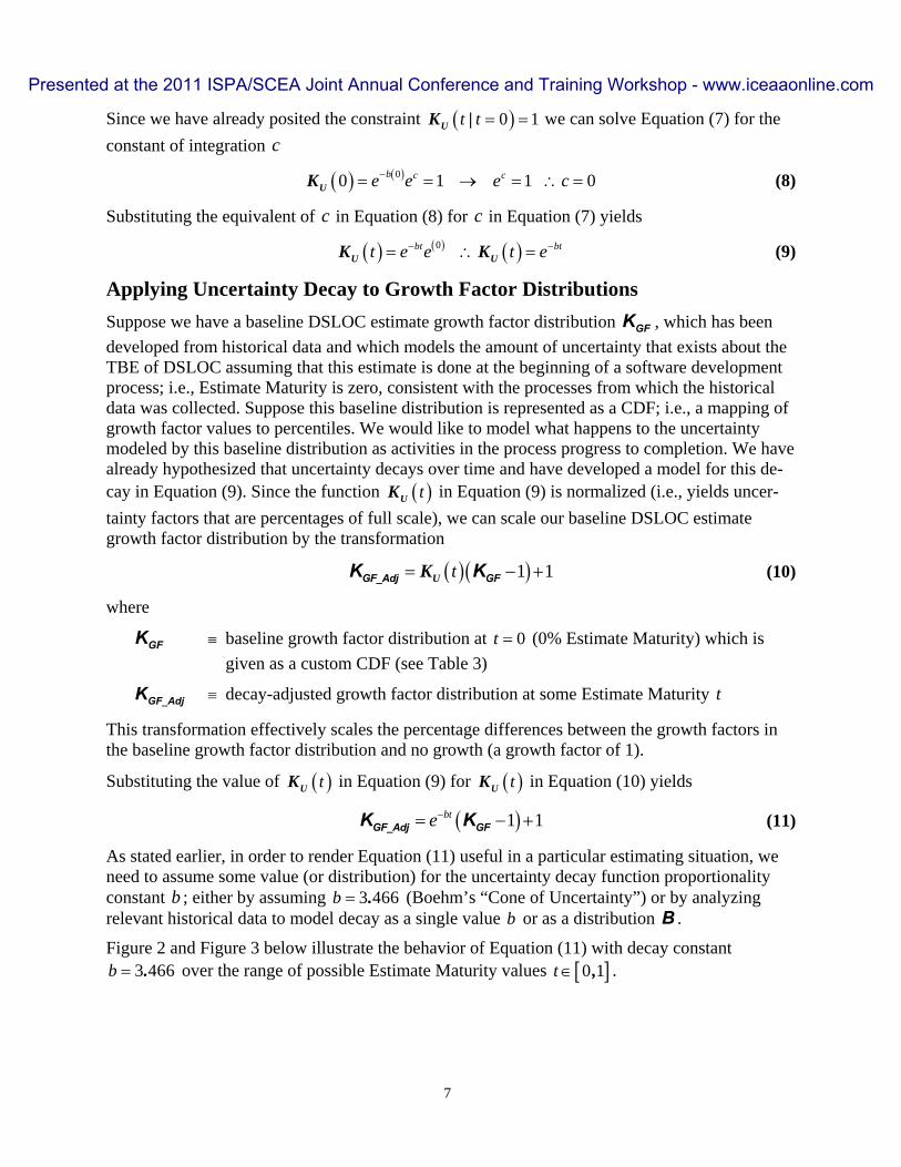
Since we have already posited the constraint 0 1UK |t t we can solve Equation (7) for the

constant of integration c

00 1 1 0UK b c ce e e c (8)

Substituting the equivalent of c in Equation (8) for c in Equation (7) yields

0U UK Kbt btt e e t e (9)

Applying Uncertainty Decay to Growth Factor Distributions

Suppose we have a baseline DSLOC estimate growth factor distribution GFK , which has been

developed from historical data and which models the amount of uncertainty that exists about the TBE of DSLOC assuming that this estimate is done at the beginning of a software development process; i.e., Estimate Maturity is zero, consistent with the processes from which the historical data was collected. Suppose this baseline distribution is represented as a CDF; i.e., a mapping of growth factor values to percentiles. We would like to model what happens to the uncertainty modeled by this baseline distribution as activities in the process progress to completion. We have already hypothesized that uncertainty decays over time and have developed a model for this de-cay in Equation (9). Since the function UK t in Equation (9) is normalized (i.e., yields uncer-

tainty factors that are percentages of full scale), we can scale our baseline DSLOC estimate growth factor distribution by the transformation

1 1UK t GF_Adj GFK K (10)

where

GFK baseline growth factor distribution at 0t (0% Estimate Maturity) which is

given as a custom CDF (see Table 3)

GF_AdjK decay-adjusted growth factor distribution at some Estimate Maturity t

This transformation effectively scales the percentage differences between the growth factors in the baseline growth factor distribution and no growth (a growth factor of 1).

Substituting the value of UK t in Equation (9) for UK t in Equation (10) yields

1 1bte GF_Adj GFK K (11)

As stated earlier, in order to render Equation (11) useful in a particular estimating situation, we need to assume some value (or distribution) for the uncertainty decay function proportionality constant b ; either by assuming 3 466.b (Boehm’s “Cone of Uncertainty”) or by analyzing relevant historical data to model decay as a single value b or as a distribution B .

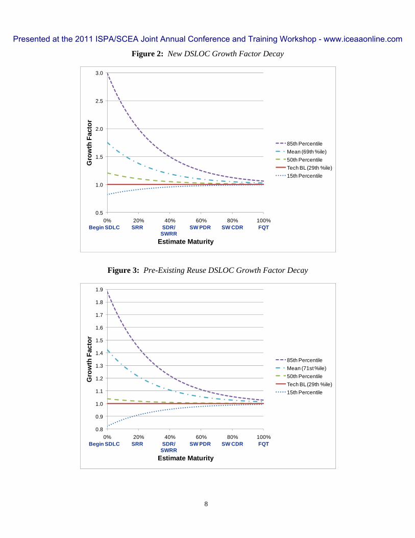
Figure 2 and Figure 3 below illustrate the behavior of Equation (11) with decay constant 3 466.b over the range of possible Estimate Maturity values 0 1,t .


8

Figure 2: New DSLOC Growth Factor Decay

Figure 3: Pre-Existing Reuse DSLOC Growth Factor Decay

0.5

1.0

1.5

2.0

2.5

3.0

0% 20% 40% 60% 80% 100%

Gro

wth

Fac

tor

Estimate Maturity

85th Percentile

Mean (69th %ile)

50th Percentile

Tech BL (29th %ile)

15th Percentile

Begin SDLC SRR SDR/SWRR

SW PDR SW CDR FQT

0.8

0.9

1.0

1.1

1.2

1.3

1.4

1.5

1.6

1.7

1.8

1.9

0% 20% 40% 60% 80% 100%

Gro

wth

Fac

tor

Estimate Maturity

85th Percentile

Mean (71st %ile)

50th Percentile

Tech BL (29th %ile)

15th Percentile


SW PDR SW CDR FQT


9

Applying Growth Factor Distributions to TBEs of New and PER DSLOC

We can now transform single-point TBEs of New D_NewS and PER D_PERS DSLOC into growth-

adjusted distributions of New D_Adj_NewS and PER D_Adj_PERS DSLOC by simply scaling the ap-

propriate instantiation of Equation (11) above (a distribution) by the corresponding single-point TBE:

1 1btD_NewS e D_Adj_New GF_NewS K (12)

and

1 1btD_PERS e D_Adj_PER GF_PERS K (13)

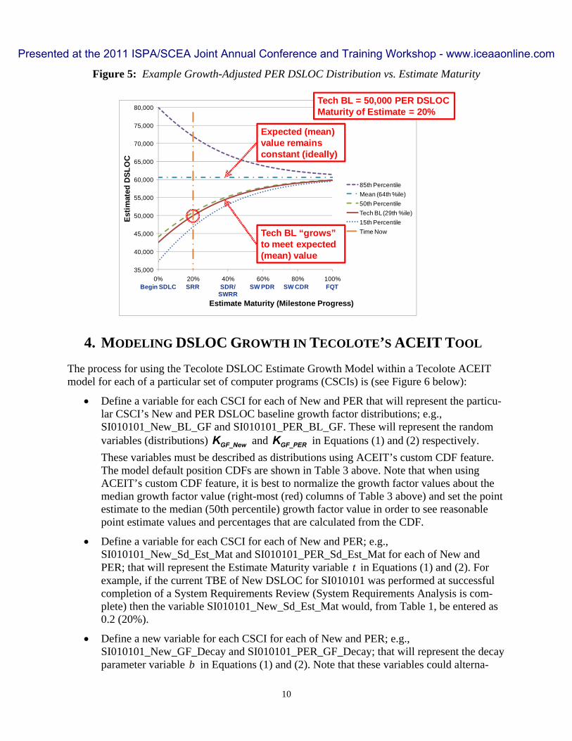
Figure 4 and Figure 5 below illustrate the behaviors of the growth-adjusted New DSLOC esti-mate distribution (Equation (12)) and the growth-adjusted PER DSLOC estimate distribution (Equation (13)) for given New and PER TBEs and a given Estimate Maturity.

Figure 4: Example Growth-Adjusted New DSLOC Distribution vs. Estimate Maturity

15,000

20,000

25,000

30,000

35,000

40,000

45,000

50,000

55,000

60,000

0% 20% 40% 60% 80% 100%

Est

imat

ed D

SL

OC

Estimate Maturity (Milestone Progress)

85th Percentile

Mean (64th %ile)

50th Percentile

Tech BL (29th %ile)

15th Percentile

Time Now

Tech BL = 25,000 New DSLOCMaturity of Estimate = 20%

Tech BL “grows” to meet expected (mean) value

Expected (mean) value remains constant (ideally)


SW PDR SW CDR FQT


10

Figure 5: Example Growth-Adjusted PER DSLOC Distribution vs. Estimate Maturity

4. MODELING DSLOC GROWTH IN TECOLOTE’S ACEIT TOOL

The process for using the Tecolote DSLOC Estimate Growth Model within a Tecolote ACEIT model for each of a particular set of computer programs (CSCIs) is (see Figure 6 below):

Define a variable for each CSCI for each of New and PER that will represent the particu-lar CSCI’s New and PER DSLOC baseline growth factor distributions; e.g., SI010101_New_BL_GF and SI010101_PER_BL_GF. These will represent the random variables (distributions) GF_NewK and GF_PERK in Equations (1) and (2) respectively.

These variables must be described as distributions using ACEIT’s custom CDF feature. The model default position CDFs are shown in Table 3 above. Note that when using ACEIT’s custom CDF feature, it is best to normalize the growth factor values about the median growth factor value (right-most (red) columns of Table 3 above) and set the point estimate to the median (50th percentile) growth factor value in order to see reasonable point estimate values and percentages that are calculated from the CDF.

Define a variable for each CSCI for each of New and PER; e.g., SI010101_New_Sd_Est_Mat and SI010101_PER_Sd_Est_Mat for each of New and PER; that will represent the Estimate Maturity variable t in Equations (1) and (2). For example, if the current TBE of New DSLOC for SI010101 was performed at successful completion of a System Requirements Review (System Requirements Analysis is com-plete) then the variable SI010101_New_Sd_Est_Mat would, from Table 1, be entered as 0.2 (20%).

Define a new variable for each CSCI for each of New and PER; e.g., SI010101_New_GF_Decay and SI010101_PER_GF_Decay; that will represent the decay parameter variable b in Equations (1) and (2). Note that these variables could alterna-

35,000

40,000

45,000

50,000

55,000

60,000

65,000

70,000

75,000

80,000

0% 20% 40% 60% 80% 100%

Est

imat

ed D

SL

OC

Estimate Maturity (Milestone Progress)

85th Percentile

Mean (64th %ile)

50th Percentile

Tech BL (29th %ile)

15th Percentile

Time Now

Tech BL = 50,000 PER DSLOCMaturity of Estimate = 20%

Tech BL “grows” to meet expected (mean) value

Expected (mean) value remains constant (ideally)


SW PDR SW CDR FQT


11

tively be described as a random variables (distributions) B using ACE’s custom CDF feature based on some program-specific historical data. The model default is a constant value for b of 3.466.

Define a variable for each CSCI for each of New and PER; e.g., SI010101_New_Adj_GUF and SI010101_PER_Adj_GUF; that will represent the uncer-tainty-decay-adjusted version of the New DSLOC and PER DSLOC growth factor distri-butions for that CSCI. The equation field for each of these variables implements Equation (11); e.g., exp(–SI010101_New_GF_Decay * SI010101_New_Sd_Est_Mat) * (SI010101_New_BL_GF – 1) + 1.

If the decay constant is being described as a random variable B (distribution) then, be-cause each decay constant random variable is inversely related to its corresponding growth factor random variable, as can be seen in Equation (11), we would need to nega-tively correlate each growth factor / decay constant pair in order for the convolution of these two variables to work properly in ACEIT6. For example, we would group SI010101_New_GF_Decay and SI010101_New_BL_GF and call the group SI010101_Growth_Decay_Group. We would then set the Group Strength of SI010101_New_GF_Decay to “–1” and set the Group Strength of SI010101_New_BL_GF to “D”. Note that none of this step is necessary if using the model defaults based on SRDR data and assuming the decay to be constant with a value of 3.466.

Figure 6: Example ACEIT Model Application of New DSLOC Estimate Growth

5. MODELING DSLOC GROWTH IN GALORATH’S SEER-SEM

TOOL

SEER PERT Distribution

The Galorath, Inc. SEER family of estimating tools incorporate a rather unique probability dis-tribution to model input uncertainty. I refer to this distribution here as a SEER PERT distribu-tion; Program Evaluation and Review Technique (PERT) because it borrows from the mathemat-

6 Note that bte is equivalent to 1 bte .

- New Growth-Adjusted DSLOC SI010101_New_Adj_Sd SI010101_New_Adj_GUF * SI010101_New_Sd- Technical Baseline DSLOC Point Estimate SI010101_New_Sd 25000 [Given]

- Maturity at DSLOC Estimate SI010101_New_Sd_Est_Mat0.20 [Sys Req Rev Complete = 20% Estimate Maturity]

- Baseline Growth Factor SI010101_New_BL_GF

1.204296 [Tecolote DSLOC Estimate Growth Model v06 Median of SRDR New DSLOC Data Set]

- Decay Constant SI010101_New_GF_Decay3.466 [Tecolote DSLOC Estimate Growth Model v06 Default]

- Adjusted Growth Factor SI010101_New_Adj_GUF

exp(-SI010101_New_GF_Decay * SI010101_New_Sd_Est_Mat) * (SI010101_New_BL_GF - 1) + 1 [Tecolote DSLOC Estimate Growth Model v06]


12

ics that the PERT methodology uses to relate elicited expert opinion about the input parameters Least, Likely, and Most. The SEER PERT distribution combines the left half of one Normal (Gaussian) distribution with the right half of another Normal distribution. Because Normal dis-tribution Probability Density Functions (PDFs) are range symmetrical, the mean of the left (low side) half-distribution L is always equal to the mean of the right (high side) half-distribution

H . However, the low side half-distribution standard deviation L need not equal the high-side

half-distribution standard deviation H . When H L the overall SEER PERT distribution is

skewed to the right, when L H the distribution is skewed to the left, and when L H the

distribution is symmetrical and classically Normal. Because the two halves of the distribution are Normal, because each of their means is always equal, and because the mean of a Normal distri-bution is always its median (50th percentile) value, it follows that each half-distribution contains half of the probability density of the overall SEER PERT distribution. Therefore, L and H are

always equal to the overall SEER PERT distribution’s median value %. Note, however, that % is not necessarily equal to the overall SEER PERT distribution’s mean ; this is only true when

L H .

The PDF of the SEER PERT distribution can thus be described as

2

2

2

2

2

2

2 2

2

2

1

2

1

2

SEERf | , ,

L

H

x

L

L Hx

H

e x

x

e x

(14)

the CDF can be described as

2

2 2

2

11

2 2

11

2 2

SEER

erf

F | , ,

erf

L

L H

H

xx

xx

x

(15)

and the inverse CDF (quantile function) can be described as

2 11 2 2

2 1

2 2 1 0 5

2 2 1 0 5

0 1

SEER

erf .F | , ,

erf .

,

LL H

H

p pp

p p

p

(16)

The SEER PERT distribution borrows from PERT methodology in how it relates the distribution parameters %, L , and H to expert opinion elicitations of estimated values that describe a

CSCI’s DSLOC range; these values being referred to as Least L , Likely M , and Most H . The resulting relationships are


13

4

6

L M H

% (17)

and

3L

L

% (18)

and

3H

H

% (19)

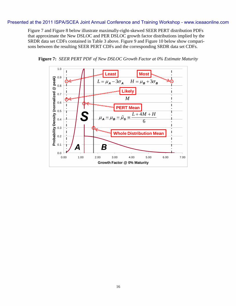
It is important to note here that the PERT relationship in Equation (17) constrains the amount of skew that can be modeled by the SEER PERT distribution. Maximum right (high side) skew occurs when M L and maximum left (low-side) skew occurs when M H . Examples of the SEER PERT PDF can be seen in Figure 7 and Figure 8 below.

Least, Likely, Most Multipliers

SEER-SEM requires that the uncertainty about a DSLOC estimate be characterized as a Least, Likely, Most triple. Since SEER-SEM provides no facility for specifying DSLOC growth and growth uncertainty decay, DSLOC inputs to SEER-SEM must already be growth and uncertainty adjusted. Therefore, in order to model DSLOC growth in SEER-SEM according to the Tecolote DSLOC Estimate Growth Model, DSLOC Least, Likely, and Most values must be chosen that cause SEER-SEM’s SEER PERT distribution to match, as closely as possible, the distributions described in Table 2 and Table 3 and adjusted for uncertainty decay as a function of Estimate Maturity.

Growth-adjusted Least AdjL , Likely AdjM , and Most AdjH DSLOC inputs to SEER-SEM can be

calculated for each of New and PER as functions of the given New and PER DSLOC TBEs

D_NewS and D_PERS with given Estimate Maturity t . For each of New and PER we define a set of

three DSLOC estimate growth multipliers L_AdjK , M_AdjK , and H_AdjK using Equation (11):

3 466 1 1. tL_Adj LK e K (20)

and

3 466 1 1. tM_Adj MK e K (21)

and

3 466 1 1. tH_Adj HK e K (22)

such that

and and_Adj L Adj D Adj M_Adj D Adj H_Adj DL K S M K S H K S (23)

We first instantiate Equations (18), (19) and, (17) with LK , HK , and MK respectively to yield:


14

33

LL L L

KK

%% (24)

and

33

HH H H

KK

%% (25)

and

4 6 3 36

6 4 44 3 3

4

L M H L HL HM M

L HM

K K K K KK K

K

% % %%%

%(26)

Recall that % is always equal to the overall SEER PERT distribution median. We wish to force this value to be equal to the SRDR data set median m%; therefore,

4 3 3

3 and 3 and4

L HL L H H M

mK m K m K

%% % (27)

Substituting the equivalents of LK , HK , and MK in Equations (27) for LK , HK , and MK in

Equations (20), (22), and (21) respectively yields

3 466 3 1 1. tL_Adj LK e m % (28)

and

3 466 4 3 31 1

4. t L H

M_Adj

mK e

% (29)

and

3 466 3 1 1. tH_Adj HK e m % (30)

Appropriate values for m% can be found in Table 2 above. Appropriate values for L and H

have been determined by using the Microsoft Excel Solver add-in to minimize the percentage standard error of estimate %SEE between each SRDR data set CDF and its corresponding SEER PERT CDF varying L and H . The results from running Solver and then calculating LK , MK ,

and HK are shown in Table 4 below.


15

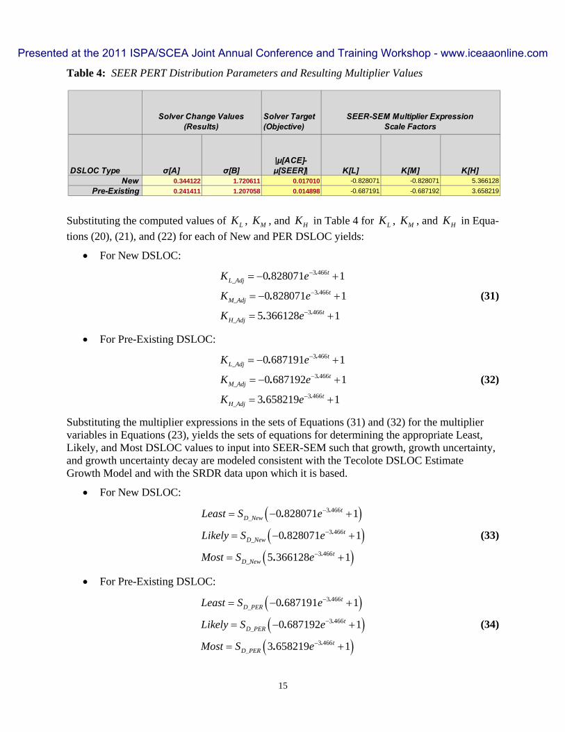
Table 4: SEER PERT Distribution Parameters and Resulting Multiplier Values

Substituting the computed values of LK , MK , and HK in Table 4 for LK , MK , and HK in Equa-

tions (20), (21), and (22) for each of New and PER DSLOC yields:

For New DSLOC:

3 466

3 466

3 466

0 828071 1

0 828071 1

5 366128 1

.

.

.

.

.

.

tL_Adj

tM_Adj

tH_Adj

K e

K e

K e

(31)

For Pre-Existing DSLOC:

3 466

3 466

3 466

0 687191 1

0 687192 1

3 658219 1

.

.

.

.

.

.

tL_Adj

tM_Adj

tH_Adj

K e

K e

K e

(32)

Substituting the multiplier expressions in the sets of Equations (31) and (32) for the multiplier variables in Equations (23), yields the sets of equations for determining the appropriate Least, Likely, and Most DSLOC values to input into SEER-SEM such that growth, growth uncertainty, and growth uncertainty decay are modeled consistent with the Tecolote DSLOC Estimate Growth Model and with the SRDR data upon which it is based.

For New DSLOC:

3 466

3 466

3 466

0 828071 1

0 828071 1

5 366128 1

.

.

.

.

.

.

tD_New

tD_New

tD_New

Least S e

Likely S e

Most S e

(33)

For Pre-Existing DSLOC:

3 466

3 466

3 466

0 687191 1

0 687192 1

3 658219 1

.

.

.

.

.

.

tD_PER

tD_PER

tD_PER

Least S e

Likely S e

Most S e

(34)

Solver Target (Objective)

DSLOC Type σ[A] σ[B]|μ[ACE]-μ[SEER]| K[L] K[M] K[H]

New 0.344122 1.720611 0.017010 -0.828071 -0.828071 5.366128

Pre-Existing 0.241411 1.207058 0.014898 -0.687191 -0.687192 3.658219

Solver Change Values (Results)

SEER-SEM Multiplier ExpressionScale Factors


16

Figure 7 and Figure 8 below illustrate maximally-right-skewed SEER PERT distribution PDFs that approximate the New DSLOC and PER DSLOC growth factor distributions implied by the SRDR data set CDFs contained in Table 3 above. Figure 9 and Figure 10 below show compari-sons between the resulting SEER PERT CDFs and the corresponding SRDR data set CDFs.

Figure 7: SEER PERT PDF of New DSLOC Growth Factor at 0% Estimate Maturity

0.0

0.1

0.2

0.3

0.4

0.5

0.6

0.7

0.8

0.9

1.0

0.00 1.00 2.00 3.00 4.00 5.00 6.00 7.00

Pro

bab

ilit

y D

ensi

ty (

no

rmal

ized

@ p

eak)

Growth Factor @ 0% Maturity

A B

S

Least Most

Likely

PERT Mean

M

4

6

L M H A B S

Whole Distribution Mean

L 3L A A H 3H B B


17

Figure 8: SEER PERT PDF of PER DSLOC Growth Factor at 0% Estimate Maturity

Figure 9: Comparison of New DSLOC Growth Factor CDFs – SEER PERT vs. SRDR Data

0.0

0.1

0.2

0.3

0.4

0.5

0.6

0.7

0.8

0.9

1.0

0.00 0.50 1.00 1.50 2.00 2.50 3.00 3.50 4.00 4.50 5.00

Pro

bab

ilit

y D

ensi

ty (

no

rmal

ized

@ p

eak)

Growth Factor @ 0% Maturity

A B

S

Least Most

3L A A 3H B B

Likely

PERT Mean

M

4

6

L M H A B S

Whole Distribution Mean

1 372307. S S

0

10

20

30

40

50

60

70

80

90

100

0 1 2 3 4 5 6 7

Per

cen

tile

New DSLOC Growth Factor

Tech BL

SRDR CDF

SRDR Mean

SEER CDF

SEER Mean

Maturity of Estimate = 0%

Mean Growth Factor Value:1.75 (SRDR Data)1.75 (SEER PERT Approx)

Mean Confidence %:69% (SRDR Data)63% (SEER PERT Approx)


18

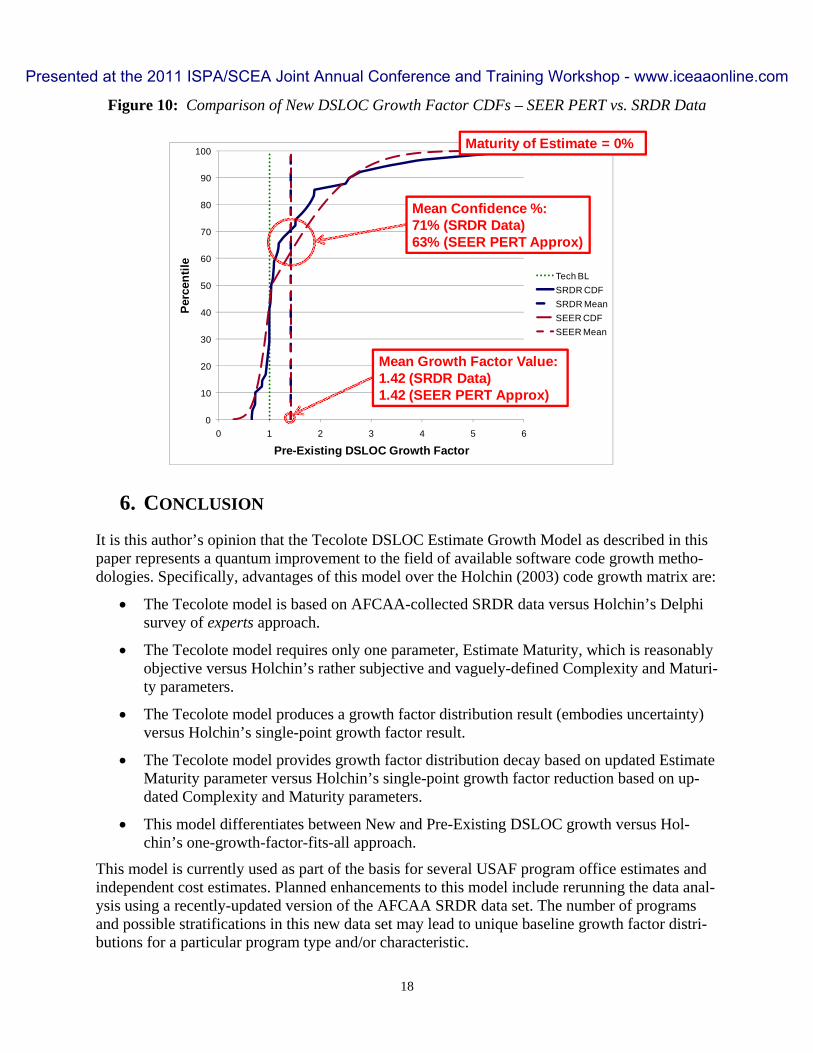
Figure 10: Comparison of New DSLOC Growth Factor CDFs – SEER PERT vs. SRDR Data

6. CONCLUSION

It is this author’s opinion that the Tecolote DSLOC Estimate Growth Model as described in this paper represents a quantum improvement to the field of available software code growth metho-dologies. Specifically, advantages of this model over the Holchin (2003) code growth matrix are:

The Tecolote model is based on AFCAA-collected SRDR data versus Holchin’s Delphi survey of experts approach.

The Tecolote model requires only one parameter, Estimate Maturity, which is reasonably objective versus Holchin’s rather subjective and vaguely-defined Complexity and Maturi-ty parameters.

The Tecolote model produces a growth factor distribution result (embodies uncertainty) versus Holchin’s single-point growth factor result.

The Tecolote model provides growth factor distribution decay based on updated Estimate Maturity parameter versus Holchin’s single-point growth factor reduction based on up-dated Complexity and Maturity parameters.

This model differentiates between New and Pre-Existing DSLOC growth versus Hol-chin’s one-growth-factor-fits-all approach.

This model is currently used as part of the basis for several USAF program office estimates and independent cost estimates. Planned enhancements to this model include rerunning the data anal-ysis using a recently-updated version of the AFCAA SRDR data set. The number of programs and possible stratifications in this new data set may lead to unique baseline growth factor distri-butions for a particular program type and/or characteristic.

0

10

20

30

40

50

60

70

80

90

100

0 1 2 3 4 5 6

Per

cen

tile

Pre-Existing DSLOC Growth Factor

Tech BL

SRDR CDF

SRDR Mean

SEER CDF

SEER Mean

Maturity of Estimate = 0%

Mean Growth Factor Value:1.42 (SRDR Data)1.42 (SEER PERT Approx)

Mean Confidence %:71% (SRDR Data)63% (SEER PERT Approx)


19

REFERENCES

Boehm, Barry W. 1981. Software Engineering Economics. Englewood Cliffs : Prentice-Hall, Inc., 1981. ISBN 0-13-822122-7.

Holchin, Barry. 2003. Code Growth Study. September 17, 2003.


20

BIOGRAPHY

Michael A. Ross has over 35 years of experience in software engineering as a developer, man-ager, process expert, consultant, instructor, and award-winning international speaker. Mr. Ross is currently a Technical Expert for Tecolote Research, Inc. Mr. Ross’s previous experience includes three years as President and CEO of r2Estimating, LLC (makers of the r2Estimator software estimation tool), three years as Chief Scientist of Galorath Inc. (makers of the SEER suite of estima-tion tools), seven years with Quantitative Software Management, Inc. (makers of the SLIM suite of software estimating tools) where he was a senior consul-

tant and Vice President of Education Services, and 17 years with Honeywell Air Transport Sys-tems (formerly Sperry Flight Systems) and 2 years with Tracor Aerospace where he developed and/or managed the development of real-time embedded software for various military and com-mercial avionics systems. Mr. Ross did his undergraduate work at the United States Air Force Academy and Arizona State University, receiving a Bachelor of Science in Computer Engineer-ing.


Presented at the 2011 ISPA/SCEA Joint Annual Conference ... · An Improved Method for Predicting...

Documents

Transcript of Presented at the 2011 ISPA/SCEA Joint Annual Conference ... · An Improved Method for Predicting...