PRESENTATION OF AFFINE KAC-MOODY GROUPSOVER RINGS

DANIEL ALLCOCK

Abstract. Tits has defined Steinberg groups and Kac-Moodygroups for any root system and any commutative ring R. We es-tablish a Curtis-Tits-style presentation for the Steinberg group Stof any rank ≥ 3 irreducible affine root system, for any R. Namely,St is the direct limit of the Steinberg groups coming from the 1-and 2-node subdiagrams of the Dynkin diagram. This leads to acompletely explicit presentation. Using this we show that St isfinitely presented if the rank is ≥ 4 and R is finitely generated as aring, or if the rank is 3 and R is finitely generated as a module overa subring generated by finitely many units. Similar results hold forthe corresponding Kac-Moody groups when R is a Dedekind do-main of arithmetic type.

1. Introduction

Suppose R is a commutative ring and A is one of the ABCDEFGDynkin diagrams, or equivalently its Cartan matrix. Steinberg de-fined what is now called the Steinberg group StA(R), by generatorsand relations [18]. It plays a central role in K-theory and some aspectsof Lie theory.

Kac-Moody algebras are infinite-dimensional generalizations of thesemisimple Lie algebras. When R = R and A is an irreducible affineDynkin diagram, the corresponding Kac-Moody group is a central ex-tension of the loop group of a finite-dimensional Lie group. For ageneral ring R and any generalized Cartan matrix A, the definitionof the Kac-Moody group is due to Tits [20]. He first constructed agroup functor R 7→ StA(R) generalizing Steinberg’s, also by genera-

tors and relations. Then he defined another functor R 7→ GA(R) asa certain quotient of this. In this paper we will omit the tilde andrefer to GA(R) as the Kac-Moody group of type A over R. (Tits ac-

tually defined GD(R) where D is a root datum; by GA(R) we intend

Date: September 23, 2014.2000 Mathematics Subject Classification. Primary: 20G44; Secondary: 14L15,

22E67, 19C99.Supported by NSF grant DMS-1101566.

1

2 DANIEL ALLCOCK

the root datum whose generalized Cartan matrix is A and which is“simply-connected in the strong sense” [20, p. 551].)

The meaning of “Kac-Moody group” is far from standardized. In [20]Tits wrote down axioms (KMG1)–(KMG9) that one could demand ofa functor from rings to groups before calling it a Kac-Moody func-tor. He showed [20, Thm. 1′] that any such functor admits a naturalhomomorphism from GA, which is an isomorphism at every field. SoKac-Moody groups over fields are well-defined, and over general ringsGA approximates the yet-unknown ultimate definition. This is why werefer to GA as the Kac-Moody group. But GA does not quite satisfyTits’ axioms, so ultimately some other language may be better. Seesection 5 for more remarks on this.

The purpose of this paper is to simplify Tits’ presentations of StA(R)and GA(R) when A is an irreducible affine Dynkin diagram of rank(number of nodes) at least 3. In particular, we show that these groupsare finitely presented under quite weak hypotheses on R. This is sur-prising because there is no obvious reason for an infinite-dimensionalgroup over (say) Z to be finitely presented, and Tits’ presentations are“very” infinite. His generators are indexed by all pairs (root, ring el-ement), and his relations specify the commutators of certain pairs ofthese generators. Subtle implicitly-defined coefficients appear through-out his relations.

To prove our finite presentation results, we will first establish explicitpresentations for StA(R) and GA(R) that are much smaller than Tits’presentations, though still infinite if R is infinite. Namely, in [2] wedefined for any A a group functor we called the pre-Steinberg groupPStA. The definition is the same as Tits’ definition of StA, as modifiedby Morita-Rehmann [14], except with some relations omitted. Themain result of this paper is that the omitted relations are redundant.More formally, theorem 1 states that PStA → StA is an isomorphism.This is useful because in [2, thm. 1.2] we gave a simple closed-formpresentation of PStA.

This presentation has generators Si and Xi(t), with i varying overthe nodes of the Dynkin diagram and t over R, and the relations are(70)–(95) in [2]. A full list of the relations is not needed in this paper,but for concreteness we give in table 1 the complete presentation whenA is simply-laced (and not A1). If multiple bonds are present then therelations are more complicated but similar. Or see [2, sec. 2] for theA1, A2, B2 and G2 cases, which are enough to present PStA(R) forany A.

PRESENTATION OF AFFINE KAC-MOODY GROUPS OVER RINGS 3

Xi(t)Xi(u) = Xi(t+ u)

[S2i , Xi(t)] = 1

Si = Xi(1)SiXi(1)S−1i Xi(1)

all i

SiSj = SjSi

[Si, Xj(t)] = 1

[Xi(t), Xj(u)] = 1

all unjoined i 6= j

SiSjSi = SjSiSj

S2i SjS

−2i = S−1

j

Xi(t)SjSi = SjSiXj(t)

S2iXj(t)S

−2i = Xj(t)

−1

[Xi(t), SiXj(u)S−1i ] = 1

[Xi(t), Xj(u)] = SiXj(tu)S−1i

all joined i 6= j

Table 1. Defining relations for PStA(R) when A issimply-laced. The generators are Xi(t) and Si where ivaries over the nodes of the Dynkin diagram and t over R.When A is also affine, this also presents StA(R), by the-orem 1.

Theorem 1 (Presentation of affine Steinberg and Kac-Moody groups).Suppose A is an irreducible affine Dynkin diagram of rank ≥ 3 and Ris a commutative ring. Then the natural map PStA(R) → StA(R) isan isomorphism.

In particular, StA(R) has a presentation with generators Si andXi(t), with i varying over the simple roots and t over R, and relators(70)–(95) from [2]. (Or see table 1 when A is simply-laced.)

One obtains GA(R) by adjoining the relations

(1) hi(u)hi(v) = hi(uv)

for every simple root i and all units u, v of R, where

si(u) := Xi(u)SiXi(1/u)S−1i Xi(u)

hi(u) := si(u)si(−1).

We remark that if A is a spherical diagram (that is, its Weyl groupis finite) then PStA → StA is an isomorphism, essentially by thedefinition of PStA. See [2] for details. So theorem 1 extends theisomorphism PStA

∼= StA to the irreducible affine case (except for

4 DANIEL ALLCOCK

rank 2). See [3] for a further extension, to the simply-laced hyperboliccase.

The key property of our presentation of PStA(R) is its description interms of the Dynkin diagram rather than the full (usually infinite) rootsystem, as in Tits’ construction. Furthermore, every relation involvesjust one or two subscripts. In the simply-laced case one can check thisby examining table 1, and in the general case one examines the relators(70)–(95) in [2]. Also, the extra relations (1) needed to define the Kac-Moody group also involve only single subscripts. Therefore we obtainthe following corollary:

Corollary 2 (Curtis-Tits presentation). Suppose A is an irreducibleaffine Dynkin diagram of rank ≥ 3 and R is a commutative ring. Con-sider the groups StB(R) and the obvious maps between them, as Bvaries over the singletons and pairs of nodes of A. The direct limit ofthis family of groups equals StA(R).

The same result holds with St replaced by G throughout. �

A consequence of the corollary 2 is that StA(R)’s presentation canbe got by gathering together the presentations for the StB(R)’s. Whenthe latter groups are finitely presented, we can therefore expect thatStA(R) is too. The finite presentability of StB(R) was examined bySplitthoff [17]. Using his work and some additional arguments, weobtain the following:

Theorem 3 (Finite presentability). Suppose A is an irreducible affineDynkin diagram of rank ≥ 3 and R is a commutative ring. ThenStA(R) is finitely presented if either

(i) rkA > 3 and R is finitely generated as a ring, or(ii) rkA ≥ 3 and R is finitely generated as a module over a subring

generated by finitely many units.

In either case, if the unit group of R is finitely generated as an abeliangroup, then GA(R) is also finitely presented.

One of the main motivations for Splitthoff’s work was to understandwhether the Chevalley-Demazure groups over Dedekind domains of in-terest in number theory, are finitely presented. This was settled byBehr [5][6], capping a long series of works by many authors. The fol-lowing analogue of these results follows immediately from theorem 3.How close the analogy is depends on how well GA approximates what-ever plays the role of the Chevalley-Demazure group scheme in thesetting of Kac-Moody algebras.

PRESENTATION OF AFFINE KAC-MOODY GROUPS OVER RINGS 5

Corollary 4 (Finite presentation in arithmetic contexts). Suppose Kis a global field, meaning a finite extension of Q or Fq(t). Suppose Sis a nonempty finite set of places of K, including all infinite places inthe number field case. Let R be the ring of S-integers in K.

Suppose A is an irreducible affine Dynkin diagram. Then Tits’ Kac-Moody group GA(R) is finitely presented if

(i) rkA > 3 when K is a function field and |S| = 1;(ii) rkA ≥ 3 otherwise. �

In a companion paper with Carbone [3] we prove analogues of allfour theorems for the simply-laced hyperbolic Dynkin diagrams, suchas E10.

We remark that if R is a field then the GA case of corollary 2 is dueto Abramenko-Muhlherr [1][15]. Namely, suppose A is any generalizedCartan matrix which is 2-spherical (its Dynkin diagram has no edgeslabeled ∞), and that R is a field (but not F2 if A has a double bond,and neither F2 nor F3 if A has a multiple bond). Then GA(R) is thedirect limit of the groups GB(R). See also Caprace [8]. Abramenko-Muhlherr [1, p. 702] state that if A is irreducible affine then one canremove the restrictions R 6= F2,F3.

One of our goals in this work is to bring Kac-Moody groups intothe world of geometric and combinatorial group theory, which mostlyaddresses finitely presented groups. For example: which Kac-Moodygroups admit classifying spaces with finitely many cells below somechosen dimension? What other finiteness properties do they have? Dothey have Kazhdan’s property T? What isoperimetric inequalities dothey satisfy in various dimensions? Are there (non-split) Kac-Moodygroups over local fields whose uniform lattices (suitably defined) areword hyperbolic? Are some Kac-Moody groups (or classes of them)quasi-isometrically rigid? We find the last question very attractive,since the corresponding answer [9][10][13][16] for lattices in Lie groupsis deep.

The author is very grateful to the Japan Society for the Promotionof Science and to Kyoto University, for their support and hospitality.He would also like to thank Lisa Carbone for useful comments on andraft version of the paper.

2. Steinberg and pre-Steinberg Groups

We work in the setting of [20] and [2], so R is a commutative ring andA is a generalized Cartan matrix. This matrix determines a complexLie algebra g = gA called the Kac-Moody algebra, and we write Φ forthe set of real roots of g. Tits’ definition of the Steinberg group StA(R)

6 DANIEL ALLCOCK

starts with the free product ∗α∈Φ Uα, where each root group Uα is acopy of the additive group of R.

Tits calls a pair α, β ∈ Φ prenilpotent if some element of the Weylgroup W sends both α, β to positive roots, and some other element ofW sends both to negative roots. A consequence of this condition isthat every root in Nα + Nβ is real, which enabled Tits to write downChevalley-style relators for α, β. That is, for every prenilpotent pairα, β he imposes relations of the form

(2)[element of Uα, element of Uβ

]=

∏γ∈θ(α,β)−{α,β}

(element of Uγ)

where θ(α, β) := (Nα + Nβ) ∩ Φ and N = {0, 1, 2, . . . }. In the generalcase, the exact relations are given in a rather implicit form in [20, §3.6].We give them explicitly in section 4, but only in the cases we need andonly as we need them. For Tits, and for purposes of this paper, this isthe end of the definition of StA(R).

The pre-Steinberg group PStA(R), defined in [2, sec. 7], imposesthese relations only for the classically nilpotent pairs α, β. This meansthat α, β are linearly independent and (Qα ⊕ Qβ) ∩ Φ is finite. Thisis equivalent to α, β being non-antipodal and lying in some A2

1, A2,B2 or G2 root system. As the name suggests, such a pair is prenilpo-tent. So PStA(R) is defined the same way as StA(R), just omittingthe Chevalley relations for prenilpotent pairs that are not classicallyprenilpotent. In particular, StA(R) is a quotient of PStA(R), hencethe prefix “pre-”.

There are some additional relations in the pre-Steinberg group, andin the Steinberg group as defined by Morita-Rehmann [14], whom wefollow. These relations are natural, and required to recover Steinberg’soriginal definition in the A1 case. But they are irrelevant to this pa-per. This is because they follow from the relations in PStA(R) thatwe have already described, whenever A is 2-spherical without A1 com-ponents. So we will make only the following remarks. First, the extrarelations are labeled (69) in [2] and (B′) in [14, p. 538]. Second, Titsimposed them when defining the Kac-Moody group GA(R) as a quo-tient of StA(R), in [20, eqn. (6)]. Third, Tits’ remark (a) in [20, p. 549]explains why they follow from the relations in PStA(R).

We have not really defined StA(R) and PStA(R), just discussed thegeneral form of the definitions. The reason is that there are delicatesigns present that are not important in this paper. This has nothing todo with Kac-Moody theory and is already present in Steinberg’s origi-nal groups. Tits’ description of the relations (2) elegantly circumvents

PRESENTATION OF AFFINE KAC-MOODY GROUPS OVER RINGS 7

this problem, but at the cost of making all the relations implicit ratherthan explicit.

One reason we introduced PStA is that we could write down a com-pletely explicit presentation for it. The philosophy is that in many casesof interest, the natural map PStA(R)→ StA(R) is an isomorphism. Infact we presume that PStA is interesting only when this isomorphismholds. When it does, we get the completely explicit presentation ofStA referred to in theorem 1. Its fine details are unimportant in thispaper.

3. New nomenclature for affine root systems

Our proof of theorem 1, appearing in the next section, refers to theroot system as a whole, with the simple roots playing no special role.It is natural in this setting to use a nomenclature for the affine rootsystems that emphasizes this global perspective.

The names we use are An, . . . , G2, B evenn , C even

n , F even4 , G 0 mod 3

2 and

BC oddn . Their virtues are: the subscript is the rank (minus 1, as usual),

the corresponding finite root system is indicated by the capital letter(s),

and the construction of X ···n is visible in the superscript. We now givethe constructions along with the correspondence with Kac’s nomencla-ture [12, pp. 54–55].

Suppose Φ is a root system of type Xn = An≥1, Bn≥2, Cn≥2, Dn≥2,E6,7,8, F4 or G2, and Λ is its root lattice. We define the root system Φ

of type Xn as Φ×Z ⊆ Λ := Λ⊕Z. It corresponds to Kac’s X(1)n . This

can be seen by taking simple roots for Φ and adjoining (α, 1) where αis the lowest long root of Φ.

For Xn = Bn, Cn or F4 we define X evenn as the set of (α,m) ∈ Xn such

that m ≡ 0 mod 2 if α is long. These correspond to Kac’s D(2)n+1, A

(2)2n−1

and E(2)6 respectively. This can be seen as in the previous paragraph,

using the lowest short root instead of the lowest long root.

We define G 0 mod 32 by the same construction, with the condition m ≡

0 mod 2 replaced by m ≡ 0 mod 3. This corresponds to Kac’s D(3)4 , by

the same recipe as the previous paragraph.For the last affine root system we recall that BCn≥2 is the union of

the Bn and Cn root systems. It is non-reduced and has 3 lengths ofroots, called short, middling and long. Taking Φ = BCn, we define the

root system Φ of type BC oddn as the set of all (α,m) ∈ Φ×Z such that

m is odd if α is long. Although Φ is non-reduced, Φ is reduced because

of this parity condition. Kac’s notation is A(2)2n . To check this, begin

with the set of roots in BC oddn having m = 0, which has type Bn, take

8 DANIEL ALLCOCK

simple roots for it, and adjoin (2α, 1) where α is the lowest short root

of Bn. The Dynkin diagram of these roots is then Kac’s A(2)2n .

In all cases, the root system of type X ···n is the set of pairs (root of Xn,m ∈ Z), satisfying the condition that if the root is long then m has theproperty indicated in the superscript.

4. The isomorphism PStA(R)→ StA(R)

This section is devoted to proving theorem 1, whose hypotheses weassume throughout. Our goal is to show that the Chevalley relationsfor the classically prenilpotent pairs imply those of the remaining pre-nilpotent pairs. We will begin by saying which pairs of real roots areprenilpotent and which are classically prenilpotent. Then we will ana-lyze the pairs that are prenilpotent but not classically prenilpotent.

We fix the affine Dynkin diagram A, write Φ,Φ,Λ,Λ as in section 3,and use an overbar to indicate projections of roots from Φ to Φ. Itis easy to see that α, β ∈ Φ are classically prenilpotent just if theirprojections α, β ∈ Φ are linearly independent. The following lemmadescribes which pairs of roots are prenilpotent but not classically pre-nilpotent, and what their Chevalley relations are (except for one specialcase discussed later).

Lemma 5. Suppose α, β ∈ Φ are distinct. Then the following areequivalent:

(i) α, β are prenilpotent but not classically prenilpotent;(ii) α, β differ by a positive scalar factor;

(iii) α, β are equal, or one is twice the other and Φ = BC oddn .

When these equivalent conditions hold, the Chevalley relations betweenUα,Uβ in Tits’ definition of StA(R) are [Uα,Uβ] = 1, unless Φ =

BC oddn , α and β are the same short root of Φ = BCn, and α + β ∈ Φ.

Proof. Recall that two roots α, β ∈ Φ form a prenilpotent pair if someelement of the affine Weyl group W sends both to positive roots, andsome other element of W sends both to negative roots. We gave simpleroots for Φ in section 3, including a choice of simple roots for the subsetΦ0 having m = 0. With respect to these, α = (α,m) ∈ Φ is positivejust if either m > 0, or m = 0 and α is positive in Φ0.

The “translation” part of the affine Weyl group acts on Φ by shears(α,m) 7→ (α,m+ φ(α)), with φ a linear function Λ→ Z. The set of φoccurring in this way is a subgroup of finite index in Hom(Λ,Z). Thismakes it easy to see that if α, β are linearly independent, then someshear in W sends α, β to positive roots, and another one sends them

PRESENTATION OF AFFINE KAC-MOODY GROUPS OVER RINGS 9

to negative roots. The same argument works if α, β differ by a positivescalar factor. So α, β are prenilpotent in these cases.

If α, β differ by a negative scalar factor then some positive linearcombination of α, β has the form (0,m). The affine Weyl group actstrivially on the second summand in Λ = Λ ⊕ Z. It follows that ifsome element of W sends α, β to positive (resp. negative) roots, thenm is positive (resp. negative). Since m cannot be both positive andnegative, α, β cannot be a prenilpotent pair.

We have shown that α, β ∈ Φ fail to be prenilpotent just if α, βare negative multiples of each other. We remarked above that α, βare classically prenilpotent just if α, β are linearly independent. Thisproves the equivalence of (i) and (ii). To see the equivalence of (ii)and (iii) we refer to the fact that Φ is a reduced root system (i.e, theonly positive multiple of a root that can be a root is that root itself)

except in the case Φ = BC oddn . In this last case, the only way one root

of Φ = BCn can be a positive multiple of a different root is that thelong roots are got by doubling the short roots.

The proof of the final claim is similar. Except in the excluded case,we have Φ ∩ (Nα + Nβ) = {α, β}. The corresponding claim for Φfollows, so θ(α, β) − {α, β} is empty and the right hand side of (2) isthe identity. That is, the Chevalley relations for α, β read [Uα,Uβ] = 1.(In the excluded case we remark that Φ ∩ (Nα + Nβ) = {α, β, α + β}.So the Chevalley relations set the commutators of elements of Uα withelements of Uβ equal to certain elements of Uα+β. See case 6 below.) �

Recall that PStA(R) is defined by the Chevalley relations of theclassically prenilpotent pairs, and StA(R) by those of all prenilpotentpairs. So to prove theorem 1 it suffices to show that if α, β are pre-nilpotent but not classically prenilpotent, then their Chevalley relationsalready hold in PSt := PStA(R).

The cases we must address are given in the lemma above, and inevery case but one we must establish [Uα,Uβ] = 1. Each case begins bychoosing two roots in Φ, of which β is a specified linear combination,and whose projections to Φ are specified. Given the global descriptionof Φ from section 3, this is always easy. Then we use the Chevalleyrelations for various classically prenilpotent pairs to deduce the Cheval-ley relations for α, β. When necessary we refer to [2, (79)–(92)] for theexact forms of the Chevalley relations.

The proof of theorem 1 now falls into seven cases, according to Φand the relative position of α and β.

10 DANIEL ALLCOCK

Case 1 of theorem 1. Assume α = β is a root of Φ = An≥2, Dn orEn, or a long root of Φ = G2. Choose γ, δ ∈ Φ as shown, and chooselifts γ, δ ∈ Φ summing to β. (Choose any γ ∈ Φ lying over γ, defineδ = β − γ, and use the global description of Φ to check that δ ∈ Φ.

This is trivial except in the case Φ = G 0 mod 32 , when it is easy.)

γ

α, β

δ

Because α + γ, α + δ /∈ Φ, it follows that α + γ, α + δ /∈ Φ. So theChevalley relations [Uα,Uγ] = [Uα,Uδ] = 1 hold. The Chevalley re-lations for γ, δ imply [Uγ,Uδ] = Uγ+δ = Uβ. (These relations are [2,(89)] in the G2 case and [2, (81)] in the others. One can write them as[Xγ(t), Xδ] = Xγ+δ(tu) in the notation of the next paragraph.) SinceUα commutes with Uγ and Uδ, it also commutes with Uβ, as desired. �

The other cases use the same strategy: express an element of Uβ interms of other root groups, and then evaluate its commutator with anelement of Uα. But the calculations are more delicate. We will workwith explicit elements Xγ(t) ∈ Uγ for various roots γ ∈ Φ. Here t variesover R, and the definition of Xγ(t) depends on a choice of basis vectoreγ for the corresponding root space gγ ⊆ g. One should think of Xγ(t)as “exp(teγ)”. Following Tits [20, §3.3], there are two equally canonicalchoices for eγ, differing by a sign. Changing one’s choice correspondsto negating t. This choice of sign is irrelevant to the arguments below,except that a choice is required in order to write down the relationsexplicitly.

The Chevalley relations in [2] are given in a form originally due toDemazure. For example, if λ, σ are long and short simple roots for aB2 root system, then their relations are given in [2, (85)] as

(3) [Xσ(t), Xλ(u)] · SσXλ(−t2u)S−1σ · SλXσ(tu)S−1

λ = 1,

for all t, u ∈ R. The advantage of this form is technical: to writedown the relation, one only needs to specify generators for gσ and gλ,not the other root spaces involved. But for explicit computation onemust choose generators for these other root spaces. Because Sσ andSλ permute the root spaces by the reflections in σ and λ, the secondand third terms in (3) lie in Uλ+2σ and Uλ+σ respectively. Therefore,after choosing suitable generators eλ+2σ and eλ+σ for gλ+2σ and gλ+σ,we may rewrite (3) as

(4) [Xσ(t), Xλ(u)] ·Xλ+2σ(−t2u) ·Xλ+σ(tu) = 1.

PRESENTATION OF AFFINE KAC-MOODY GROUPS OVER RINGS 11

We could just as well replace eλ+2σ (resp. eλ+σ) by its negative; thenwe would also replace −t2u (resp. tu) by its negative.

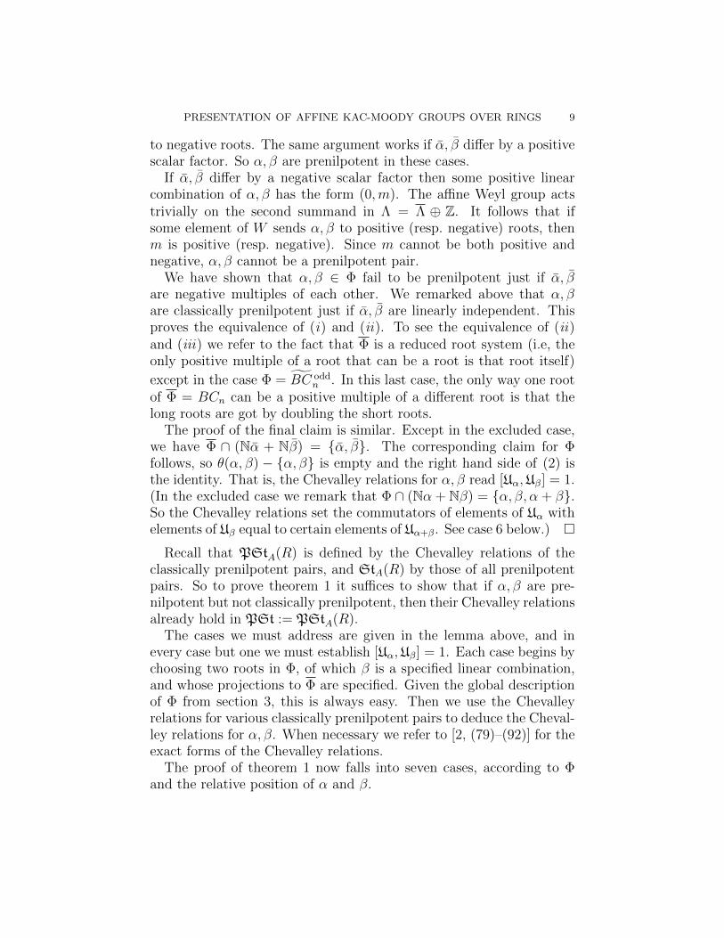
Case 2 of theorem 1. Assume α = β is a long root of Φ = Bn≥2, Cn≥2,BCn≥2 or F4. Our first step is to choose roots λ, σ ∈ Φ as pictured:

λ α, β

σ

This is easily done using any standard description of Φ. (Note: al-though λ stands for “long” and σ for “short”, σ is actually a middlingroot in the case Φ = BCn.)

Our second step is to choose lifts λ, σ ∈ Φ of them with β = λ+ 2σ.

If Φ = Bn, Cn or F 4 then one chooses any lift σ of σ and definesλ as β − 2σ. This works since every element of Λ lying over a root

of Φ is a root of Φ. If Φ = B evenn , C even

n , F even4 or BC odd

n then thisargument might fail since Φ is “missing” some long roots. Instead,one chooses any λ ∈ Φ lying over λ and defines σ as (β − λ)/2. Now,β − λ = (β − λ,m) with the second entry being even by the meaningof the superscript even or odd. Also, β − λ is divisible by 2 in Λ by thefigure above. It follows that σ ∈ Λ. Then, as an element of Λ lyingover a short (or middling) root of Φ, σ lies in Φ.

Because σ, λ are simple roots for a B2 root system inside Φ, theirChevalley relation (4) holds in PSt. It shows that any element ofUβ = Uλ+2σ can be written in the form

(5)[(some xλ ∈ Uλ), (some xσ ∈ Uσ)

]· (some xλ+σ ∈ Uλ+σ).

Referring to the picture of Φ shows that α + λ /∈ Φ. Therefore theChevalley relations in PSt include [Uα,Uλ] = 1. In particular, Uαcommutes with the first term in the commutator in (5). The sameargument shows that Uα also commutes with the other terms. Thisshows that the Chevalley relations present in PSt imply [Uα,Uβ] = 1,as desired. �

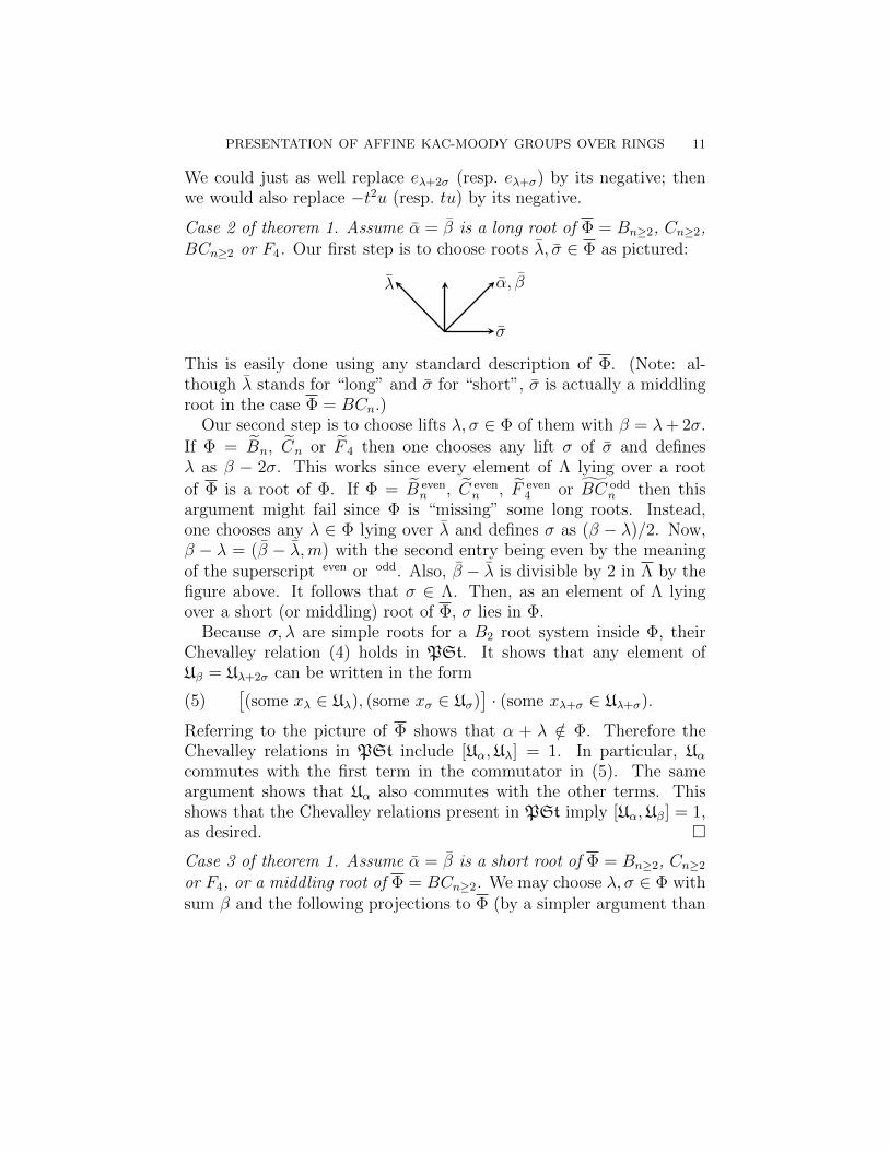
Case 3 of theorem 1. Assume α = β is a short root of Φ = Bn≥2, Cn≥2

or F4, or a middling root of Φ = BCn≥2. We may choose λ, σ ∈ Φ withsum β and the following projections to Φ (by a simpler argument than

12 DANIEL ALLCOCK

in the previous case):

λα, β

σ

The Chevalley relations for σ, λ are (4), showing that any element ofUβ = Uσ+λ can be written in the form

(6) (some xλ+2σ ∈ Uλ+2σ) ·[(some xλ ∈ Uλ), (some xσ ∈ Uσ)

].

As in the previous case, we will conjugate this by an arbitrary ele-ment of Uα. This requires the following Chevalley relations. We have[Uα,Uλ+2σ] = 1 and [Uα,Uλ] = 1 by the same argument as before. Whatis new is that the Chevalley relations for α, σ depend on whether α+σis a root. If it is, then we get [Uα,Uσ] ⊆ Uα+σ, and if not then we get[Uα,Uσ] = 1. In the second case we see that Uα commutes with (6),proving [Uα,Uβ] = 1 and therefore finishing the proof.

In the first case, conjugating (6) by a element of Uα yields

xλ+2σ ·[xλ, (some xα+σ ∈ Uα+σ) · xσ

]which we can simplify by further use of Chevalley relations. Namely,neither λ+ α+ σ nor α+ 2σ is a root, so Uα+σ centralizes Uλ and Uσ.So xα+σ centralizes the other terms in the commutator, hence dropsout, leaving (6). This shows that conjugation by any element of Uαleaves invariant every element of Uβ. That is, [Uα,Uβ] = 1. �

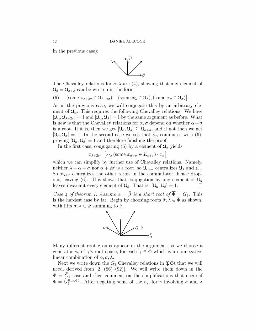
Case 4 of theorem 1. Assume α = β is a short root of Φ = G2. Thisis the hardest case by far. Begin by choosing roots σ, λ ∈ Φ as shown,with lifts σ, λ ∈ Φ summing to β.

σ α, β

λ

Many different root groups appear in the argument, so we choose agenerator eγ of γ’s root space, for each γ ∈ Φ which is a nonnegativelinear combination of α, σ, λ.

Next we write down the G2 Chevalley relations in PSt that we willneed, derived from [2, (86)–(92)]. We will write them down in the

Φ = G2 case and then comment on the simplifications that occur if

Φ = G 0 mod 32 . After negating some of the eγ, for γ involving σ and λ

PRESENTATION OF AFFINE KAC-MOODY GROUPS OVER RINGS 13

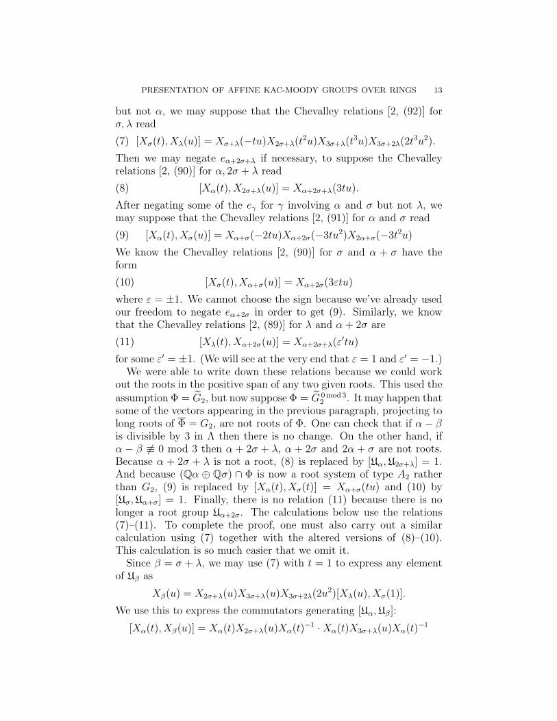
but not α, we may suppose that the Chevalley relations [2, (92)] forσ, λ read

(7) [Xσ(t), Xλ(u)] = Xσ+λ(−tu)X2σ+λ(t2u)X3σ+λ(t

3u)X3σ+2λ(2t3u2).

Then we may negate eα+2σ+λ if necessary, to suppose the Chevalleyrelations [2, (90)] for α, 2σ + λ read

(8) [Xα(t), X2σ+λ(u)] = Xα+2σ+λ(3tu).

After negating some of the eγ for γ involving α and σ but not λ, wemay suppose that the Chevalley relations [2, (91)] for α and σ read

(9) [Xα(t), Xσ(u)] = Xα+σ(−2tu)Xα+2σ(−3tu2)X2α+σ(−3t2u)

We know the Chevalley relations [2, (90)] for σ and α + σ have theform

(10) [Xσ(t), Xα+σ(u)] = Xα+2σ(3εtu)

where ε = ±1. We cannot choose the sign because we’ve already usedour freedom to negate eα+2σ in order to get (9). Similarly, we knowthat the Chevalley relations [2, (89)] for λ and α + 2σ are

(11) [Xλ(t), Xα+2σ(u)] = Xα+2σ+λ(ε′tu)

for some ε′ = ±1. (We will see at the very end that ε = 1 and ε′ = −1.)We were able to write down these relations because we could work

out the roots in the positive span of any two given roots. This used the

assumption Φ = G2, but now suppose Φ = G 0 mod 32 . It may happen that

some of the vectors appearing in the previous paragraph, projecting tolong roots of Φ = G2, are not roots of Φ. One can check that if α− βis divisible by 3 in Λ then there is no change. On the other hand, ifα − β 6≡ 0 mod 3 then α + 2σ + λ, α + 2σ and 2α + σ are not roots.Because α + 2σ + λ is not a root, (8) is replaced by [Uα,U2σ+λ] = 1.And because (Qα ⊕ Qσ) ∩ Φ is now a root system of type A2 ratherthan G2, (9) is replaced by [Xα(t), Xσ(t)] = Xα+σ(tu) and (10) by[Uσ,Uα+σ] = 1. Finally, there is no relation (11) because there is nolonger a root group Uα+2σ. The calculations below use the relations(7)–(11). To complete the proof, one must also carry out a similarcalculation using (7) together with the altered versions of (8)–(10).This calculation is so much easier that we omit it.

Since β = σ + λ, we may use (7) with t = 1 to express any elementof Uβ as

Xβ(u) = X2σ+λ(u)X3σ+λ(u)X3σ+2λ(2u2)[Xλ(u), Xσ(1)].

We use this to express the commutators generating [Uα,Uβ]:

[Xα(t), Xβ(u)] = Xα(t)X2σ+λ(u)Xα(t)−1 ·Xα(t)X3σ+λ(u)Xα(t)−1

14 DANIEL ALLCOCK

·Xα(t)X3σ+2λ(2u2)Xα(t)−1

·[Xα(t)Xλ(u)Xα(t)−1, Xα(t)Xσ(1)Xα(t)−1

]· [Xσ(1), Xλ(u)]

·X3σ+2λ(−2u2)X3σ+λ(−u)X2σ+λ(−u).

By (8) we may rewrite the first term (i.e., before the first dot) asXα+2σ+λ(3tu)X2σ+λ(u). By the Chevalley relations [Uα,U3σ+λ] = 1 wemay cancel the Xα(t)±1 in the second term. And similarly in the thirdterm, and in the first term of the first commutator. Then we rewritethe second term of that commutator using the Chevalley relations (9).The result is

[Xα(t), Xβ(u)] = Xα+2σ+λ(3tu)X2σ+λ(u)X3σ+λ(u)X3σ+2λ(2u2)

·[Xλ(u), Xα+σ(−2t)Xα+2σ(−3t)X2α+σ(−3t2)Xσ(1)

]·[Xσ(1), Xλ(u)

]·X3σ+2λ(−2u2)X3σ+λ(−u)X2σ+λ(−u).

(12)

Our next goal is the rewrite the first commutator [· · · , · · · ] on theright side. The first simplification is that all terms appearing in itcentralize U2α+σ. So we may drop the X2α+σ(−3t2) term. Then weexpand the commutator:

[· · · , · · · ] = Xλ(u)Xα+σ(−2t)Xα+2σ(−3t)Xσ(1)

·Xλ(−u)Xσ(−1)Xα+2σ(3t)Xα+σ(2t).

We will gather the Xλ and Xσ terms at the right end by repeated useof the Chevalley relations in PSt. We move Xσ(−1) across Xα+2σ(3t)using [Uσ,Uα+2σ] = 1. Then we move it across Xα+σ(2t) using thespecial case

Xσ(−1)Xα+σ(2t) = Xα+2σ(−6εt)Xα+σ(2t)Xσ(−1)

of (10). The result is

[· · · , · · · ] = Xλ(u)Xα+σ(−2t)Xα+2σ(−3t)Xσ(1)

·Xλ(−u)Xα+2σ(3t− 6εt)Xα+σ(2t)Xσ(−1).

Now we move Xλ(−u) across Xα+2σ(3t− 6εt) using the special case

Xλ(−u)Xα+2σ(3t− 6εt) = Xα+2σ+λ

(−3ε′tu(1− 2ε)

)·Xα+2σ(3t− 6εt)Xλ(−u)

of (11). Then we move it further right using [Uλ,Uα+σ] = 1:

[· · · , · · · ] = Xλ(u)Xα+σ(−2t)Xα+2σ(−3t)Xσ(1)

·Xα+2σ+λ

(−3ε′tu(1− 2ε)

)Xα+2σ(3t− 6εt)Xα+σ(2t)

PRESENTATION OF AFFINE KAC-MOODY GROUPS OVER RINGS 15

·Xλ(−u)Xσ(−1).

Now, Xσ(1) commutes with the two terms following it, and we appealto (10) to move it across Xα+σ(2t):

[· · · , · · · ] = Xλ(u)Xα+σ(−2t)Xα+2σ(−3t)Xα+2σ+λ

(−3ε′tu(1− 2ε)

)·Xα+2σ(3t)Xα+σ(2t)Xσ(1)Xλ(−u)Xσ(−1).

The second through fifth terms commute with each other, leading tomuch cancellation:

[· · · , · · · ] = Xλ(u)Xα+2σ+λ

(−3ε′tu(1− 2ε)

)Xσ(1)Xλ(−u)Xσ(−1).

Since Xλ(u) commutes with the term following it, we may rewrite thisas

[· · · , · · · ] = Xα+2σ+λ

(−3ε′tu(1− 2ε)

)[Xλ(u), Xσ(1)].

We plug this into (12) and cancel the commutators to get

[Xα(t), Xβ(u)] = Xα+2σ+λ(3tu)X2σ+λ(u)X3σ+λ(u)X3σ+2λ(2u2)

·Xα+2σ+λ

(−3ε′tu(1− 2ε)

)X3σ+2λ(−2u2)

·X3σ+λ(−u)X2σ+λ(−u).

Now, α+ 2σ+λ and 3σ+ 2λ are distinct roots, both projecting to thesame long root of Φ. In case 1 we established the Chevalley relations inPSt for two such roots, so the Xα+2σ+λ term in the middle commuteswith the X3σ+2λ term that precedes it. It centralizes the two termsbefore that by the Chevalley relations in PSt. So all the terms on theright cancel except the Xα+2σ+λ terms, leaving

[Xα(t), Xβ(u)] = Xα+2σ+λ

(3tu(1− ε′ + 2εε′)

)= Xα+2σ+λ(Ctu)

where C = 0, ±6 or 12 depending on ε, ε′ ∈ {±1}.If C = 0 (i.e., ε = 1 and ε′ = −1) then we have established the

desired Chevalley relation [Uα,Uβ] = 1 and the proof is complete. Oth-erwise we pass to the quotient St of PSt. Here Uα and Uβ commute,so we derive the relation Xα+2σ+λ(12t) = 1 in St. Since this identityholds universally, it holds for R = C, so the image of Uα+2σ+λ(C) inSt(C) is the trivial group. This is a contradiction, since St(C) actson the Kac-Moody algebra g, with Xα+2σ+λ(t) acting (nontrivially fort 6= 0) by exp ad(teα+2σ+λ). Since C 6= 0 leads to a contradiction, wemust have C = 0 and so the Chevalley relation [Uα,Uβ] = 1 holds inPSt. �

16 DANIEL ALLCOCK

Case 5 of theorem 1. Assume β = 2α in Φ = BCn≥2. Choose µ, λ ∈ Φas shown, and lift them to µ, λ ∈ Φ with µ + λ = β. (Mnemonic: µ ismiddling and λ is long.)

λα

β

µ

As in the case 2 (when α and β were the same long root of Φ = Bn),we can express any element of Uβ in the form[

(some xλ ∈ Uλ), (some xµ ∈ Uµ)]· (some xµ+λ ∈ Uµ+λ).

Among the Chevalley relations in PSt is the commutativity of Uα withUλ, Uµ and Uµ+λ. So Uα also centralizes Uβ. �

Case 6 of theorem 1. Assume α = β is a short root of Φ = BCn≥2

and α + β is a root. This is the exceptional case of lemma 5, andthe Chevalley relation we must establish is not [Uα,Uβ] = 1. We willdetermine the correct relation during the proof. We begin by choosingµ, σ ∈ Φ as shown and lifting them to µ, σ ∈ Φ with µ+ σ = β, so σ, µgenerate a B2 root system.

σ α, βµ

We choose a generator eγ for the root space of each nonnegative linearcombination γ ∈ Φ of α, σ, µ. By changing the signs of eσ+µ and e2σ+µ

if necessary, we may suppose that the Chevalley relations [2, (85)] forσ, µ are

(13) [Xσ(t), Xµ(u)] = Xσ+µ(−tu)X2σ+µ(t2u),

Since σ + µ = β we may take t = 1 in (13) to express any element ofUβ:

(14) Xβ(u) = X2σ+µ(u)[Xµ(u), Xσ(1)].

Using this one can express any generator for [Uα,Uβ]:

[Xα(t), Xβ(u)] = Xα(t)X2σ+µ(u)Xα(t)−1

·[Xα(t)Xµ(u)Xα(t)−1, Xα(t)Xσ(1)Xα(t)−1

]· [Xσ(1), Xµ(u)] ·X2σ+µ(−u).

(15)

By the Chevalley relations [Uα,U2σ+µ] = [Uα,Uµ] = 1, the Xα(t)±1’scancel in the first term and in the first term of the first commutator.

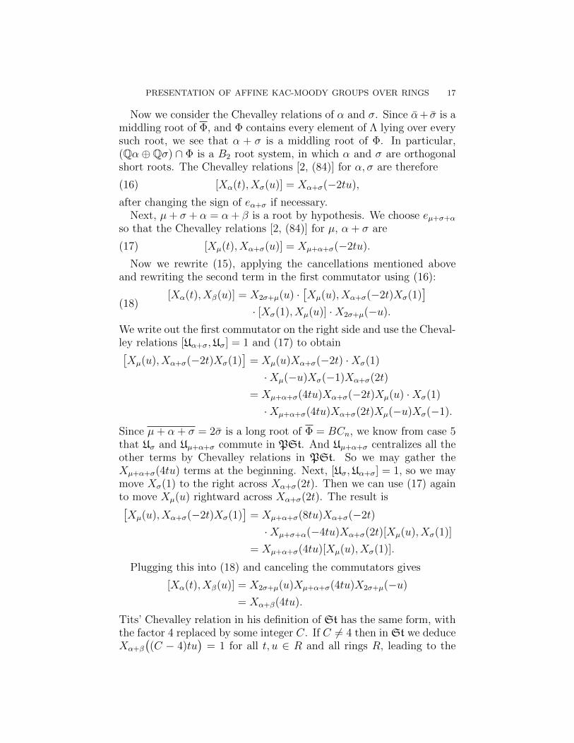
PRESENTATION OF AFFINE KAC-MOODY GROUPS OVER RINGS 17

Now we consider the Chevalley relations of α and σ. Since α+ σ is amiddling root of Φ, and Φ contains every element of Λ lying over everysuch root, we see that α + σ is a middling root of Φ. In particular,(Qα ⊕ Qσ) ∩ Φ is a B2 root system, in which α and σ are orthogonalshort roots. The Chevalley relations [2, (84)] for α, σ are therefore

(16) [Xα(t), Xσ(u)] = Xα+σ(−2tu),

after changing the sign of eα+σ if necessary.Next, µ+ σ + α = α+ β is a root by hypothesis. We choose eµ+σ+α

so that the Chevalley relations [2, (84)] for µ, α + σ are

(17) [Xµ(t), Xα+σ(u)] = Xµ+α+σ(−2tu).

Now we rewrite (15), applying the cancellations mentioned aboveand rewriting the second term in the first commutator using (16):

[Xα(t), Xβ(u)] = X2σ+µ(u) ·[Xµ(u), Xα+σ(−2t)Xσ(1)

]· [Xσ(1), Xµ(u)] ·X2σ+µ(−u).

(18)

We write out the first commutator on the right side and use the Cheval-ley relations [Uα+σ,Uσ] = 1 and (17) to obtain[Xµ(u), Xα+σ(−2t)Xσ(1)

]= Xµ(u)Xα+σ(−2t) ·Xσ(1)

·Xµ(−u)Xσ(−1)Xα+σ(2t)

= Xµ+α+σ(4tu)Xα+σ(−2t)Xµ(u) ·Xσ(1)

·Xµ+α+σ(4tu)Xα+σ(2t)Xµ(−u)Xσ(−1).

Since µ+ α + σ = 2σ is a long root of Φ = BCn, we know from case 5that Uσ and Uµ+α+σ commute in PSt. And Uµ+α+σ centralizes all theother terms by Chevalley relations in PSt. So we may gather theXµ+α+σ(4tu) terms at the beginning. Next, [Uσ,Uα+σ] = 1, so we maymove Xσ(1) to the right across Xα+σ(2t). Then we can use (17) againto move Xµ(u) rightward across Xα+σ(2t). The result is[Xµ(u), Xα+σ(−2t)Xσ(1)

]= Xµ+α+σ(8tu)Xα+σ(−2t)

·Xµ+σ+α(−4tu)Xα+σ(2t)[Xµ(u), Xσ(1)]

= Xµ+α+σ(4tu)[Xµ(u), Xσ(1)].

Plugging this into (18) and canceling the commutators gives

[Xα(t), Xβ(u)] = X2σ+µ(u)Xµ+α+σ(4tu)X2σ+µ(−u)

= Xα+β(4tu).

Tits’ Chevalley relation in his definition of St has the same form, withthe factor 4 replaced by some integer C. If C 6= 4 then in St we deduceXα+β

((C − 4)tu

)= 1 for all t, u ∈ R and all rings R, leading to the

18 DANIEL ALLCOCK

same contradiction we found in case 4. Therefore C = 4 and we haveestablished that Tits’ relation already holds in PSt. �

Case 7 of theorem 1. Assume α = β is a short root of Φ = BCn≥2

and α + β is not a root. This is similar to the previous case butmuch easier. We choose µ, σ and the eγ in the same way, except thatµ+σ+α is no longer a root, so the Chevalley relation (17) is replacedby [Uµ,Uα+σ] = 1. We expand Xβ(u) as in (14) and obtain (18) asbefore. But this time the Xα+σ(−2t) term centralizes both Uµ andUσ, so it vanishes from the commutator. The right side of (18) thencollapses to 1 and we have proven [Uα,Uβ] = 1 in PSt. �

5. Finite presentations

In this section we prove theorem 3, that various Steinberg and Kac-Moody groups are finitely presented. At the end we make several re-marks about possible variations on the definition of Kac-Moody groups.

Proof of theorem 3. We must show that StA(R) is finitely presentedunder either of the two stated hypotheses. By theorem 1 it suffices toprove this with PSt in place of St.

(ii) We are assuming rkA ≥ 3 and that R is finitely generatedas a module over a subring generated by finitely many units. The-orem 1.4(ii) of [2] shows that if R satisfies this hypothesis and A is2-spherical, then PStA(R) is finitely presented. This proves (ii).

(i) Now we are assuming rkA > 3 and that R is finitely generated asa ring. Theorem 1.4(iii) of [2] gives the finite presentability of PStA(R)if every pair of nodes of the Dynkin diagram lies in some irreduciblespherical diagram of rank ≥ 3. By inspecting the list of affine Dynkindiagrams of rank > 3, one checks that this treats all cases of (i) except

A =α β γ δ

(with some orientations of the double edges). In this case, no irre-ducible spherical diagram contains α and δ.

For this case we use a variation on the proof of theorem 1.4(iii) of [2].Consider the direct limit G of the groups StB(R) as B varies over allirreducible spherical diagrams of rank ≥ 2. If rkB ≥ 3 then StB(R)is finitely presented by theorem I of Splitthoff [17]. If rkB = 2 thenStB(R) is finitely generated by [2, thm. 11.5]. Since every irreduciblerank 2 diagram lies in one of rank > 2, it follows that G is finitelypresented. Now, G satisfies all the relations of StA(R) except for thecommutativity of St{α} with St{δ}. Because these groups may not be

PRESENTATION OF AFFINE KAC-MOODY GROUPS OVER RINGS 19

finitely generated, we might need infinitely many additional relationsto impose commutativity in the obvious way.

So we proceed indirectly. Let Yα be a finite subset of St{α} whichtogether with St{β} generates St{α,β}. This is possible since St{α,β}is finitely generated. We define Yδ similarly, with γ in place of β. Wedefine H as the quotient of G by the finitely many relations [Yα, Yδ] = 1,and claim that the images in H of St{α} and St{δ} commute.

The following computation in H establishes this. First, every ele-ment of Yδ centralizes St{β} by the definition of G, and every elementof Yα by definition of H. Therefore it centralizes St{α,β}, hence St{α}.We’ve shown that St{α} centralizes Yδ, and it centralizes St{γ} by thedefinition of G. Therefore it centralizes St{γ,δ}, hence St{δ}.H has the same generators as PStA(R), and its defining relations are

among those defining PStA(R). On the other hand, we have shownthat the generators of H satisfy all the relations in PStA(R). SoH ∼= PStA(R). In particular, PStA(R) is finitely presented.

It remains to prove the finite presentability of GA(R) under the extrahypothesis that the unit group of R is finitely generated as an abeliangroup. This follows immediately from [2, Lemma 11.2], which says thatfor any generalized Cartan matrix A, and any commutative ring R withfinitely generated unit group, the kernel of StA(R)→ GA(R) is finitelygenerated. �

Remark (Completions). We have worked with the “minimal” or “alge-braic” forms of Kac-Moody groups. One can consider various comple-tions of it, such as those surveyed in [19]. None of these completionscan possibly be finitely presented, so no analogue of theorem 3 exists.But it is reasonable to hope for an analogue of corollary 2.

Remark (Chevalley-Demazure group schemes). If A is spherical thenwe write CDA for the associated Chevalley-Demazure group scheme,say the simply-connected version. This is the unique most natural (ina certain technical sense) algebraic group over Z of type A. The kernelof StA(R)→ CDA(R) is called K2(A;R) and contains the relators (1).There is considerable interest in when CDA(R) is finitely presented, forexample [5][6]. We want to emphasize that our theorem 3 does notresolve this question, because CDA(R) may be a proper quotient ofGA(R). Indeed, K2(A;R) can be extremely complicated.

For a non-spherical Dynkin diagram A, the functor CDA is not de-fined. The question of whether there is a good definition, and whatit would be, seems to be completely open. Only when R is a field isthere known to be a unique “best” definition of a Kac-Moody group[20, theorem 1(i), p. 553]. The main problem would be to specify what

20 DANIEL ALLCOCK

extra relations to impose on GA(R). The remarks below discuss thepossible forms of some additional relations.

Remark (Kac-Moody groups over integral domains). If R is an integraldomain with fraction field k, then it is open whether GA(R) → GA(k)is injective. If GA satisfies Tits’ axioms then this would follow from(KMG4), but Tits does not assert that GA satisfies his axioms. IfGA(R) → GA(k) is not injective, then the image seems better thanGA(R) itself as a candidate for the right Kac-Moody group.

Remark (Kac-Moody groups via representations). Fix a root datum Dand a commutative ring R. By using Kostant’s Z-form of the universalenveloping algebra of g, one can construct a Z-form V λ

Z of any integrablehighest-weight module V λ of g. Then one defines V λ

R as V λZ ⊗ R. For

each real root α, one can exponentiate gα,Z⊗R ∼= R to get an action ofUα ∼= R on V λ

R . One can define the action of the torus (R∗)n directly.Then one can take the group Gλ

D(R) generated by these transformationsand call it a Kac-Moody group. This approach is extremely natural andnot yet fully worked out. The first such work for Kac-Moody groupsover rings is Garland’s landmark paper [11] treating affine groups; seealso Tits’ survey [19, §5], its references, and the recent articles [4][7].

Tits [20, p. 554] asserts that this construction allows one to builda Kac-Moody functor satisfying all his axioms (KMG1)–(KMG9). Weimagine that he reasoned as follows. First, show that each Gλ

D is aKac-Moody functor and therefore by Tits’ theorem admits a canonicalfunctorial homomorphism from GA, where A is the generalized Cartanmatrix of D. (One cannot directly apply Tits’ theorem, because Gλ

D(R)only comes equipped with the homomorphisms SL2(R) → Gλ

D(R) re-quired by Tits when SL2(R) is generated by its subgroups

(1 ∗0 1

)and(

1 0∗ 1

). Presumably this difficulty can be overcome.) Second, define I

as the intersection of the kernels of all the homomorphisms GA → GλD,

and then define the desired Kac-Moody functor as GA/I. (This alsodoes not quite make sense, since GA may also lack the required ho-momorphisms from SL2. As before, presumably this difficulty can beovercome.)

Remark (Loop groups). SupposeX is one of the ABCDEFG diagrams,

X is its affine extension as in section 4, and R is a commutative ring.The well-known description of affine Kac-Moody algebras and loopgroups makes it natural to expect that GX(R) is a central extensionof GX(R[t±1]) by R∗. The most general results along these lines thatI know of are Garland’s theorems 10.1 and B.1 in [11], although theyconcern slightly different groups. Instead, one might simply define the

PRESENTATION OF AFFINE KAC-MOODY GROUPS OVER RINGS 21

loop group GX(R) as a central extension of CDX(R[t±1]) by R∗, wherethe 2-cocycle defining the extension would have to be made explicit.Then one could try to show that GX satisfies Tits’ axioms.

It is natural to ask whether such a group GX(R) would be finitelypresented if R is finitely generated. If R∗ is finitely generated then thisis equivalent to the finite presentation of the quotient CDX(R[t±1]). IfrkX ≥ 3 then StX(R[t±1]) is finitely presented by Splitthoff’s theo-rem I of [17]. Then, as Splitthoff explains in [17, §7], the finite pre-sentability of CDX(R[t±1]) boils down to properties of K1(X,R[t±1])and K2(X,R[t±1]).

References

[1] Abramenko, P. and Muhlherr, B., Presentations de certaines BN -pairesjumelees comme sommes amalgamees, C.R.A.S. Serie I 325 (1997) 701–706.

[2] Allcock, Steinberg groups as amalgams, preprint arXiv:1307.2689v2.[3] Allcock, D. and Carbone, L., Presentation of hyperbolic Kac-Moody groups

over rings, preprint arXiv:1409.5918.[4] Bao, L. and Carbone, L., Integral forms of Kac-Moody groups and Eisenstein

series in low dimensional supergravity theories, arXiv:1308.6194v1.[5] Behr, H., Uber die endliche Definierbarkeit verallgemeinerter Einheitsgruppen

II, Invent. Math. 4 (1967) 265–274.[6] Behr, H., Arithmetic groups over function fields I, J. reine angew. Math. bf

495 (1998) 79–118.[7] Carbone, L. and Garland, H., Infinite dimensional Chevalley groups and Kac-

Moody groups over Z, in preparation (2013).[8] Caprace, P.-E., On 2-spherical Kac-Moody groups and their central extensions,

Forum Math. 19 (2007) 763–781.[9] Eskin, A., and Farb, B., Quasi-flats and rigidity in higher rank symmetric

spaces, J.A.M.S. 10 (1997) 653–692.[10] Farb, B. and Schwartz, R., The large-scale geometry of Hilbert modular groups,

J. Diff. Geom. 44 (1996) 435–478.[11] Garland, H. The arithmetic theory of loop groups, Publ. Math. I.H.E.S. 52

(1980) 5–136.[12] Kac, V., Infinite dimensional Lie algebras (3rd edition), Cambridge University

Press, Cambridge, 1990.[13] Kleiner, B. and Leeb, B., Rigidity of quasi-isometries for symmetric spaces and

Euclidean buildings, Publ. math. I.H.E.S. 86 (1997) 115–197.[14] Morita, J. and Rehmann, U., A Matusumoto-type theorem for Kac-Moody

groups, Tohoku Math. J. 42 (1990) 537–560.[15] Muhlherr, B., On the simple connectedness of a chamber system associated to

a twin building, unpublished (1999).[16] Schwartz, R., The quasi-isometry classification of rank one lattices, Publ. Math.

I.H.E.S. 82 (1995) 133–168.[17] Splitthoff, S., Finite presentability of Steinberg groups and related Chevalley

groups. in Applications of algebraic K-theory to algebraic geometry and number

22 DANIEL ALLCOCK

theory, Part I, II (Boulder, Colo., 1983), pp. 635–687, Contemp. Math. 55,Amer. Math. Soc., Providence, RI, 1986.

[18] Steinberg, R., Lectures on Chevalley groups. Notes prepared by John Faulknerand Robert Wilson, Yale University, New Haven, Conn., 1968.

[19] Tits, J., Groups and group functors attached to Kac-Moody data, in WorkshopBonn 1984, pp. 193–223, Lecture Notes in Math. 1111, Springer, Berlin, 1985.

[20] Tits, J., Uniqueness and presentation of Kac-Moody groups over fields, J.Algebra 105 (1987) 542–573.

Department of Mathematics, University of Texas, AustinE-mail address: allcock@math.utexas.eduURL: http://www.math.utexas.edu/~allcock