Presentación de PowerPoint - Comprise · Poisson Reconstruction For the reconstruction, we convert...
133
Ciclop 3D Scanner
Transcript of Presentación de PowerPoint - Comprise · Poisson Reconstruction For the reconstruction, we convert...
Ciclop3D Scanner

What is Ciclop?
• First DIY 3D Scanner
• Fully customizable
• 30 minutes assembling
• Open-Source

• Scanning volume: 20 cm (diameter) x 20 cm (height)
• Accuracy around 0,5mm (according to calibration)• BQ ZUM BT-328 & ZUM Scan
• Ready to connect 2 motors, 4 lasers, or one LDR.
What is Ciclop?

Hardware: Easy to build and open to improve

The technology: Laser triangulation

Lasers impact on the rotating piece
The camera collects the surface information, analyzes and recreates the
figure
The technology: Laser triangulation

Auto-calibration: A differential value

Software: Open to the future
• Camera Drivers • Reconstruction
software• HORUS
Meshlab
CloudCompare
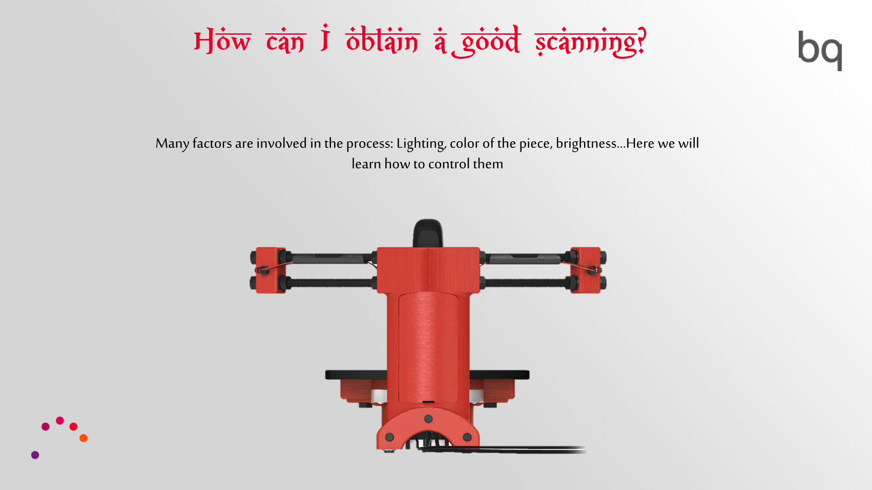
Many factors are involved in the process: Lighting, color of the piece, brightness…Here we will learn how to control them
How can I obtain a good scanning?

Ambient Lighting
Lighting should be uniform, indirect and medium intensity. Thus, the appearance of reflections and shadows are avoided.

A commendable idea is to set a direct light from the back, with some dispersion and not concentrated
Ambient Lighting

Object material
Objects with glossy finishes are difficult to scan because they can produce glare. But that does not mean it is not possible

The next piece is a metal screw. It may seems impossible to scan
Object material

But there is the possibility of applying a watercolor or acrylic paint water-soluble covering the piece and remove all metallic sheen, making it matte
Object material
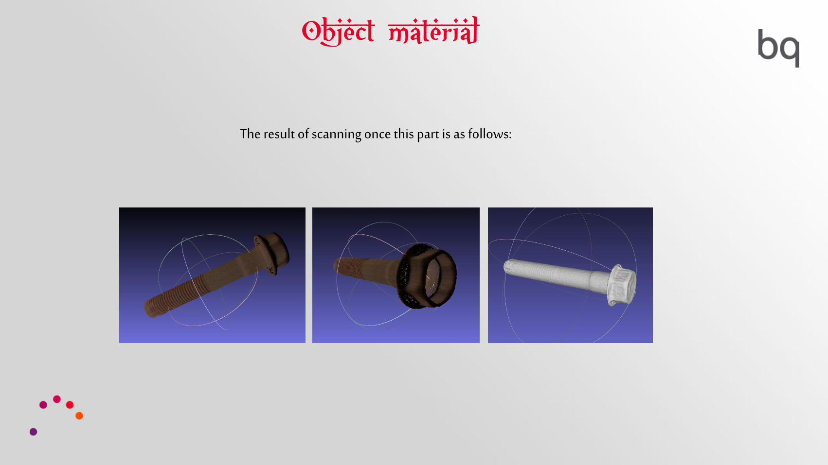
The result of scanning once this part is as follows:
Object material

A next step would be the possible re-design of the piece (applying a smoothing with a 3D software for example)
Object material

Another metallic example, which was painted and then scanned:
Object material

Object color
The laser beam is red, so that color objects can cause problems when it comes to recognition.

Object color
Light-colored objects can cause problems, especially in high brightness environments. In these cases it is recommended to decrease the brightness
Uncorrectedbrightness
Brightnessdiminished
Object color
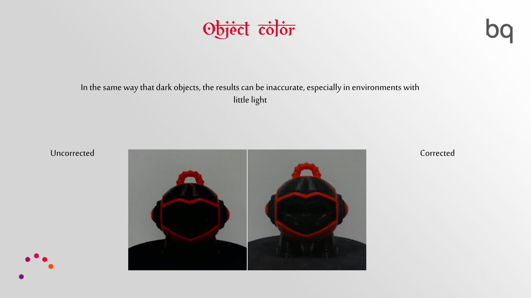
In the same way that dark objects, the results can be inaccurate, especially in environments with little light
Uncorrected Corrected

Object color
It is recommended to decrease the contrast and exposure increase a little, in addition to lowering the threshold
Uncorrected Corrected

Object color
The ideal would be a non- aggressive or very intense color, matte and dull
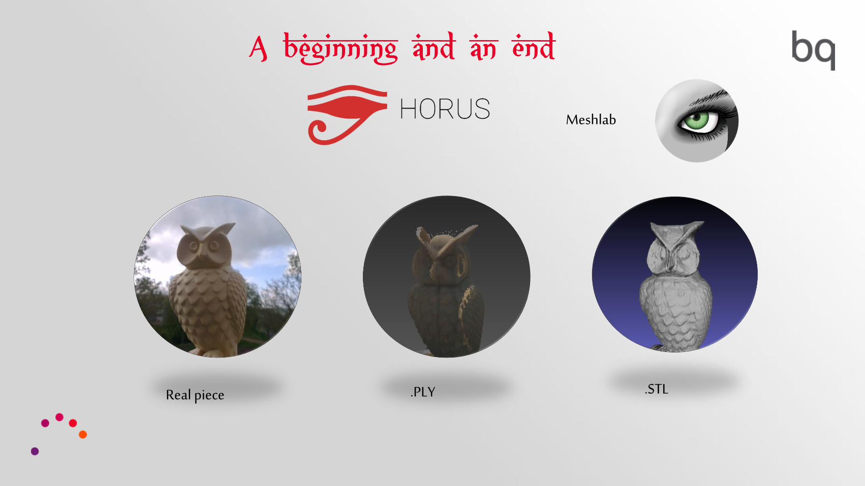
A beginning and an end
Meshlab
.PLY .STLReal piece

A beginning and an end
Meshlab
.PLY .STLReal piece
Calibration
Scanning
Reconstruction
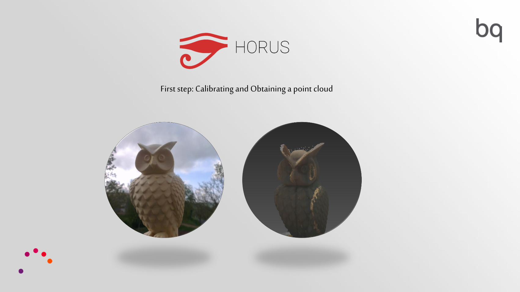
First step: Calibrating and Obtaining a point cloud

1. Wizard Mode 2. Control Workbench
3. CalibrationWorkbench
4. Scanning Workbench
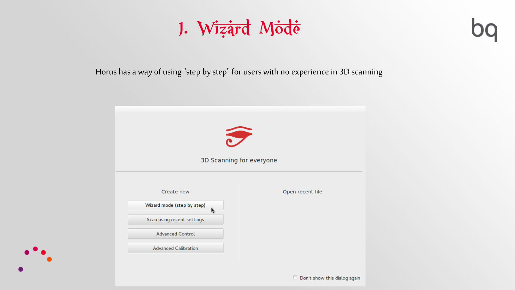
1. Wizard Mode
Horus has a way of using "step by step" for users with no experience in 3D scanning

1. Wizard Mode
It opens every time the program is started, or from the File menu

1. Wizard Mode
When you start the Wizard, this is the screen displayed
1. Wizard Mode
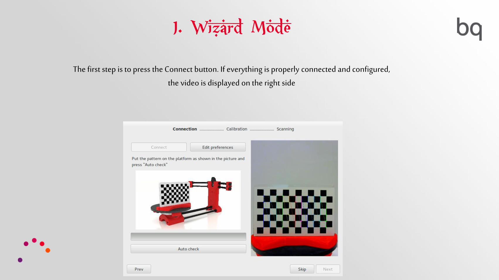
The first step is to press the Connect button. If everything is properly connected and configured,
the video is displayed on the right side
1. Wizard Mode
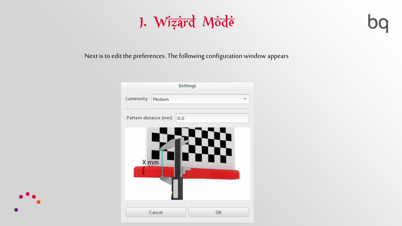
Next is to edit the preferences. The following configuration window appears

1. Wizard Mode
It may be modified brightness and distance of the pattern.

1. Wizard Mode
Pattern is the distance in mm, from the upper side of the square in the lower left part of the
pattern to the rotating platform of the scanner
1. Wizard Mode
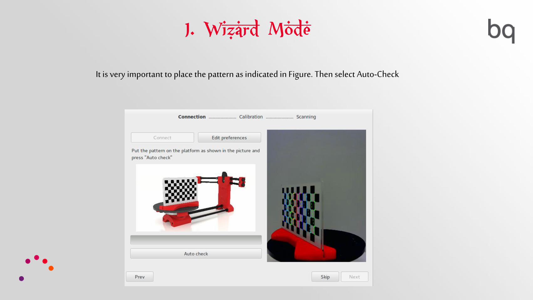
It is very important to place the pattern as indicated in Figure. Then select Auto-Check

1. Wizard Mode
If this is the first time the scanner is configured, the following window will appear. This dialogue
lasers recommend setting manually to get a vertical position.

1. Wizard Mode
If the button YES is pressed both lasers will light. Using the calibration pattern, lasers will be
placed vertically. To make this adjustment we will use the screws
1. Wizard Mode
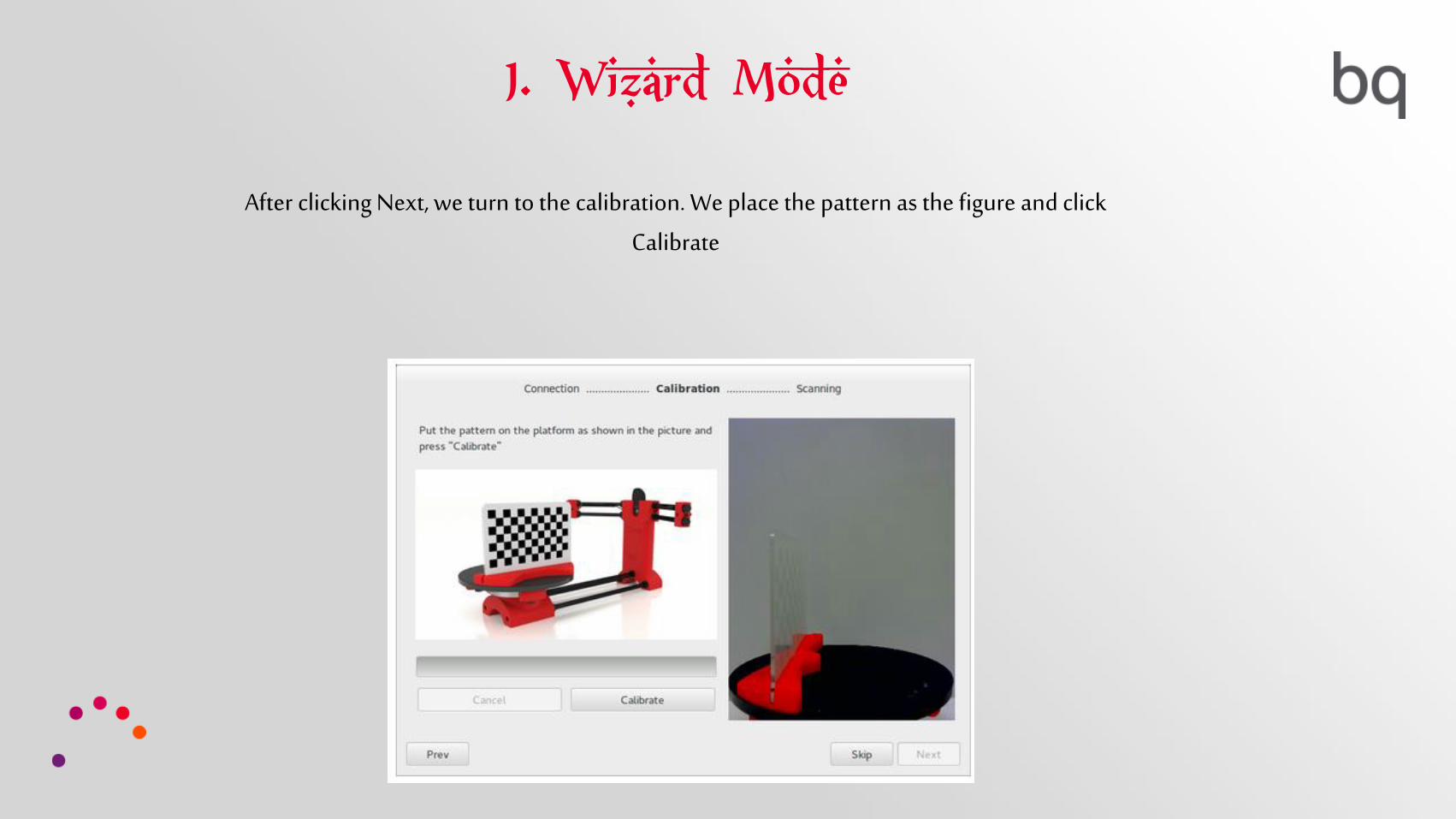
After clicking Next, we turn to the calibration. We place the pattern as the figure and click
Calibrate

1. Wizard Mode
After pressing Calibrate, start the process
1. Wizard Mode
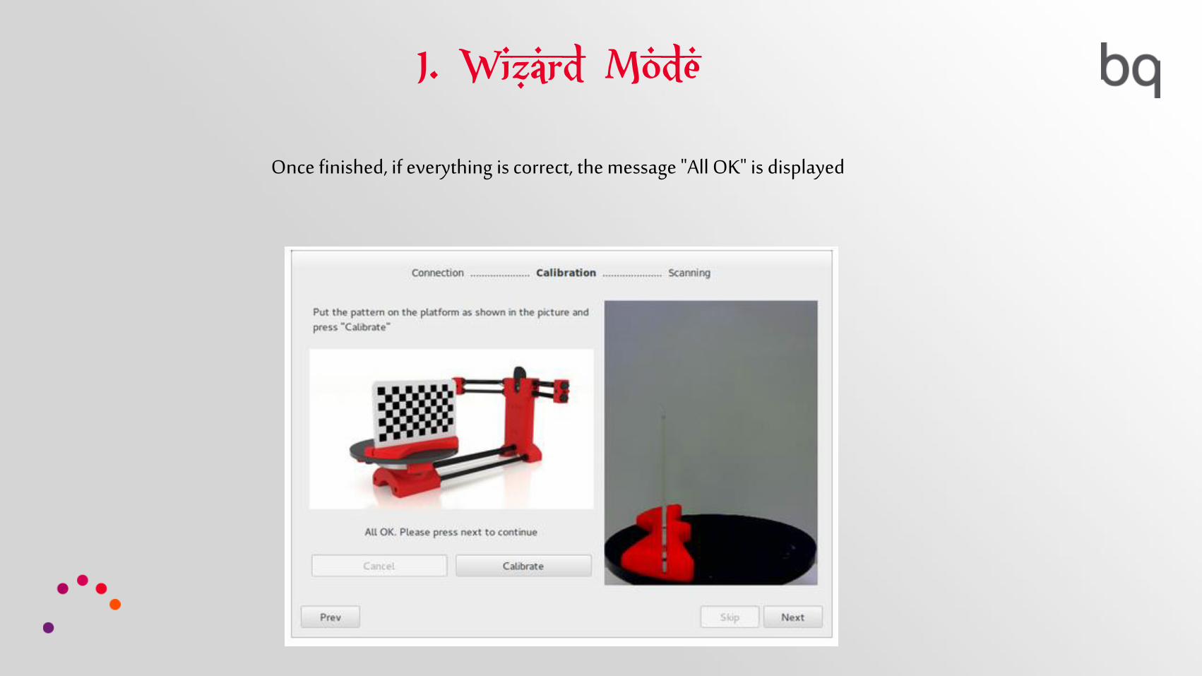
Once finished, if everything is correct, the message "All OK" is displayed
1. Wizard Mode
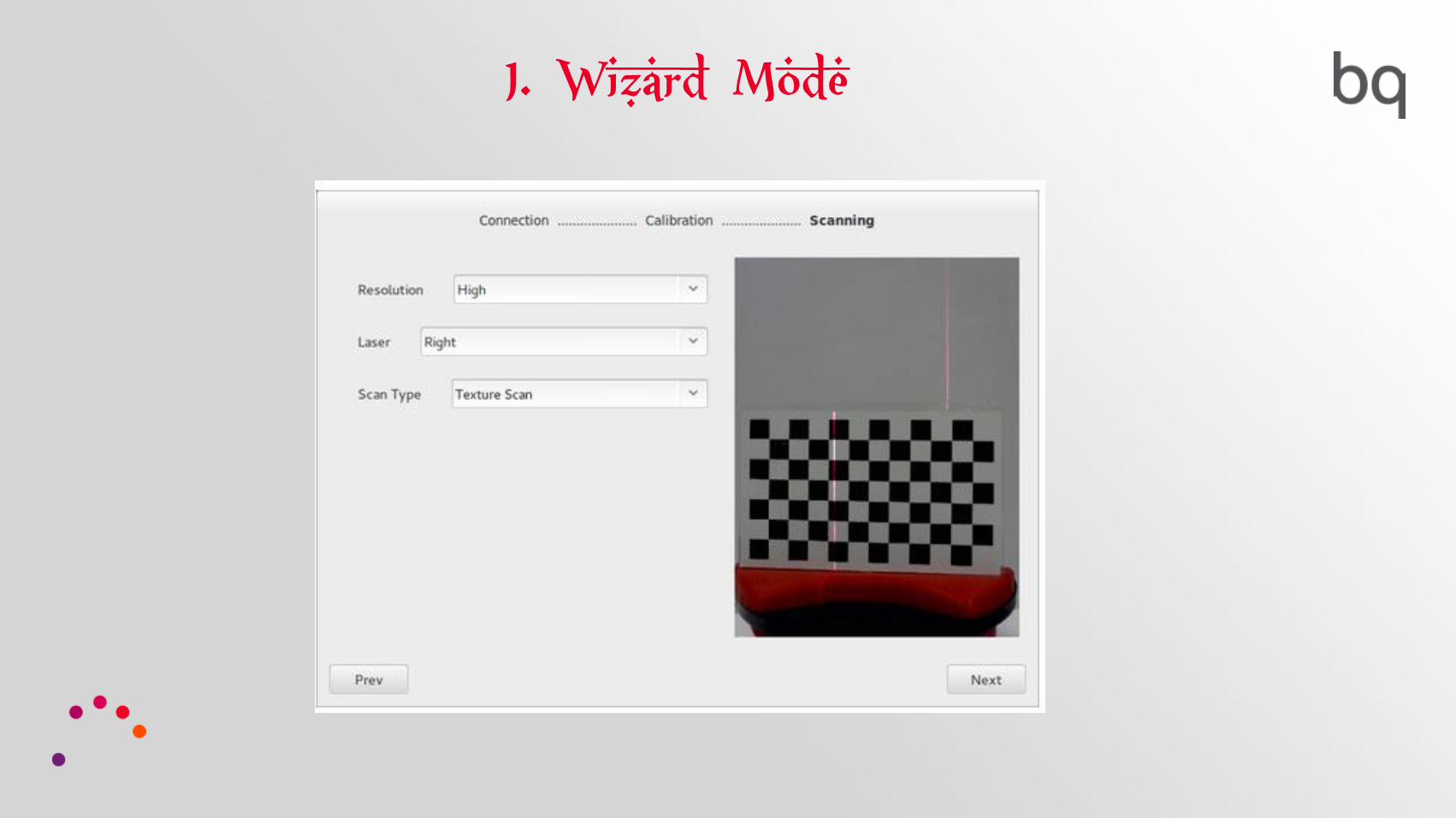
The last step of the Wizard will set the scan preferences. This screen shows the available options

1. Wizard Mode
Resolution: High resolution, Medium resolution, Low resolution. The higher it is, the higher the
scan time
1. Wizard Mode
Laser: It can be used the left laser, right laser, or both. If we use both, the amount of scanned
points will be higher, so our piece will be more detailed

1. Wizard Mode
Scanning Type: It can be used Simple scanning or With Texture. The simple scanning doesn’t
catch the object color. The scanning with texture uses 2 Images to catch the laser, generating the mesh of points with the real colors of the object
1. Wizard Mode

1. Wizard Mode
Once the Preference Scanning Settings are finished, we press Next, and the scanner will be
ready to start working
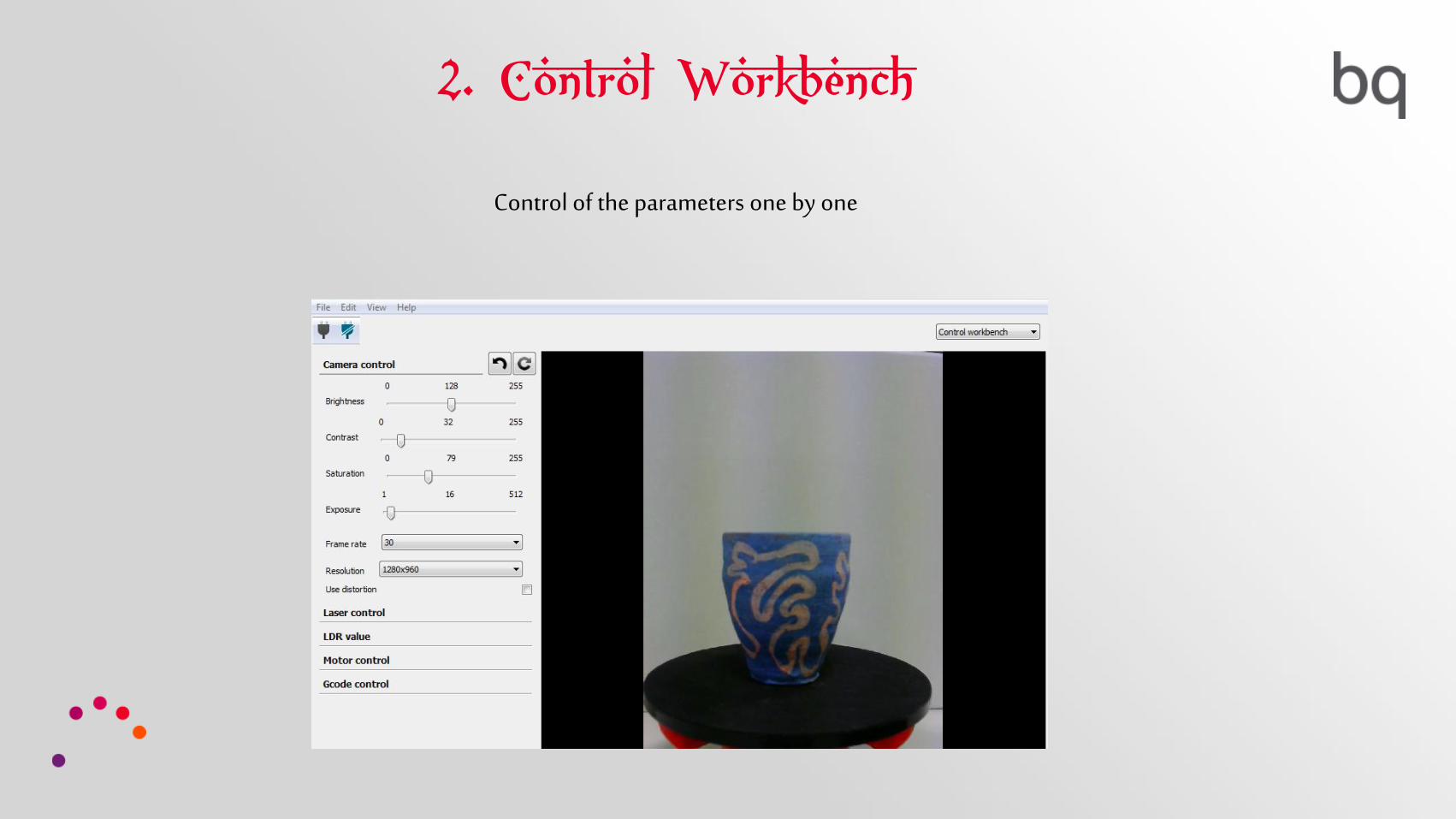
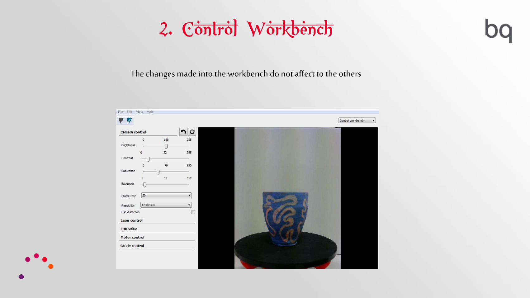
2. Control Workbench
Control of the parameters one by one
2. Control Workbench
The changes made into the workbench do not affect to the others

2. Control Workbench
Its goal is to experiment and learn about the different parameters
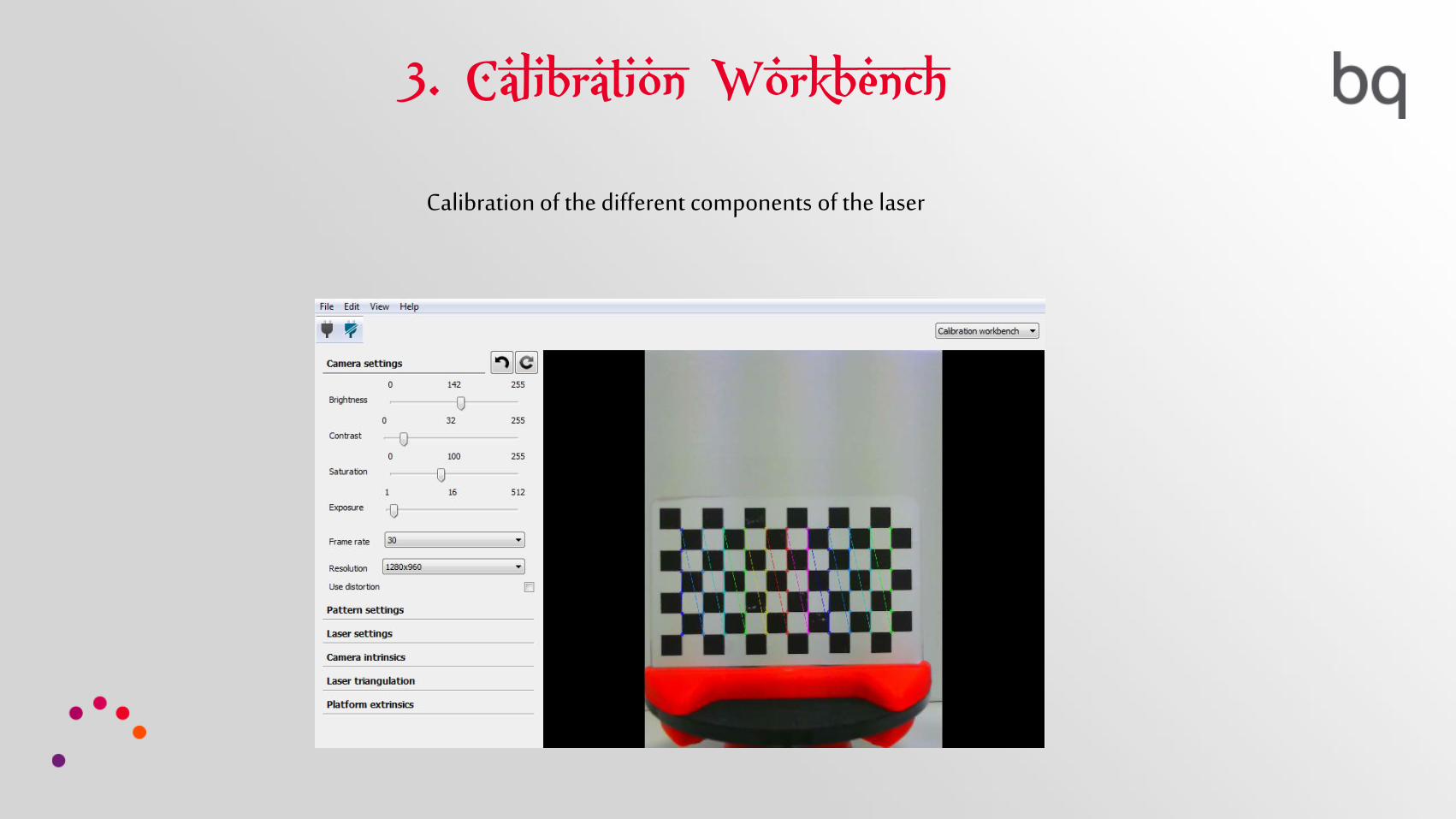
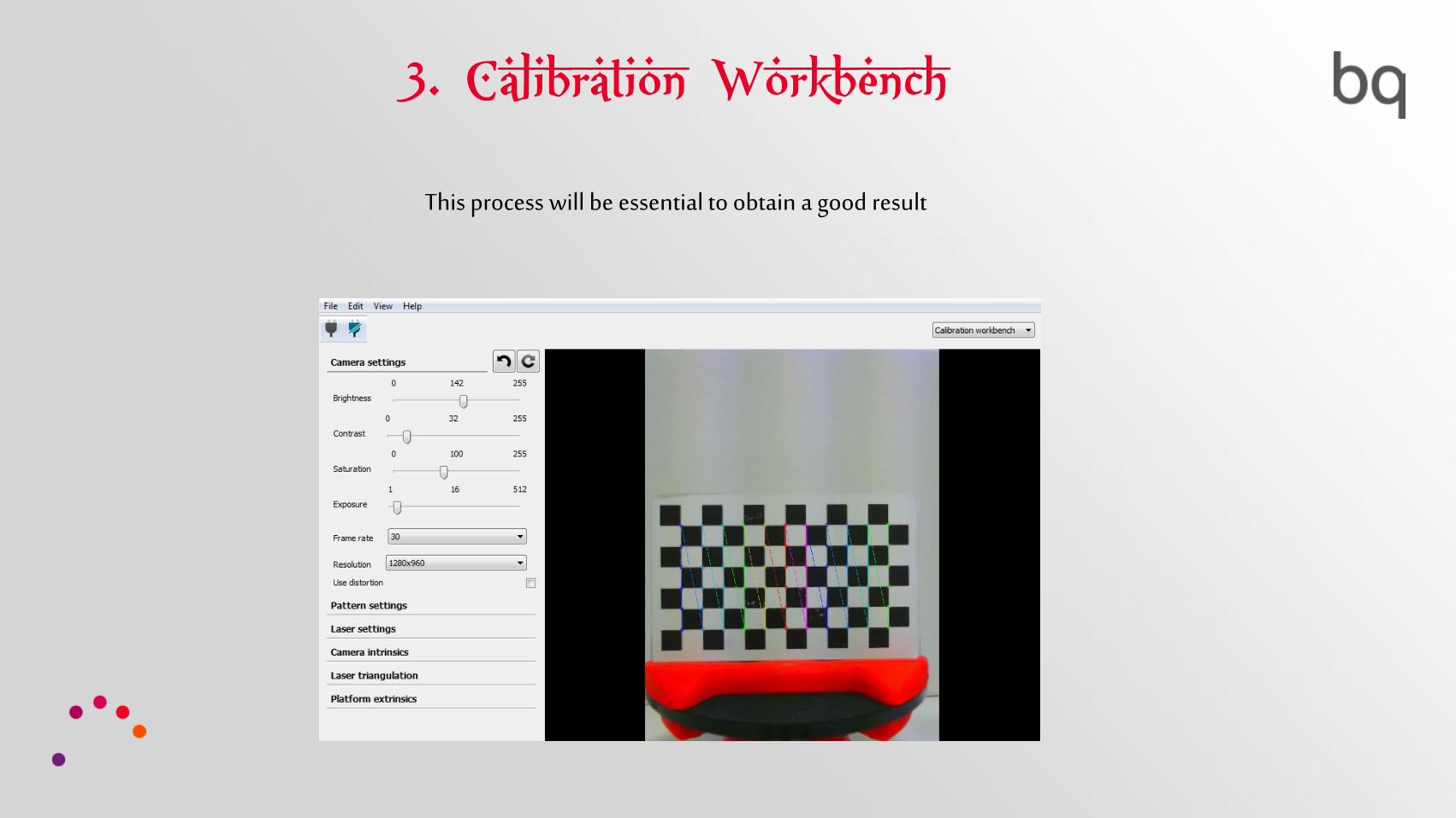
3. Calibration Workbench
Calibration of the different components of the laser

3. Calibration Workbench
The changes made into the workbench affect to the others
3. Calibration Workbench
This process will be essential to obtain a good result
3. Calibration Workbench
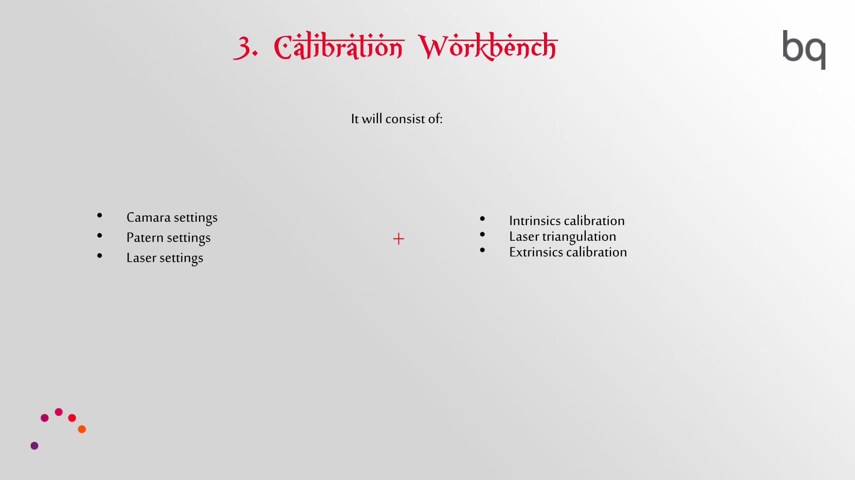
It will consist of:
• Camara settings• Patern settings• Laser settings
• Intrinsics calibration• Laser triangulation• Extrinsics calibration
+
3. Calibration Workbench
The camera settings aims to ensure that the pattern is detected correctly, in different positions
Camera Settingsand lighting conditions of the scene.
Camera Settings:
3. Calibration Workbench
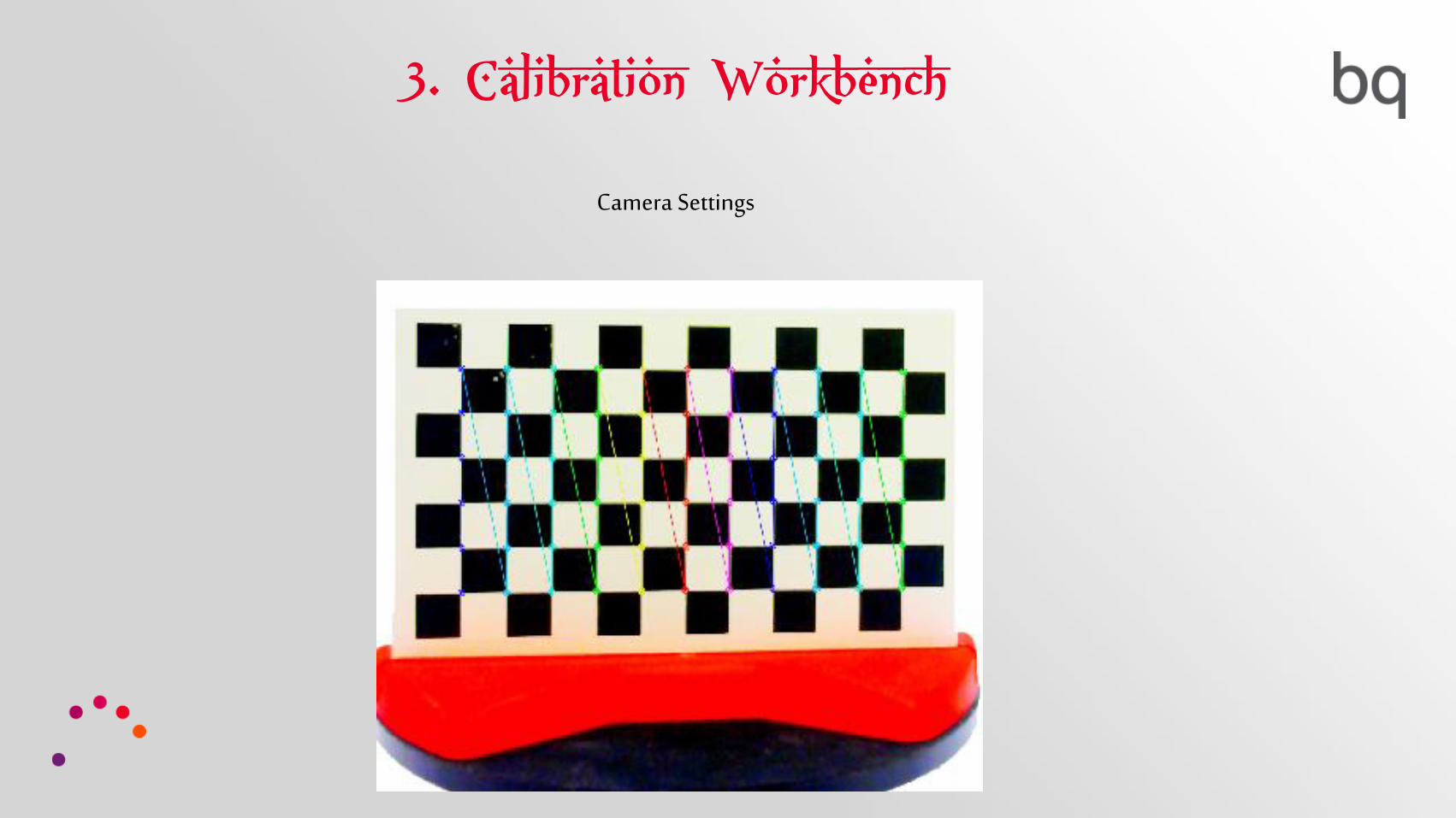
Camera Settings

3. Calibration Workbench
Camera Settings
Brightness: Brightness of the image
3. Calibration Workbench
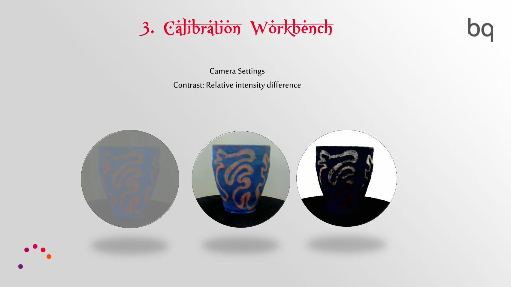
Camera Settings
Contrast: Relative intensity difference

3. Calibration Workbench
Camera Settings
Saturation: Intensity of color image

3. Calibration Workbench
Camera Settings
Exposure Time lens aperture (milliseconds)

3. Calibration Workbench
Camera Settings
Framerate: Images captured per second
Resolution: Image size. 4:3
Distortion: Distortion correction lens according to the calibration

3. Calibration Workbench
Patern Settings:
Calibration is done by a pattern
3. Calibration Workbench
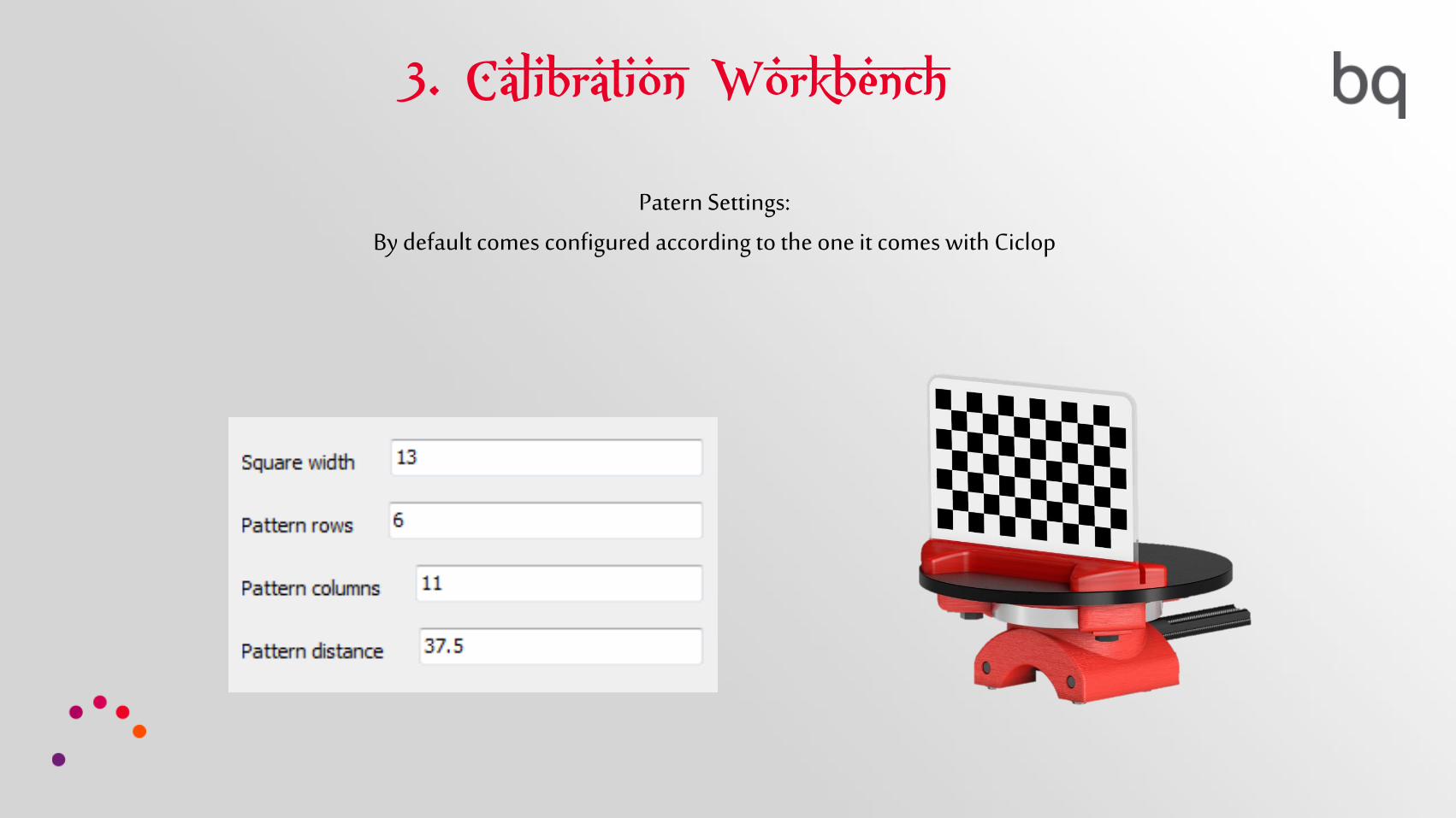
Patern Settings:
By default comes configured according to the one it comes with Ciclop

3. Calibration Workbench
Patern Settings:
The distance set will be the one shown in Figure

3. Calibration Workbench
Laser Settings:
Option Enable / Disable right, left Laser, or both

3. Calibration Workbench
Laser Settings:
They should be adjusted to be completely vertical relative to the platform

3. Calibration Workbench
Intrinsics Calibration:
The aim is to calculate:
• Focal lengths• Optical center• Lens distorsion
3. Calibration Workbench
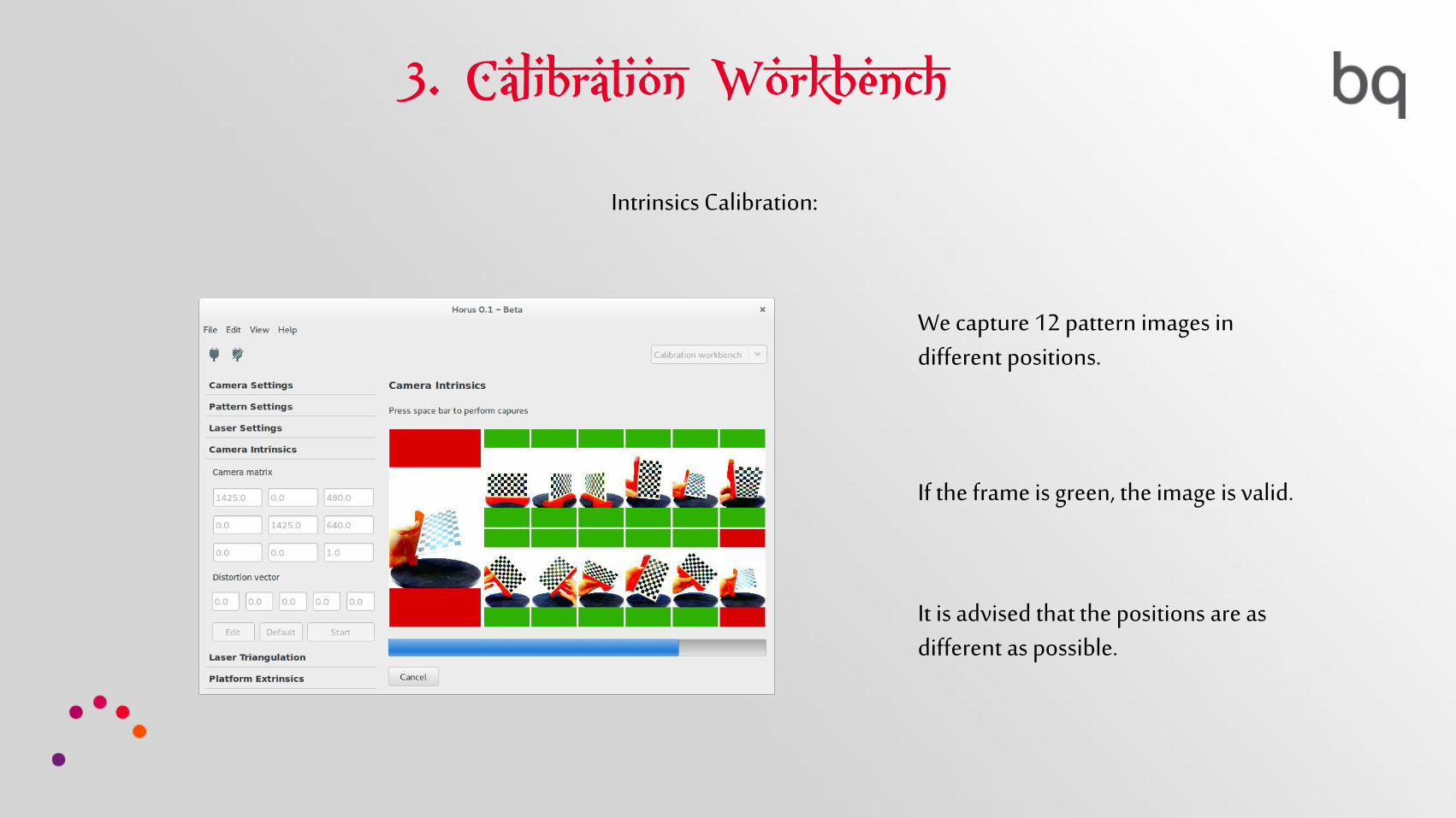
Intrinsics Calibration:
We capture 12 pattern images in different positions.
If the frame is green, the image is valid.
It is advised that the positions are as different as possible.

3. Calibration Workbench
Intrinsics Calibration:
The result is displayed numerically and graphically.
At this point, we can accept or reject the calibration.

3. Calibration Workbench
Laser Triangulation:
The aim is to calculate:
• Lasers tilt and distance from the camera to its intersection
3. Calibration Workbench
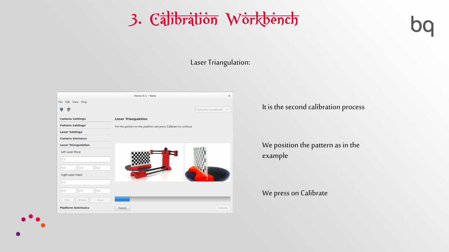
Laser Triangulation:
We position the pattern as in the example
We press on Calibrate
It is the second calibration process
3. Calibration Workbench
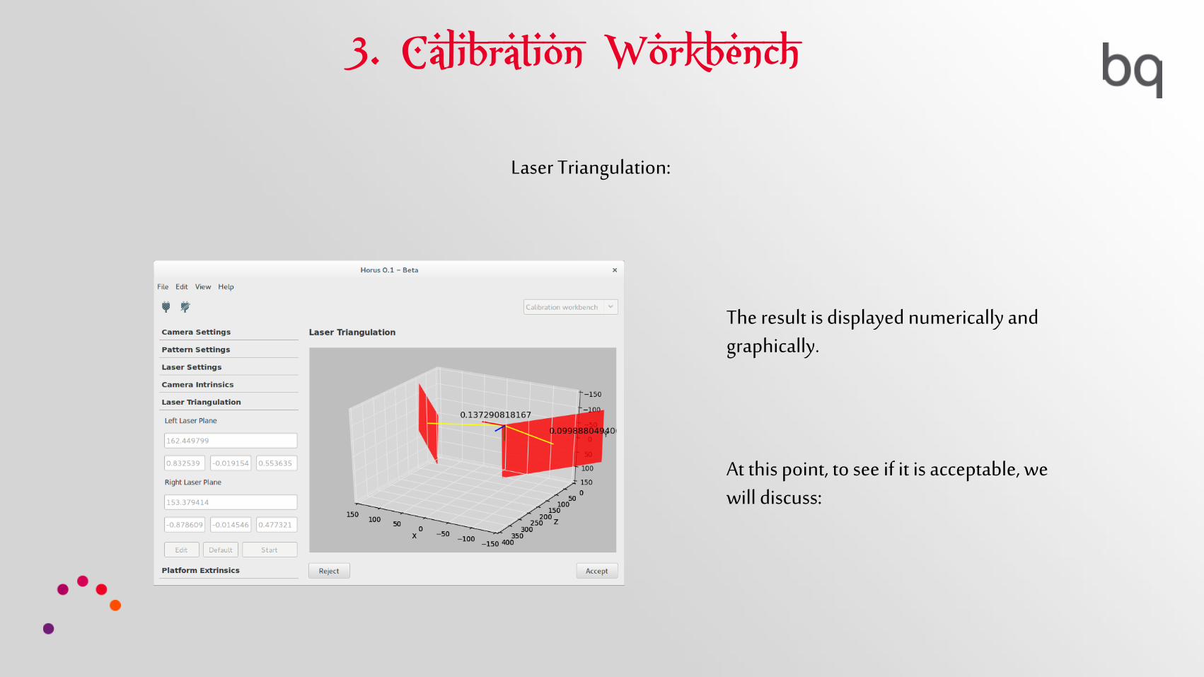
Laser Triangulation:
The result is displayed numerically and graphically.
At this point, to see if it is acceptable, we will discuss:

3. Calibration Workbench
Laser Triangulation:
1- Dispersion of points: Both numbers should be as close to 0.1.
2- Minimum distance from the plane to the origin: The difference should be less than 30

3. Calibration Workbench
Extrinsic Calibration:
The aim is to calculate:
• The position, and rotation of the disk center or platform
3. Calibration Workbench
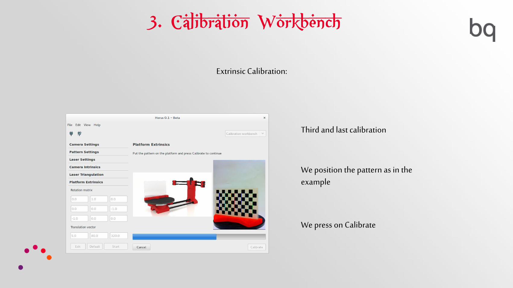
Extrinsic Calibration:
Third and last calibration
We position the pattern as in the example
We press on Calibrate

3. Calibration Workbench
Extrinsic Calibration:
The result is displayed numerically and graphically.
At this point, we can accept or reject the calibration.

4. Scanning Workbench
Scanning and obtaining the points cloud

4. Scanning Workbench
Configure the scanning options and you get the points cloud
4. Scanning Workbench
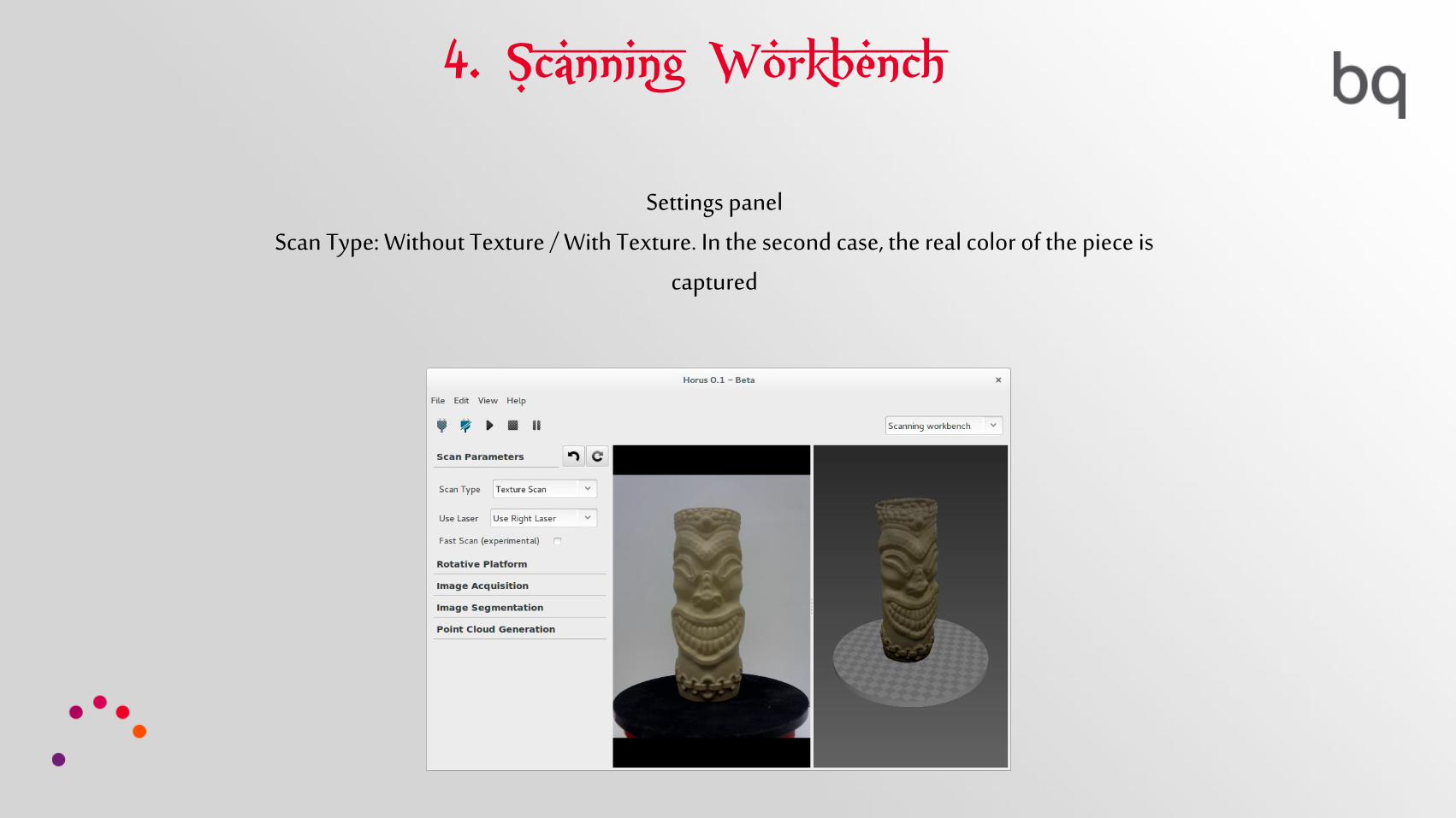
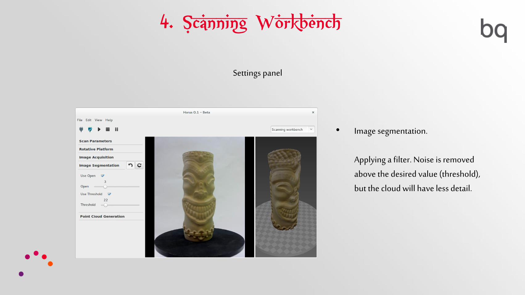
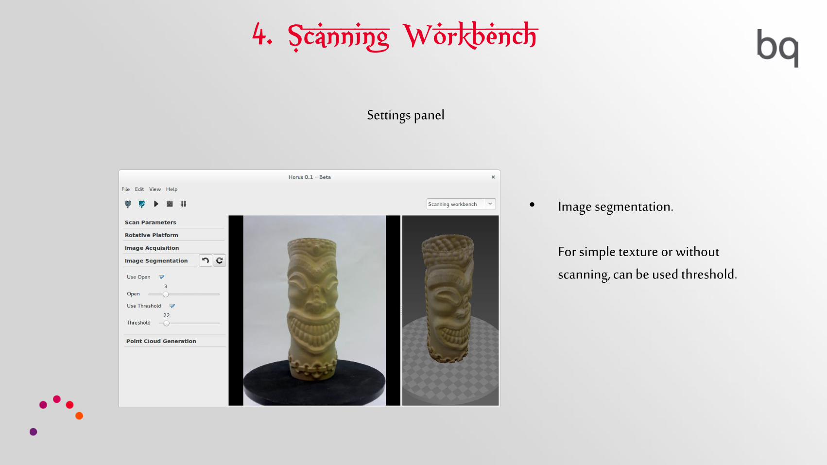
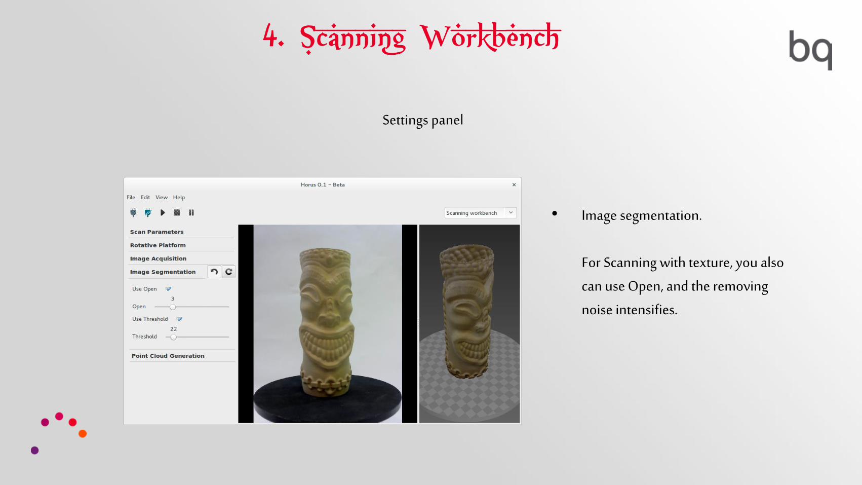
Settings panel
Scan Type: Without Texture / With Texture. In the second case, the real color of the piece is captured
4. Scanning Workbench
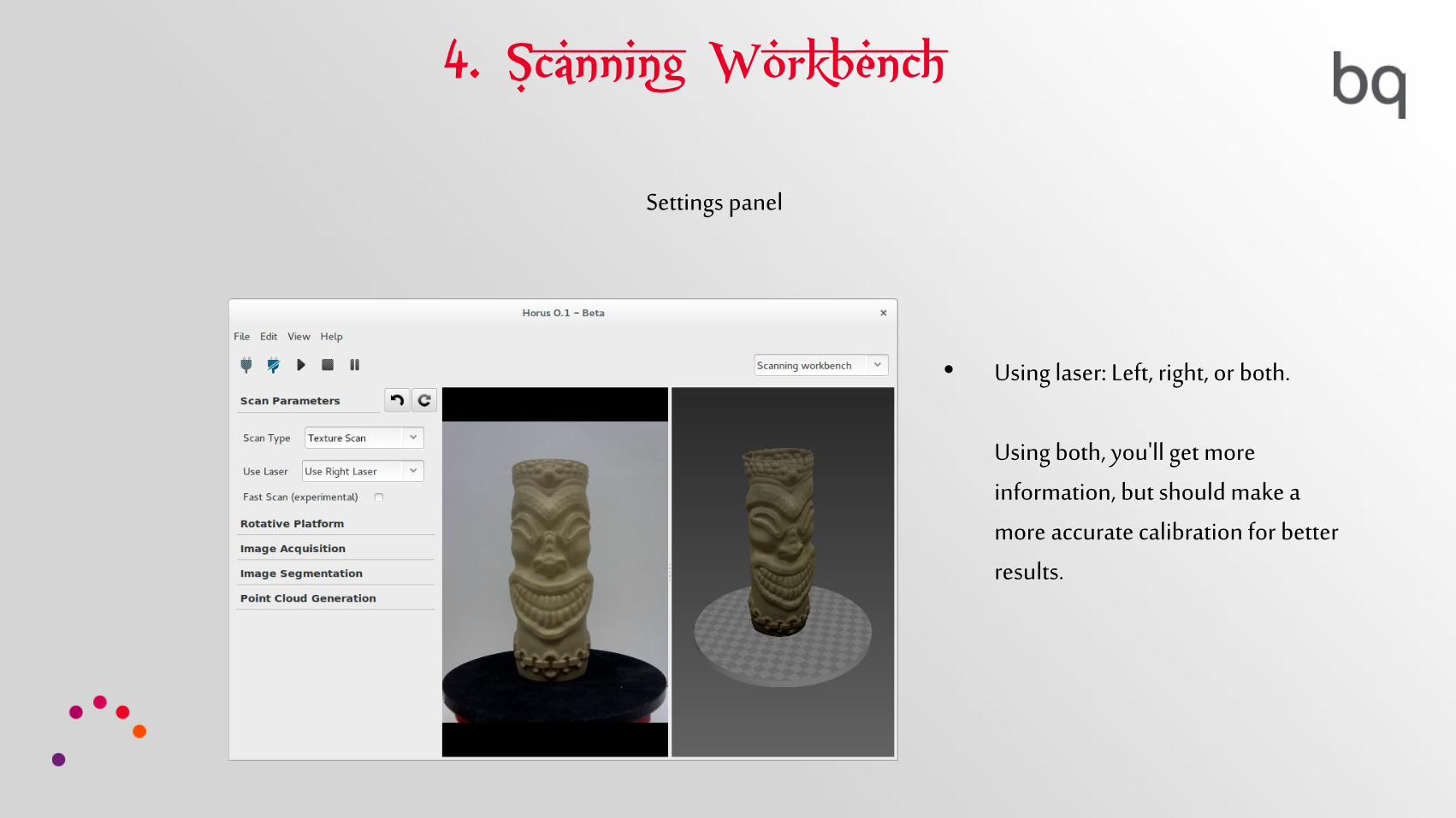
Settings panel
• Using laser: Left, right, or both.
Using both, you'll get more
information, but should make a
more accurate calibration for better results.
4. Scanning Workbench
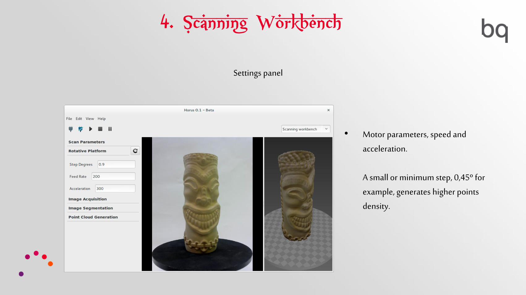
Settings panel
• Motor parameters, speed and
acceleration.
A small or minimum step, 0,45º for
example, generates higher points density.
4. Scanning Workbench
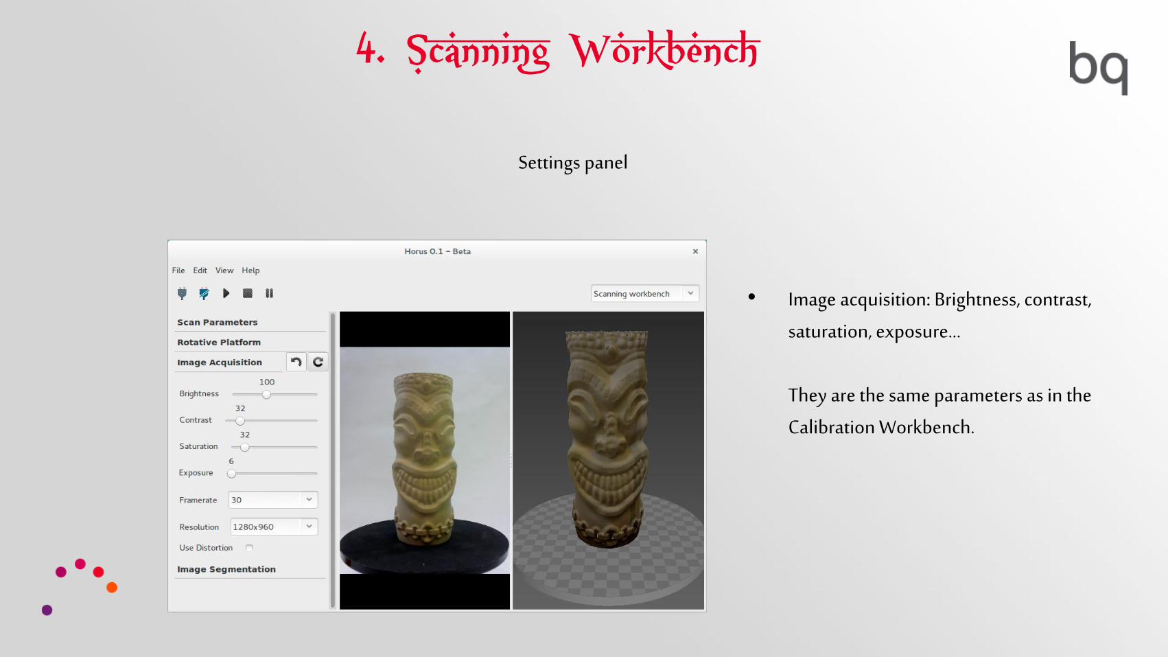
Settings panel
• Image acquisition: Brightness, contrast,
saturation, exposure...
They are the same parameters as in the
Calibration Workbench.
4. Scanning Workbench
Settings panel
• Image segmentation.
Applying a filter. Noise is removed
above the desired value (threshold),
but the cloud will have less detail.
4. Scanning Workbench
Settings panel
• Image segmentation.
For simple texture or without
scanning, can be used threshold.
4. Scanning Workbench
Settings panel
• Image segmentation.
For Scanning with texture, you also
can use Open, and the removing
noise intensifies.

4. Scanning Workbench
Settings panel
• ROI: Creating an area of interest.
It will be scanned only within the
cylinder, avoiding obtaining noise
from outer areas.

4. Scanning Workbench
Settings panel
To scan, press in the PLAY icon
Once finished, to save the point cloud will click on File > Save Model
The output format will be .PLY
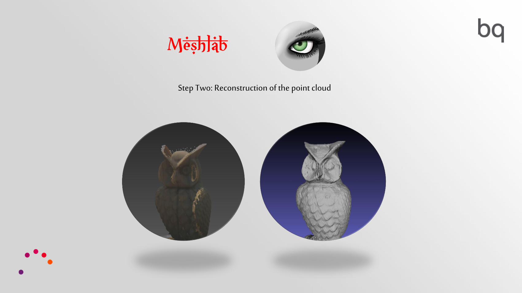
Meshlab
Step Two: Reconstruction of the point cloud

1. Cleaning the Cloud2. Calculation of normal vectors
3. Poisson Reconstruction
4. Joining clouds (optional)
5. Smoothing the .STL (optional)

1. Cleaning the Cloud
Cloud cleaning is use to remove those points that do not want, because they are noise, or do not
interest us
1. Cleaning the Cloud
To do this, we open the point cloud format .PLY
File > Import mesh
1. Cleaning the Cloud
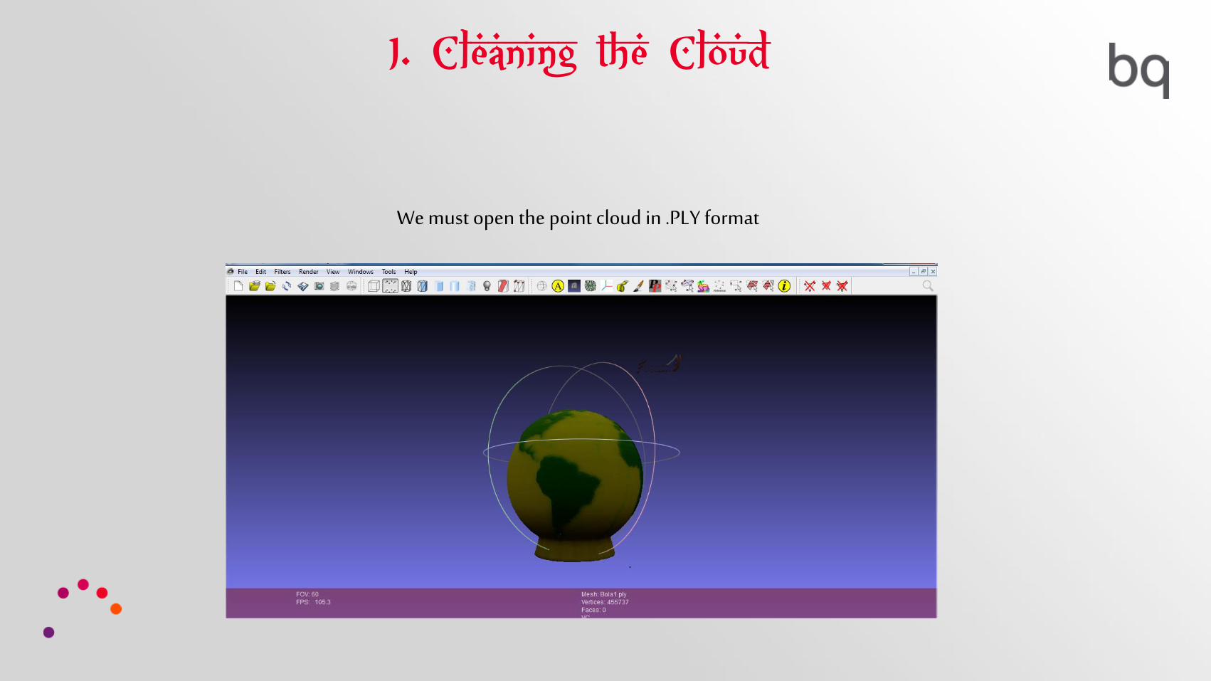
We must open the point cloud in .PLY format
1. Cleaning the Cloud
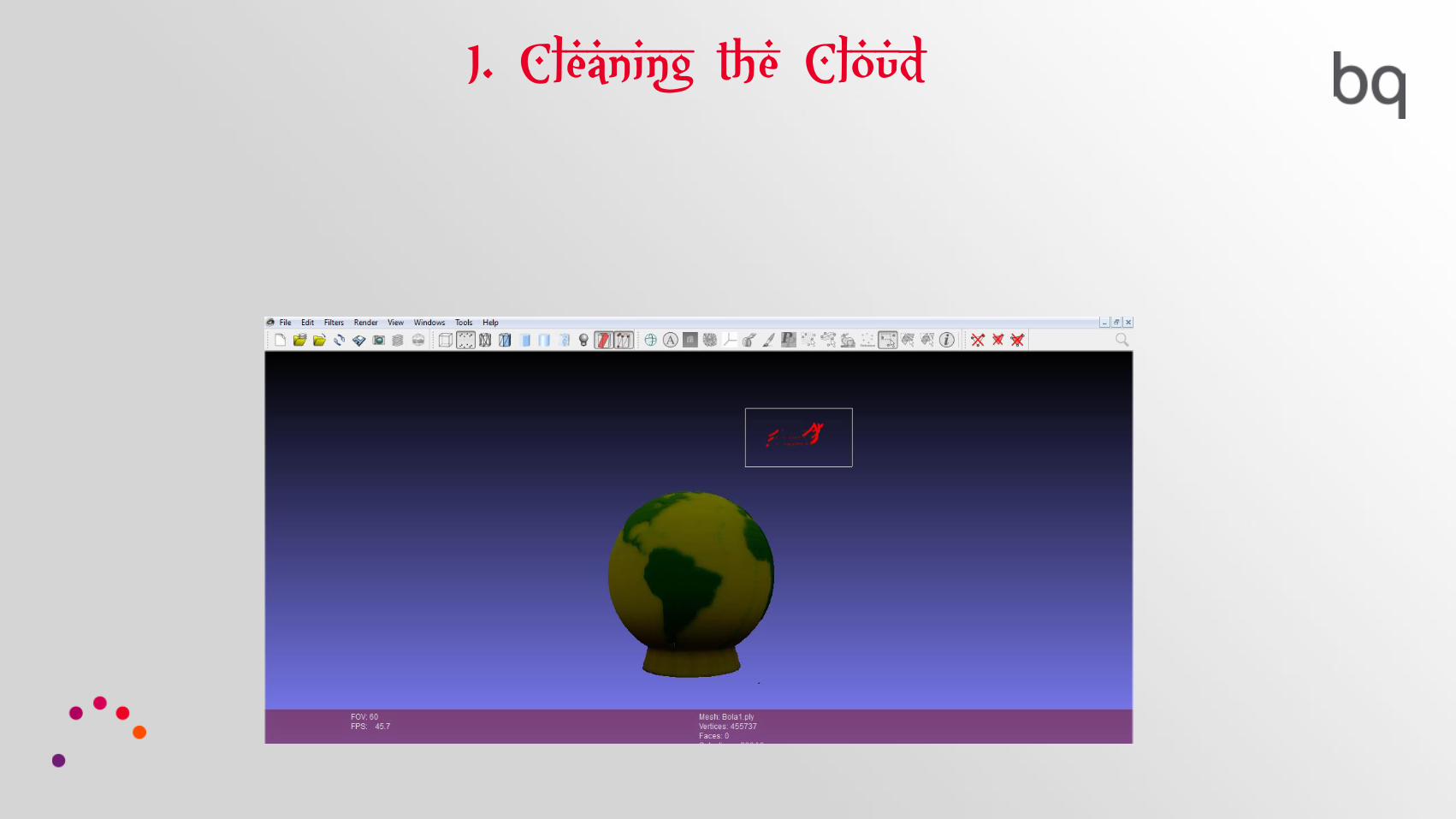
To delete points, select the Vertex Select tool
Then we choose the unwanted points. They are displayed in red
1. Cleaning the Cloud

1. Cleaning the Cloud
1. Cleaning the Cloud
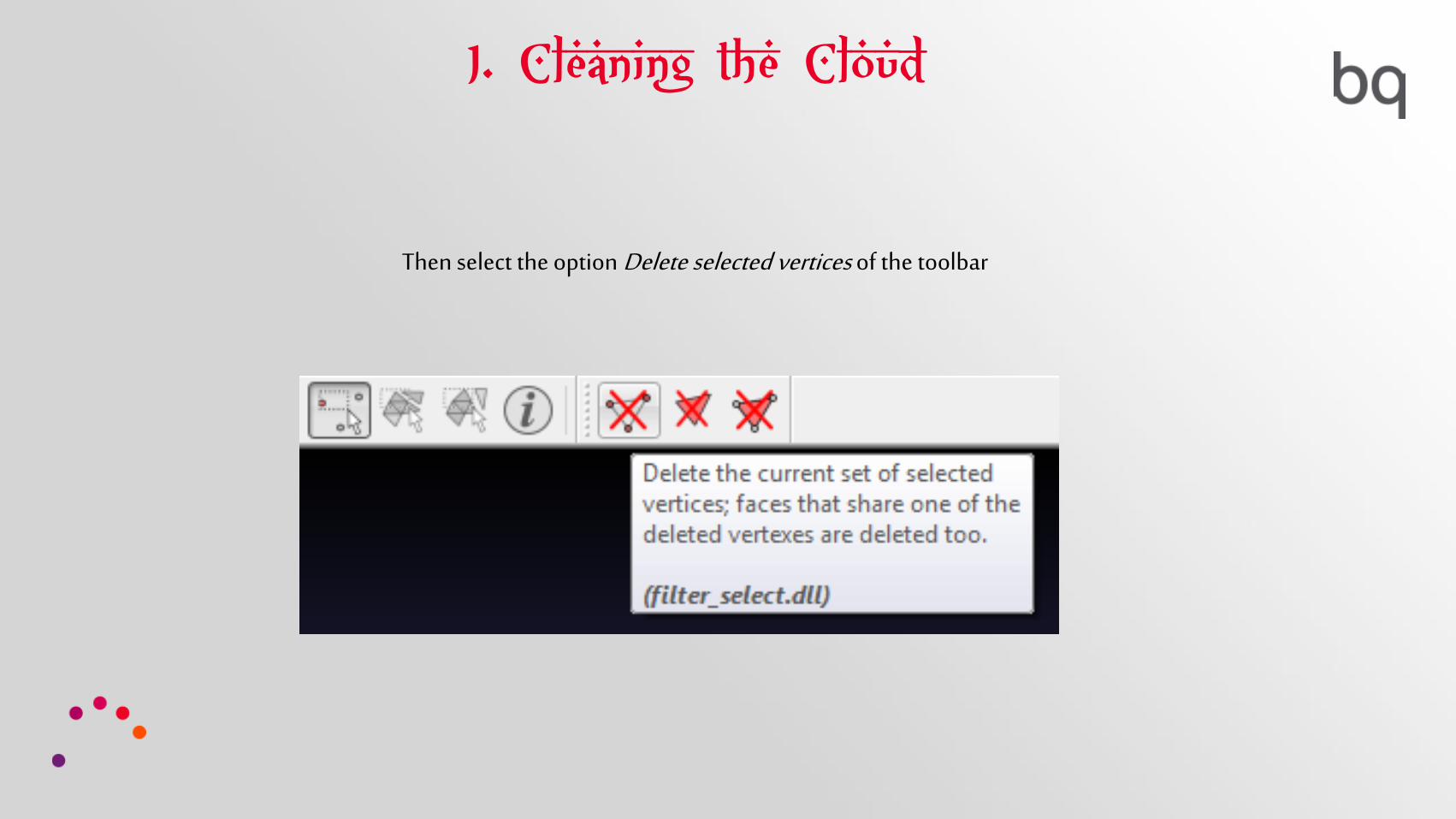
Then select the option Delete selected vertices of the toolbar
1. Cleaning the Cloud
A cleaned cloud points will be very important to obtain a good result

2. Calculation of normal vectors
A normal is a perpendicular vector to a plane
2. Calculation of normal vectors
In this step, we will calculate the normal of the points cloud.
To do this, we group a number of points to form a plane, and finally the average is calculated.

2. Calculation of normal vectors

2. Calculation of normal vectors
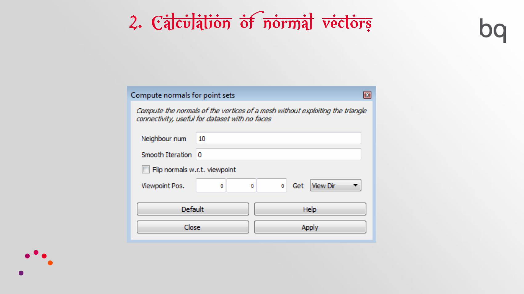
Now we calculate the number of neighbors. Determines the amount of points needed to create a vector.
It is recommended to start with a value of 10. The other values will be left by default. Then, we apply it.
2. Calculation of normal vectors

2. Calculation of normal vectors
We show normal. The best reconstructions are when the direction of the vectors are oriented away from the object.
If the normal vectors are not directed outwards, we repeat the step changing the number of neighbors to 50; if repeated, 100.

2. Calculation of normal vectors
Number of
neighbors: 10Number of
neighbors: 50

3. Poisson Reconstruction
For the reconstruction, we convert from .PLY to .STL
It is a critical step, because depending on the previously established normal and reconstruction values, the STL may vary.

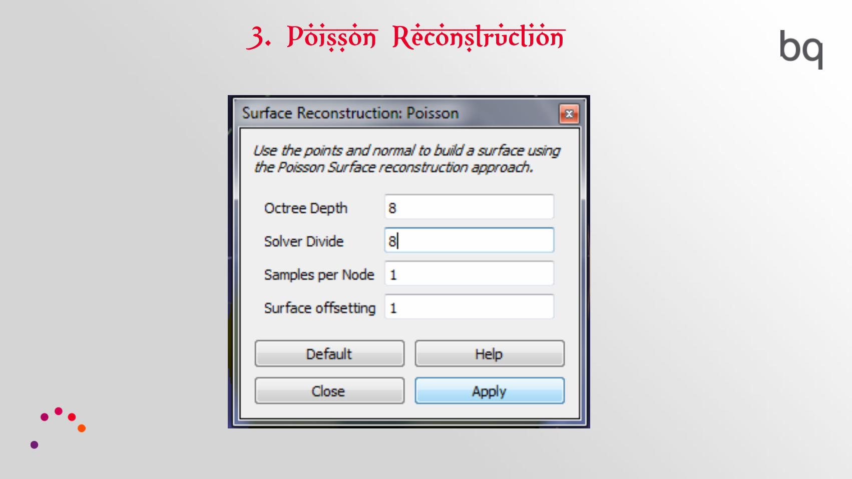
To do this, we choose the option Poisson Reconstruction
3. Poisson Reconstruction

3. Poisson Reconstruction
In this window you can modify two values:
3. Poisson Reconstruction
• Octree Depth• Solver Divide

The recommended values of both parameters are between 6 and 11.
With a higher the value, the reconstruction is more accurate, but it takes longer to make the process.
3. Poisson Reconstruction
3. Poisson Reconstruction

3. Poisson Reconstruction
To view reconstruction:
View > Show Layer Dialog

3. Poisson Reconstruction
3. Poisson Reconstruction
To save the reconstruction (STL):
File > Export Mesh…
3. Poisson Reconstruction
Sometimes due to the geometry of the piece, the cloud of points are incomplete.
To fix this, you can re-scan the piece in another position or by using another laser, and then join the different clouds.
4. Joining clouds (optional)
To do this, we will open the various .PLY in MeshLab
4. Joining clouds (optional)

4. Joining clouds (optional)
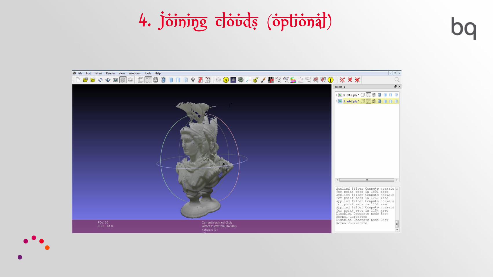
In the Layer Dialog, we calculate each normal point cloud, as described above.
Once done, we click on the Align tool

4. Joining clouds (optional)
4. Joining clouds (optional)
In the Tool panel, we click on the first layer, and we glue it at the space (Glue Here Mesh)
Then, we select the second mesh, and click on Point Based glueing.

4. Joining clouds (optional)

4. Joining clouds (optional)
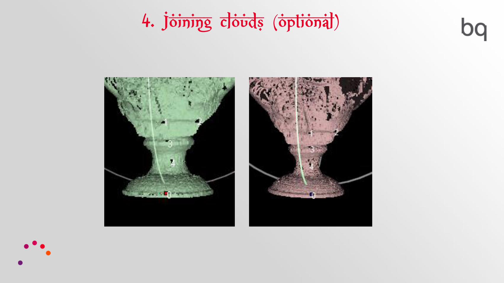
In this window you have to select at least 3 points in common of both clouds.
Example: First a point cloud 1, and then the same point in the 2nd.
The choice does not have to be exact, can be approximated.
4. Joining clouds (optional)
4. Joining clouds (optional)
The numbered points appear. If you select an invalid point you must cancel and repeat the process.
Once the points are selected, click on OK.

4. Joining clouds (optional)
4. Joining clouds (optional)
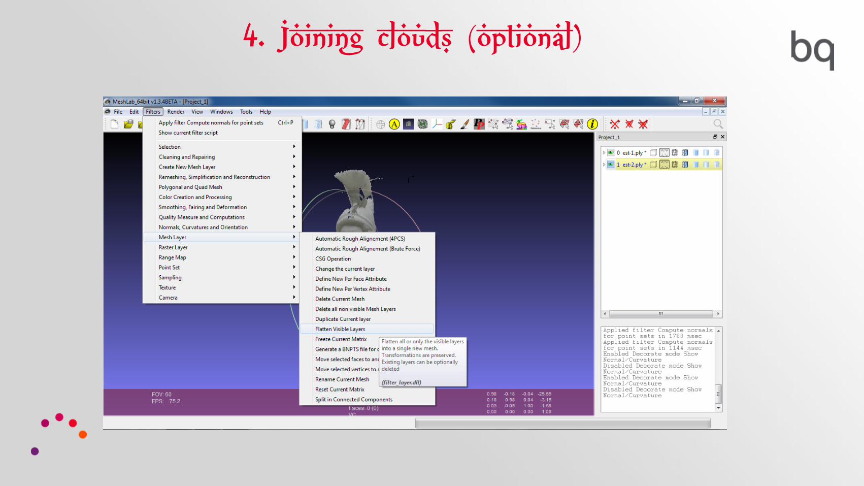
To join the aliened clouds:
Filters > Mesh Layer > Flatten Visible Layers
4. Joining clouds (optional)
4. Joining clouds (optional)
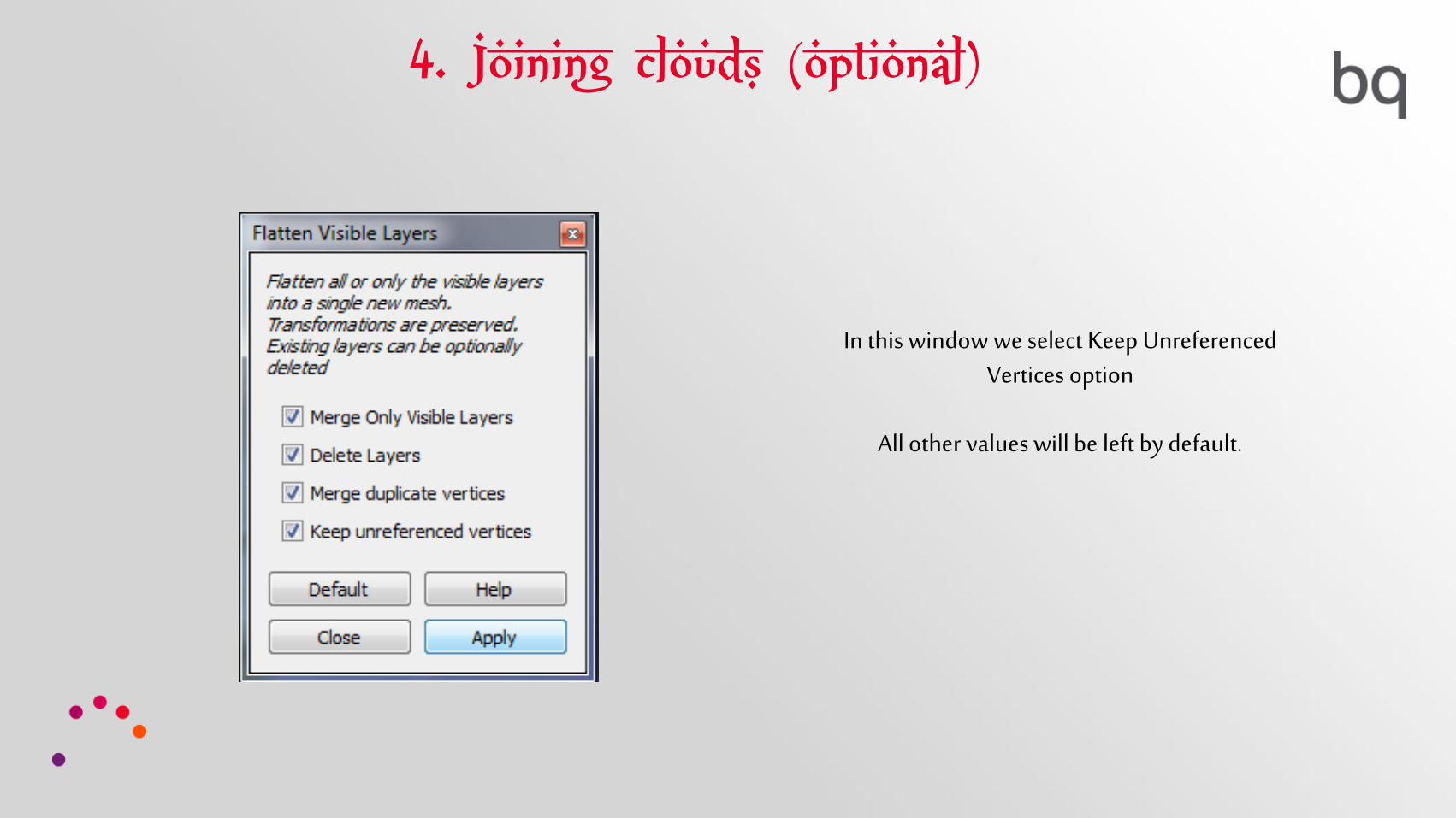
In this window we select Keep Unreferenced Vertices option
All other values will be left by default.

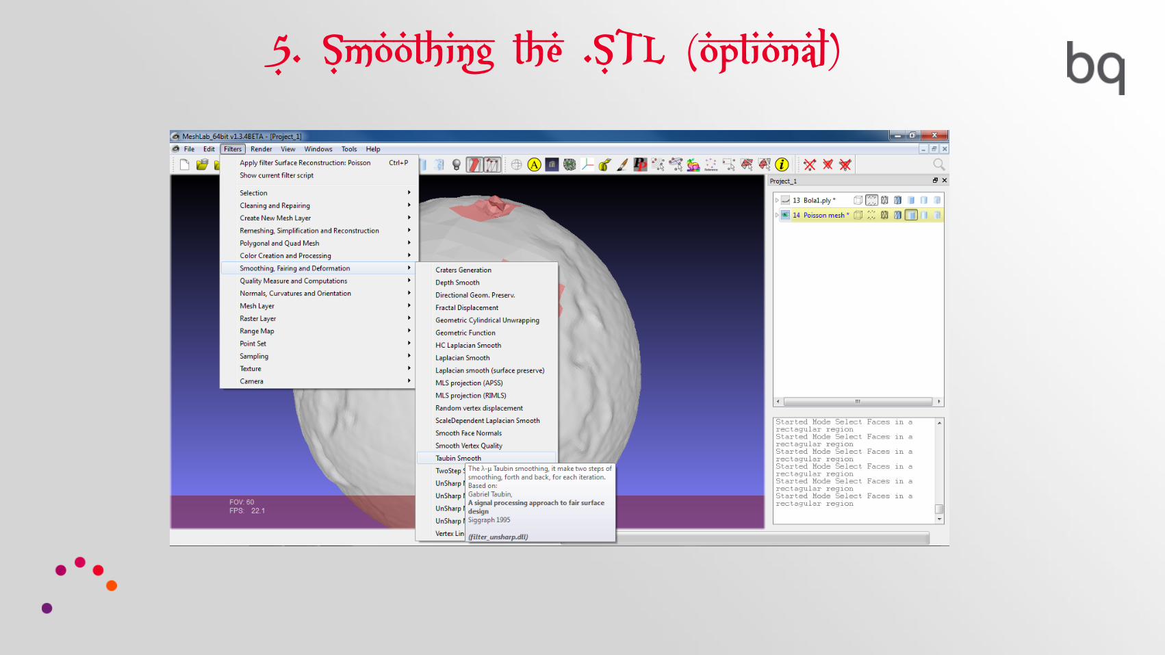
5. Smoothing the .STL (optional)
Although it is a process that can be performed with a different software, MeshLab gives the opportunity to smooth the STL reconstructed.

Our goal is to smooth the jagged faces
5. Smoothing the .STL (optional)

With the Selection tool faces, we select the faces that we choose to smooth, and then choose Smooth Taubin.
5. Smoothing the .STL (optional)

5. Smoothing the .STL (optional)
5. Smoothing the .STL (optional)

5. Smoothing the .STL (optional)
Lambda is by default.
About the rest of values, we recommend them as in the picture.

5. Smoothing the .STL (optional)
The result is the following: