J R E R � V o l . 3 0 � N o . 3 – 2 0 0 8

P r e s a l e s , F i n a n c i n g C o n s t r a i n t s , a n dD e v e l o p e r s ’ P r o d u c t i o n D e c i s i o n s

A u t h o r s Su Han Chan, Fang Fang, and Jing Yang

A b s t r a c t This study explores the impacts a presale contract has on adeveloper’s pricing and production decisions in a game-theoretical framework. In an environment where developershave full capital market access, the findings reveal that bothdevelopers and buyers are indifferent between a presale and aspot sale method. However, in an environment with financingconstraints, both developers and buyers are better off when apresale method is used. This is because the presale method solvesthe financing constraint by injecting equity into the developmentand, hence, reducing financing costs. This model predictionseems to describe well the real world situations seen in some ofthe property markets in Asia that have nascent financial systems.

The presale method has been a popular tool for selling properties in many Asiancountries for at least the past five decades.1 Under this method, a developer cansell a property before its completion (or even before its construction). However,even with more than five decades of experience with this system, we still do notknow much about its benefits (as compared to a spot sale at the completion of aproject), nor its impact on the market structure of the product market. Recently,the presale practice started to gain increasing attention in the United States asresidential property prices surged during the 2005–2006 period. For example, theLos Angeles Times (8/22/06) reported that, ‘‘In previous real estate cycles, there’sbeen lots of building...and builders and lenders were stuck with a lot of inventory... But new builders pre-sell just about every building they build. They are muchmore cautious.’’2 If so, the news story seems to suggest that the presale systembenefits developers by helping them unload their inventory in a speculative market.This is probably the case, as it confirms the report by Lai, Wang, and Zhou (2004)that the presale system offers developers an opportunity to share risks with buyers.

Although there has been growing research on Asian property markets, the presalemethod (which is very popular in Asia) has not received much attention in theacademic literature.3 We can find only a few studies that address this issue. Onegroup of studies treats a presale as a forward or futures contract (ignoring a buyer’soption to default) and addresses issues such as pricing factors (Chang and Ward,1993) and the relationship between presale pricing and future spot sale pricing

3 4 6 � C h a n , F a n g , a n d Y a n g

(Wong, Yiu, Tse, and Chau, 2006). Another stream of the literature treats a presaleas an option contract, and addresses issues such as its impacts on a developer’sdevelopment strategies (Lai, Wang, and Zhou, 2004) and its influence on marketstructure (Wang, Zhou, Chan, and Chau, 2000). Finally, Hua, Chang, and Hsieh(2001) demonstrate that, in addition to being viewed as a ‘‘stock’’ (inventory ofproperties) market, a presale market can be viewed as a ‘‘flow’’ market. Theauthors believe that, in the presale market, since trades can be made on propertiesin progress, the housing supply can be adjusted to catch the contemporaneousdemand change and economic outlook.

However, many unanswered questions about the presale method still remain. Ifthe primary function of the presale method is for developers to unload theirinventories in a speculative market (as described in the LA Times article) or forthem to share risks with buyers, then we need to know what impact this practicemight have on other market participants. Will the pre-sold inventories eventuallycreate problems for those who bought them from the developers? Should buyerswait and buy the properties in the spot market after the project is completed? Willdevelopers behave differently in their pricing and production decisions with andwithout the presale system? In addition, it is a popular belief in Asia that, sincethe debt markets are nascent, the presale system is a necessary tool for developersto obtain financing. Clearly, none of the existing studies has fully addressed theseissues.

In this paper, we provide a simple equilibrium model in a game-theoreticalframework to throw light on the relationship between presales and developers’pricing and production decisions.4 In this framework, a presale contract can beviewed as an option. That is, buyers have the right to buy a property at apredetermined exercise price and to default on the contract if the spot price divesbelow the contract price.5 Under this framework, we find that the presale methodper se does not affect a developer’s production decision. In equilibrium, developerswill increase the presale price to compensate for the option value they give to thebuyers. However, when we model the presale system under the condition thatdevelopers are facing financing constraints, we find a Pareto improvement fordevelopers and buyers. More importantly, we find that developers will tend toincrease the scale of their developments under the presale system. Our result seemsto conform to the high volume of development activities observed in those Asiancountries that lack a mature financial system, such as China.

We develop our benchmark model in Section 2. In Section 3, we explain why apresale contract can be viewed as an option, and show the relationship betweenthe level of downpayment and the presale price. We then model a developer’spricing and production decisions under financing constraints in Section 4. Section5 concludes.

� B e n c h m a r k M o d e l

In this model, we consider a risk-neutral representative developer who builds andsells a property within a time period t � [0, 1]. The construction starts at t � 0

P r e s a l e s , F i n a n c i n g C o n s t r a i n t s , a n d D e v e l o p e r s ’ � 3 4 7

J R E R � V o l . 3 0 � N o . 3 – 2 0 0 8

and finishes at t � 1. The developer can either pre-sell the property in the presalemarket at t � 0, or wait until t � 1 to sell the completed property in the spotmarket. To make the decision, at t � 0, the developer decides on 1) the optimalquantity q and associated price pp that will give him the maximum expectedpresale profit E(�)�presale, and 2) the optimal quantity qn and associated price pn

that will give him the maximum expected spot sale profit E(�)�spot. ComparingE(�)�presale and E(�)�spot, the developer chooses the selling approach that brings himthe higher expected profit. The property will then be constructed at a constantaverage cost c. We assume that in the presale (but not in the spot sale) thedeveloper will incur a project-specific fixed cost K, which can be considered as aspecial cost of using the presale method.

We also consider a risk-neutral representative buyer for this property. At t � 0,after observing the presale price pp, the buyer will decide to either accept or rejectthe presale offer. Upon rejection, the buyer needs to wait until t � 1 to buy theproperty in the spot market at price p1. Upon acceptance, however, she needs tomake an immediate downpayment, which is assumed to be a percentage, d, of thepresale price pp. The balance will be paid at t � 1 upon delivery of the property.Of course, the buyer can also decide not to purchase the presold property if shebelieves that she can buy it cheaper in the open market.

For simplicity, we assume a linear and inverse demand function p1 � a � z �bq, which will be realized at t � 1. In this function, a is the base demand and zis the market demand shock that remains unknown until t � 1. However, at t �0, it is common knowledge that z is in the range [ � �, � �] with a probabilityz zdistribution function �(z). b is the property’s price elasticity to quantity. To preventa negative market price, we assume that a is significantly larger than otherparameters in the demand function.

Note that at t � 0, a buyer’s accept-reject decision towards the presale offer ismade under uncertainty about the market demand shock z. At t � 1, when themarket demand shock is realized at z and a market price is formed at p1 � a �z � bq, the buyer’s follow-up decision is either to pay the presale balance, whichequates to the compounded value of the unpaid portion of the presale price,[(1 � d)pp](1 � i), or to default and buy the completed property in the spot marketat price p1. Intuitively, the buyer may have an incentive to default if the realizeddemand shock z is low enough to generate an attractive spot price p1. Finally, wealso assume that the risk-free rate i is positive; in other words, there is a timevalue of money.

The whole model involves three major steps: (1) the developer’s decision at t �0 on the optimal development size and price under each selling approach; (2) thebuyer’s decision at t � 0 on whether or not to accept the presale deal; and (3) thebuyer’s decision at t � 1 on whether or not to continue with the presale paymentif she has accepted the presale offer. Exhibit 1 summarizes those decision rulesin a step-by-step fashion, while Exhibit 2 summarizes the payoff for each routetaken by the developer and the buyer.

3 4 8 � C h a n , F a n g , a n d Y a n g

Exhibi t 1 � Game Tree for the Benchmark Model

Buyer

Accept presale Reject presale

PAS

Pay [(1 – d )pp](1 + i) Default

q and pp

Downpayment d pp

Buyer

Developer Developer

PR

Offer presale Does not

offer presale

N

qn

Sell qn at pn = a + z-bqn

Sell q at p1 = a +

Developer

Demand shock is realized at z

Demand shock is realized at z

Demand shockis realized at z

PAC

Sell q at p1 = a + z-bq z-bq

t = 0

t = 1

Demand shock

],[~~ σσ +−Φ zzz

The game covers two time periods: t � 0 and t � 1. The demand shock z is unknown until t � 1. However,from t � 0, its distribution z � �[ � �, � �] is already known by the public. At t � 0, a developer decidesz zto either immediately offer a presale contract with a property size q and a price pp, or build a property with sizeqn and put it in the spot market at t � 1 with market clearing price pn � a � z-bqn. Upon a presale, a buyerdecides to either accept the offer and pay the downpayment d pp or reject the offer. At t � 1, upon acceptingthe presale offer, the buyer decides to either pay the compounded value of the balance of the payment [(1 �

d)pp](1 � i), or default on the payment; upon rejecting the presale offer or accepting it first but defaulting later,the buyer will switch to the spot market at t � 1 to buy the property from the developer at market clearing pricep1 � a � z-bq. The game ends at terminal nodes PAC, PAS, PR or N, respectively, when a committed presale,a defaulted presale, a rejected presale or a spot sale occurs.

Pr

es

al

es

,F

in

an

ci

ng

Co

ns

tr

ai

nt

s,

an

dD

ev

el

op

er

s’

�3

49

JR

ER

�V

ol

.3

0�

No

.3

–2

00

8

Exhibi t 2 � Outcomes and Payoffs

TerminalNode

Developer’sOffer Type Buyer’s Action

Final SaleType Each Buyer’s NPV Developer’s NPV

PAC Presale Accept offer,commit

Presale pp (pp � c)q � K

PAS Presale Accept offer,default

Spot saledpp � (a � z � bq)

1(1 � i)

1dp � (a � z � bq) � c q � K� �p (1 � i)

PR Presale Decline offer Spot sale(a � z � bq)

1(1 � i)

1(a � z � bq) � c q � K� �(1 � i)

N Spot sale Accept offer Spot sale(a � z � bqn)

1(1 � i)

1(a � z � bq ) � c q� �n n(1 � i)

Notes: This table summarizes all the possible outcomes and the corresponding payoffs for each buyer and the representative developer. PAC, PAS, PR, andN are the indexes for outcomes (see Exhibit 1), each matched with a set of decisions; pp and q are the price and quantity under a presale; qn is the quantityunder a spot sale; c is the construction cost per unit; i is the risk-free rate; K is the additional transaction cost associated with presales; z is the uncertaindemand shock; a is the base demand; and b is the price elasticity of quantity.

3 5 0 � C h a n , F a n g , a n d Y a n g

The following sub-sections present the major procedure of solving this model withbackward induction. This means we will assume that the buyer has signed apresale contact and will first look at her decision (at t � 1) on whether to continuewith the presale contract.

A t t � 1 : B u y e r ’s D e c i s i o n t o C o n t i n u e o r D e f a u l t o n aP r e s a l e C o n t r a c t

This subgame exists contingent upon the developer’s presale offer and the buyer’spresale acceptance. After observing the demand shock z, the buyer will decide toeither pay the presale balance [(1 � d)pp](1 � i), or default and buy the propertyat its spot price p1. Given that the previous downpayment is a sunk cost, the buyerwill compare the present value of her incremental cost from continuing with thepresale payment versus that from defaulting, or:

�C� � [(1 � d)p ](1 � i), (1)continue p

�C� � p � a � z � bq. (2)default 1

Her sufficient and necessary condition to continue with the presale payment is:�C�continue � �C�default, that is:

z � z � � a � bq � (1 � d)(1 � i)p , (3)p

where z is the demand shock level that makes the buyer indifferent between thesetwo options and any demand shock higher than this level will induce a fullpayment. Note that we can derive:

�z� �(1 � i)p � 0. (4)p�d

Intuitively, when the downpayment percent d is higher, the loss of downpaymentupon default is also higher. This gives the buyer more incentive to continue withher payment and to follow through with the presale contract.

P r e s a l e s , F i n a n c i n g C o n s t r a i n t s , a n d D e v e l o p e r s ’ � 3 5 1

J R E R � V o l . 3 0 � N o . 3 – 2 0 0 8

A t t � 0 : B u y e r ’s D e c i s i o n t o B u y a t P r e s a l e o r S p o tM a r k e t

The existence of this part of the subgame depends on the developer’s decision tomake a presale offer. At t � 0, the demand shock z is not realized yet. The presentvalue of the buyer’s expected total cost if she accepts the presale offer is:

z��

E(C)� � � p d�(z)accept pz

z 1� � dp � (a � z � bq) d�(z). (5)� �p

z�� (1 � i)

The first integral is the present value of her expected cost if she later (at t � 1)chooses to continue with the presale contract. The second integral is the presentvalue of her expected cost if she later defaults and goes to the spot market. Incontrast, the present value of her expected total cost if she declines the presaleoffer at t � 0 and waits until t � 1 to buy the property in the spot market is:

z�� 1E(C)� � � (a � z � bq)d�(z). (6)decline

z�� (1 � i)

Her sufficient and necessary condition to accept the presale offer at t � 0 is:

E(C)� � E(C)� . (7)accept decline

To simplify the presentation we assume that z follows a uniform distribution onsupport [ � �, � �]. The mathematical result for the buyer’s condition toz zaccept the presale offer is:

a � z � bqp � p (q) �p p (1 � d)(1 � i)

(1 � d)� � 2d�[� � (1 � d)(a � z � bq)]� .2(1 � d) (1 � i)

(8)

3 5 2 � C h a n , F a n g , a n d Y a n g

That is, if the presale price is no higher than then the presale offer will bep (q),p

accepted.

A t t � 0 : D e v e l o p e r ’s D e c i s i o n t o U s e a P r e s a l e o r a S p o tS a l e M e t h o d

With backward induction, which takes into account the buyer’s decision onwhether to accept the presale contract as well as her decision on whether tocontinue with the payment if she has accepted the presale offer, the developerchooses a selling method (a presale or a spot sale) for his development project.This choice also includes his decisions on the optimal quantity under each sellingmethod as well as the price if he were to offer a presale contract.

Consequently, this subgame involves two optimization steps. The first is to findthe optimal quantity (and price) under each of the two selling methods. The secondis to select between the presale method and the spot sale method. With theprevious subgame results given, the developer upon making a presale offer knowsthat the buyer will accept the offer only if the offer package satisfies pp �

p (q).p

This is the case since the developer will not have an incentive to make a presaleoffer that is deemed to be rejected. As a result, the only effective options left forthe developer at the beginning of the game is to offer either a spot-sale deal oran acceptable presale deal that satisfies pp � The developer’s optimization

p (q).p

problem for offering an acceptable presale deal is, therefore:

z��

E(�)� � max � p qd�(z)presale pz{p ,q}p

z 1� � [dp q � (a � z � bq)q]d�(z)p

z�� (1 � i)

�cq � K, (9)

where z � �a � bq � (1 � d)(1 � i)p ,p

a � z � bqs.t. p � p (q) �p p (1 � d)(1 � i)

(1 � d)� � 2d�[� � (1 � d)(a � z � bq)]� .2(1 � d) (1 � i)

Here, E(�)�presale defines the present value of the developer’s expected payoff fromoffering a presale contract, where ppqd�(z) is the present value of hisz���z

P r e s a l e s , F i n a n c i n g C o n s t r a i n t s , a n d D e v e l o p e r s ’ � 3 5 3

J R E R � V o l . 3 0 � N o . 3 – 2 0 0 8

expected development revenue if the buyer continues with the payment, z�z��

[dppq � 1/(1 � i) (a � z � bq)q]d�(z) is the present value of the developer’sexpected development revenue if the buyer stops payment at a later stage (underthis circumstance, the developer has to sell the property in the spot market whenit is completed), cq is the development cost for the presale property, and K is thepresale associated cost. Finally, the pricing is subjected to the constraint pp �

(q).pp

Alternatively, given the projected demand function (p1 � a � z � bq), thedeveloper can select an optimal price pn and an optimal quantity qn to sell theproject in the spot market. For this option, the developer will solve:

z�� 1E(�)� � max � p � c q d�(z),�� � �spot n n

z�� (1 � i){q }n

(10)

where p � a � z � bq .n n

Here, E(�)�spot defines the present value of the developer’s expected payoff if hedecides to sell the property on the spot at t � 1. Note that the buyer’s expectedcost from this spot sale will be:

z�� pnE(C)� � � d�(z),spotz�� (1 � i)

(11)

where p � a � z � bq .n n

After solving for the optimal prices and quantities under the two selling methods(presale versus spot sale), the developer compares the expected net present valuesfor these two choices, E(�( ))�presale versus E(�( ))�spot, and chooses thep*, q* p*, q*p p n n

presale method only if:

E(�(p*, q*))� � E(�(p*, q*))� . (12)p p presale n n spot

Exhibit 3 summarizes the decision rules of the developer and the buyer. Theequilibrium outcomes are presented in Proposition 1.

Proposition 1. In equilibrium, the optimal price and optimal quantity of a presalecontract are:

35

4�

Ch

an

,F

an

g,

an

dY

an

g

Exhibi t 3 � Decision Rules

Developer’s NPVComparisons Sale Choice Price Condition

Buyer’s Responseto Offer

Realized DemandShock

Buyer’s DefaultDecision

TerminalNode

E (� ( ))�presalep*, q*p p

�

E (� ( ))�spotp*, q*n n

Presale p* � p (q*)p p p

p* � p (q*)p p p

AcceptDecline

z � zz � z—

No defaultDefault

—

PACPASPR

E (� ( ))�presalep*, q*p p

�

E (� ( ))�spotp*, q*n n

Spot sale — Accept — — N

Notes: This table summarizes the decision rules for the developer and the buyer. PAC, PAS, PR, and N are the indexes for outcomes (see Exhibit 1); E (�) isthe developer’s expected NPV from offering property sales; and are the optimal price and quantity under a presale; is the optimal quantity (with ap* q* q*p p n

corresponding price ) under a spot sale; ( ) � a � � /(1 � d)(1 � i) � (1 � d)� � 2 /(1 � d)2(1 � i) is the

p* p q* z bq* d�[� � (1 � d)(a � z � bq*)]n p p p p

ceiling for the presale price to avoid a rejection from the buyer; and z � �a � � (1 � d)(1 � i) is the ceiling for the demand shock to avoid abq* p*p p

default on presale payment.

P r e s a l e s , F i n a n c i n g C o n s t r a i n t s , a n d D e v e l o p e r s ’ � 3 5 5

J R E R � V o l . 3 0 � N o . 3 – 2 0 0 8

a � z � c(1 � i)q* � , and (13)p 2b

a � z � c(1 � i)p* �p 2(1 � d)(1 � i)

�(1 � d) � 2d�[(1 � d)(a � z � c(1 � i)) � 2�]� . (14)2(1 � d) (1 � i)

The optimal price and optimal quantity of a spot sale contract are:

a � z � c(1 � i)q* � , and (15)n 2b

a � z � c(1 � i)p* � . (16)n 2

Thus, the development scale is the same under both selling methods, with:

q* � q*. (17)p n

Ignoring the presale-specific transaction cost K, a developer is indifferent betweenoffering a presale or a spot sale, with:

E(�(p*, q*))� � E(�(p*, q*))�p p presale n n spot

2[a � z � c(1 � i)]� . (18)

4b(1 � i)

Finally, a buyer’s expected cost of buying the property should be the sameregardless of the selling method used by the developer, with:

E(C(p*, q*))� � E(C(p*, q*))�p p accept p p decline

a � z � c(1 � i)� E(C(p*, q*))� � . (19)n n spot 2(1 � i)

3 5 6 � C h a n , F a n g , a n d Y a n g

Proof. See Appendix A. �

These results are very interesting. When a presale serves only as a method to sellproperties, it does not affect the fundamental supply and demand in the underlyingmarket (meaning that developers will not alter their production decisions basedon the presale result, nor will buyers change their demand curves). Under thisscenario, the presale method will not affect the development scale (and theassociated marketclearing price), the market structure, nor the developer’s welfare.When the presale-specific transaction cost is very trivial, the developer willbe indifferent between a presale contract and a spot sale. In other words, whenthe presale-specific transaction cost is non trivial, the developer will prefer a spotsale.

In addition, a presale will not impact the buyer’s welfare either. As compared toa spot sale, a presale will provide the buyer flexibility after a demand shock occurs.If the demand shock is small such that the spot price is relatively lower than thepresale commitment (i.e., the compounded residual payments for the presale), thebuyer will default on the presale payment and switch to the spot market. However,this flexibility is not free and its costs include a downpayment and a pricedifference between the two contracts, which we will discuss in the next section.In an efficient market, this flexibility will be fully priced, and as such the buyer’sexpected purchase cost will be the same as in a spot sale.

� D o w n p a y m e n t a s a n O p t i o n

In essence, a presale contract gives a buyer a call option (at t � 0) to buy thecompleted project in the next period (at t � 1) at a contract price (which shouldbe lower than the spot market price). Given this, the downpayment can beconsidered as a part of the cost of this option, while the strike price is the residualpayment specified in the presale contract. When the project is completed at t �1, a spot price higher than the residual payment will trigger an exercise of thiscall option. In contrast, if the spot price is lower than the residual payment, thenthe call option will not be exercised. Under this circumstance, the buyer will buythe property in the spot market. Given this, it is interesting to investigate therelationships between the presale downpayment and the presale-spot sale pricespread.

O p t i o n a n d i t s C o s t

Comparing the presale price [in Equation (14)] and the spot price [in Equation(16)], we derive the present value of the presale-spot sale price spread as:

P r e s a l e s , F i n a n c i n g C o n s t r a i n t s , a n d D e v e l o p e r s ’ � 3 5 7

J R E R � V o l . 3 0 � N o . 3 – 2 0 0 8

1�p � p* � p*p n(1 � i)

1� {(1 � d)d[a � z � c(1 � i)]2 22(1 � d) (1 � i)

� 2(1 � i)�(1 � d)

� 2(1 � i)2d�[(1 � d)(a � z � c(1 � i)) � 2�]} � 0.(20)

This is true because:

2[(1 � d)d[a � z � c(1 � i)] � 2(1 � i)�(1 � d)]2� [2(1 � i)2d�[(1 � d)(a � z � c(1 � i)) � 2�]]

2 2 2� (1 � d) (1 � i) [d(a � z � c(1 � i)) � 2�] � 0. (21)

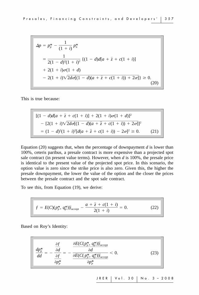
Equation (20) suggests that, when the percentage of downpayment d is lower than100%, ceteris paribus, a presale contract is more expensive than a projected spotsale contract (in present value terms). However, when d is 100%, the presale priceis identical to the present value of the projected spot price. In this scenario, theoption value is zero since the strike price is also zero. Given this, the higher thepresale downpayment, the lower the value of the option and the closer the pricesbetween the presale contract and the spot sale contract.

To see this, from Equation (19), we derive:

a � z � c(1 � i)ƒ � E(C)(p*, q*))� � � 0. (22)p p accept 2(1 � i)

Based on Roy’s Identity:

�E(C(p*, q*))��ƒ p p accept

dp* �d �dp� � � � � 0. (23)

�E(C( p*, q*))�dd �ƒ p p accept

�p* �p*p p

3 5 8 � C h a n , F a n g , a n d Y a n g

Intuitively, a buyer’s cost in a presale contract increases in the presale price andthe downpayment percentage. That is, �E(C( ))�accept /�d � 0 and �E(C(p*, q* p*,p p p

))�accept /� � 0. Given this, Equation (23) results in /dd � 0. Since spotq* p* dp*p p p

price is unaffected by presale downpayment d, we know that:p*n

1d p* � p*� �p n(1 � i) dp*d�p p

� � � 0. (24)dd dd dd

The negative interaction between the downpayment and the price spread ( � 1/p*p(1 � i) ) indicates a substitution relationship. In other words, to attract a buyerp*nto accept a presale contract with a higher downpayment, the developer will haveto reduce the presale price to compensate for the loss of some option value.Because of this substitution effect, the downpayment ratio will only affect theprice of the presale contract, but not the developer’s profit (and, hence, hisproduction decision). This relationship can be easily seen from Equations (18),(19), and (17), where d does not have an impact on E(�( ))�presale, E(�(p*, q* p*,p p n

))�spot, E(C)( ))�accept, E(C( ))�decline, , orq* p*, q* p*, q* q* q*.n p p p p p n

R e f u n d P o l i c y

In the real world, it is not uncommon to find a buyer in a presale contract askingthe developer to refund all or part of the downpayment when the property pricedrops below the presale price at the time of exercise. The buyer normally doesthis by complaining about construction quality and/or by accusing the developerof not building the property according to the specifications listed in the contract.It is possible that a developer is willing to refund part of the downpayment justto avoid a long legal battle and/or possible reputation damage.

Given this, we now analyze the developer’s decision under a refund possibility.We assume that the refund policy is known to both the buyer and the developerat the beginning period (t � 0) and the refund is calculated as a percentage x ofthe initial downpayment.

With a refund percentage x, the buyer’s decision at t � 1 on whether to defaultinvolves comparing the present values of her incremental costs associated withthe two choices:

P r e s a l e s , F i n a n c i n g C o n s t r a i n t s , a n d D e v e l o p e r s ’ � 3 5 9

J R E R � V o l . 3 0 � N o . 3 – 2 0 0 8

�C� � [(1 � d)p ](1 � i), and (25)continue p

�C� � p � a � z � bq � xdp . (26)default 1 p

The necessary and sufficient condition to continue with the presale payment is�C�continue � �C�default, or:

z � z � �a � bq � [(1 � d)(1 � i)]p , where (27)p

xd � d 1 � . (28)� �1 � i

Comparing the demand shock turning point z defined in Equation (27) with thatdefined in Equation (3), we can see that the only difference is that d is replacedby d.

With a refund, the present value of a buyer’s expected total cost if she acceptsthe presale offer is:

z�� z

E(C)� � � p d�(z) � �accept pz z��

1dp � (a � z � bq � xdp ) d�(z)� �p p(1 � i)

z�� z

� � p d�(z) � �pz z��

1dp � (a � z � bq) d�(z), (29)� �p (1 � i)

which differs from the expected cost without refund [as shown in Equation (5)]only in that d is replaced by d. Consequently, the decision rule with a refundshould also be similar to that with no refund [as shown in Equation (8)].

3 6 0 � C h a n , F a n g , a n d Y a n g

With a refund, the present value of the developer’s presale offer is:

z��

E(�)� � max � p qd�(z)presale pz{p ,q}p

z 1� � [dp q � (a � z � bq � xdp )q]d�(z)p p

z�� (1 � i)

� cq � K

z��

� max � p qd�(z)pz{p ,q}p

z 1� � [dp q � (a � z � bq)q]d�(z)p

z�� (1 � i)

� cq � K,

where

z � �a � bq � (1 � d)(1 � i)p ,p

xd � d 1 � ,� �1 � i

a � z � bqs.t. p � p (q) �p p (1 � d)(1 � i)

(1 � d)� � 2d�[� � (1 � d)(a � z � bq)]� .2(1 � d) (1 � i)

(30)

This differs from the present value of the developer’s presale offer (without arefund) only in that d is replaced by d. In fact, a refund actually reduces thedownpayment ratio from d to d � d(1 � x /(1 � i). Given this, the equilibriumpresale price in Equation (14) is changed to:

a � z � c(1 � i)p* �p 2(1 � d)(1 � i)

�(1 � d) �2d�[(1 � d)(a � z � c(1 � i)) � 2�]

� , (31)2(1 � d) (1 � i)

xwhere d � d 1 � .� �1 � i

P r e s a l e s , F i n a n c i n g C o n s t r a i n t s , a n d D e v e l o p e r s ’ � 3 6 1

J R E R � V o l . 3 0 � N o . 3 – 2 0 0 8

Following Equations (23) and (24), we find that:

dp*p � 0, (32)dd

1d p* � p*� �p n(1 � i) dp*d�p p

� � � 0, (33)dd dd dd

and correspondingly, the impacts of a refund percentage x on the presale priceand its spread from the spot price are:

dp* dp* ddp p� � � 0, (34)

dx dd dx

1d p* � p*� �p n(1 � i) dp*d�p p

� � � 0, given (35)dx dx dx

dd d� � � 0. (36)

dx 1 � i

Equation (34) indicates that, if there is a refund, the presale price and its spreadfrom the spot price are positively affected by the refund percentage x. That is,dp*/dx � 0 and d�p /dx � 0. This is true because a refund from a developer(when a buyer defaults) is equivalent to a reduction in the downpayment of thepresale contract. If a developer refunds part of the downpayment, this refundactually reduces the buyer’s default cost and the developer’s benefit from receivingthe ‘‘lock-in’’ downpayment. Of course, this is equivalent to a reduction in theoriginal downpayment ratio. Indeed, if a developer allows a buyer to default witha lower cost, the developer will have to increase the presale price in order tocompensate for his expected risk increase. This means that the increased risk(associated with a refund) assumed by the developer is fully priced into the presalecontract.

E x t r e m e C a s e s

In this sub-section, we discuss two special cases. The first is when thedownpayment ratio is zero and the second is when the ratio is positive but buyerswill receive a full refund upon default (i.e., both the downpayment and its interestwill be returned to the buyer at t � 1). These two cases are interesting in that

3 6 2 � C h a n , F a n g , a n d Y a n g

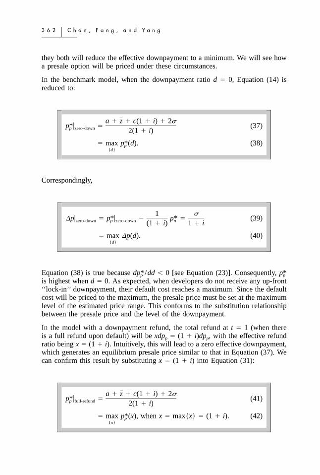
they both will reduce the effective downpayment to a minimum. We will see howa presale option will be priced under these circumstances.

In the benchmark model, when the downpayment ratio d � 0, Equation (14) isreduced to:

a � z � c(1 � i) � 2�p*� � (37)p zero-down 2(1 � i)

� max p*(d). (38)p{d}

Correspondingly,

1 ��p� � p*� � p* � (39)zero-down p zero-down n(1 � i) 1 � i

� max �p(d). (40){d}

Equation (38) is true because /dd � 0 [see Equation (23)]. Consequently,dp* p*p p

is highest when d � 0. As expected, when developers do not receive any up-front‘‘lock-in’’ downpayment, their default cost reaches a maximum. Since the defaultcost will be priced to the maximum, the presale price must be set at the maximumlevel of the estimated price range. This conforms to the substitution relationshipbetween the presale price and the level of the downpayment.

In the model with a downpayment refund, the total refund at t � 1 (when thereis a full refund upon default) will be xdpp � (1 � i)dpp, with the effective refundratio being x � (1 � i). Intuitively, this will lead to a zero effective downpayment,which generates an equilibrium presale price similar to that in Equation (37). Wecan confirm this result by substituting x � (1 � i) into Equation (31):

a � z � c(1 � i) � 2�p*� � (41)p full-refund 2(1 � i)

� max p*(x), when x � max{x} � (1 � i). (42)p{x}

P r e s a l e s , F i n a n c i n g C o n s t r a i n t s , a n d D e v e l o p e r s ’ � 3 6 3

J R E R � V o l . 3 0 � N o . 3 – 2 0 0 8

Correspondingly,

1 ��p� � p*� � p* � (43)full-refund p full-refund n(1 � i) 1 � i

� max �p(x). (44){x}

Equation (42) holds because /dx � 0 [see Equation (34)]. Consequently,dp* p*p p

is highest when x � max{x} � (1 � i). These two special cases furtherdemonstrate a commonly known principle that there is no free lunch. A lessstringent downpayment (with refund) policy must end up with a less favorablecontract price. A more favorable contract price must be accompanied by a tougherdownpayment policy.6

At this moment, our model implicitly assumes that the presale method doesnot affect a developer’s production decision (and hence, the market structure).However, it is possible that, when there is a financing constraint on a developer’sequity side, the developer’s production decision will be affected. This is the casebecause there is a cost saving if the developer can receive a downpayment beforethe project starts. This issue is examined in the next section.

� F i n a n c i n g C o n s t r a i n t s

We now consider that the function of a presale is to help developers raise equityfor their developments. In Asia, where debt financing is hard to get, it is commonknowledge that the motivation for developers to employ the presale method is toraise equity capital. In the benchmark model, we ignore this possibility and assumethat a developer can finance the development with his own equity or with debt ifit can be obtained at a reasonable cost.

In the real world, developers have to raise debt to finance their developments. Itshould be noted that, in many Asian countries, the financing cost could be highbecause of the tight capital markets. More importantly, debt financing might notbe available at all to developers who do not have adequate equity capital. Inaddition, the cost of debt, if debt is available, is a function of the amount of equityin the project. With a presale, a developer can receive the downpayments of presalecontracts before project construction starts. This cash infusion will help increasethe developer’s equity contribution and, hence, reduce his debt financing cost. Onthe other hand, if we keep the leverage ratio constant and use the downpaymentas equity, a developer can increase the size of his development project.

3 6 4 � C h a n , F a n g , a n d Y a n g

We now revise our benchmark model to take into account financing constraints.We define the total development cost as cq. If we assume that the developer’sonly equity source to finance the development is the buyer’s downpayment, thencdq is financed with equity. The rest of the development cost will be financedwith debt at an interest rate r. The cost of debt is c(1 � d)(1 � r)q. We assumer � r0 � wd, where r0 is the baseline interest rate and w is the sensitivity ofinterest rate reduction to the presale downpayment ratio (or the leverage ratio).This means that, the higher the equity level, the lower the interest rate will be forthe development project. The developer’s development cost can be rewritten as:

cdq � c(1 � d)(1 � r)q � c[d � (1 � d)(1 � r � wd)]q.0 (45)

Note that if we set w � 0 and r0 � 0 (i.e., debt is interest free), the cost functionwill collapse to that used in the benchmark model.

It is clear that the development-cost reduction affects a developer’s production andpricing decisions, but not the buyer’s decision. With backward induction, thebuyer’s decision rules are the same as before. At t � 1, she will choose to continuewith the presale payment if:

z � z � �a � bq � (1 � d)(1 � i)p ; (46)p

At t � 0, she will accept the presale offer if:

a � z � bqp � p (q) �p p (1 � d)(1 � i)

(1 � d)� � 2d�[� � (1 � d)(a � z � bq)]� .2(1 � d) (1 � i)

(47)

However, the developer’s optimization problem for offering an acceptable presalesdeal is now changed to:

P r e s a l e s , F i n a n c i n g C o n s t r a i n t s , a n d D e v e l o p e r s ’ � 3 6 5

J R E R � V o l . 3 0 � N o . 3 – 2 0 0 8

z��

E(�)� � max � p qd�(z)presale pz{p ,q}p

z 1� � [dp q � (a � z � bq)q]d�(z)p

z�� (1 � i)

�c[d � (1 � d)(1 � r � wd)]q � K,0

where

z � �a � bq � (1 � d)(1 � i)p ,p

a � z � bqs.t. p � p (q) �p p (1 � d)(1 � i)

(1 � d)� � 2d�[� � (1 � d)(a � z � bq)]� .2(1 � d) (1 � i)

(48)

Note that the marginal development cost c in the benchmark model changes to c[d � (1 � d)(1 � r0 � wd)]. The developer’s optimization problem under a spotsale is similar to the process we used in the benchmark model, except that nowwe also consider financing constraints, or:

z�� 1E(�)� � max � p q � c(1 � r )q d�(z), (49)� �spot n n 0 n

z�� (1 � i){q }n

where p � a � z � bq .n n

The equilibrium outcomes of the case are presented in Proposition 2.

Proposition 2. In equilibrium, the optimal price and optimal quantity of a presalecontract (with financing constraints) are:

a � z � c(1 � i)q* � , (50)p 2b

a � z � c(1 � i)p* �p 2(1 � d)(1 � i)

�(1 � d) �2d�[(1 � d)(a � z � c(1 � i)) � 2�]

� , (51)2(1 � d) (1 � i)

where � d � (1 � d)(1 � r � wd).0

3 6 6 � C h a n , F a n g , a n d Y a n g

The optimal price and optimal quantity of a spot sale contract are:

a � z � c(1 � r )(1 � i)0q* � , (52)n 2b

a � z � c(1 � r )(1 � i)0p* � . (53)n 2

The development scale is greater under a presale contract, with:

q* � q*. (54)p n

Ignoring the presale-specific transaction cost K, a developer is better off offeringa presale contract than a spot sale contract, with:

E(�(p*, q*))� � E(�(p*, q*))� . (55)p p presale n n spot

A buyer’s expected cost of buying the property is also lower under a presalecontract than a spot sale, with:

E(C(p*, q*))� � E(C(p*, q*))� � E(C(p*, q*))� .p p accept p p decline n n spot (56)

Finally, the development scale and a developer’s profit are positively affected bythe sensitivity of the debt cost to the leverage ratio (w), while a buyer’s expectedcost is negatively related to w, or:

d�q d�E(�) d�E(C)� 0, � 0 and � 0. (57)

dw dw dw

Proof. See Appendix B. �

Proposition 2 highlights the importance of the presale method in a market withfinancing constraints. With a presale method, a developer is able to obtain cashbefore a project actually starts. The cash inflows associated with the downpaymentof a presale contract can be used by developers as the equity for the development.Since developers have more equity with a presale method, it is easier for them

P r e s a l e s , F i n a n c i n g C o n s t r a i n t s , a n d D e v e l o p e r s ’ � 3 6 7

J R E R � V o l . 3 0 � N o . 3 – 2 0 0 8

to obtain debt financing at a lower interest rate. This reduces the marginaldevelopment cost of the project. Under this circumstance, the developer enjoysadditional cost savings when compared with the use of the spot sale method. Whenthe developer shares the savings with the buyer, the buyer can buy the propertyat a price lower than if there were no presale contract. Therefore, both thedeveloper and the buyer are better off with the presale method. This is probablywhy the presale method is more popular in those Asian countries with lessdeveloped financial systems.

It is important to note that this cost-saving efficiency can also result in a largerdevelopment scale. Holding the leverage ratio of a development constant, the cashinflow obtained from the presale method allows a developer to increase thedevelopment size. This means that we will observe more developments in a marketin which the presale method is used than in one that only allows spot sales. Giventhis, in property markets with tight capital constraints (such as in China) wherethe underlying motivation for employing the presale method is to overcomefinancing constraints, we should observe aggressive development patterns. Thisseems to be the phenomenon we have been observing in these markets in recentyears.

� C o n c l u s i o n

The presale method has frequently been used in property markets all over theworld, particularly in Asia. However, even with more than five decades ofexperience with this system, we still do not know much about its impact onproperty markets, except that developers can use the method to share thedevelopment risk with buyers (see Lai, Wang, and Zhou, 2004).

In this paper, we develop a model to explore the impacts of the presale methodon a developer’s pricing and production decisions. We find that the presale methoditself does not affect a developer’s production decision, nor the welfare of a buyerwhen there are no financing constraints in the market. In an efficient market,developers will simply adjust the presale price to account for the option valuethey give to buyers in the presale market and, as such, both developers and buyersare indifferent between a presale method and a spot sale method.

However, in a market with a nascent financial system where debt financing maynot be available to developers at a reasonable cost, the presale system is beneficialto both developers and buyers. This is the case because the downpayment from apresale contract can be used as equity for a development. Under this scenario, weshow that developers will pursue aggressive development strategies. This resultseems to be consistent with the aggressive building behaviors of developers insome of the Asian real estate markets.

The popular press also mentions that the most important reason for the existenceof the presale system is buyers’ belief that if they do not buy now, they will notbe able to buy in the future. In other words, the ‘‘last bus’’ fear drives buyers to

3 6 8 � C h a n , F a n g , a n d Y a n g

the presale market. While this argument makes some sense, it is difficult to modelit under a rational framework.7 However, it may be worthwhile for future researchon the presale system to address this kind of behavioral argument.

� A p p e n d i x�� A . P r o o f f o r P r o p o s i t i o n 1

Our first attempt is to simultaneously solve for the optimal and q. Thep*pdecomposition of Equation (9) with K � 0 generates:

1E(�)� �presale 4(1 � i)z

2 3 2(A p � A p � B q � B q � B q � C), (58)1 p 2 p 1 2 3

2 2where A � �(1 � d) (1 � i) q � 0,1

2B � �b � 0, and A , B , B and C2 2 3

are the combinations of parameters.

The unconstrained optimum p0 is derived from a first-order condition:

dE(�)�presale o� 0 ⇒ p* � pp 0dp0

(1 � d)(a � z � bq) � (1 � d)�� , (59)2(1 � i)(1 � d)

and this result must maximize the expected profit since the second-order conditionsatisfies:

2 2d E(�)� (1 � d) (1 � i)qpresale � � � 0. (60)2dp 2z0

P r e s a l e s , F i n a n c i n g C o n s t r a i n t s , a n d D e v e l o p e r s ’ � 3 6 9

J R E R � V o l . 3 0 � N o . 3 – 2 0 0 8

However, comparing with defined in Equation (8), we find:op p (q)0 p

2d�[� � (1 � d)(a � z � bq)]op � p (q) � � 0. (61)0 p 2(1 � d) (1 � i)

Since the unconstrained optimum exceeds the upper boundary constraintop0

this unconstrained optimum cannot be a feasible solution for the problem.p (q),p

Given the observation that E(�)�presale is a concave function of pp, we know thatthe optimum should be the constrained maximum level of pp. Consequently:p*p

a � z � bqp* � p (q) �p p (1 � d)(1 � i)

(1 � d)� � 2d�[� � (1 � d)(a � z � bq)]� . (62)2(1 � d) (1 � i)

The optimum q, however, cannot be solved since E(�)�presale is a cube function ofq and the multiplier for term q3 is negative. (Under this circumstance, we can onlyfind a local minimum, but not any local or global maximum.)

We hence try to solve for the sequential optima starting from q to Withp*.p

backward induction, we derive the optimum first. Following steps similar top*pthose mentioned above, we derive the optimum as shown in Equation (62).p*pThen we solve for the optimal q by incorporating optimal into the expectedp*ppayoff function, resulting in:

a � z � bqE(�(p*(q), q))� � q � c � K. (63)� �p presale 1 � i

The optimum q is then derived from a first-order condition:

dE(�(p*(q), q))� a � z � c(1 � i)p presale� 0 ⇒ q � q* � , (64)

dq 2b

and this result must maximize the expected profit since the second-order conditionsatisfies:

3 7 0 � C h a n , F a n g , a n d Y a n g

2d E(�(p*(q), q))� 2bp presale� � � 0. (65)2dq (1 � i)

Substituting q* into Equation (62), we derive the optimal presale price as:

a � z � c(1 � i)p* �p 2(1 � d)(1 � i)

�(1 � d) � 2d�[(1 � d)(a � z � c(1 � i)) � 2�]� .2(1 � d) (1 � i)

(66)

From the optimization problem under the spot sale [in Equation (10)], it is easyto derive that the optimal spot sale price and quantity are:

a � z � c(1 � i)q* � , and (67)n 2b

a � z � c(1 � i)p* � . (68)n 2

Finally, we substitute q* and into Equations (5), (6), and (9), and andp* q* p*p n n

into Equations (10) and (11). We find that when the presale-specific transactioncost K � 0:

E(�(p*, q*))� � E(�(p*, q*))�p p presale n n spot

2[a � z � c(1 � i)]� . (69)

4b(1 � i)

That is, the developer is indifferent between offering a presale and offering a spotsale. In addition, since:

P r e s a l e s , F i n a n c i n g C o n s t r a i n t s , a n d D e v e l o p e r s ’ � 3 7 1

J R E R � V o l . 3 0 � N o . 3 – 2 0 0 8

E(C(p*, q*))� � E(C(p*, q*))�p p accept p p decline

a � z � c(1 � i)� E(C(p*, q*))� � , (70)n n spot 2(1 � i)

it suggests that a buyer’s expected cost of buying the property is the sameregardless of the selling method used by the developer. � Q.E.D.

� B . P r o o f f o r P r o p o s i t i o n 2

To solve this problem, we use a procedure similar to the one used to solve forthe equilibrium solution for the benchmark model. With financing constraints anda possible development cost reduction, we solve the optimization problem asdetailed in Equation (48). Clearly, the equilibrium presale quantity and price are:

a � z � c(1 � i)q* � , (71)p 2b

a � z � c(1 � i)p* �p 2(1 � d)(1 � i)

�(1 � d)�2d�[(1 � d)(a � z � c(1 � i)) � 2�]

� , (72)2(1 � d) (1 � i)

where � d � (1 � d)(1 � r � wd).0

The developer’s expected profits and the buyer’s expected cost under a presalecontract are now changed to:

2[a � z � c(1 � i)]E(�(p*, q*))� � � K, (73)p p presale 4b(1 � i)

E(C(p*, q*))� � E(C(p*, q*))�p p accept p p decline

a � z � c(1 � i)� . (74)

2(1 � i)

By solving the optimization problem in Equation (49), we can derive that, withfinancing constraints, the equilibrium spot sale quantity and spot sale price are:

3 7 2 � C h a n , F a n g , a n d Y a n g

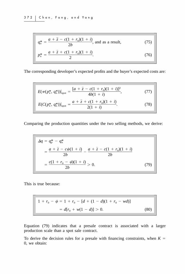
a � z � c(1 � r )(1 � i)0q* � , and as a result, (75)n 2b

a � z � c(1 � r )(1 � i)0p* � . (76)n 2

The corresponding developer’s expected profits and the buyer’s expected costs are:

2[a � z � c(1 � r )(1 � i)]0E(�(p*, q*))� � , (77)n n spot 4b(1 � i)

a � z � c(1 � r )(1 � i)0E(C(p*, q*))� � . (78)n n spot 2(1 � i)

Comparing the production quantities under the two selling methods, we derive:

�q � q* � q*p n

a � z � c(1 � i) a � z � c(1 � r )(1 � i)0� �2b 2b

c(1 � r � )(1 � i)0� � 0. (79)2b

This is true because:

1 � r � � 1 � r � [d � (1 � d)(1 � r � wd)]0 0 0

� d[r � w(1 � d)] � 0. (80)0

Equation (79) indicates that a presale contract is associated with a largerproduction scale than a spot sale contract.

To derive the decision rules for a presale with financing constraints, when K �0, we obtain:

P r e s a l e s , F i n a n c i n g C o n s t r a i n t s , a n d D e v e l o p e r s ’ � 3 7 3

J R E R � V o l . 3 0 � N o . 3 – 2 0 0 8

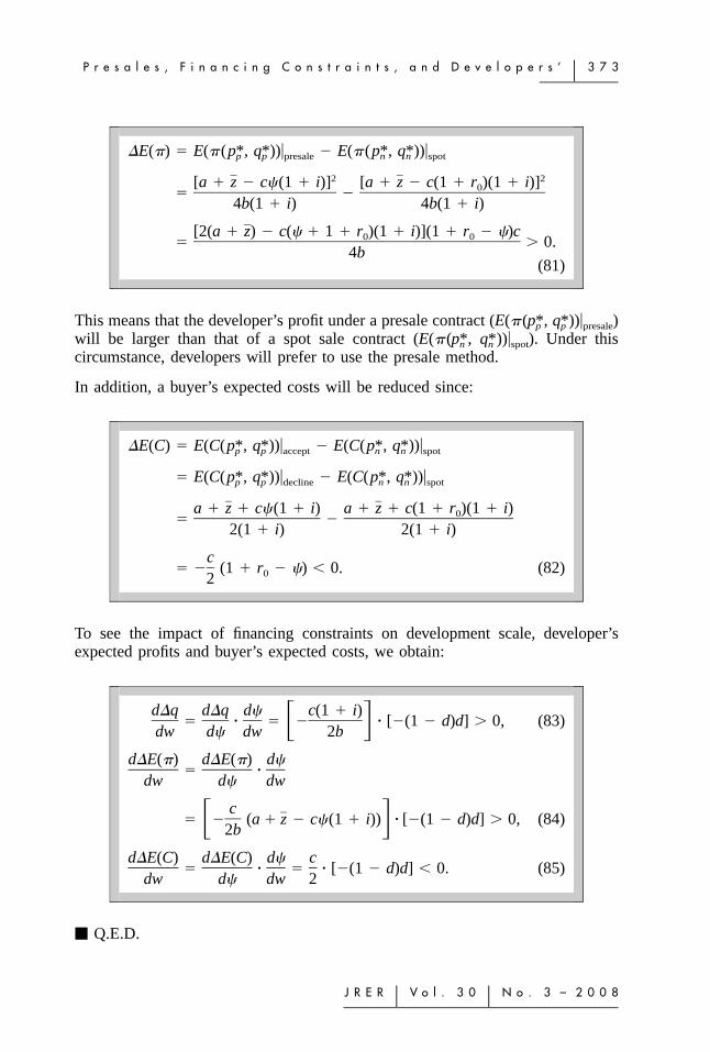
�E(�) � E(�(p*, q*))� � E(�(p*, q*))�p p presale n n spot

2 2[a � z � c(1 � i)] [a � z � c(1 � r )(1 � i)]0� �4b(1 � i) 4b(1 � i)

[2(a � z) � c( � 1 � r )(1 � i)](1 � r � )c0 0� � 0.4b

(81)

This means that the developer’s profit under a presale contract (E(�( ))�presale)p*, q*p p

will be larger than that of a spot sale contract (E(�( ))�spot). Under thisp*, q*n n

circumstance, developers will prefer to use the presale method.

In addition, a buyer’s expected costs will be reduced since:

�E(C) � E(C(p*, q*))� � E(C(p*, q*))�p p accept n n spot

� E(C(p*, q*))� � E(C(p*, q*))�p p decline n n spot

a � z � c(1 � i) a � z � c(1 � r )(1 � i)0� �2(1 � i) 2(1 � i)

c� � (1 � r � ) � 0. (82)02

To see the impact of financing constraints on development scale, developer’sexpected profits and buyer’s expected costs, we obtain:

d�q d�q d c(1 � i)� � � � � [�(1 � d)d] � 0, (83)� �dw d dw 2b

d�E(�) d�E(�) d� �

dw d dw

c� � (a � z � c(1 � i)) � [�(1 � d)d] � 0, (84)� �2b

d�E(C) d�E(C) d c� � � � [�(1 � d)d] � 0. (85)

dw d dw 2

� Q.E.D.

3 7 4 � C h a n , F a n g , a n d Y a n g

� E n d n o t e s1 See Chang and Ward (1993), Wang, Zhou, Chan, and Chau (2000), Hua, Chang, and

Hsieh (2001), Lai, Wang, and Zhou (2004), and Wong, Yiu, Tse, and Chau (2006) for adiscussion of the presale method. The presale method has been used in many cities aroundthe world, but is particularly popular in several Asian countries/regions, such as HongKong, Taiwan, Korea, Singapore, and Mainland China.

2 See the August 22, 2006 Los Angeles Times article titled ‘‘State 2nd in Housing Growth,Census Data Say.’’

3 This seems especially odd given that Asian researchers and institutions have significantlyincreased their influence in top-tier real estate publications, according to an assessmentby Chan, Hardin, Liano, and Yu (2008) of the 1990–2006 real estate literature.

4 Wang and Zhou (2000), among others, also used a game-theoretical approach to modelthe over-building phenomenon in real estate markets.

5 The option concept has been applied to the study of many issues in real estate markets.See, for example, Grenadier (1995, 1996), Buetow and Albert (1998), Harrison,Noordewier, and Ramagopal (2002), Clapham (2003), Lai, Wang, and Zhou (2004),Svenstrup and Willemann (2006), Wang and Zhou (2006), and Lai, Wang, and Yang(2007).

6 The downpayment issues have been examined by Stein (1995) and Leung, Lau, andLeong (2002). Both papers discuss the downpayment effect in the formation of a positiverelation between property prices and trading volume.

7 Wang, Young, and Zhou (2002) successfully used a rational model to explain a seeminglyirrational phenomenon (banks foreclosing on properties without negotiations) in themarket. Given this, it might be possible to find a rational model to explain this momentumbuying (or ‘‘last bus’’) phenomenon.

� R e f e r e n c e s

Buetow, G. and J. Albert. The Pricing of Embedded Options in Real Estate Lease Contracts.Journal of Real Estate Research, 1998, 15:3, 253–65.

Chan, K.C., W.G. Hardin III, K. Liano, and Z. Yu. The Internationalization of Real EstateResearch. Journal of Real Estate Research, 2008, 30:1, 91–124.

Chang, C.O. and C.W. Ward. Forward Pricing and the Housing Market: The Pre-SalesHousing System in Taiwan. Journal of Property Research, 1993, 10, 217–27.

Clapham, E. A Note on Embedded Lease Options. Journal of Real Estate Research, 2003,25:3, 347–59.

Grenadier, S.R. Valuing Lease Contracts: A Real-Option Approach. Journal of FinancialEconomics, 1995, 38, 297–331.

——. The Strategic Exercise of Options: Development Cascades and Overbuilding in RealEstate. Journal of Finance, 1996, 51, 1653–79.

Harrison, D.M., T.G. Noordewier, and K. Ramagopal. Mortgage Terminations: The Roleof Conditional Volatility. Journal of Real Estate Research, 2002, 23, 89–110.

Hua, C.C., C.O. Chang, and C. Hsieh. The Price-Volume Relationships between theExisting and the Pre-Sales Housing Markets in Taiwan. International Real Estate Review,2001, 4:1, 80–94.

P r e s a l e s , F i n a n c i n g C o n s t r a i n t s , a n d D e v e l o p e r s ’ � 3 7 5

J R E R � V o l . 3 0 � N o . 3 – 2 0 0 8

Lai, R.N., K. Wang, and J. Yang. Stickiness of Rental Rates and Developers’ OptionExercise Strategies. Journal of Real Estate Finance and Economics, 2007, 34:1, 159–88.

Lai, R.N., K. Wang, and Y. Zhou. Sale before Completion of Development: Pricing andStrategy. Real Estate Economics, 2004, 32:2, 329–57.

Leung, C., G. Lau, and Y. Leong. Testing Alternative Theories of the Property Price-tradingVolume Correlation. Journal of Real Estate Research, 2002, 23:3, 253–63.

Stein, J. Prices and Trading Volume in the Housing Market: A Model with DownpaymentEffects. Quarterly Journal of Economics, 1995, 110, 379–405.

Svenstrup, M. and S. Willemann. Reforming Housing Finance: Perspectives from Denmark.Journal of Real Estate Research, 2006, 28:2, 105–29.

Wang, K., L. Young, and Y. Zhou. Non-discriminating Foreclosure and VoluntaryLiquidating Costs. Review of Financial Studies, 2002, 15:3, 959–85.

Wang, K. and Y. Zhou. Overbuilding: A Game-Theoretic Approach. Real Estate Economics,2000, 28:3, 493–522.

Wang, K. and Y. Zhou. Equilibrium Real Options Exercise Strategies with Multiple Players:The Case of Real Estate Markets. Real Estate Economics, 2006, 34:1, 1–49.

Wang, K., Y. Zhou, S.H. Chan, and K.W. Chau. Over-Confidence and Cycles in Real EstateMarkets: Cases in Hong Kong and Asia. International Real Estate Review, 2000, 3:1, 93–108.

Wong, S.K., C.Y. Yiu, M.K.S. Tse, and K.W. Chau. Do the Forward Sales of Real EstateStabilize Spot Prices? Journal of Real Estate Finance and Economics, 2006, 32, 289–304.

We acknowledge helpful comments from Rose Lai, David Barker, participants at the12th AsRES Annual Conference, and the referees of this journal.

Su Han Chan, California State University–Fullerton, Fullerton, CA 92834 orschan@fullerton.edu.

Fang Fang, Shanghai University of Finance and Economics, Shanghai, P.R. China,200433 or ffang@mail.shufe.edu.cn.

Jing Yang, California State University–Fullerton, Fullerton, CA 92834 orjyang@fullerton.edu.