Preprocessing of airborne pyranometer data.
45
NCAR/TN-364+STR NCAR TECHNICAL NOTE September 1991 Preprocessing of Airborne Pyranometer Data Lutz Bannehr Advanced Study Program of the Office of the Director, and Research Aviation Facility of the Atmospheric Technology Division National Center for Atmospheric Research, Boulder, CO 80307-3000 Vince Glover Research Aviation Facility of the Atmospheric Technology Division National Center for Atmospheric Research, Boulder, CO 80307-3000 RESEARCH AVIATION FACILITY ATMOSPHERIC TECHNOLOGY DIVISION NATIONAL CENTER FOR ATMOSPHERIC RESEARCH BOULDER, COLORADO I - LI _ _ I -- I -~~~~~~~~~~~~~~ I - ~ ~~ ~ ~~~~~~~ ~ ~ ~ ~ ~ ~ ~~~~~~~~~~~~~~~ II-· I· I I
Transcript of Preprocessing of airborne pyranometer data.
NCAR/TN-364+STRNCAR TECHNICAL NOTE
September 1991
Preprocessing of AirbornePyranometer Data
Lutz BannehrAdvanced Study Program of the Office of the Director, andResearch Aviation Facility of the Atmospheric Technology DivisionNational Center for Atmospheric Research, Boulder, CO 80307-3000
Vince GloverResearch Aviation Facility of the Atmospheric Technology DivisionNational Center for Atmospheric Research, Boulder, CO 80307-3000
RESEARCH AVIATION FACILITYATMOSPHERIC TECHNOLOGY DIVISION
NATIONAL CENTER FOR ATMOSPHERIC RESEARCHBOULDER, COLORADO
I - LI _ _ I - - I -~~~~~~~~~~~~~~I
- ~ ~~ ~ ~~~~~~~ ~ ~ ~ ~ ~ ~ ~~~~~~~~~~~~~~~ II-· I· I I
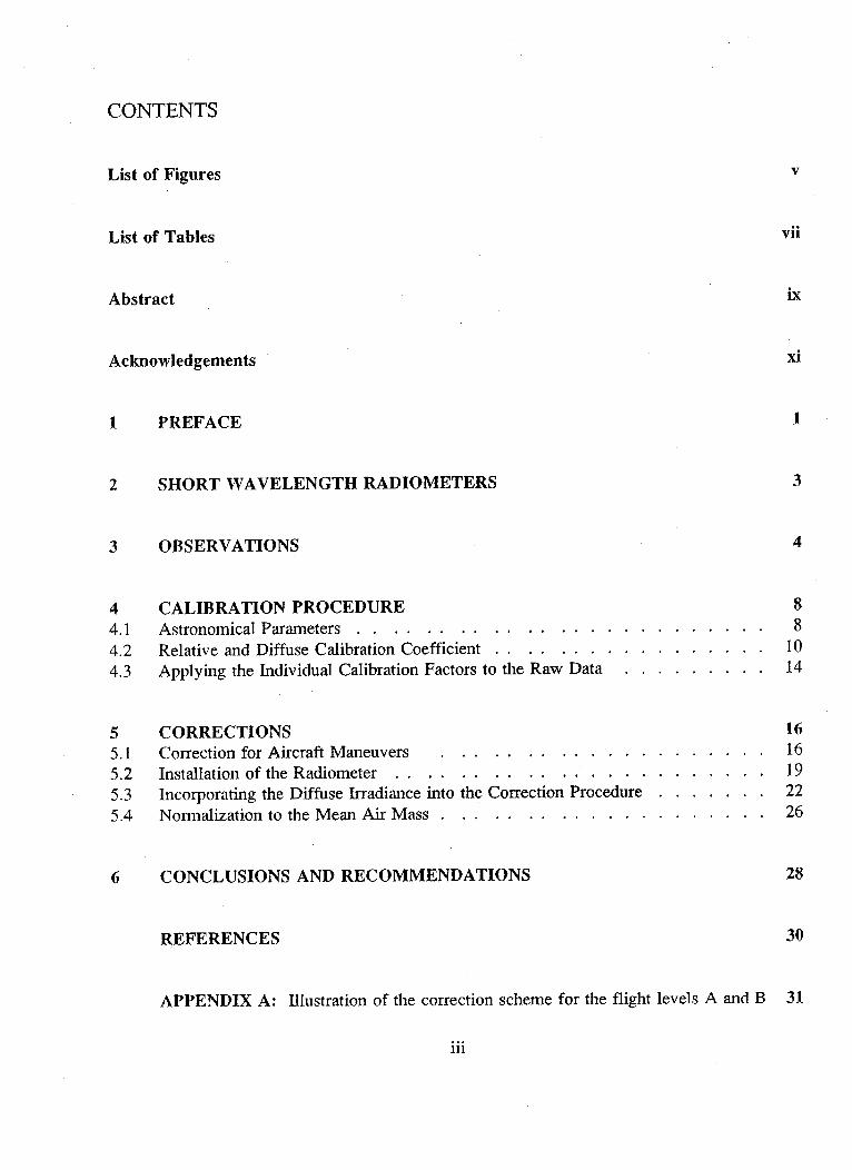
CONTENTS
List of Figures v
List of Tables vii
Abstract ix
Acknowledgements xi
1 PREFACE1
2 SHORT WAVELENGTH RADIOMETERS 3
3 OBSERVATIONS 4
4 CALIBRATION PROCEDURE 84.1 Astronomical Parameters. .............. 8
4.2 Relative and Diffuse Calibration Coefficient ................. 104.3 Applying the Individual Calibration Factors to the Raw Data . . . . . . . . . 14
5 CORRECTIONS 165.1 Correction for Aircraft Maneuvers . ................... 165.2 Installation of the Radiometer ... . . . . . . . . . . . 19
5.3 Incorporating the Diffuse Irradiance into the Correction Procedure . . . . . . . 22
5.4 Normalization to the Mean Air Mass ................... 26
6 CONCLUSIONS AND RECOMMENDATIONS 28
REFERENCES 30
APPENDIX A: Illustration of the correction scheme for the flight levels A and B 31
iii


LIST OF FIGURES
PAGE
43.1 Sketch of the flight pattern. The linear connections between the letters A, Band C denote the traverse sections (at three different levels designated A,Band C in the text) which were analyzed.
3.2 Unprocessed global irradiance data together with the pitch and roll anglesof the aircraft.
4.1 Relative calibration factor of the upward facing pyranometer.
4.2 Diffuse calibration coefficient for different anisotropy parameters b for theupward facing radiometer.
5.1 Illustration of the correction scheme for flight level C.
5.2 Pitch and roll variations during the observations at flight level C (216.7 hPa).
5.3 Comparison of misalignments of the upward looking pyranometer (traverse B).
5.4a Simulated ratio of diffuse to direct irradiance for different solaraltitudes and high loading of atmospheric constituents.
5.4b Simulated ratio of diffuse to direct irradiance for different solaraltitudes and low loading of atmospheric constituents.
v
5
12
14
17
18
21
23
24

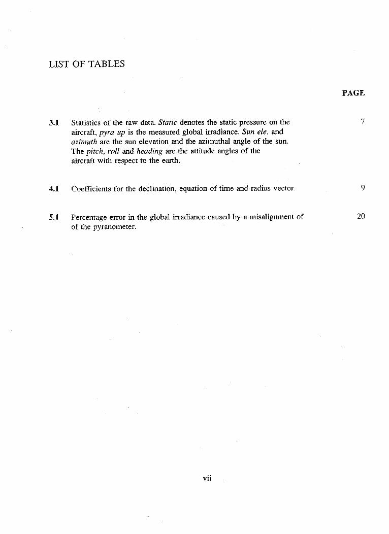
LIST OF TABLES
PAGE
73.1 Statistics of the raw data. Static denotes the static pressure on theaircraft, pyra up is the measured global irradiance. Sun ele. andazimuth are the sun elevation and the azimuthal angle of the sun.The pitch, roll and heading are the attitude angles of theaircraft with respect to the earth.
4.1 Coefficients for the declination, equation of time and radius vector.
5.1 Percentage error in the global irradiance caused by a misalignment ofof the pyranometer.
vii
9
20


ABSTRACT
On the three research aircraft of the National Center for Atmospheric Research (NCAR),
Eppley pyranometers are employed to measure the up- and downwelling short wavelength
radiation fluxes in the atmosphere. The quality of the data used to investigate the radiation
budget and extinction of solar irradiance depends strongly on the calibration and correction
applied to the radiation data, accounting for (1) cosine response of the instruments, (2) ambient
temperature effects, (3) leveling of the radiometers, and (4) aircraft maneuvers during the
observations. This report makes suggestions about how the quality of the radiation data can be
enhanced by a more accurate calibration procedure and correction scheme. By considering the
recommnendations, data from the upward facing pyranometer can be improved by about 20%
*under clear sky conditions.
In order to improve the pyranometer data under cloudy conditions by the same percentage,
the diffuse irradiance must be measured in addition to the global irradiance.
ix

ACKNOWLEDGEMENTS
The authors wish to express their appreciation to the many people who contributed to and
supported this work. John DeLuisi and Donald Nelson of the Climate Monitoring and
Diagnostics Laboratory, NOAA/ERL/CMDL, made it possible to obtain a high quality calibration
of the pyranometer used in this study. John DeLuisi made the calibration facilities available and
Donald Nelson performed the calibration. Ronald Smith of Yale University generously provided
the data set, SMT1 1, used for verifying the methods developed in this Tech Note. The satellite
images used to verify the presence of clouds at the time and place of the SMT1 1 observations
were obtained through the research efforts of John Brown of the Forecast Systems Laboratory,
NOAA/ERL. Special thanks are due to Dave McFarland of the NCAR Research Aviation
Facility (RAF). He consulted with us numerous times on the characteristics of pyranometers and
other radiation instruments. Ronald Schwiesow and Darrel Baumgardner of the RAF reviewed
the draft of the technical note and made valuable suggestions on improving the quality of the
work.
This research has been supported by the National Science Foundation.
Lutz Bannehr
September 1991
xi

1 PREFACE
In recent years, concern about the impact of human activity on our climate has grown
considerably. Accurate data on parameters such as net short wave and long wave radiation,
heating rate, and absorption and scattering by the atmospheric constituents are needed to provide
input data for general circulation models. Airborne investigations are undertaken in order to
study the radiation budget and extinction of incoming solar irradiance by using UV-radiometers,
pyranometers and pyrgeometers. However, operating such radiometers on research airplanes to
obtain high quality data is not a simple task, because these instruments are designed for ground-
based operations. Their performance suffers drastically when used on aircraft due to extreme
atmospheric conditions as well as aircraft maneuvers. Therefore, the results of the measurements
and the conclusions drawn from them are very dependent on the quality of the data used.
Reliable values for the flux divergence derived from airborne radiation measurements can only
be obtained by performing calibrations and corrections carefully so that uncertainties are
minimized.
For calibration, the pyranometers are sent to the manufacturer, Eppley Laboratories. One
calibration coefficient is given for all zenith angles. By considering the cosine response of the
pyranometers, the accuracy of the global and reflected radiation data can be slightly enhanced.
Applying corrections to the upward facing pyranometer to compensate for the inclination of the
instrument during airborne observations improved the data by almost 12% as will be
demonstrated in Section 5.1. This correction is the main contribution to reducing uncertainty.
Another important factor, especially if the investigations are carried out at low solar altitude, is
that the pyranometer should be aligned as closely as possible with the aircraft inertial navigation
system. Radiative transfer calculations indicated that a misalignment of ±2° can cause an error
of about ±9% at a sun elevation of 25°.
In this report, the global irradiance data of flight SMTll, performed on January 19, 1989,
will be analyzed. It will be shown how the accuracy of the shortwave radiation data can be
1

improved when the necessary calibrations are performed and corrections are applied to thecollected data. The correction procedure for the reflected radiation data is not as critical as for
the global irradiance data. Hence, rather then analyzing the time series of the upwelling radiation
data in detail, only some comments will be made on how they can be improved.
Future work is required to enhance the quality of the radiometer data further. The
development of a shading device to measure the diffuse irradiance from aircraft in addition tothe global irradiance is essential in order to correct the data properly. Also, more development
effort is necessary in order to correct pyranometers for temperature sensitivity as is done withpyrgeometers.
2
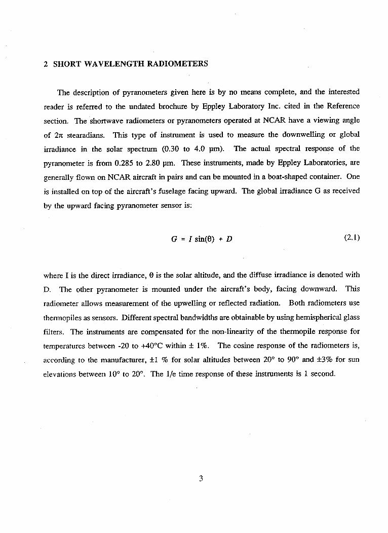
2 SHORT WAVELENGTH RADIOMETERS
The description of pyranometers given here is by no means complete, and the interested
reader is referred to the undated brochure by Eppley Laboratory Inc. cited in the Reference
section. The shortwave radiometers or pyranometers operated at NCAR have a viewing angle
of 2I stearadians. This type of instrument is used to measure the downwelling or global
irradiance in the solar spectrum (0.30 to 4.0 pm). The actual spectral response of the
pyranometer is from 0.285 to 2.80 pm. These instruments, made by Eppley Laboratories, are
generally flown on NCAR aircraft in pairs and can be mounted in a boat-shaped container. One
is installed on top of the aircraft's fuselage facing upward. The global irradiance G as received
by the upward facing pyranometer sensor is:
G = I sin(O) + D (2.1)
where I is the direct irradiance, 0 is the solar altitude, and the diffuse irradiance is denoted with
D. The other pyranometer is mounted under the aircraft's body, facing downward. This
radiometer allows measurement of the upwelling or reflected radiation. Both radiometers use
thermopiles as sensors. Different spectral bandwidths are obtainable by using hemispherical glass
filters. The instruments are compensated for the non-linearity of the thermopile response for
temperatures between -20 to +40°C within ± 1%. The cosine response of the radiometers is,
according to the manufacturer, ±1 % for solar altitudes between 20° to 90° and ±3% for sun
elevations between 10° to 20°. The l/e time response of these instruments is 1 second.
3
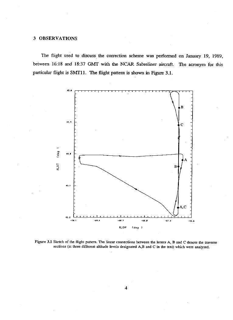
3 OBSERVATIONS
The flight used to discuss the correction scheme was performed on January 19, 1989,
between 16:18 and 18:37 GMT with the NCAR Sabreliner aircraft. The acronym for this
particular flight is SMTll. The flight pattern is shown in Figure 3.1.
45.8
44.9
0)* 44.1
4:.
-
43.1
42.2
-70.1 -69.4 -68.7 -68.0 -67.3 -66.6
ALON (deg )
Figure 3.1 Sketch of the flight pattern. The linear connections between the letters A, B and C denote the traversesections (at three different altitude levels designated AB and C in the text) which were analyzed.
4

Figure 3.2 shows the time series of the global irradiance, the pitch angle and roll angle of
the aircraft during the observation of the SMT1 1 flight. The data were collected at a rate of 50
Flight SMT11 -1/19/89-800
700CM
I
IE
600uc
4C-'= 500
s-L.c.
- 400
0-D
300
200
6
4
: 2IL1
0
cr0
-2
-4
0 1000 2000 3000 4000 5000 6000
Samples
Figure 3.2 Unprocessed global irradiance data together with the roll and pitch angles of the aircraft.
5
v I i1 M vI 1 AA a Mvy kV Y I
\v
8
I10
6
a-
2
07000
I » » . . i . I I I . I . ...... !s I.......IIV V II
. . . . .. . . . . . . . . . . . . .A.I
1
d a
. . . . . . . .I . . q I I I I I . . g . . . . . . . . .
i
II I MIA. AAlk AA

Hz and averaged over one second. One second is equivalent to one sample in Figure 3.2. The
strong influence of pitch and roll movements on the global irradiance can be clearly seen. In
situations where the pitch and roll angles are large, the instrument senses not only the
downwelling radiation but also receives a large proportion of the upwelling radiation. Since it
is not possible to distinguish clearly between the two different signals, no correction can be
applied to the radiation data and the data are rejected for further processing. Hence, the analyzed
observations are divided into several sections. The criterion for the current analyses is that the
radiometric data are excluded where the pitch or roll angles exceed ±6°. Therefore, runs without
ascents, descents, or turns are used for the processing. To circumvent the problem of differential
heating of the pyranometer, which causes an error in the output signal, only data 20 seconds after
reaching the cruising altitude are chosen. The values selected are divided in the three consecutive
levels A, B and C at mean pressure levels of 315.25, 238.81 and 216.74 hPa. Due to the nature
of the flight operations and the constraints on the aircraft attitude, given above, each processed
time series has a different length. The selected data for level A are between samples 1600 and
2350, for level B between 3250 and 4100, and for level C between 4900 and 6200. Some basic
flight statistics of the SMT1 1 are given in Table 3.1, such as the average value, MEAN, for each
level, the minimum, MIN, and maximum, MAX, as well as the standard deviation, SDEV.
6
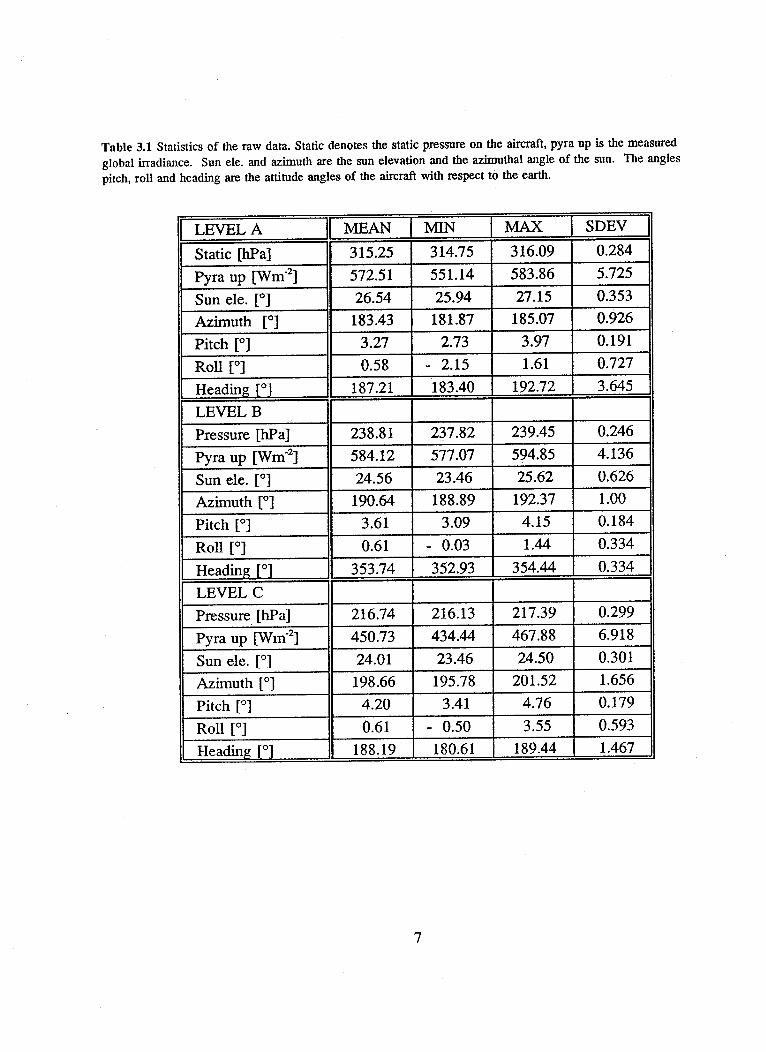
Table 3.1 Statistics of the raw data. Static denotes the static pressure on the aircraft, pyra up is the measured
global irradiance. Sun ele. and azimuth are the sun elevation and the azimuthal angle of the sun. The angles
pitch, roll and heading are the attitude angles of the aircraft with respect to the earth.
LEVEL A iMEAN M IN MAX SDEVStatic [hPa] 315.25 314.75 316.09 0.284
Pyra up [Wm- 2] 572.51 551.14 583.86 5.725
Sun ele. [0] 26.54 25.94 27.15 0.353
Azimuth [0] 183.43 181.87 185.07 0.926
Pitch [0] 3.27 2.73 3.97 0.191
Roll [] 0.58 - 2.15 1.61 0.727
Heading [0] 187.21 183.40 192.72 3.645
LEVEL B
Pressure [hPa] 238.81 237.82 239.45 0.246
Pyra up [Wm 2] 584.12 577.07 594.85 4.136
Sun ele. [0] 24.56 23.46 25.62 0.626
Azimuth [0] 190.64 188.89 192.37 1.00
Pitch [0] 3.61 3.09 4.15 0.184
Roll [] 0.61 - 0.03 1.44 0.334
Heading [°] 353.74 352.93 354.44 0.334
LEVEL C
Pressure [hPa] 216.74 216.13 217.39 0.299
Pyra up [Wmn2] 450.73 434.44 467.88 6.918
Sun ele. [°] 24.01 23.46 24.50 0.301
Azimuth [0] 198.66 195.78 201.52 1.656
Pitch [0] 4.20 3.41 4.76 0.179
Roll [°] 0.61 - 0.50 3.55 0.593
Heading [] 188.19 180.61 189.44 1.467
7

4 CALIBRATION PROCEDURE
4.1 Astronomical Parameters
The solar position is a basic input quantity for the equations determining the effect of the
cosine response of a pyranometer and for the correction of the pyranometer data to the horizontal.
Generally, the sun position is not measured directly, but calculated from the time and place where
the observations were carried out. During the airborne observations the geographic longitude and
geographic latitude are obtained from the aircraft's Inertial Navigation System (INS). From these
data plus information about the solar declination and the equation of time, the sun elevation and
azimuth are determined. The well-known equation for the true solar elevation 0 (without
accounting for refraction) and the sun's azimuth a are given below.
0 = arcsin(sin4 sin 5 + cos4 cos coscK) (4.1)
K = (t- 12) + g + X (4.2)
. a sin(s) * sin0 - sin)a = arcsm Cos ---Cos- (4 .3)
cost cos0
The azimuth a is positive from south to west and negative to the east.
The angle 4 is the geographic latitude of the observer, 6 the declination of the sun, and K the
local hour angle of the sun. In Equation 4.2, t is the local time, and X is the difference between
the local longitude and the reference meridian of the time zone. The equation of time is given
8

by g. Both the declination § and the equation of time are functions depending on the day of the
year and are found in the astronomical almanac. For the present investigation the functions are
approximated by Fourier series (Equation 4.4) with five coefficients (Bannehr, 1985) as listed in
Table 4.1.
The extraterrestrial flux intensity Io depends on the sun-earth distance RV (given in relative
distance) and varies throughout the year. The daily value of the flux density is obtained by
applying the squared inverse of RV to Io, which for the mean sun-earth distance is assigned the
value of 1367 Wm 2. The radius vector is also approximated by the periodic function of Equation
4.4.
() A ( 2nnt 3. 2 tnt--- + a n cos + b n
+ Sm'2 : 365 36
Table 4.1 Coefficients for the declination, equation of time and radius vector.
Coef. Declination Eqn. of time Radius vector
ao 0.79020 0.01238 1.00017
a, -22.92297 0.37852 -0.01663
a2 - 0.38859 -3.58074 -1.1968 E-4
a3 - 0.15527 -0.08528 1.5769 E-5
a4 - 0.00987 -0.13513 -1.6053 E-5
as - 0.00390 0.00992 1.2649 E-5
bl 3.92260 -7.36616 -1.1282 E-3
b2 0.04504 -9.22933 1.5840 E-6
b3 0.08285 -0.25052 1.7095 E-5
b4 0.00511 -0.12434 2.0198 E-5
b 0.00373 0.01718 2.3071 E-5.L -
(4.4)
9
The earth's atmosphere refracts the sunlight so that the sun appears slightly higher than it would
without an atmosphere. Therefore, when the radiation data are corrected, the refraction has to
be considered. The refraction term has to be added to the true solar elevation.
Refr(0) = (4.5)exp (h / 27000) tan (45)
Refr(0) denotes the refraction for a certain solar altitude, given in minutes of arc. The aircraft's
flight altitude is h in feet above sea level.
Equation 4.5 for the determination of the refraction (Nautical Almanac, 1981) is suitable for
aircraft observations. It is accurate to within ±0.2' for solar altitudes >10°. Since the refraction
increases with decreasing solar altitude, the error caused by disregarding the correction increases
accordingly. Modeling has been carried out to investigate this error, assuming clear sky
conditions. For a sun elevation of 20° the deviation found was less than 2.5 Wm' 2. A
comparable error could occur as a consequence of drift in the inertial navigation system on the
aircraft, since a position error on the order of minutes of arc is possible.
4.2 Relative and Diffuse Calibration Coefficient
The calibration of the broadband pyranometers is identical to the calibration procedure
performed by Bannehr (1990) for spectral radiation measurements.
As mentioned in the Preface, the pyranometer response is represented by a single calibration
coefficient, which assumes a perfect instrument response with no variations with the solar zenith
angle. Only in this case can the an the calibration factor be specified by one coefficient K' (millivolts
per Watt per square meter). The deviation of the radiometer response from an ideal cosine
10

response is generally caused by non-ideal sensor surface properties and/or optical effects of the
glass hemispheres, which produce different calibration factors for different solar elevations. This
deviation from Lambert's cosine law will be referred to further on as the relative calibration. The
relative calibration is dependent upon the difference between the measured global and diffuse
signal of a pyranometer compared with the direct signal of a reference device (for example, a
pyrheliometer for broad band studies). Multiplying the relative calibration by the direct
calibration factor of the reference instrument for a particular zenith angle converts the
pyranometer signal into the same scale as the reference device. The relative calibration is given
by:
K'(0) = G-D (4.6)sinO I
G = global signal of the instrument to be calibratedD = diffuse signal of the instrument to be calibratedI = direct signal of the reference instrument0 = observed solar altitude (true solar altitude plus refraction)
Strictly speaking, K'(0) applies only to the direct beam signal. For the diffuse signal, a diffuse
calibration coefficient must be derived from the radiance distribution and the cosine response.
The upward facing pyranometer used on the Sabreliner aircraft was calibrated under clear sky
conditions on 3 July 1991. The World Meteorological Organization (Frohlich and London, 1986)
recommends that the calibration of pyranometers should be repeated at least once a year or even
more frequently if unusual performance of the instrument is detected. The pyranometer was set
up, leveled, and the signal was recorded in two-minute averages. At the same time, direct and
diffuse irradiance measurements were collected by a pyrheliometer and a pyranometer equipped
with a shading band. The relative calibration factor K'(0) for sun elevations between 9° and 72°
was then determined according to Equation 4.6 and illustrated by Figure 4.1.
11

1.03
L- 1.02o
.L-s0
LL- I Nl
c0
.1.
0
.- 1.0000
0 0.99. 0
: 0.98
0 10 20 30 40 50 60 70 80 90
Sun Elevation [ ]
Figure 4.1 Relative calibration factor of the upward facing pyranometer.
The pyranometer shows small deviations from an ideal cosine response. For the present case
the deviation of the cosine response of the pyranometer from ideal is less than ±1% and better
than the specification provided by the manufacturer, Eppley Laboratories. The absolute
pyranometer calibration coefficient derived by Eppley Laboratories on 31 October 1988 was 8.00
E-6 V/Wm' 2, which deviates from the calibration coefficient retrieved on 3 July 1991 by 1.7%.
This small change in the calibration coefficient over a time period of almost 3 years can be
expected. Assuming that only the mean value of the calibration coefficient has changed between
the two calibrations, while the cosine response curve has remained constant, for a more precise
data evaluation the calibration factor K'(9) has been approximated by a bicubic spline function
(Press et al., 1989). It should be pointed out that the good cosine response of the instrument
used in this example is not necessarily representative for other instruments and therefore must
be investigated for each instrument. The error caused by using only a single calibration
coefficient instead of incorporating the full cosine response of the pyranometer results in about
±5.5 Wm' 2 for the current investigation.
12
No. 12127. ... I . . . I , , I , . a. _,!.. ! . I I I I t
I I I I I -if 11 5 I I . . I I I . I I I I . . I I I I I I I I I I I I I I I F I I I I
-i
I

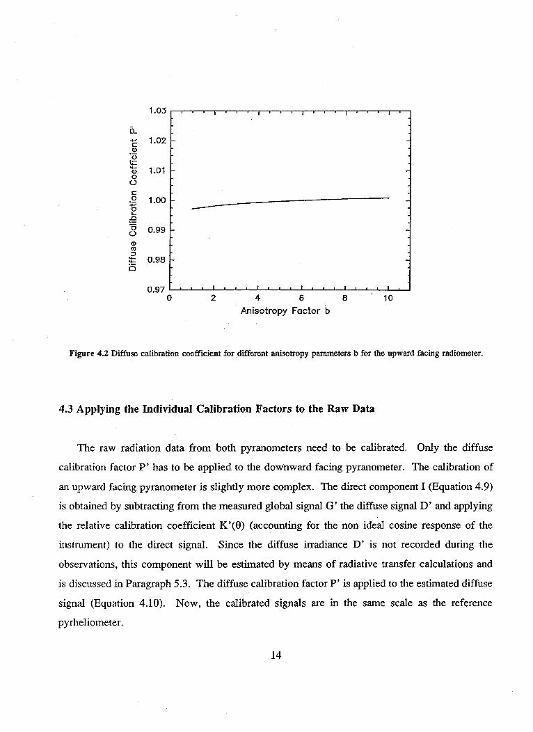
The diffuse component of the measured global signal must be treated differently from the direct
signal. Assuming there are no azimuthal dependencies, the relative diffuse calibration factor P'
can be written as
2
fK'(O) L(O) sin20 dOP / 0 (47)
L( ( + b..1 si
where b is a non-dimensional anisotropy parameter.
For an isotropic sky radiance distribution, the value of b is equal zero. A value of 10
corresponds to a strongly anisotropic radiance distribution. An illustration of the change in the
diffuse calibration factor with increasing anisotropy parameter b for the upward facing radiometer
is given in Figure 4.2. For the evaluation of flight SMT11 an anisotropy parameter b = 3 was
assumed.
13
1.03
a--- 1.020
._-
a 1.0100c
4-0
.Q
o 0.99
(0
0.98
0 Q7
0 2 4 6 8 10
Anisotropy Factor b
Figure 4.2 Diffuse calibration coefficient for different anisotropy parameters b for the upward facing radiometer.
4.3 Applying the Individual Calibration Factors to the Raw Data
The raw radiation data from both pyranometers need to be calibrated. Only the diffuse
calibration factor P' has to be applied to the downward facing pyranometer. The calibration of
an upward facing pyranometer is slightly more complex. The direct component I (Equation 4.9)
is obtained by subtracting from the measured global signal G' the diffuse signal D' and applying
the relative calibration coefficient K'(0) (accounting for the non ideal cosine response of the
instrument) to the direct signal. Since the diffuse irradiance D' is not recorded during the
observations, this component will be estimated by means of radiative transfer calculations and
is discussed in Paragraph 5.3. The diffuse calibration factor P' is applied to the estimated diffuse
signal (Equation 4.10). Now, the calibrated signals are in the same scale as the reference
pyrheliometer.
14
I I I t -- - I -- I I * I 2 I. I . 1 I I I I
. .l l I i

G I - D/sin0
D = D P'
G = IsinE + D
(4.9)
(4.10)
(4.11)
Upon adding the direct and diffuse signals to obtain the global signal, the preprocessing is
complete.
15

5 CORRECTIONS
5.1 Correction for Aircraft Maneuvers
The downward facing radiometer, used to measure the reflected radiation, requires no special
correction scheme because the received signal is only diffuse. Again, more complex is the data
treatment of the upward facing pyranometer. Deviations from straight and level flight make it
necessary to correct the direct radiation data of the upward facing pyranometer for excursions
from the horizontal. The aircraft inertial navigation system provides all the required parameters,
and a geometrical correction for the inclination of the pyranometer can be computed for every
data point. The correction factor which has to be applied to the data is given as follows:
sinO,F = sin- (5.1)
cosO, sin sin( -h) - cos sinp cos( - h)+ sinO cos [cosa
F = correction factor (the direct signal must be multiplied by this quantity)- = solar altitudec = roll angle of the aircraft (positive for left wing up)P = pitch angle (positive for nose up)h = aircraft heading
= azimuthal angle of the sun
Equation 5.1 contains the implicit assumption that the incoming radiation signal is direct
only. If not, this equation is no longer valid, and it would incorrectly determine the direct signal
and thus the global signal.
An example of the correction scheme is given for flight SMT11, level C, in Figure 5.1.
For this example it was assumed that the measured solar irradiance was only direct. The upper
time series shows the computed correction factor determined from Equation 5.1. The second
16

Fliaht SMT11 Level C -1/19/89-
0 100 200 300 400 500 600 700 800 900 1000 111
_A._
0 100 200 300 400 500 600 700 800 900 1000 1101S&mp Ies
Figure 5.1 Illustration of the correction scheme for flight level C.
00 1200 1300
0 1200 1300
17
1 .20
1.18
1.16
o 1.14d
L
<) 1.12
1.10
1 .08
1.06
480
N 470
a 460u
d
- 450LL
440.0
430
N 530
:520
510i- 510
L
- 500
-
O 490
480
_ __ ,--~~~~~~~~~I .M.- -1 I . -- .- - .I I - I
A A-
time series shows the global uncorrected but calibrated data. In the third time series, the
correction factor is applied to the data of the global irradiance time series above. Figure 5.1
explicitly shows how the global irradiance data are smoothed by applying the derived correction
factor to the raw data. Furthermore, the data are not only smoothed but the mean is shifted up
by 60.3 Wm-2 in the present case. The standard deviation was derived after the trend has been
removed by low pass filtering. It was reduced from 4.164 to 0.924 after the correction factor was
applied to the time series. The difference between maximum and minimumn after low pass
filtering decreased at the same time from 27.3 to 7.1 Wmn2. Using the corrected time series as
a reference, the error caused by ignoring the correction for any aircraft maneuvers was as high
as 11.8%.
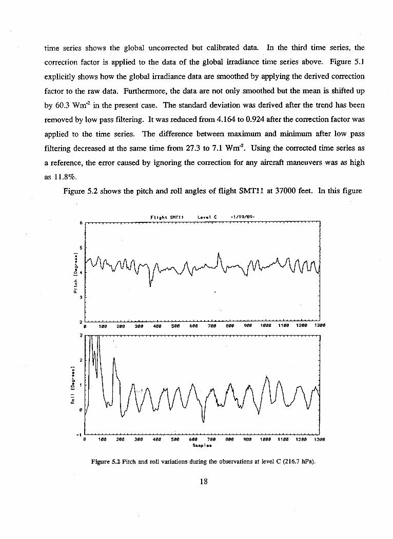
Figure 5.2 shows the pitch and roll angles of flight SMT11 at 37000 feet. In this figure
6
5
L
4
f.Q1
3
2
2
L
t1
01
0
-1
Flight SMT11 Level C -1/19/89-. .. .. . ... . . . .. .. .I . . . . . . .... . , . . ..
I. . .
" I.. . . . . . .. .. .
0 100 200 300 400 500 600 700 800 900 1000 1100 1200 1300Samplem
Figure 5.2 Pitch and roll variations during the observations at level C (216.7 hPa).
18
0 100 200 300 400 500 600 700 600 900 1000 1100 1200 1300.. . . . I . .. . . . . . . . . . . . . . . . . . . . . . . . . . . . . . . . . . . . . . . . . . . . .
I-

the average roll angle is not zero as it should be for a correct INS installation. The results given
in this section demonstrate that an INS misalignment does not influence the effectiveness of the
correction scheme. Similar figures are produced for the traverses A and B. They are found in
Appendix A.
5.2 Installation of the Radiometers
The upward facing instrument is installed on top of the fuselage where the obstructions by
the aircraft are minimized. However, depending on the heading of the aircraft and the solar
position, the radiometer signal can be slightly affected by the aircraft's tail. This should be kept
in mind for the data evaluation.
The installation of the downward facing radiometer is not complicated. Apart from adjusting
it to the mean pitch angle of the aircraft during the observation no special considerations are
required.
Simulations have shown the importance of aligning the upward facing radiometer as close
as possible to the inertial navigation system of the aircraft, because the pitch angle, roll angle,
and aircraft heading provide the input parameters for the correction (Equation 5.1). Even small
deviations cause significant uncertainties when the radiometer data are corrected for the
radiometer inclination during the flight. The order of the error depends on the atmospheric
loading and more strongly on the solar altitude. The error increases for low solar altitudes.
Radiative transfer calculations were performed to investigate this potential error source.
Assuming a total aerosol optical depth T=0.1, an atmospheric water vapor content ppw=l1.5 cm,
an ozone mass 03=0.3 cm, and a surface albedo w=0.12, Table 5.1 shows the percentage error
for different solar altitudes and pyranometer misalignment of ±2°.
19

Table 5.1 Percentage error in global irradiance caused by a misalignment of the pyranometer.
Nominal Solar Tilted(±2° )
Altitude (°) Error (%)
10 ±26.5
30 t 7.2
50 3.3
70 t 1.4
90_24.57 9.3
Figure 5.3 shows the shift of the corrected radiometer data if the instrument is aligned
accurately within ±2°. For the given example, flight SMT1 1, the mean solar altitude was 24.57°.
At this solar altitude a misalignment of ±2° can produce an uncertainty of about 9.3%. Provided
that the solar altitude is 65° for the same misalignment, the error in the global irradiance is of
the order of 2%.
20

600
C<i
4
- 550
Lo s
40
500
4500 50 100 150 200 250 300 350 400 450 500 550 600 650 700 750 800 850
Samples
Figure 5.3 Comparison of misalignments of the upward facing pyranometer (traverse B).
Since there is currently no technique available to retrieve the unknown misalignment in pitch
and roll angles, a numerical iterative procedure was developed to account for any possible
misalignment when the pyranometer is installed on the aircraft. The idea is based on the fact that
the global irradiance received by the sensor of the radiometer under clear skies and at a fixed
altitude is almost independent of the direction in which the aircraft flies. Only trends due to
changing solar altitude are expected. For the case where the instrument is not properly aligned,
systematic changes in the global irradiance signal will occur when the aircraft flies in different
directions. Fortunately, a flight pattern was available where the heading changed from 302° to
333° and then to 69°, so that data at one altitude and three different directions are accessible to
derive the pitch and roll misalignment errors, Ap and Ar. The method uses Equation 5.1 as a
basis, which corrects the radiometer data by the factor F for the deviation from a straight flight
during the observations. The correction factor F is derived from the observed quantities (sun
elevation, azimuth, pitch and roll angles of the aircraft) and assumed values for delta pitch, Ap,
21
A. ! n6D50

and delta roll angles, Ar for the whole traverse and is applied to the radiometer data. The
corrected time series is low-pass filtered to remove any trends due to changing solar altitude.
The data are stored temporarily. Then the low pass filtered time series is subtracted from the
unfiltered time series to obtain a series of higher frequency residuals. The standard deviation is
determined and stored together with the assumed delta pitch and delta roll angles. This procedure
is repeated between two defined Ap and Ar bounds, namely ±3°. The actual delta pitch and delta
roll angles are found by searching for the smallest standard deviation of the corrected time series.
The delta pitch and delta roll angles retrieved by the numerical procedure were Ap=-0.48° and
Ar=-0.08°. By adding these values to the recorded pitch and roll angles, the pyranometer is
aligned with respect to the aircraft inertial system. The numerical procedure was also tested
using only two flight legs and the results were unsatisfactory. It was found that satisfactory
results are achievable only if all three flight traverses are utilized in the delta pitch and delta roll
determination.
5.3 Incorporating the Diffuse Irradiance into the Correction Procedure
Currently, there is no instrumentation or shading device installed on the aircraft that allows
the measurement of diffuse irradiance. Therefore it is not possible to separate the direct
irradiance from the global irradiance which is stringently necessary to correct properly for aircraft
attitude changes. For the case that the observations have been carried out under conditions of
clear skies, a vertical profile of the ratio of diffuse irradiance to global irradiance can be
estimated from a radiation model, and thus the diffuse irradiance can be estimated. For the
present investigation such simulations for different atmospheric conditions have been undertaken.
The model used is Forgan's (1989) simple multi-layer spectral radiation model for clear skies.
It provides the upwelling and downwelling radiation fluxes for n defined pressure levels. The
simulations are performed for two different cases, each with 9 layers between surface pressure
and 100 hPa and five different solar altitudes between 10° and 90°. The first case used a high
total aerosol optical depth of 0.25 and a high total atmospheric precipitable water of 3.0 cm. The
second case used a low total aerosol optical depth of 0.10 and a low total ppw value of 0.5 cm.
22
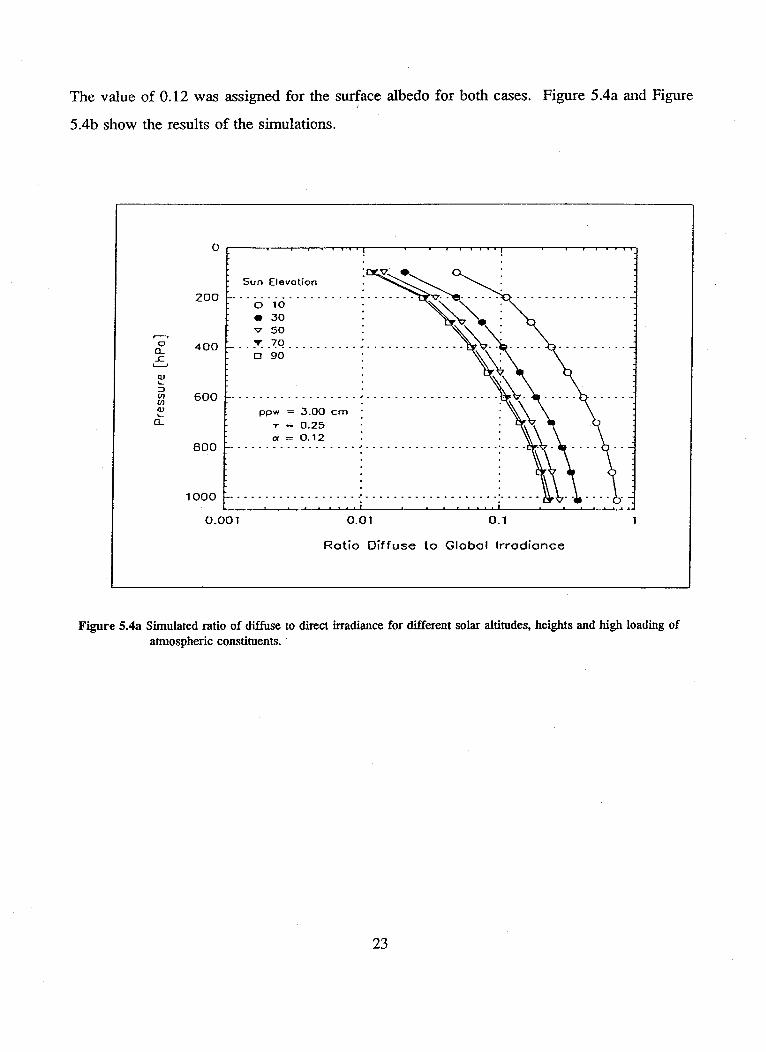
The value of 0.12 was assigned for the surface albedo for both cases. Figure 5.4a and Figure
5.4b show the results of the simulations.
Figure 5.4a Simulated ratio of diffuse to direct irradiance for different solar altitudes, heights and high loading ofatmospheric constituents.
23

0
Figure 5.4b Simulated ratio of diffuse to direct irradiance for different solar altitudes, heights and low loading of
atmospheric constituents.
These two graphs show the variability of the ratio of diffuse to global irradiance D/G(O) for
high and low aerosol loading and water vapor for different sun elevations and pressure levels
under clear sky conditions. These data are used now to obtain an estimate of the diffuse
irradiance D' for each flight level.
D' = G. () * D (5.2)G(0)
In Equation 5.2, the estimated diffuse irradiance is D'. Gm(O) denotes the measured global
24
Sun Elevation
0 10*30v 50
... . . .7.Q...........0 90
ppw = 0.50 cmT = 0-10a = 0.12
200
ci,L 600
o_
CL
c-
800
1000
0.001 0.01 0.1 1
Rotio Diffuse to Globol Irrodionce
I - . . I .7 I I . I I I I . r---r -I- r-
i
III
I- - - -
I . -. . . . I . . . . I - - A. . . I. . . . . . . . . . ..
irradiance. The ratio of diffuse to global irradiance is given by D/G(0). By subtracting from the
measured global irradiance G. the estimated diffuse irradiance, the direct irradiance I for the
actual solar altitude is obtained. The correction factor F (Equation 5.1) is now applied to the
direct signal and the diffuse irradiance is added to the corrected time series. Since the flight
levels A, B and C of SMT1 1 were in the lower stratosphere, the diffuse irradiance for clear sky
conditions is small and was estimated from the multi-layer radiation model as 7.5% (for level A)
of the total irradiance at the solar altitude of 26.5°. No significant differences are found by
incorporating the diffuse irradiance into the correction. However, it must be emphasized that
for most occasions the assumption of completely clear skies is not appropriate. Even thin cirrus
clouds in the area of the observations cause a strong increase in the forward scattering direction
or diffuse irradiance. This can lead to higher or lower global irradiance than is found under clear
sky conditions.
Under clear skies, the global irradiance increases with height due to decreasing extinction of
the solar radiation. In the present investigation, the mean corrected values for the global
irradiance derived are for level A 620.3 Wm`2, for level B 537.9 Wm' 2 and for level C (highest
flight leg) 511.0 Wm'2. Obviously, the expected increase of the global irradiance with increasing
height does not occur and shows a reversed behavior. This feature might be caused by changing
solar altitude with time, not including the real diffuse irradiance but using only an estimate in
the correction procedure, changing location for the observations, or a combination of all three.
Since the diffuse irradiance was not measured during mission SMTI 1, no statement about this
parameter can be made, and therefore no information about clouds is available from
measurements on the aircraft. The observed global irradiance is treated as a direct signal only.
Changes of the global irradiance due to the different locations at the altitudes flown are regarded
as small and will not be discussed further. The change of the solar elevation has a strong effect
on the global irradiance, even if the observations are carried out over a short period of time.
This effect is only small around noon. Therefore, to derive the solar heating rate or the
absorption of a layer, the radiation data must be normalized to a mean solar altitude before the
radiation fluxes can be computed. The required normalization will be discussed in the following
paragraph.
25
5.4 Normalization to the Mean Air Mass
After the calibration is performed and the attitude variations of the aircraft have been taken
into account, the data are referenced to a standard air mass of the flight before the flux
divergence can be calculated. The standard air mass for the correction will be referred to as the
middle air mass of the flight. Four assumptions are made:
1) The total optical depth T, is constant during the observations,
2) the ratio of direct to diffuse irradiance I/D is constant for each level
and independent of the sun elevation 0, and hence
3) the albedo ac is constant during the flight.
4) A further assumption required is that the water vapor absorption can be
described by the law of Lambert-Bouguer-Beer
I' = Iie t -ine osine (5.3)
trot = -ln(4) sinOt (5.4)
D=(ll -i /(5.5)
G' = I; sin + D (5.6)
U. = a, Gil (5.7)
26

0i is the mean solar altitude of the flight level and Q0 is the middle solar altitude of the flight as
a whole. ty is the total optical depth, 1 is the extraterrestrial flux density, and Ii, Di, and Gi are
the direct, diffuse and global radiation. By calculating Di', G1' and U,' for each level, the data
are converted into the same referenced solar altitude O. U1' denotes the reflected radiation.
Using the mean corrected global irradiance data and normalizing them to the mean solar
altitude of 24.57° (mean solar elevation of the analyzed data set) yields for level A 576.3 Wm'2
(lowest cruising level), for level B 537.9 Wm'2 and for level C 522.3 Wm' 2. Despite having all
corrections applied, the radiation data still do not increase with height for the three flight levels
as can be expected from the model (clear sky conditions). This result can be caused by the
limited accuracy achievable with the pyranometer and/or the presence of clouds in the area of
observation, enhancing the diffuse and global irradiance. An agreement better than 1.5% is
achieved between the observed global irradiances and model results for level B. For level C the
observed values are 3.0% smaller than the modeled fluxes. For level A the measured global
irradiance deviates by 10.3%. This large difference in the global irradiances can be explained
by the presence of cirrus clouds in the region of observation, which were indicated in the satellite
picture on this day. From the data analysis and modeling results, the clouds appear to be below
flight level B. The assumption of a clear sky is therefore applicable, so the modeled ratio of
diffuse to global irradiance cannot be used to derive the diffuse irradiance and it is not
incorporated in the correction procedure illustrated here. If the true diffuse irradiance is not
known, the applied correction (Equation 5.1) leads to false results. This example illustrates the
importance of measuring the diffuse irradiance explicitly and not deriving it implicitly by
radiative transfer calculations that presume certain atmospheric conditions.
27
6 Conclusions and Reconunendations
The procedure described for the calibration and correction of pyranometer data in this
technical note is aimed at improving of the current basic data treatment. The observed error in
the pyranometer cosine response was less than 1% for solar altitudes between 9° to 72°. Ignoring
cosine corrections the data results in an error of about ±5.5 Wm- 2 for the current investigation.
The calibration should be repeated at least once a year to detect and compensate for drifts of the
instruments.
The correction technique for the upward facing pyranometer that accounts for aircraft
maneuvers improved the accuracy of the radiometer data drastically. The absolute deviation was
reduced by 11.7 Wm"2 on average for all three levels and showed the smoothing effect of the
correction. More significant, however, was the shift of the mean global irradiance values. For
level C the shift was as high as 60.3 Wmn2. When applying the correction factor to the radiation
data, it must be realized that such a correction cannot be performed for large inclinations of the
aircraft. For large pitch or roll angles the pyranometer receives in addition to the downwelling
radiation also upwelling radiation, for which it is not possible to correct. It is suggested that data
should be used only if the pitch and roll angles of the aircraft are within ±6°.
If the upward facing pyranometer is misaligned by ±2° compared to the aircraft inertial
navigation system, the error in the global irradiance can be up to ±11% for a solar altitude of 20°
according to radiative transfer calculations. Therefore, care should be taken to eliminate this
uncertainty. The numerical procedure described can be used to derive the pitch and roll angle
misalignment errors and therefore to account for this source of uncertainty. The downward
facing pyranometer should be adjusted to the mean pitch angle of the aircraft in order to
minimize the detection of the downwelling radiation.
The main recommendation concluded from the data analysis is that the diffuse irradiance
should be measured in addition to the observed global irradiance in order to make a more
28

efficient use of the correction procedure. Diffuse irradiance could be obtained by designing a
rotating or flipping shading device. Including the diffuse irradiance in the group of radiometric
quantities has some further benefits. Namely, by measuring the global and diffuse irradiance,
the direct irradiance, and therefore the total optical depth can be determined, which is an
important input parameter for climatological models.
A matter not discussed in this technical note should be mentioned, as some future work is
still necessary. The pyranometer output is known to be sensitive to differential heating between
the dome of the instrument and the cold junction of the thermopile. This effect for pyrgeometers
has been discussed by many scientists. According to Albrecht and Cox (1977), the error of the
long wavelength radiation can be reduced by 60 Wm'2. For this technique, the dome and the sink
temperatures of the pyrgeometer are measured in addition to the radiometer output. Since the
pyranometer and pyrgeometer are identical instruments apart from the spectral filtering
mechanism, a similar correction procedure can be derived for the pyranometers if the dome and
sink temperatures of the pyranometer are measured.
29
REFERENCES
Albrecht, B. and Cox, S.K.: 1976, Procedure for Improving Pyrgeometer Performance,J. Appl. Meteor., 16, 188-197
Bannehr, L.: 1985, Die Extinktion der direkten Solarstrahlung im aktinometrischenSpektralbereich, Diplomarbeit, Freie Universitat Berlin, 85 pp.
Bannehr, L.: 1990, Airborne Spectral Radiation Measurements in South Australia, Ph.D. Thesis,Flinders University of South Australia, 180 pp.
Eppley Laboratory Inc.: (no date), Instrumentation for the Measurement of the Components ofSolar and Terrestrial Radiation, Newport, R.I. 02840, USA, 12 pp.
Forgan, B.W.: 1979, The Measurement of Solar Irradiance: Instrumentation and Measurementin the Adelaide Region, Ph.D. Thesis, Flinders University of South Australia, 380 pp., 1979
Forgan, B.W.: 1989, Personal Communication
Frollich, C. and London, J. (ed.): 1986, Revised Instruction Manual on Radiation Instrumentsand Measurements, WCRP Publications Series No. 7, WMO/TID-No. 149
Press, W.H., Flannery, B.P., Teukolsky, S.A. and Vetterling, W.I.: 1989, Numerical Recipes,Cambridge University Press, 702 pp.
30
APPENDIX A
Illustration of the correction scheme for the flight levels A and B
31
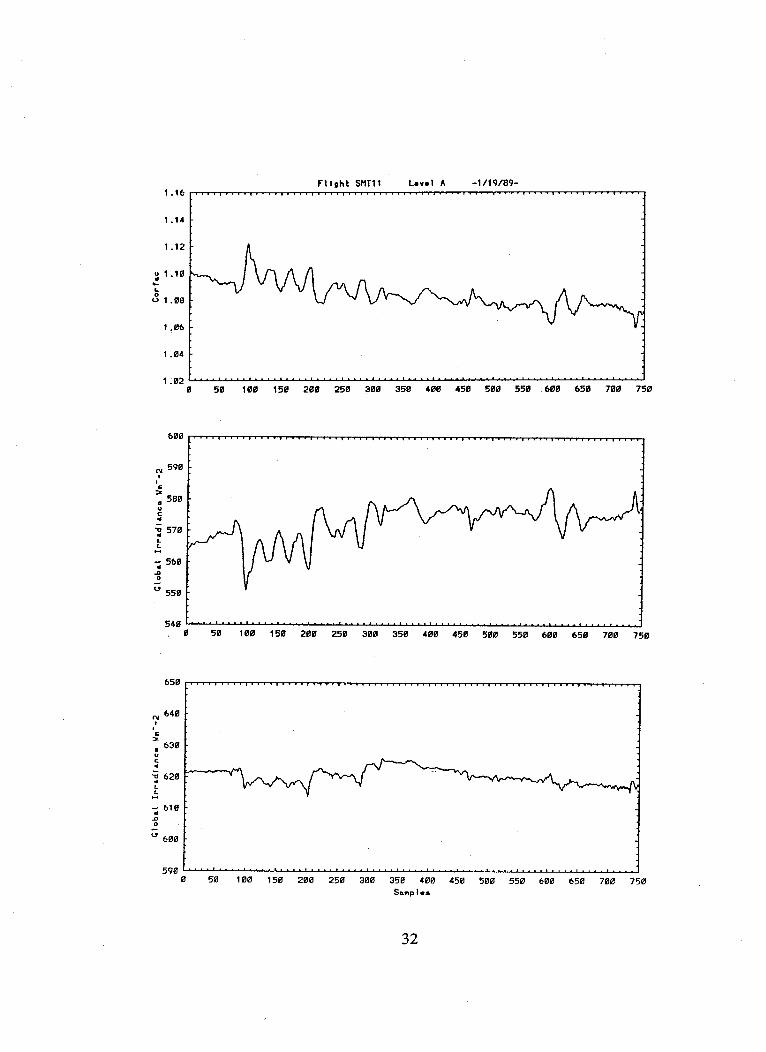
Flight SMiT11 Lovel A -1/19/89-
0 50 100 150 20 2 250 300 350 400 450 500 550 600 650 700 750Samp les
32
1 .16
1 .14
1.12
o 1 .10
L
uJ 1.08
1 .06
1 .04
1 .02
, 590
a 580u
a 570LL
- 560
0
550
540i
650
c 640
f-
630
4
- 620
LI.
- 610
0-05 600
590
.-- .-- --- --- --- --- -- - --- - -- --
& Md,2
I

Flight SMT11 Level A -1/19/89-
50
0 50 100 150 200 250 300 350 400 450 500 550 600 650 700 750
Samples
33
5
Io
A4
UC
3
20 50 100 150 200 250 300 350 400 450 500 550 600 650 700 7
U
3-1
-2-21
. . . . . . . . . . . . . . . . . . . . . . . . . . . . . . . . . .. . . . . . . . . . . . . . . . . . . . . . . . . . . . . . . . .
Flight SMT11 L.vel B -1/19/89--- ------- ------. . . . . . . . . . . . . . . . . . . . .. . I . . . . . . . . . . . . . . . . . . . . . . . . . . . . . . I., ..
0 50 100 150 200 250 300 350 400 450 500 550 600 650 700 750 800 850
0 50 100 '150 200 250 300 350 400 450 500 550 600 650 700 750 800 850
0 50 100 150 200 250 300 350 400 450 500 550 600 650 700 750 800 850Sump es
34
1 .00
.98
.96
.94
.92
.90
.88
.86
L0u
0119
600
590Cc
- 580L
L
- 570
-0
K60
550
560
3
550
C
' 540d
L-.4
- 530
-o
520
r10 I
. . . . . . . . . . . . . . . -. . . . . . . . . . . . L . .- . ..- .. .. . . . . . .
. . . . . . . . . . . . . . . . . . . . . . . . .. . . . . . I I , I I I . I I I I . I I I I . . . . . .. . .. . .. . . . . . . . . . . .. . .. . . I . . . .
.. ... .... ... . . . ... .. .. .. .. . ... ... .... ... . . . .. . . .. . .. . . . . . .... .
,- - - - - -- - - - - . . . . . . . . . . . . . . . . . . . . . . | . . .... . . . . . . . . . . . . . . . . . . . . . . . . . . . . . . . . . . . . . . . s. . O r. . . .r.
. .. . . . . .. I I . . . . . . . . .. . . ... I -. . . . . 1 I · 1 ·· ii t -. i · Il · · I . _. .- · I I I· 1 L I-. ..
I
dL 4 a"1
;; i; Lo -
e
E-M
;IV Ii
--------- - -- -- --- --- --- --
Flight SMTI! Level 8 -1/19/89-0
Samples
35
0
5
a
o
-c4L
0I
04
E.
3
2
3
2
U
g1
0I.
0
-1
500 50 100 150 200 250 300 350 400 450 500 550 600 650 700 750 600 8
. . . . . . . . . . . .. . . . . . . . . . . . . . . . . . . . . . .7 777 7I I ~r7 77 7 7I T 17
Pi/"J