Prepared by: Jamal Husein C H A P T E R 5 © 2005 Prentice Hall Business PublishingSurvey of...

© 2005 Prentice Hall Business Publishing© 2005 Prentice Hall Business Publishing Survey of Economics, 2/eSurvey of Economics, 2/e O’Sullivan & SheffrinO’Sullivan & Sheffrin

Prepared by: Jamal Husein

C H A P T E R

55Perfect Competition: Short Run and Long Run

© 2005 Prentice Hall Business Publishing Survey of Economics, 2/e O’Sullivan & Sheffrin 2

Perfectly Competitive MarketPerfectly Competitive MarketPerfectly Competitive MarketPerfectly Competitive Market

1. There are many firms.

2. The product is standardized, or homogeneous.

3. Firms can freely enter or leave the market in the long run.

4. Each firm takes the market price as given.

A perfectly Competitive market ischaracterized by:


The Short-run Output DecisionThe Short-run Output DecisionThe Short-run Output DecisionThe Short-run Output Decision

The firm’s objective is to produce the level of output that will maximize profit.

Economic profit = total revenue (TR) minus total economic cost (TC).

Total revenue = price × quantity sold. The cost structure of the business firm

is the same as the one we studied earlier.


The Firm’s TC Structure (Revisited)The Firm’s TC Structure (Revisited)The Firm’s TC Structure (Revisited)The Firm’s TC Structure (Revisited)

The shape of the total cost curve comes from diminishing returns in the short run.

ST C T FC ST VC Short-run Total Cost = Total

Fixed Cost +Short-run Total Variable Cost

Total CostShort-run

CostVariable

Total

CostFixed

MinuteRakes perOutput:

STCTVCFCQ

360360

448361

4812362

5115363

5620364

6327365

7236366

8448367

10165368

12690369

1661303610


The Revenue Structure of the The Revenue Structure of the Competitive Business FirmCompetitive Business FirmThe Revenue Structure of the The Revenue Structure of the Competitive Business FirmCompetitive Business Firm

The perfectly competitive firm is a price-taking firm. This means that the firm takes the price from the market.

As long as the market remains in equilibrium, the firm faces only one price—the equilibrium market price.


Computing the Total Revenue of a Computing the Total Revenue of a Price-takerPrice-takerComputing the Total Revenue of a Computing the Total Revenue of a Price-takerPrice-taker

Since the perfectly competitive firm faces a constant price, the shape of its total revenue is an upward-sloping line. Total revenue changes only with changes in the quantity sold.

($)Revenue

Total

Price ($)MinuteRakes perOutput:

TRPQ

0.00250

25.00251

50.00252

75.00253

100.00254

125.00255

150.00256

175.00257

200.00258

225.00259

250.002510

0

50

100

150

200

250

Co

st

in $

0 1 2 3 4 5 6 7 8 9 10 Output: Rakes per minute

Total Revenue


The Totals Approach to Profit MaximizationThe Totals Approach to Profit MaximizationThe Totals Approach to Profit MaximizationThe Totals Approach to Profit Maximization

To maximize profit, a producer finds the largest gap between total revenue and total cost. ProfitTotal Cost

Short-run($)

RevenueTotal

MinuteRakes per

Output:

STCTRQ

-36360.000

-194425.001

24850.002

245175.003

4456100.004

6263125.005

7872150.006

9184175.007

99101200.008

99126225.009

84166250.0010


The Marginal ApproachThe Marginal ApproachThe Marginal ApproachThe Marginal Approach

The other way to decide how much output to produce involves the marginal principle.

Marginal PRINCIPLEIncrease the level of an activity if its marginal benefit exceeds its marginal cost, but reduce the level if the marginal cost exceeds the marginal benefit. If possible, pick the level at which the marginal benefit equals the marginal cost.


Marginal RevenueMarginal RevenueMarginal RevenueMarginal Revenue

The benefit of producing and selling rakes is the revenue the firm collects. If the firm sells one more rake, total revenue increases by $25.

Marginal benefit = marginal revenue = market price


A firm maximizes profit in accordance with the marginal principle—by setting marginal revenue (or market price) equal to marginal cost.

ProfitCostMarginalShort-run

Price ($)Revenue =Marginal

MinuteRakes perOutput:

SMCPQ

-36-250

-198251

24252

243253

445254

627255

789256

9112257

9917258

9925259

84402510

The Marginal Rule for Profit MaximizationThe Marginal Rule for Profit MaximizationThe Marginal Rule for Profit MaximizationThe Marginal Rule for Profit Maximization


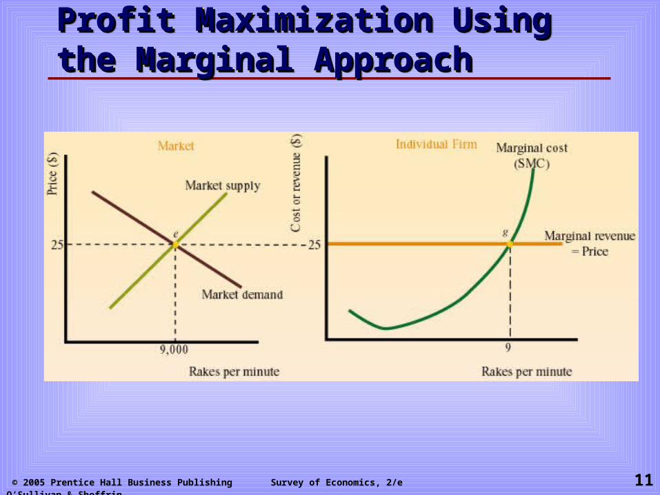
Profit Maximization Using the Profit Maximization Using the Marginal ApproachMarginal ApproachProfit Maximization Using the Profit Maximization Using the Marginal ApproachMarginal Approach


Economic ProfitEconomic ProfitEconomic ProfitEconomic Profit

Profit per unit equals revenue per unit (or price) minus cost per unit (or average total cost).

($25 - $14) = 11

Total economic profit equals:(price – average cost) × quantity produced

($25 - $14) x 9 = $99


Shut-down DecisionShut-down DecisionShut-down DecisionShut-down Decision

The firm should continue to operate if the benefit of operating (total revenue) exceeds the cost of operating, or total variable cost.

TR = (P × Q) must be greater than STVC = SAVC × Q, therefore,

If P > SAVC, the firm should continue to operateIf P < SAVC, the firm should shut down


The Shut-down DecisionThe Shut-down DecisionThe Shut-down DecisionThe Shut-down Decision When price drops to

$9, the firm adjusts output down to 6 rakes per minute to maintain P=SMC.

The firm suffers a loss, but since price is greater than AVC, the firm continues to operate.

The average variable cost of producing 6 rakes per minute is $6.


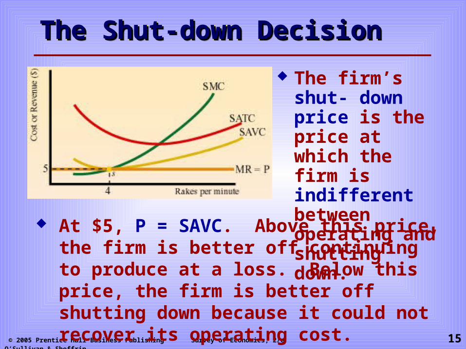
The Shut-down DecisionThe Shut-down DecisionThe Shut-down DecisionThe Shut-down Decision

The firm’s shut- down price is the price at which the firm is indifferent between operating and shutting down.

At $5, P = SAVC. Above this price, the firm is better off continuing to produce at a loss. Below this price, the firm is better off shutting down because it could not recover its operating cost.


Short-run Supply CurveShort-run Supply CurveShort-run Supply CurveShort-run Supply Curve

The firm’s short-run supply curve shows the relationship between the market price and the quantity supplied by the firm over a period of time during which one input—the production facility—cannot be changed.


The Firm’s SR Supply CurveThe Firm’s SR Supply CurveThe Firm’s SR Supply CurveThe Firm’s SR Supply Curve For any price above

the shut-down price, the firm adjusts output along its marginal cost curve as the price level changes.

The short-run supply curve is the firm’s SMC curve rising above the minimum point on the SAVC curve.

Below the shut-down price, quantity supplied equals zero.


The Market Supply CurveThe Market Supply CurveThe Market Supply CurveThe Market Supply Curve

The short-run market supply curve shows the relationship between the market price and the quantity supplied by all firms in the short run.


A Market in Long-run EquilibriumA Market in Long-run EquilibriumA Market in Long-run EquilibriumA Market in Long-run Equilibrium

1. The quantity of the product supplied equals the quantity demanded

2. Each firm in the market maximizes its profit, given the market price

3. Each firm in the market earns zero economic profit, so there is no incentive for other firms to enter the market

A market reaches a long-run equilibrium when three conditions hold:



In short-run equilibrium, quantity supplied equals quantity demanded and each firm in the market maximizes profit.

In addition to the conditions above, in long-run equilibrium the typical firm earns zero economic profit so there is no further incentive for firms to enter the market.



In long-run equilibrium, price = marginal cost (the profit-maximizing rule), and price = short-run average total cost (zero economic profit).


The LR Supply Curve for an The LR Supply Curve for an Increasing-cost IndustryIncreasing-cost IndustryThe LR Supply Curve for an The LR Supply Curve for an Increasing-cost IndustryIncreasing-cost Industry

An increasing-cost industry is an industry in which the average cost of production increases as the total output of the industry increases.

The average cost increases as the industry grows for two reasons:

Increasing input prices Less productive inputs


Industry Output and Average Industry Output and Average Production CostProduction CostIndustry Output and Average Industry Output and Average Production CostProduction Cost

Number of Firms

Industry Output

Rakes per Firm

Typical Cost for Typical Firm

Average Cost per

Rake

50 350 7 $70 $10

100 700 7 84 12

150 1,050 7 96 14

The rake industry is an increasing-cost industry because the average cost of production increases as the total output of the industry increases.


Drawing the Long-run Market Supply Drawing the Long-run Market Supply CurveCurveDrawing the Long-run Market Supply Drawing the Long-run Market Supply CurveCurve

Each point on the long-run supply curve shows the quantity of rakes supplied at a particular price (i.e., at a price of $12, 100 firms produce 700 rakes).

The long-run industry supply curve is positively-sloped for an increasing cost industry.


SR Increase in Demand and the SR Increase in Demand and the Incentive to EnterIncentive to EnterSR Increase in Demand and the SR Increase in Demand and the Incentive to EnterIncentive to Enter

An increase in market demand puts upward pressure on price. As price increases, there is an opportunity to earn profit in the short run, and the industry attracts new firms.


The Long-run Effects of an Increase in The Long-run Effects of an Increase in DemandDemandThe Long-run Effects of an Increase in The Long-run Effects of an Increase in DemandDemand

In the short-run, firms respond to the increase in demand by adjusting output in their existing production facilities, and the price adjusts from $12 to $17.


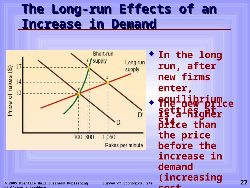
The Long-run Effects of an Increase in The Long-run Effects of an Increase in DemandDemandThe Long-run Effects of an Increase in The Long-run Effects of an Increase in DemandDemand

In the long run, after new firms enter, equilibrium settles at $14.

The new price is a higher price than the price before the increase in demand (increasing cost industry).


Long-run Supply Curve for an Long-run Supply Curve for an Constant-cost IndustryConstant-cost IndustryLong-run Supply Curve for an Long-run Supply Curve for an Constant-cost IndustryConstant-cost Industry

In a constant-cost industry, firms continue to buy inputs at the same prices.

The long-run supply curve is horizontal at the constant average cost of production.

After the industry expands, the industry settles at the same long-run equilibrium price as before.


Long-run Supply Curve for the Ice Long-run Supply Curve for the Ice IndustryIndustryLong-run Supply Curve for the Ice Long-run Supply Curve for the Ice IndustryIndustry

In the long-run, the price of ice returns to its original level.

An increase in the demand for ice increases the price of ice to $5 per bag.

Prepared by: Jamal Husein C H A P T E R 5 © 2005 Prentice Hall Business PublishingSurvey of...

Documents

Transcript of Prepared by: Jamal Husein C H A P T E R 5 © 2005 Prentice Hall Business PublishingSurvey of...