Prepared by Jack Flicker Jay Johnson - Solar America … · Prepared by Jack Flicker Jay Johnson...

Analysis of Fuses for“Blind Spot” Ground

Fault Detection in Photovoltaic

Power Systems

Prepared by

Jack FlickerJay Johnson

Sandia National Laboratories

June 2013

Solar America Board for Codes and Standardswww.solarabcs.org

2 Solar America Board for Codes and Standards Report

DISCLAIMER

This report was prepared as an account of work sponsored by an agency of the United States government. Neither the United States government nor any agency thereof, nor any of their employees, makes any warranty, express or implied, or assumes any legal liability or responsibility for the accuracy, completeness, or usefulness of any information, apparatus, product, or process disclosed, or represents that its use would not infringe privately owned rights. Reference herein to any specific commercial product, process, or service by trade name, trademark, manufacturer, or otherwise does not necessarily constitute or imply its endorsement, recommendation, or favoring by the United States government or any agency thereof. The views and opinions of authors expressed herein do not necessarily state or reflect those of the United States government or any agency thereof.

3

EXECUTIVE SUMMARY

A 2012 Solar America Board for Codes and Standards (Solar ABCs) publication, The Ground-Fault Protection Blind Spot: Safety Concern for Larger PV Systems in the U.S. (Brooks, 2012), revealed that undetected faults on grounded PV array conductors were an initial step in a sequence leading to two well-publicized rooftop fires. In that paper, the theoretical detection limits of traditional ground fault protection systems were discussed but not explored in depth.

To further the analysis of ground fault protection in photovoltaic (PV) systems, scientists from Sandia National Laboratories developed a functional circuit model of the PV system including modules, wiring, switchgear, grounded or ungrounded components, and the inverter. This model was implemented using the Simulation Program with Integrated Circuit Emphasis (SPICE) modeling language. The Sandia Technical Report, Photovoltaic Ground Fault and Blind Spot Electrical Stimulations (Flicker & Johnson, 2013), presents the complete derivation of the Sandia PV System SPICE model and the results of parametric fault current studies with varying array topologies, fuse sizes, and fault impedances.

This Solar ABCs report contains the subsection of the Sandia technical report that focuses on blind spot ground faults to the grounded current-carrying conductor. The behavior of the array during these faults is studied for a range of ground fault fuse sizes to determine if reducing the size of the fuse improves ground fault detection sensitivity. Results of simulation studies show that reducing the amperage rating of the protective fuse does increase fault current detection sensitivity without increasing the likelihood of nuisance trips. However, this effect reaches a limit as fuses become smaller and their internal resistance increases to the point of becoming a major element in the fault current circuit.

Analysis of Fuses for “Blind Spot” Ground Fault Detection in Photovoltaic Power Systems

http://www.solarabcs.org/blindspot

http://www.solarabcs.org/blindspot

http://energy.sandia.gov/wp/wp-content/gallery/uploads/SAND2013-3459-Photovoltaic-Ground_Fault-andBlind-Spot-Electrical-Simulations.pdf

http://energy.sandia.gov/wp/wp-content/gallery/uploads/SAND2013-3459-Photovoltaic-Ground-Fault-and-Blind-Spot-Electrical-Simulations.pdf


TABLE OF CONTENTS

DISCLAIMER ................................................................................................................ 2

EXECUTIVE SUMMARY ............................................................................................... 3

AUTHOR BIOGRAPHIES ............................................................................................. 5

SOLAR AMERICA BOARD fOR CODES AnD STAnDARDS ....................................... 5

ACKnOWLEDGMEnT .................................................................................................. 5

InTRODUCTIOn .......................................................................................................... 6

AnALYTICAL AnALYSIS Of GROUnD fAULT DETECTIOn LIMITS ........................... 7

Effects of Parasitic Cable and fuse Impedances in PV Arrays .............................. 7

Leakage Currents ..................................................................................................... 8

Detection of Blind Spot fault With GfPDs ........................................................... 10

nUMERICAL SIMULATIOnS Of BLInD SPOT fAULTS ............................................. 15

PV Array Simulation Setup .................................................................................... 15

Simulation Results ................................................................................................. 16

GfPD Current During High-Impedance Blind Spot Ground faults .................... 18

Parametric Study of GfPD Current ....................................................................... 21

SUMMARY AnD COnCLUSIOnS .............................................................................. 26

ACROnYMS ............................................................................................................... 27

REfEREnCES ............................................................................................................. 28

5

AUTHOR BIOGRAPHIES

Jack FlickerSandia National Laboratories

Jack Flicker is a postdoctoral appointee at Sandia National Laboratories. His work at Sandia National Laboratories focuses on photovoltaic system and inverter com-ponent reliability. Prior to joining Sandia National Laboratories in 2011, his Ph.D. research at the Georgia Institute of Technology focused on designing, fabricating, and testing cadmium telluride (CdTe) substrate configuration solar cells paired with vertically aligned carbon nanotubes for back surface light trapping.

Jay JohnsonSandia National Laboratories

Jay Johnson is a senior member of the technical staff at Sandia National Laboratories and has researched renewable energy and energy efficiency technologies for the last eight years. He has experience working on solar thermal and wind energy systems at the National Renewable Energy Laboratory (NREL), smart grid and demand response control algorithms at the Palo Alto Research Center (PARC), fuel cell membrane manufacturing at the Georgia Institute of Technology, and, for the last three years, he has run Sandia National Laboratories’ photovoltaic arc-fault and ground fault detection and mitigation program. Mr. Johnson represents Sandia National Laboratories on the Solar ABCs steering committee and is actively involved in the development of codes and standards for PV systems in the United States and abroad.

Solar America Board for Codes and Standards

The Solar America Board for Codes and Standards (Solar ABCs) provides an effective venue for all solar stakeholders. A collaboration of experts formally gathers and prioritizes input from groups such as policy makers, manufacturers, installers, and large- and small-scale consumers to make balanced recommendations to codes and standards organizations for existing and new solar technologies. The U.S. Department of Energy funds Solar ABCs as part of its commitment to facilitate widespread adoption of safe, reliable, and cost-effective solar technologies.

Solar America Board for Codes and Standards website:

www.solarabcs.org

Acknowledgment

This material is based upon work supported by the U.S. Department of Energy under Award Number DE-FC36-07GO17034. This work was funded by the DOE Office of Energy Efficiency and Renewable Energy. Sandia National Laboratories is a multi-program laboratory managed and operated by Sandia Corporation, a wholly owned subsidiary of Lockheed Martin Corporation, for the U.S. Department of Energy’s National Nuclear Security Administration under contract DE-AC04-94AL85000.



Introduction

A PV array ground fault is an electrical short circuit between one or more of the array’s conductors and earth ground. Such faults are usually the result of mechanical, electrical, or chemical degradation of photovoltaic (PV) components or mistakes made during installation. In order to protect the array against continued operation during a ground fault event, a ground fault protection device (GFPD) or ground fault detector/interrupter (GFDI) is used to detect ground fault currents (Wiles, 2012).

Recently, a detection limit, or “blind spot,” in traditional ground fault protection systems has been identified for the direct current- (DC-) grounded, alternating current- (AC-) isolated PV systems, most common in the United States (Wiles, 2012). This blind spot occurs when the grounded current-carrying conductor (CCC) is faulted to the equipment grounding conductor (EGC) as shown in Figure 1.

Figure 1. Schematic for an array with parasitic impedances measured from a fielded system and non-zero GFPD impedance. The teal line denotes the leakage current path. The path of the ground fault on the negative CCC is denoted in red.

These faults may produce small fault currents that can go undetected by GFPDs. The danger of undetected ground faults in the EGC is twofold:

1. an energized EGC can be a shock hazard, resulting in severe injury; and

2. if there is a second ground fault in parallel, the array can be shorted though the EGC, bypassing the GFPD and allowing fault current to flow through the system undetected and with no means of interruption.

The fires presented in (Brooks, 2011) and (Brooks, 2012) have highlighted the incomplete protection provided by ground fault fuses in grounded arrays in the United States. Field experiments have confirmed the existence of the ground fault blind spot in grounded systems (Ball et al., 2013 [in press]). However in ungrounded, non-isolated, and hybrid systems the ground fault blind spot does not exist.

In this study, we develop an analytical and numerical Simulation Program with Integrated Circuit Emphasis (SPICE) model for PV systems that have a ground fault between the grounded CCC to the EGC. These models are used to perform electrical simulations of faults occurring on arrays of various sizes (representing residential, commercial, and utility scale systems) with different fault, cabling, and GFPD impedances.

7

ANALYTICAL ANALYSIS OF GROUND FAULT DETECTION LIMITS

Circuit analyses were performed to determine the magnitude of fault currents that can remain undetected in several generic array topologies. As will be shown in Numerical Simulations of Blind Spot Faults, the analytical solutions are valid only if the modules remain close to their maximum power point (MPP) during the fault, such as in the 0.1 ohm (W) fault in Figure 1. If there is a significant change in the operating point of the modules, the expressions for fault current become less accurate. However, for the majority of PV configurations, the analytical expressions derived in this section will closely predict fault currents and are provided to (a) allow independent analysis of blind spot vulnerabilities in specific PV systems, (b) show trends in different array parameters, and (c) provide a more thorough understanding of fault detection and the blind spot problem.

Effects of Parasitic Cable and Fuse Impedances in PV Arrays

To model current flow during a ground fault, the internal resistances of the conduc-tors and the GFPD must be included because the current division between the fault path and the intended conduction path is heavily dependent on small internal resistances. In the ideal case, fuse ratings could be decreased freely without affecting the GFPD current. However, in reality, fuse impedance changes with fuse ampere rating. Figure 2 shows a graph of fuse resistance vs. fuse rating for a number of 10x38mm style fuses from a variety of manufacturers. UL 1741 (UL, 2001) mandates the maximum sizing of these protection devices based on the array size, as shown in Figure 3. The resistance of the fuse is inversely related to the fuse rating. Fuses with low trip ratings can have significant resistances. For example, the 0.1 ampere (A) Littelfuse KLKD fuse has a resistance of 85.5 W. Such large resistances have significant effects on the GFPD current and fuse resistance must be balanced with fuse trip point in order to maximize GFPD fault detection capabilities.

This GFPD impedance means that the grounded CCC (typically the negative conductor) is no longer at ground potential, but instead functionally grounded by the fuse. When a fuse with internal resistance is included in the model of a PV system, the conductor is at a voltage above ground potential, which introduces the possibility of ground faults from the grounded CCC through the EGC.

Figure 2. GFPD resistance vs. rating for a variety of 10x38 mm (“midget”) fuses by various PV fuse manufacturers. In general, the more sensitive the fuse, the higher the intrinsic resistance (ABB Group, 2010; Cooper-Bussmann, 2009; DF Electric, 2012; Hill Technical Sales Group, 2012; Littelfuse. 2011; Mersen [formerly Ferraz Shawmut], 2010; SIBA Fuses, 2006; Socomec, 2011-2012).



Figure 3. (top) Plot of GFPD trip point vs. rated inverter power for a number of commercially available inverters. As the inverter power increases, the GFPD trip point also increases. (bottom) UL 1741 maximum allowable ground fault trip ranges are also displayed as a function of inverter DC power rating (UL, 2001).

Leakage Currents

Each module has a leakage current to ground controlled by a resistor (Rleak). For the purposes of simulation, Rleak was conservatively estimated to be 5 megaohm (MW), which would give a “nominal” leakage (as measured by the procedure presented in International Electrotechnical Commission [IEC] 61215) of 100 microampere (mA)/module at 500 volts (V) above ground. In the topology used in the simulation, the leakage current is approximately 275 mA/string. IEC 61215 mandates a minimum module-to-frame isolation of 40 MW.m2). For the topology used in these simulations, a 1.5 m2 module would have a maximum allowable IEC leakage of 18.75 mA/module (IEC, 2005). Therefore, the module leakage used here will likely over predict the leakage of a pristine array by ~430%, though leakage current has been shown to increase with both array age, electrical stress, and various environmental conditions (del Cueto & McMahon, 2002). Even with the increased module leakage, the total leakage for a 500 kW array would only be 0.14 A. So fuse sizes as low as 0.25 A could be used on large arrays without expected nuisance tripping from module leakage, as Figure 4 shows (Flicker & Johnson, 2013 [in press]).

The modeling in this work does not attempt to address other sources of current that may flow through the GFPD device, such as leakage from cables and inverter, noise from the AC side, or radio frequency noise within the array. These sources are not well characterized, but are generally believed to have contributed to field ground circuit measurements that were the basis for the original UL 1741 fuse rating limits. Further characterization of these sources is an important step in determining the nuisance trip potential of reduced fuse ratings.

9

Figure 4. Total array leakage current vs. array size for a given leakage rate per module (measured at 500 V applied bias) ranging from 1 mA to 200 mA. Even for large arrays and module leakage well above the maximum mandated by IEC 61215, the total module leakage current is small, so 0.25 A fuses could be used without nuisance tripping.

It should be noted that the fault current is in the opposite direction of the leakage current, as shown in Figure 5. This indicates that in arrays with large leakage currents, it is more difficult for the GFPD to detect a blind spot ground fault because the fault current must first reverse the leakage current. Note that for these simulations, the current sign convention is current through the GFPD from EGC to negative CCC is positive.

Figure 5. Graph of GFPD current vs. time for a SPICE simulation of a fault from the negative CCC to ground. The array is faulted at 0.02 seconds. Before the fault, leakage current flows from ground to the negative CCC through the GFPD. After the fault, current flows through the GFPD in the opposite direction.


Solar America Board for Codes and Standards Report 10

Detection of Blind Spot Fault With GFPDs

Through circuit analysis, the GFPD current can be shown to be a function of the module maximum power current (Imp), number of strings (C), wiring resistance (Rcomb, REGC, etc), resistance of the faulted portion of the PV cabling (Rx), fault resistance (Rfault), GFPD resistance (RGFPD), and the array leakage current (Ileak).

The circuit diagram in Figure 6 shows the current paths for a single string that has a fault in the grounded negative CCC at some point in the PV cabling. The fault bisects the PV cable at some arbitrary point and acts as voltage divisor. Rx denotes the resistance of the PV cabling included in the fault loop, while Ry denotes the portion of PV cabling resistance that is not included in the fault loop. The sum of Rx and Ry is equal to RPV and the ratio of the two resistances is equal to the percentage of PV cabling that is faulted.

Figure 6. Circuit diagram of negative CCC fault with a single string at an arbitrary point in the negative PV cabling. The ratio of Rx and Ry indicates the percentage of PV cabling faulted. Resistances and currents used in Kirchoff’s Voltage Law equations are shown.

The inset graph in Figure 1 shows the module operating point for various array sizes after the fault. The location of the PV modules on their IV curve is nearly unchanged due to the blind spot fault, so the string current is treated as constant in the following analytical analysis. By Kirchoff’s Current Law (KCL), current is conserved at circuit junctions. Also, by Kirchoff’s Voltage Law (KVL), the sum of voltages in a closed loop is always equal to zero:

(1)

This implies that the voltage drop between points A and B is equivalent regardless of the current path. By Ohm’s Law, the voltage drop between A and B can be written as:

(2)

By distributing and refactoring in terms of I and IGFPD and solving for IGFPD. Equation (2) can be written as:

(3)

As shown in the simulations previously, the operating point of the modules on the IV curve are nearly unaltered during a negative CCC ground fault. Therefore:

11

(4)and,

(5)

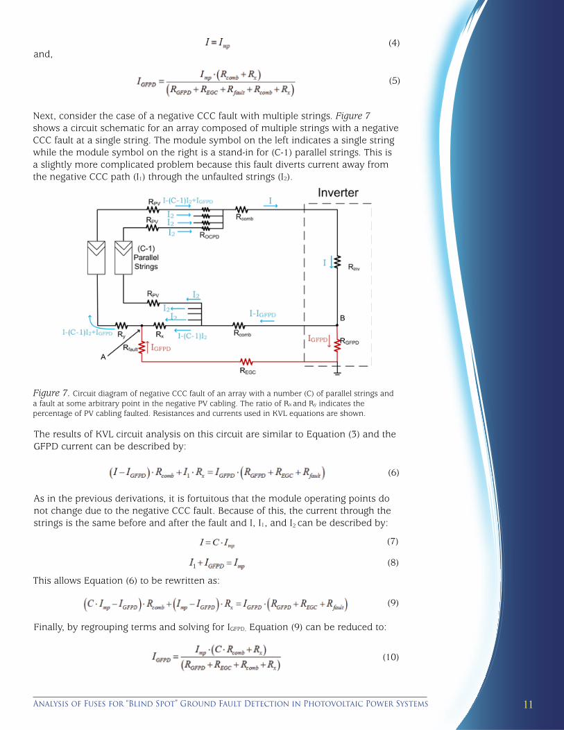
Next, consider the case of a negative CCC fault with multiple strings. Figure 7 shows a circuit schematic for an array composed of multiple strings with a negative CCC fault at a single string. The module symbol on the left indicates a single string while the module symbol on the right is a stand-in for (C-1) parallel strings. This is a slightly more complicated problem because this fault diverts current away from the negative CCC path (I1) through the unfaulted strings (I2).

Figure 7. Circuit diagram of negative CCC fault of an array with a number (C) of parallel strings and a fault at some arbitrary point in the negative PV cabling. The ratio of Rx and Ry indicates the percentage of PV cabling faulted. Resistances and currents used in KVL equations are shown.

The results of KVL circuit analysis on this circuit are similar to Equation (3) and the GFPD current can be described by:

(6)

As in the previous derivations, it is fortuitous that the module operating points do not change due to the negative CCC fault. Because of this, the current through the strings is the same before and after the fault and I, I1, and I2 can be described by:

(7)

(8)

(9)

This allows Equation (6) to be rewritten as:

Finally, by regrouping terms and solving for IGFPD, Equation (9) can be reduced to:

(10)



(12)

(13)

The circuit schematic depicted in Figure 7 is the type of circuit used in the simulations. However, it is usually only representative for <50 string arrays because larger arrays often contain recombiners, shown in Figure 8. Groups of strings are wired together into a combiner box and then recombined before being connected to the inverter.

Figure 8. Circuit diagram of negative CCC fault of an array with a number (C) of multiple parallel strings, which are wired into a combiner box. D combiner boxes outputs are then wired into a recombiner box. A fault occurs at some arbitrary point in the negative PV cabling of a string. The ratio of Rx and Ry indicates the percentage of PV cabling faulted. Resistances and currents used in KVL equations are shown.

In this case, the KVL can be described by:

This equation can be simplified because the strings remain at their maximum power by:

So that Equation (11) can be simplified to:

Finally, the GFPD current can be found by simplifying and grouping to be:

A simple check shows that if the number of combiner boxes per recombiner box is chosen as one or the recombiner resistance is set to zero, Equation (14) reduces to Equation (10).

(14)

(11)

13

(15)

(18)

For the more complicated array shown in Figure 8, there are three possible positions for a fault. The equation for a fault at some point in a string is shown in Equation (14). A fault at the combiner cable means that Rx becomes zero and Rcomb is redefined as Rx and Ry to give a GFPD current of:

This equation is further simplified for the case of a fault at the recombiner cabling. In this case, Rx and Rcomb are both zero in Equation (14) and Rrecomb is redefined as Rx and Ry to give a GFPD current equivalent to:

(16)

The previous circuit analyses have all been carried out for perfect arrays. However, PV arrays have leakage currents. In the case of ground faults at the negative CCC, the leakage current flows in the opposition direction of the fault current (see, for example, Figure 9).

Figure 9. Circuit diagram of negative CCC fault of an array with leakage current. Resistances and currents used in KVL equations are shown.equations are shown.

The KVL analysis of the circuit between points A and B can be described by:

Again, the modules are at maximum power so they can be described by:

So Equation (18) can be inserted into Equation (17):

(17)



(20)

(21)

And solving for Ifault:

The GFPD current is the difference in the fault and leakage currents (and, by convention in these simulations, Ifault is taken to be negative), so Ifault can be trans-formed into IGFPD by:

Finally, Equation (20) can be solved in terms of IGFPD by substituting Equation (21) into Equation (20):

In the simulations, the recombiner topology is not used (D=1, Rrecomb=0 W), so the equation for IGFPD shown as Equation (22) becomes:

(23)

(19)

(22)

15

NUMERICAL SIMULATIONS OF BLIND SPOT FAULTS

As stated before, the analytical solutions assume that the PV modules continue to operate at MPP during the fault. In some situations, (for example, high cable impedance or lengths), some error is introduced. For this reason, computer circuit simulations were used to describe the behavior of PV systems for a wide variety of fault conditions. In the simulations, the PV modules are modeled as non-linear circuits, which are difficult to describe analytically (Zhao, Lehman, de Palma, Mosesian, & Lyons, 2011; Castaner & Silvestre, 2002).

A common method of circuit simulation is SPICE, originally developed at the University of California, Berkeley Electronics Research Laboratory in 1973 (Nagel & Pederson, 1973). SPICE is a general-purpose, open source, analog circuit simulator used to predict circuit behavior. In this work, the program MacSPICE, a derivative of SPICE3f4, was used to analyze the behavior of PV systems in various array configurations and ground fault conditions.

PV Array Simulation Setup

For the purposes of this work, the one-diode model is constructed to approximate a nearly perfect photovoltaic module. The current source is set to supply 2.5 A at short circuit, the diode has an ideality factor of N=80, the shunt resistance is set 1.1020W, and the series resistance is set to 10 m W. This module gives an IV curve with Isc of 2.5 A, Voc of 56 V, and Pmp of 118 W. The MPP has a current of Imp=2.4 A and a voltage of Vmp=49.2 V. These values were chosen to approximate the operation of modules in a 600 V array at Sandia’s Distributed Energy Testing Laboratory on a summer day.

The model of a PV array is composed of a number of strings in parallel (as many as 201). Each string is composed of seven modules in series. Each module is connected to a bypass diode (Isat=4.7.10-12 A, N=1). The array is wired to a resistor, as a basic approximation of the real input impedance of an inverter. The resistance connected to the array in all the simulations is set at the resistance required to generate maximum PV power, Rmp, of the unfaulted array.

The SPICE model was created with the internal resistance of the conductors and GFPD fusing, as shown in Figure 1 in order to investigate ground faults involving the negative CCC. Arrays were simulated with each DC home run cable from the PV to the combiner box totaling 0.25 W (~80 feet of coated copper 12 American wire gauge [AWG] cabling at 3.125 m W/ft). Prior to each string being combined, the positive DC cable is connected to an overcurrent protection device with 0.077 W resistance (4 A KLKD Littelfuse [Littelfuse, 2011] rated for 1.56.Isc). The combiner box is connected to the inverter through cabling with an impedance of 0.00165 W (~50 feet of coated copper 400 circular mil [kcmil] cabling at 0.033 mW/foot). The ground fault is modeled by a resistor connected from the negative CCC to ground through the 0.041 W EGC (determined from field measurements [Ball et al., 2013, in press]). On the faulted string in Figure 3, the PV cabling resistance is split by the fault. This was done so that, by altering the resistance before and after the fault, the position of the fault in the PV cabling could be varied. The value of the inverter resistor is set to the MPP of the unfaulted array. The negative inverter connection is connected to ground through the GFPD.



Simulation Results

To investigate the effect of GFPD resistance on fault current, simulations were carried out for GFPD resistances of 85.5, 22, 8.16, 0.252, 0.124, and 0.0363 W (LittelFuse KLKD resistances for 0.1, 0.25, 0.5, 1, 2, and 5 A fuses [Littelfuse, 2011], respectively) with fault resistances of 0.1, 1, and 25 W. Figure 10 shows the results of the simulations for 1, 2, and 5 A GFPD fuses and fault resistances of 0.1 and 1 W. Simulations with a 1 A (0.252 W), 2 A (0.125 W), and 5 A (0.0363 W) are shown as red, purple, and orange points, respectively. Triangles indicate a fault resistance of 0.1 W while circles represent a 1 W resistance. Solid lines at 1, 2, and 5 A denote the fuse ratings with color corresponding to the fuse trip point. The GFPD current calculated by Equation (18) is denoted by a dashed line for each set of fuse and fault resistances.

Figure 10. Graph of GFPD current vs. array size for various GFPD and fault resistances. The color of the line indicates GFPD resistance. Red traces denote 1 A (0.252 W), while purple and orange traces denote 2 A (0.124 W), and 5 A (0.0363 W), respectively. Only the 1 A and 2 A fuses are sensitive enough to trip due to the blind spot fault. The range in which IGFPD is larger than the trip point is colored in gray.

The GFPD current is linear with the number of strings for all GFPD fuse ratings and fault resistances. Also, for all arrays up to 201 strings, only the 1 A and 2 A GFPDs (at fault resistance of 0.1 W) provide enough GFPD current to trip the fuse (colored regions denote where Ifault>IGFPD). The 1 A GFPD only detects the ground fault in arrays larger than 56 strings while the 2 A GFPD detects faults in arrays larger than 124 strings. The orange traces do not reach 5 A even for 201 strings, so a 5 A GFPD would not trip for a blind spot ground fault of 0.1 or 1 W.

It is tempting to believe that decreasing the fuse rating will increase the number of detectable blind spot faults. However, the decrease in trip point is more than offset by the increased GFPD resistance, so fuses with low ratings will detect fewer blind spots. Figure 11 shows the simulation results for 0.1 (green), 0.25 (purple), and 0.5 A (blue) GFPD fuse ratings at Rfault of 0.1 and 1 W. In each case, due to the increase fuse resistance, the GFPD current is far too small to trip the fuses.

17

Figure 11. Graph of GFPD current vs. array size for various GFPD and fault resistances. The color of the line indicates GFPD resistance. Green traces denote 0.1 A (85.5 W), while purple and blue traces denote 0.25 A (22 W), and 0.5 A (8.16 W), respectively. Even though the fuses have low trip points, due to the increased fuse resistance, the GFPD current is below the fuse trip point and the blind spot window is increased.

Table 1 summarizes the simulation results for GFPD current at different fault resistance and fuse ratings. The color of the cell denotes whether it is possible to detect a blind spot fault. Only the 1 A and 2 A fuses at Rfault=0.1 W have the combination of low trip point and low fuse resistance needed to detect the blind spot fault for large array sizes (more than 56 and 124 strings, respectively). Thus, to limit the size of the blind spot, fuse rating and fuse resistance must both be considered and optimized.

Table 1. GFPD Current for Various Fault Resistances and Fuse Ratings

Fuse (A) Rfault (Ω) IGFPD (A) Minimum Number of Strings to Detect Fault (0.98 kW/string)

0.1 0.0126 A @ 201-string >201 0.1 1 0.019 A @ 201-string >201 25 0.00259 A @ 201-string >201 0.1 0.0486 A @ 201-string >201 0.25 1 0.0446 A @ 201-string >201 25 00608 A @ 201-string >201 0.1 0.0128 A @ 201-string >201 0.5 1 0.0111 A @ 201-string >201 25 0.00862 A @ 201-string >201 0.1 1.00 A @ 56-string 56 1 1 0.727 A @ 201-string >201 25 0.0113 A @ 201-string >201 0.1 2.004 A @ 124-string 124 2 1 0.801 A @ 201-string >201 25 0.0111 A @ 201-string >201 0.1 3.56 A @ 201-string >201 5 1 0.856 A @ 201-string >201 25 0.0113 A @ 201-string >201

Note. The color of the cell indicates if a blind spot fault is detectable. Only the 1 A and 2 A fuses (at Rfault=0.1 W) have both a low enough trip point and a low enough resistance to detect the blind spot fault for array sizes larger than 56 and 124 strings, respectively.



GFPD Current During High-Impedance Blind Spot Ground Faults

Based on the previous results, one may expect that the direction of the GFPD current could indicate blind spot ground faults, but this is not failsafe. Figure 12 shows the GFPD current for 0.1, 0.25, and 0.5 A GFPD fuses for Rfault=25 W. In these simulations, there are two opposing currents through the GFPD: (1) the positive current from the array leakage, and (2) the negative current from the fault. For larger fault resistances, the current through the GFPD does not switch direction for larger arrays because the backfed fault current is smaller than the leakage current for large arrays. In other words, the leakage current per additional string is larger than the fault current per additional string. Figure 12 shows this current contribution per string for module leakage and fault current as a function of fault resistance. For a 1 A GFPD with a 15 W or larger fault, the module leakage increases faster than fault current, so, for larger arrays, the GFPD current will not reverse direction.

Figure 12. (top) Graph of GFPD current vs. array size for fault resistance of 25 W. The direction of the GFPD current will not change at an array size of 105 strings, because for large Rfault values and large array sizes, the leakage current is larger than the fault current. (bottom) Graph of current per string as a function of fault resistance with Ileak=100 mA/module and RGFPD=0.252 W. For fault resistances of more than 15 W, the module leakage is larger than fault current, indicating that, as array size increases, the GFPD current will not reverse.

19

Figure 13 shows the circuit schematic for a 25 W fault resistance for array sizes of one, 101, and 201 strings. For a one-string array, the fault current is a hundred times larger than the leakage current. For a 101-string array, the leakage current and fault currents are approximately equal, so the GFPD current is nearly zero. For a 201-string array, the leakage current is larger than the fault current, and the GFPD current does not reverse direction.

These results indicate that for residential and smaller commercial-scale arrays, it would be possible to detect a blind spot fault by monitoring the direction of GFPD current. To determine the range of fault resistances that could be detected using this technique, simulations were performed for different array sizes varying Rfault. As fault resistance increases, the array size decreases for which there is a GFPD current reversal. Figure 14 shows the value of GFPD current vs. fault resistance for array sizes of eight, 21, 51, 101, and 201 strings with a 0.252 W (1 A) GFPD. The inset shows the crossover points. The fault resistance crossover point for larger array sizes is at a smaller Rfault due to the large amount of leakage current. For example, for an eight-string array, due to the smaller array size, the crossover would be at more than Rfault=110 W, but the 201-string array could only detect the blind spot using a change in GFPD current if the fault is less than about 20 W.



Figure 13. Three circuit schematics illustrating the reversal of GFPD current as array size increases (top). Circuit schematic of a one-string array with Ileak<Ifault (middle), 101-string array with Ileak≈Ifault (bottom), and 201-string array with Ileak>Ifault.

Figure 14. GFPD current as a function of fault resistance for various array sizes. The inset shows the crossover points for each array size.

21

Parametric Study of GFPD Current

As is apparent from Equation (22), the value of GFPD current is dependent on a number of parameters including number of strings (C), combiner cabling resistance (Rcomb), resistance of the faulted section of PV cabling (Rx), GFPD resistance (RGFPD), EGC resistance (REGC), and fault resistance (Rfault). In this section, a study of GFPD current is carried out by varying these system resistances across ranges denoted by Table 2. By determining how GFPD current varies with other parameters, it may be possible for system designers to decrease the blind spot window by maximizing GFPD current.

Table 2. Nominal and High Values of the Parametric Resistances

Parameter Nominal Value (Ω) Low Value (Ω) % Nominal High Value (Ω) % Nominal Rfault -- 0 -- 10 -- RGFPD 0.252 0.01 3.97 100 39,682 REGC 0.041 0.001 2.44 10 24,390 Rx 0.125 (40 ft) 0.002 (0.64 ft) 1.60 10 (3,200 ft) 8,000 Rcomb 0.00165 (50 ft) 1·10-5 (0.30 ft) 0.61 0.3 (9,090 ft) 18,182

Note. A parametric analysis was completed for each parameter for the range of resistances listed above.

Figure 15 shows the results of the parametric analysis for GFPD current as a function of string number (top), and fault resistance (bottom). Figure 16 shows the results of the parametric analysis for GFPD current as a function of EGC resistance (top), and GFPD resistance (bottom) for a 101-string array. The blue line indicates the analytical solution presented in Equation (22) while the black dots indicate the results of the SPICE simulation. The variables used in the simulation are listed in the corresponding graph. There is excellent correlation between the analytical equation and the SPICE simulations for this set of parametric analyses.

Figure 15. Comparison of analytical equation (blue trace) and SPICE simulations (black dots) for GFPD current as a function of other parasitic resistances (top) and GFPD current vs. number of strings in array (bottom). The variables used in the SPICE simulations are listed on each graph. In each set of simulations, the simulation results match the expected analytical solution.



Figure 16: GFPD current vs. EGC resistance (top), and GFPD current as a function of GFPD after resistance (bottom). Green points indicate intrinsic resistance of KLKD “midget” fuses of various sizes from 0.1 to 2 A. The variables used in the SPICE simulations are listed on each graph. In each set of simulations, the simulation results match the expected analytical solution.

Figure 17 (top) shows the parametric test results of GFPD current as a function of the faulted PV cabling resistance (Rx). For the PV cabling resistance, the SPICE simulations follow the analytical solution quite closely for small resistances. However, as the PV cabling resistance increases to values in the multiple ohm range, the simulation results are slightly smaller than expected. This is due to an assumption during the derivation of the analytical equation that each string stays at MPP. While this assumption is true for the majority of resistances, it may not hold true as the cabling resistance increases.

Figure 17 (bottom) shows the array voltage as a function of resistance changes. As the value of Rfault, REGC, and RGFPD change, there is a small impact on the array voltage (less than 0.5 V), so the simulation and analytical results match well. The assumption that each string stays at MPP does not hold as well when Rx changes, so there is a larger effect on the array voltage (black dots and blue crosses). As the value of Rx

approaches 10 W, the faulted string voltage changes by as much as 2 V. This small change in operation voltage is enough to cause the slight GFPD current mismatch between the simulation and analytical solutions.

23

The mismatch between simulation results and the analytical solution is similar for combiner cabling impedance changes (Figure 18). As the combiner cabling impedance increases to an appreciable fraction of the inverter impedance, the assumption that the array stays at MPP before and after the fault is no longer valid (Figure 18, right). This disruptive effect of the cabling impedance on the array voltage is much larger for large arrays because the inverter impedance is so low. This means even for small combiner cabling resistances, the array cannot be assumed to stay at MPP. Because smaller arrays have larger inverter impedances, the assumption holds for much larger cable impedances. As a result, the analytical solution is much closer to the simulation results as the array size decreases (Figure 19).

Figure 17. (top) GFPD current vs. PV cabling resistance of faulted string as determined through calculation of the analytical solution (blue trace) and SPICE simulations (black dots). The results match well for small resistances, but diverge slightly as Rx increases. This is due to the fact that as Rx increases, the operating voltage of the faulted string (bottom) can no longer be assumed to be at Vmp both before and after the fault.



Figure 18. (top) GFPD current as a function of combiner cable resistance. The analytical calculation (blue trace) diverges from the SPICE simulation results as the resistance increases (black dots). This is due to the fact that as the cabling resistance becomes an appreciable function of inverter impedance, the array voltage can no longer be assumed to stay at MPP throughout the fault (bottom). The cabling impedance effect on array voltage is much larger for large arrays because the inverter impedance is so small.

25

Figure 19. As the array size decreases, the analytical solution and SPICE simulation results begin to merge. While the mismatch is large for large array sizes, the mismatch is smaller as the array size goes to 21 strings (top) and is very close for a two-string array (bottom). The analytical and numerical results merge because, as inverter impedance increases, the PV cabling resistance has a much smaller effect on array voltage and the assumption that the array stays at Vmp is more correct.



Summary and conclusions

In this work, analytical and numerical solutions to determine GFPD current for ground fault blind spot cases (where a fault occurs to the grounded CCC) were presented. The results demonstrated the influence of fault and conductor resistances on the detectability of different blind spot ground faults. Blind spot detection is challenging due to the small GFPD current levels and the large influence of fault, GFPD, and cabling resistances on GFPD current. The SPICE model and analytical results were used to determine trends for various ground fault conditions and to ascertain potential benefits of reducing the fuse ratings in PV systems. Decreasing the GFPD ratings to 1 A for large installations would not increase the number of nuisance trips, but would protect against a wider range of ground faults. However, further decreasing the fuse ratings below 1 A does not improve the number of faults that can be detected due to larger internal GFPD resistances and a subsequent decrease in fault current. In fact, because the ground fault fuse resistances increase from 1 A to 0.1 A, more blind spot faults can be detected with the 1 A fuse. Unfortunately, fewer ground faults to other parts of the array can be detected (IEC, 2005), so it is necessary to carefully select the GFPD rating to optimize the types of ground faults that can be detected.

While it may not be possible to provide complete detection for both faults within the array and faults to the grounded CCC using a fuse, the simulations indicate that the detection window for blind spot faults can be optimized by:

1. minimizing leakage current, because fault current is the opposite direction of leakage current and large leakage currents will inhibit the detection of negative CCC faults;

2. decreasing the fuse sizing for large arrays below UL 1741 requirements to 1 A, because module leakage current will be too small to result in nuisance tripping and it will trip on more ground faults;

3. preventing the reduction in fuses below 1 A because the internal resistance of the fuse prevents the fault current from passing through the GFPD;

4. monitoring both GFPD current magnitude and direction (especially for smaller array sizes), because GFPD current can change direction when a fault to the grounded CCC occurs; and

5. employing other fault detection tools such as differential current measurement and insulation monitoring (see [Ball et al., 2013, in press] for more information on alternative ground fault detection techniques and suggestions).

27

ACRONYMS

A ampere

AWG American wire gauge

C number of strings CCC current-carrying conductor

CdTe cadmium telluride

DOE U.S. Department of Energy

EGC equipment grounding conductor

EMI electromagnetic interference

GFDI ground fault detector/interrupter GFPD ground fault protection device

IEC International Electrotechnical Commission IV current voltage

Ileak array leakage current

Imp maximum power current

Isat module diode leakage current

KCL Kirchoff’s Current Law

kcmil circular mil

KVL Kirchoff’s Voltage Law

m2 square meter

MW megaohm

MPP maximum power point

NREL National Renewable Energy Laboratory

W ohm

PARC Palo Alto Research Center

Pmp Power at Maximum Point

PV photovoltaic

Rcomb resistance of combiner cabling

REGC resistance of EGC

Rfault fault resistance

RGFPD GFPD resistance

Rleak leakage current to ground

RPV resistance of PV cabling

Rrecomb recombiner cable resistance

Rx resistance of portion of PV cabling included in fault loop

Ry resistance of portion of PV cabling nots included in fault loop

Solar ABCs Solar America Board for Codes and Standards

SPICE Simulation Program with Integrated Circuit Emphasis

mA microampere

V volts

Vmp voltage at maximum power



REFERENCES

ABB Group. (2010). E 90 range of fuse disconnectors and fuseholders.

Ball, G., Brooks, B., Flicker, J., Johnson, J., Rosenthal, A., Wiles, J. C., & Sherwood, L. (2013 [in press]) Final report: Examination of inverter ground-fault detection “blind spot” with recommendations for mitigation. Solar America Board for Codes and Stan-dards Report.

Brooks, B. (February/March 2011). The bakersfield fire. SolarPro. (4.2), 62-70.

Brooks, B. (January 2012). The ground-fault protection blind spot: Safety concern for larger PV systems in the U.S. Solar America Board for Codes and Standards Report.

Castaner, L. & Silvestre, S. (2002). Modelling photovoltaic systems using PSPICE. Chichester, West Sussex, England: John Wiley and Sons Ltd.

Cooper-Bussmann. (2009). Superior protection for solar power applications. Doc. Num. 3142.

del Cueto, J. A. & McMahon, T. J. (2002). Analysis of leakage currents in photovoltaic modules under high-voltage bias in the field. Progress in Photovoltaics: Research and Applications. Vol. 10 (1), pp. 15-28.

DF Electric. (2012). Photovoltaic fuse-links & fuse holders.

Flicker J., & Johnson, J. (2013). Photovoltaic ground fault and blind spot electrical simulations, Sandia National Laboratories Technical Report.

Hill Technical Sales Group. (2012). Solar PV fuse. Accessed 11.19.2012. http://hilltech.com

International Electrotechnical Commission (IEC). (2005). Crystalline silicon terrestrial photovoltaic (PV) modules-design qualification and type approval. 2nd ed. Geneva, p. 102.

Littelfuse. (November 2011). POWR-GARD fuse datasheet.

Mersen (formerly Ferraz Shawmut). (2010). HP6M(Amp Rating) watts loss data. Newburyport, MA.

Nagel, L. W. & Pederson, D. O. (1973). SPICE (Simulation Program with Integrated Circuit Emphasis). University of California, Berkeley, p. 62.

SIBA Fuses. (2006). URZ-DMI 10x38mm gR 1000 V datasheet. Doc. Num. E19906.

Socomec. (2011-2012). PV fuses. General Catalog 2011-2012.

Underwriters’ Laboratory (UL). (2001). Inverters, converters, controllers, and interconnection system equipment for use with distributed energy resources. UL 1741 ed. Northbrook, IL.

Wiles, J. C. (October 2012). Photovoltaic system grounding. Solar America Board for Codes and Standards Report.

Zhao, Y., Lehman, B., de Palma, J., Mosesian, J., & Lyons, R. (September 1, 2011) Challenges to overcurrent protection devices under line-line faults in solar photovoltaic arrays. Transactions of the IRE Professional Group. 20-27.

http://www.solarabcs.org/about/publications/reports/blindspot/

http://www.solarabcs.org/about/publications/reports/blindspot/

http://www.solarabcs.org/systemgrounding



Solar America Board for Codes and Standardswww.solarabcs.org

Prepared by Jack Flicker Jay Johnson - Solar America … · Prepared by Jack Flicker Jay Johnson...

Documents

Transcript of Prepared by Jack Flicker Jay Johnson - Solar America … · Prepared by Jack Flicker Jay Johnson...