Prepared by Hanadi

 An p ×p Latin Square has p rows and p columns and entries from the first p letters such that each letter appears in every row and in every column.

 

 Latin square design used to eliminate two sources of variability (i.e. allows blocking in two directions).

 

 Advantages:

1 .You can control variation in two Directions .2 .Hopefully you increase efficiency as compared

to the RCBD . 

Disadvantages : The number of levels of each blocking variable

must equal the number of levels of the treatment factor. The Latin square model assumes that there are no interactions between the blocking variables or between the treatment variable and the blocking variable.

The interested model:

pk

pj

pi

y kjikjikji

,...1

,...1

,...1

 The null hypotheses can be considered are:

1 (there is no significant difference in treatment means .

2 (there is no significant difference in row means.

3(there is no significant difference in column means.

 

  Check on assumptions (Normality, Constant variance) perform the ANOVA for the Latin-Square design,

Click through Analyze _ General Linear Model Univariate select dependent variable for the Dependent Variable box. Select row and columns to the Fixed Factor(s) box. click Model in the upper right hand corner.

In that dialogue box put the circle for Custom and then click treatments, row, columns over to the right hand box. In the middle, click the down arrow to Main Effects. click off the arrow in the box labeled Include Intercept in Model. Then hit Continue. For multiple comparisons, click Post Hoc and select the factors for performing multiple comparison procedure, and check on thebox for selecting the method for comparisons (Tukey), and then click Continue and hit OK. 

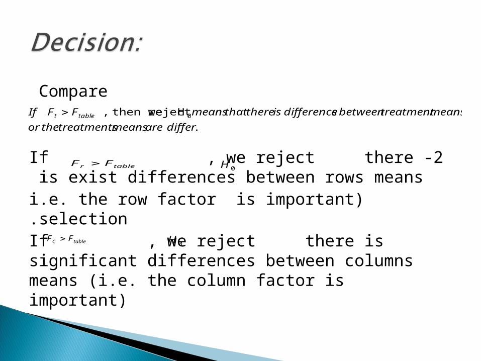
Compare

2 -If , we reject there is exist differences between rows means

)i.e. the row factor is important selection.If , we reject there is significant differences between columns means (i.e. the column factor is important)

.

Hreject then we, 0

differaremeanstreatmentstheor

meanstreatmentbetweensdifferenceistherethatmeansFFIf tablet

tabler FF

tableC FF

0H

0H

If we decide there is no significance difference between rows means or columns means then we can ignore this factor and back to analyze RCBD.

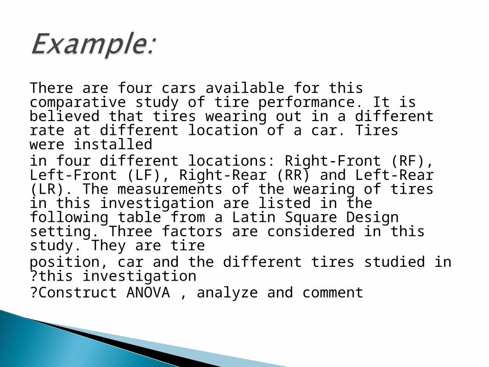
There are four cars available for this comparative study of tire performance. It is believed that tires wearing out in a different rate at different location of a car. Tires were installedin four different locations: Right-Front (RF), Left-Front (LF), Right-Rear (RR) and Left-Rear (LR). The measurements of the wearing of tires in this investigation are listed in the following table from a Latin Square Design setting. Three factors are considered in this study. They are tireposition, car and the different tires studied in this investigation?Construct ANOVA , analyze and comment?

 

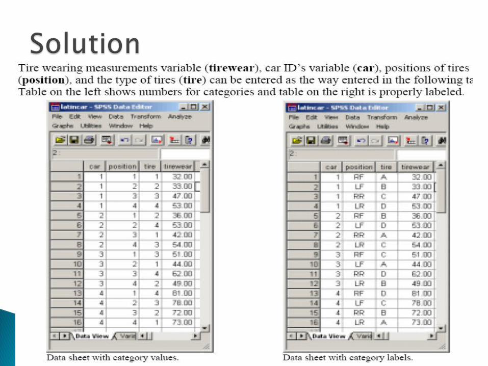
output

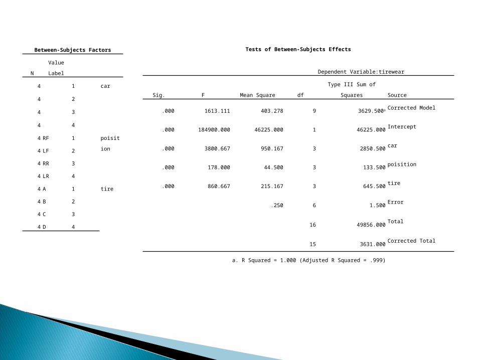
Between-Subjects Factors

Value LabelN

car14

24

34

44

poisition1RF4

2LF4

3RR4

4LR4

tire1A4

2B4

3C4

4D4

Tests of Between-Subjects Effects

Dependent Variable:tirewear

SourceType III Sum of SquaresdfMean SquareFSig.

Corrected Model3629.500a9403.2781613.111.000

Intercept46225.000146225.000184900.000.000

car2850.5003950.1673800.667.000

poisition133.500344.500178.000.000

tire645.5003215.167860.667.000

Error1.5006.250

Total49856.00016

Corrected Total3631.00015

a. R Squared = 1.000 (Adjusted R Squared = .999)

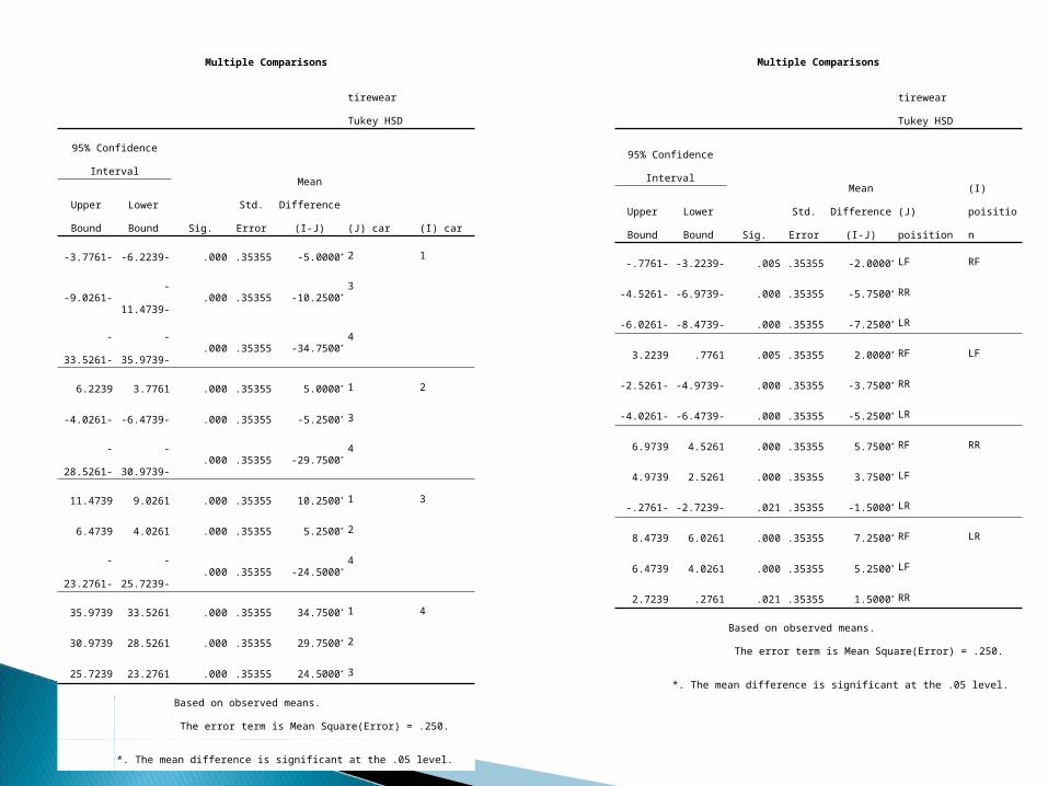
Multiple Comparisons

tirewear

Tukey HSD

(I) car(J) car

Mean

Difference (I-J)Std. ErrorSig.

95% Confidence Interval

Lower

Bound

Upper

Bound

12-5.0000*.35355.000-6.2239--3.7761-

3-10.2500*.35355.000-11.4739--9.0261-

4-34.7500*.35355.000-35.9739--33.5261-

215.0000*.35355.0003.77616.2239

3-5.2500*.35355.000-6.4739--4.0261-

4-29.7500*.35355.000-30.9739--28.5261-

3110.2500*.35355.0009.026111.4739

25.2500*.35355.0004.02616.4739

4-24.5000*.35355.000-25.7239--23.2761-

4134.7500*.35355.00033.526135.9739

229.7500*.35355.00028.526130.9739

324.5000*.35355.00023.276125.7239

Based on observed means.

The error term is Mean Square(Error) = .250.

*. The mean difference is significant at the .05 level.

Multiple Comparisons

tirewear

Tukey HSD

(I) poisition(J) poisition

Mean

Difference (I-J)Std. ErrorSig.

95% Confidence Interval

Lower

Bound

Upper

Bound

RFLF-2.0000*.35355.005-3.2239--.7761-

RR-5.7500*.35355.000-6.9739--4.5261-

LR-7.2500*.35355.000-8.4739--6.0261-

LFRF2.0000*.35355.005.77613.2239

RR-3.7500*.35355.000-4.9739--2.5261-

LR-5.2500*.35355.000-6.4739--4.0261-

RRRF5.7500*.35355.0004.52616.9739

LF3.7500*.35355.0002.52614.9739

LR-1.5000*.35355.021-2.7239--.2761-

LRRF7.2500*.35355.0006.02618.4739

LF5.2500*.35355.0004.02616.4739

RR1.5000*.35355.021.27612.7239

Based on observed means.

The error term is Mean Square(Error) = .250.

*. The mean difference is significant at the .05 level.