Preparation Data Structures 11 graphs
196
Data Structures Graphs Andres Mendez-Vazquez May 8, 2015 1 / 91
-
Upload
andres-mendez-vazquez -
Category
Education
-
view
38 -
download
1
Transcript of Preparation Data Structures 11 graphs
Data StructuresGraphs
Andres Mendez-Vazquez
May 8, 2015
1 / 91

Images/cinvestav-1.jpg
Outline1 Graphs
Graphs EverywhereHistoryBasic Theory
2 Graph RepresentationMatrix RepresentationPossible Code for This RepresentationAdjacency List Representation
3 Traversing the GraphBreadth-first searchDepth-First Search
4 ApplicationsFinding a path between nodesConnected ComponentsSpanning TreesTopological Sorting
2 / 91

Images/cinvestav-1.jpg
Outline1 Graphs
Graphs EverywhereHistoryBasic Theory
2 Graph RepresentationMatrix RepresentationPossible Code for This RepresentationAdjacency List Representation
3 Traversing the GraphBreadth-first searchDepth-First Search
4 ApplicationsFinding a path between nodesConnected ComponentsSpanning TreesTopological Sorting
3 / 91

Images/cinvestav-1.jpg
We are full of Graphs
Maps
4 / 91

Images/cinvestav-1.jpg
We are full of Graphs
State Machines for Branch Prediction in CPU’s
5 / 91

Images/cinvestav-1.jpg
We are full of Graphs
Social Networks
6 / 91

Images/cinvestav-1.jpg
Outline1 Graphs
Graphs EverywhereHistoryBasic Theory
2 Graph RepresentationMatrix RepresentationPossible Code for This RepresentationAdjacency List Representation
3 Traversing the GraphBreadth-first searchDepth-First Search
4 ApplicationsFinding a path between nodesConnected ComponentsSpanning TreesTopological Sorting
7 / 91

Images/cinvestav-1.jpg
History
Something NotableGraph theory started with Euler who was asked to find a nice path acrossthe seven Königsberg bridges
The Actual City
8 / 91

Images/cinvestav-1.jpg
HistorySomething NotableGraph theory started with Euler who was asked to find a nice path acrossthe seven Königsberg bridges
The Actual City
8 / 91

Images/cinvestav-1.jpg
There is No-Solution
Using GraphsThe (Eulerian) path should cross over each of the seven bridges exactlyonce
Can you find Any possible solution?
9 / 91

Images/cinvestav-1.jpg
There is No-Solution
Using GraphsThe (Eulerian) path should cross over each of the seven bridges exactlyonce
Can you find Any possible solution?
9 / 91

Images/cinvestav-1.jpg
Necessary Condition
Euler discovered thatA necessary condition for the walk of the desired form is that the graph beconnected and have exactly zero or two nodes of odd degree.
Add an extra bridge
10 / 91

Images/cinvestav-1.jpg
Necessary Condition
Euler discovered thatA necessary condition for the walk of the desired form is that the graph beconnected and have exactly zero or two nodes of odd degree.
Add an extra bridge
Add Extra Bridge
10 / 91

Images/cinvestav-1.jpg
Studying Graphs
All the previous examples are telling usData Structures are required to design structures to hold the informationcoming from graphs!!!
Good RepresentationsThey will allow to handle the data structures with ease!!!
11 / 91

Images/cinvestav-1.jpg
Studying Graphs
All the previous examples are telling usData Structures are required to design structures to hold the informationcoming from graphs!!!
Good RepresentationsThey will allow to handle the data structures with ease!!!
11 / 91

Images/cinvestav-1.jpg
Outline1 Graphs
Graphs EverywhereHistoryBasic Theory
2 Graph RepresentationMatrix RepresentationPossible Code for This RepresentationAdjacency List Representation
3 Traversing the GraphBreadth-first searchDepth-First Search
4 ApplicationsFinding a path between nodesConnected ComponentsSpanning TreesTopological Sorting
12 / 91

Images/cinvestav-1.jpg
Basic TheoryDefinitionA Graph is composed of the following parts: Nodes and Edges
NodesThey can represent multiple things:
PeopleCitiesStates of Beingetc
EdgesThey can represent multiple things too:
Distance between citiesFriendshipsMatching StringsEtc
13 / 91

Images/cinvestav-1.jpg
Basic TheoryDefinitionA Graph is composed of the following parts: Nodes and Edges
NodesThey can represent multiple things:
PeopleCitiesStates of Beingetc
EdgesThey can represent multiple things too:
Distance between citiesFriendshipsMatching StringsEtc
13 / 91

Images/cinvestav-1.jpg
Basic TheoryDefinitionA Graph is composed of the following parts: Nodes and Edges
NodesThey can represent multiple things:
PeopleCitiesStates of Beingetc
EdgesThey can represent multiple things too:
Distance between citiesFriendshipsMatching StringsEtc
13 / 91

Images/cinvestav-1.jpg
Basic Theory
DefinitionA graph G = (V ,E ) consists of a set of vertices (or nodes) V and a set ofedges E , where we assume that they are finite i.e. |V | = n and |E | = m.
Example
14 / 91

Images/cinvestav-1.jpg
Basic Theory
DefinitionA graph G = (V ,E ) consists of a set of vertices (or nodes) V and a set ofedges E , where we assume that they are finite i.e. |V | = n and |E | = m.
Example
14 / 91

Images/cinvestav-1.jpg
Properties
IncidentAn edge ek = (vi , vj) is incident with the vertices vi and vj .
A simple graph has no self-loops or multiple edges like below
15 / 91

Images/cinvestav-1.jpg
Properties
IncidentAn edge ek = (vi , vj) is incident with the vertices vi and vj .
A simple graph has no self-loops or multiple edges like below
15 / 91

Images/cinvestav-1.jpg
Some properties
DegreeThe degree d(v) of a vertex V is its number of incident edges
A self loopA self-loop counts for 2 in the degree function.
PropositionThe sum of the degrees of a graph G = (V ,E ) equals 2|E | = 2m (trivial).
16 / 91

Images/cinvestav-1.jpg
Some properties
DegreeThe degree d(v) of a vertex V is its number of incident edges
A self loopA self-loop counts for 2 in the degree function.
PropositionThe sum of the degrees of a graph G = (V ,E ) equals 2|E | = 2m (trivial).
16 / 91

Images/cinvestav-1.jpg
Some properties
DegreeThe degree d(v) of a vertex V is its number of incident edges
A self loopA self-loop counts for 2 in the degree function.
PropositionThe sum of the degrees of a graph G = (V ,E ) equals 2|E | = 2m (trivial).
16 / 91

Images/cinvestav-1.jpg
Empty
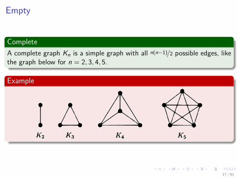
CompleteA complete graph Kn is a simple graph with all n(n−1)/2 possible edges, likethe graph below for n = 2, 3, 4, 5.
Example
17 / 91
Images/cinvestav-1.jpg
Empty
CompleteA complete graph Kn is a simple graph with all n(n−1)/2 possible edges, likethe graph below for n = 2, 3, 4, 5.
Example
17 / 91

Images/cinvestav-1.jpg
We need NICE representations
First OneMatrix Representation
Second OneAdjacency Representation
18 / 91

Images/cinvestav-1.jpg
We need NICE representations
First OneMatrix Representation
Second OneAdjacency Representation
18 / 91

Images/cinvestav-1.jpg
Outline1 Graphs
Graphs EverywhereHistoryBasic Theory
2 Graph RepresentationMatrix RepresentationPossible Code for This RepresentationAdjacency List Representation
3 Traversing the GraphBreadth-first searchDepth-First Search
4 ApplicationsFinding a path between nodesConnected ComponentsSpanning TreesTopological Sorting
19 / 91

Images/cinvestav-1.jpg
Adjacency Matrix Representation
This is the simplest oneIf we number the nodes of an undirected graph:
20 / 91
Images/cinvestav-1.jpg
Adjacency Matrix Representation
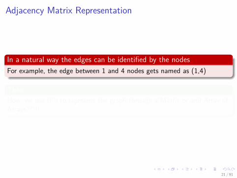
In a natural way the edges can be identified by the nodesFor example, the edge between 1 and 4 nodes gets named as (1,4)
ThenHow, we use this to represent the graph through a Matrix or and Array ofArrays??!!!
21 / 91

Images/cinvestav-1.jpg
Adjacency Matrix Representation
In a natural way the edges can be identified by the nodesFor example, the edge between 1 and 4 nodes gets named as (1,4)
ThenHow, we use this to represent the graph through a Matrix or and Array ofArrays??!!!
21 / 91

Images/cinvestav-1.jpg
What about the following?
How do we indicate that an edge exist given the following matrix1 2 3 4 5 6
1 − − − − − −2 − − − − − −3 − − − − − −4 − − − − − −5 − − − − − −6 − − − − − −
You say it!!Use a 0 for no-edgeUse a 1 for edge
22 / 91

Images/cinvestav-1.jpg
What about the following?
How do we indicate that an edge exist given the following matrix1 2 3 4 5 6
1 − − − − − −2 − − − − − −3 − − − − − −4 − − − − − −5 − − − − − −6 − − − − − −
You say it!!Use a 0 for no-edgeUse a 1 for edge
22 / 91

Images/cinvestav-1.jpg
We have then...
Definition0/1 N × N matrix with N =Number of nodes or verticesA(i , j) = 1 iff (i , j) is an edge
23 / 91

Images/cinvestav-1.jpg
We have then...For the previous example
1 2 3 4 5 61 0 0 0 1 0 02 0 0 0 1 0 03 0 0 0 1 0 04 1 1 1 0 1 05 0 0 0 1 0 16 0 0 0 0 1 0
24 / 91

Images/cinvestav-1.jpg
Properties of the Matrix for Undirected Graphs
Property OneDiagonal entries are zero.
Property TwoAdjacency matrix of an undirected graph is symmetric:
A (i , j) = A (j , i) for all i and j
25 / 91

Images/cinvestav-1.jpg
Properties of the Matrix for Undirected Graphs
Property OneDiagonal entries are zero.
Property TwoAdjacency matrix of an undirected graph is symmetric:
A (i , j) = A (j , i) for all i and j
25 / 91
Images/cinvestav-1.jpg
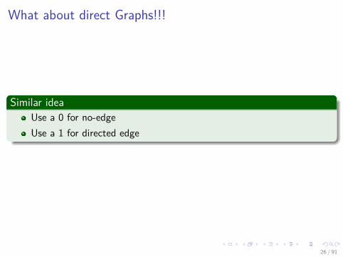
What about direct Graphs!!!
Similar ideaUse a 0 for no-edgeUse a 1 for directed edge
26 / 91
Images/cinvestav-1.jpg
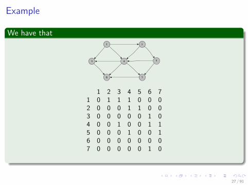
Example
We have that
3
1 2
4 5
6 7
1 2 3 4 5 6 71 0 1 1 1 0 0 02 0 0 0 1 1 0 03 0 0 0 0 0 1 04 0 0 1 0 0 1 15 0 0 0 1 0 0 16 0 0 0 0 0 0 07 0 0 0 0 0 1 0
27 / 91
Images/cinvestav-1.jpg
Outline1 Graphs
Graphs EverywhereHistoryBasic Theory
2 Graph RepresentationMatrix RepresentationPossible Code for This RepresentationAdjacency List Representation
3 Traversing the GraphBreadth-first searchDepth-First Search
4 ApplicationsFinding a path between nodesConnected ComponentsSpanning TreesTopological Sorting
28 / 91

Images/cinvestav-1.jpg
What about the code?Partial Codep u b l i c c l a s s Graph{
// P r i v a t e s t o r a g ep r i v a t e boo l ean a d j a c e n c y M a t r i x [ ] [ ] ;p r i v a t e i n t c e r t e xCount ;
// C o n s t r u c t o rp u b l i c Graph ( i n t ve r t exCount ) {
t h i s . v e r t exCount = ve r t exCount ;a d j a c e n c y M a t r i x = new
boo l ean [ ve r t exCount ] [ v e r t exCount ] ;}
//Some Methodsp u b l i c v o i d addEdge ( i n t i , i n t j ) {
i f ( i >= 0 && i < ve r t exCount && j > 0&& j < ve r t exCount ) {
a d j a c e n c y M a t r i x [ i ] [ j ] = t r u e ;a d j a c e n c y M a t r i x [ j ] [ i ] = t r u e ;}
}p u b l i c v o i d removeEdge ( i n t i , i n t j ) {
i f ( i >= 0 && i < ve r t exCount && j > 0&& j < ve r t exCount ) {
a d j a c e n c y M a t r i x [ i ] [ j ] = f a l s e ;a d j a c e n c y M a t r i x [ j ] [ i ] = f a l s e ;
}}
}
29 / 91

Images/cinvestav-1.jpg
What about Time Complexity?
Operations on a GraphMost of the basic operations in a graph are:
Adding an edge – O(1)
Deleting an edge – O(1)
Answering the question “is there an edge between i and j” – O(1)
Finding the successors of a given vertex – O(N)
Finding (if exists) a path between two vertices – O(N2)
30 / 91
Images/cinvestav-1.jpg
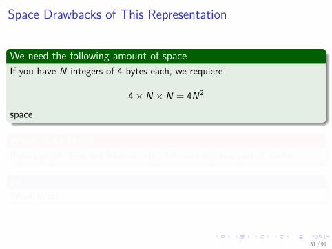
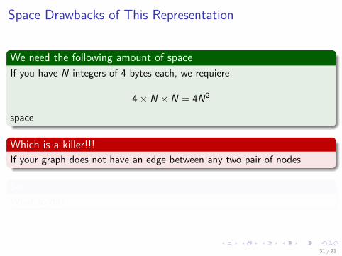
Space Drawbacks of This Representation
We need the following amount of spaceIf you have N integers of 4 bytes each, we requiere
4× N × N = 4N2
space
Which is a killer!!!If your graph does not have an edge between any two pair of nodes
SoWhat to do?
31 / 91
Images/cinvestav-1.jpg
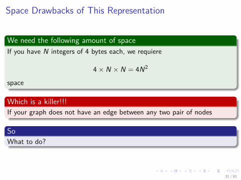
Space Drawbacks of This Representation
We need the following amount of spaceIf you have N integers of 4 bytes each, we requiere
4× N × N = 4N2
space
Which is a killer!!!If your graph does not have an edge between any two pair of nodes
SoWhat to do?
31 / 91
Images/cinvestav-1.jpg
Space Drawbacks of This Representation
We need the following amount of spaceIf you have N integers of 4 bytes each, we requiere
4× N × N = 4N2
space
Which is a killer!!!If your graph does not have an edge between any two pair of nodes
SoWhat to do?
31 / 91

Images/cinvestav-1.jpg
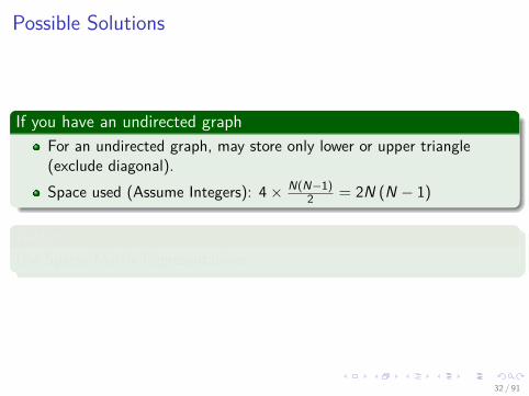
Possible Solutions
If you have an undirected graphFor an undirected graph, may store only lower or upper triangle(exclude diagonal).Space used (Assume Integers): 4× N(N−1)
2 = 2N (N − 1)
BetterUse Sparse Matrix Representations
32 / 91
Images/cinvestav-1.jpg
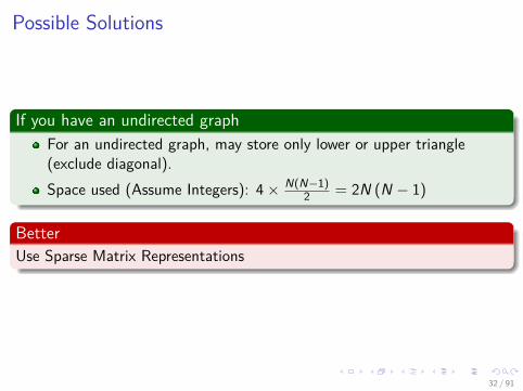
Possible Solutions
If you have an undirected graphFor an undirected graph, may store only lower or upper triangle(exclude diagonal).Space used (Assume Integers): 4× N(N−1)
2 = 2N (N − 1)
BetterUse Sparse Matrix Representations
32 / 91
Images/cinvestav-1.jpg
Possible Solutions
If you have an undirected graphFor an undirected graph, may store only lower or upper triangle(exclude diagonal).Space used (Assume Integers): 4× N(N−1)
2 = 2N (N − 1)
BetterUse Sparse Matrix Representations
32 / 91

Images/cinvestav-1.jpg
We use the sparse Representation of Matrices!!!
Example: Array of Row Chains
33 / 91

Images/cinvestav-1.jpg
We use the sparse Representation of Matrices!!!
Example: Orthogonal Lists
34 / 91

Images/cinvestav-1.jpg
Code For Sparse Representation
Node and Link Representationsp u b l i c c l a s s Node {
p r i v a t e Node next ;p r i v a t e i n t c o l ;
p r i v a t e i n t Value
// Node c o n s t r u c t o rp u b l i c Node ( ){nex t . . .c o l . . .Va lue . . . }// Here the e x t r a// P u b l i c methods. . .
}p u b l i c c l a s s L i n k e d L i s t {
p r i v a t e Node head ;p r i v a t e i n t l i s t C o u n t ;
// L i n k e d L i s t c o n s t r u c t o rp u b l i c L i n k e d L i s t ( ) {head = new Node ( n u l l ) ;l i s t C o u n t = 0 ;}
35 / 91

Images/cinvestav-1.jpg
Code For Sparse Representation
Graph Representationp u b l i c c l a s s G r a p h A d j L i s t S p a r s e {p u b l i c i n t NumNodes ;p u b l i c L i n k L i s t [ ] graph ;
// c o n s t r u c tp u b l i c G r a p h A d j L i s t S p a r s e ( i n t n ) {
NumNodes = n ;graph = new L i n k L i s t [ NumNodes ] ;f o r ( i n t i = 0 ; i < nodes ; i ++)
graph [ i ] = new L i n k L i s t ( ) ;}
// More Methods Here. . .
36 / 91

Images/cinvestav-1.jpg
Outline1 Graphs
Graphs EverywhereHistoryBasic Theory
2 Graph RepresentationMatrix RepresentationPossible Code for This RepresentationAdjacency List Representation
3 Traversing the GraphBreadth-first searchDepth-First Search
4 ApplicationsFinding a path between nodesConnected ComponentsSpanning TreesTopological Sorting
37 / 91

Images/cinvestav-1.jpg
Adjacency List Representation
DefinitionAdjacency list for vertex i is a linear list of vertices adjacent from vertex i .
BasicallyAn array of N adjacency lists.
ThusEach adjacency list is a chain.
38 / 91

Images/cinvestav-1.jpg
Adjacency List Representation
DefinitionAdjacency list for vertex i is a linear list of vertices adjacent from vertex i .
BasicallyAn array of N adjacency lists.
ThusEach adjacency list is a chain.
38 / 91

Images/cinvestav-1.jpg
Adjacency List Representation
DefinitionAdjacency list for vertex i is a linear list of vertices adjacent from vertex i .
BasicallyAn array of N adjacency lists.
ThusEach adjacency list is a chain.
38 / 91

Images/cinvestav-1.jpg
Adjacency List Representation
For the previous example
1
2
3
4
5
6
4
4 6
4
5
1
2
2 3 5
39 / 91
Images/cinvestav-1.jpg
Properties
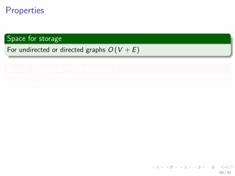
Space for storageFor undirected or directed graphs O (V + E )
Search: Successful or UnsuccessfulO(1 + degree(v))
In additionAdjacency lists can readily be adapted to represent weighted graphs
Weight function w : E → RThe weight w(u, v) of the edge (u, v) ∈ E is simply stored withvertex v in u’s adjacency list
40 / 91

Images/cinvestav-1.jpg
Properties
Space for storageFor undirected or directed graphs O (V + E )
Search: Successful or UnsuccessfulO(1 + degree(v))
In additionAdjacency lists can readily be adapted to represent weighted graphs
Weight function w : E → RThe weight w(u, v) of the edge (u, v) ∈ E is simply stored withvertex v in u’s adjacency list
40 / 91

Images/cinvestav-1.jpg
Possible Disadvantage
When looking to see if an edge existThere is no quicker way to determine if a given edge (u,v)
41 / 91

Images/cinvestav-1.jpg
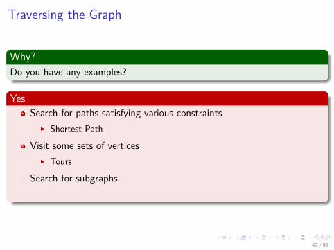
Traversing the Graph
Why?Do you have any examples?
YesSearch for paths satisfying various constraints
I Shortest Path
Visit some sets of verticesI Tours
Search for subgraphsI Isomorphisms
42 / 91

Images/cinvestav-1.jpg
Traversing the Graph
Why?Do you have any examples?
YesSearch for paths satisfying various constraints
I Shortest Path
Visit some sets of verticesI Tours
Search for subgraphsI Isomorphisms
42 / 91

Images/cinvestav-1.jpg
Traversing the Graph
Why?Do you have any examples?
YesSearch for paths satisfying various constraints
I Shortest Path
Visit some sets of verticesI Tours
Search for subgraphsI Isomorphisms
42 / 91

Images/cinvestav-1.jpg
Traversing the Graph
Why?Do you have any examples?
YesSearch for paths satisfying various constraints
I Shortest Path
Visit some sets of verticesI Tours
Search for subgraphsI Isomorphisms
42 / 91
Images/cinvestav-1.jpg
Traversing the Graph
Why?Do you have any examples?
YesSearch for paths satisfying various constraints
I Shortest Path
Visit some sets of verticesI Tours
Search for subgraphsI Isomorphisms
42 / 91

Images/cinvestav-1.jpg
Traversing the Graph
Why?Do you have any examples?
YesSearch for paths satisfying various constraints
I Shortest Path
Visit some sets of verticesI Tours
Search for subgraphsI Isomorphisms
42 / 91

Images/cinvestav-1.jpg
Traversing the Graph
Why?Do you have any examples?
YesSearch for paths satisfying various constraints
I Shortest Path
Visit some sets of verticesI Tours
Search for subgraphsI Isomorphisms
42 / 91

Images/cinvestav-1.jpg
Outline1 Graphs
Graphs EverywhereHistoryBasic Theory
2 Graph RepresentationMatrix RepresentationPossible Code for This RepresentationAdjacency List Representation
3 Traversing the GraphBreadth-first searchDepth-First Search
4 ApplicationsFinding a path between nodesConnected ComponentsSpanning TreesTopological Sorting
43 / 91

Images/cinvestav-1.jpg
Breadth-first search
DefinitionGiven a graph G = (V ,E ) and a source vertex s, breadth-first searchsystematically explores the edges of Gto “discover” every vertex that isreachable from the vertex s
Something NotableA vertex is discovered the first time it is encountered during the search
44 / 91

Images/cinvestav-1.jpg
Defining Some Basic Terms
ColorGiven a node u, we have that
I color is a field indicatingF WHITE Never visited nodeF GRAY Node pointer is at the Queue QF BLACK Node has been visited and processed
45 / 91

Images/cinvestav-1.jpg
Defining Some Basic Terms
ColorGiven a node u, we have that
I color is a field indicatingF WHITE Never visited nodeF GRAY Node pointer is at the Queue QF BLACK Node has been visited and processed
45 / 91

Images/cinvestav-1.jpg
Defining Some Basic Terms
ColorGiven a node u, we have that
I color is a field indicatingF WHITE Never visited nodeF GRAY Node pointer is at the Queue QF BLACK Node has been visited and processed
45 / 91

Images/cinvestav-1.jpg
Defining Some Basic Terms
ColorGiven a node u, we have that
I color is a field indicatingF WHITE Never visited nodeF GRAY Node pointer is at the Queue QF BLACK Node has been visited and processed
45 / 91

Images/cinvestav-1.jpg
Defining Some Basic Terms
ColorGiven a node u, we have that
I color is a field indicatingF WHITE Never visited nodeF GRAY Node pointer is at the Queue QF BLACK Node has been visited and processed
45 / 91

Images/cinvestav-1.jpg
Defining Some Basic Terms
Distance dGiven a node u, we have that
I d is a field indicating the distance from the node source s so far
46 / 91

Images/cinvestav-1.jpg
Defining Some Basic Terms
Predecesor π
Given a node u, we have thatI π is a field indicating who is the immediate predecessor of u in the
path from s to u
47 / 91

Images/cinvestav-1.jpg
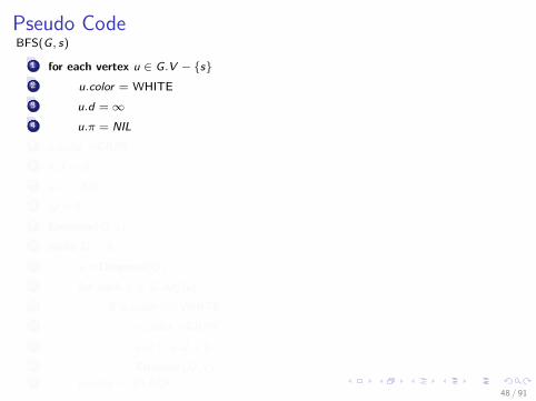
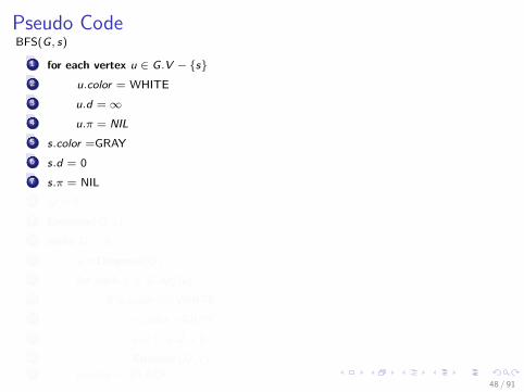
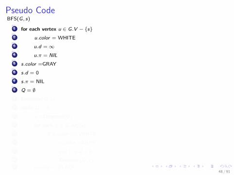
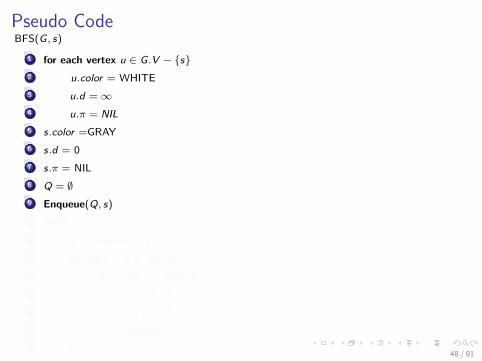
Pseudo CodeBFS(G, s)
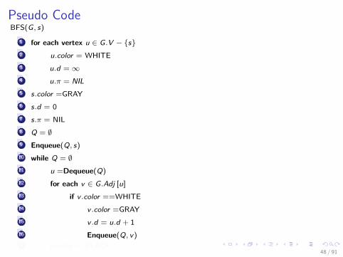
1 for each vertex u ∈ G.V − {s}2 u.color = WHITE3 u.d =∞4 u.π = NIL5 s.color =GRAY6 s.d = 07 s.π = NIL8 Q = ∅9 Enqueue(Q, s)10 while Q = ∅11 u =Dequeue(Q)
12 for each v ∈ G.Adj [u]13 if v .color ==WHITE14 v .color =GRAY15 v .d = u.d + 116 Enqueue(Q, v)17 u.color = BLACK
48 / 91

Images/cinvestav-1.jpg
Pseudo CodeBFS(G, s)
1 for each vertex u ∈ G.V − {s}2 u.color = WHITE3 u.d =∞4 u.π = NIL5 s.color =GRAY6 s.d = 07 s.π = NIL8 Q = ∅9 Enqueue(Q, s)10 while Q = ∅11 u =Dequeue(Q)
12 for each v ∈ G.Adj [u]13 if v .color ==WHITE14 v .color =GRAY15 v .d = u.d + 116 Enqueue(Q, v)17 u.color = BLACK
48 / 91
Images/cinvestav-1.jpg
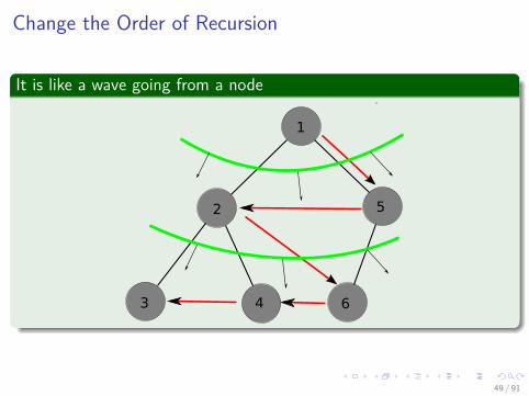
Change the Order of Recursion
It is like a wave going from a node
1
2
3 4
5
6
49 / 91

Images/cinvestav-1.jpg
Example
What do you see?
50 / 91

Images/cinvestav-1.jpg
Example
What do you see?
51 / 91

Images/cinvestav-1.jpg
Example
What do you see?
52 / 91

Images/cinvestav-1.jpg
Example
What do you see?
53 / 91

Images/cinvestav-1.jpg
Example
What do you see?
54 / 91

Images/cinvestav-1.jpg
Example
What do you see?
55 / 91

Images/cinvestav-1.jpg
Example
What do you see?
56 / 91

Images/cinvestav-1.jpg
Example
What do you see?
57 / 91

Images/cinvestav-1.jpg
Complexity
What about the outer loop?O(V ) Enqueue / Dequeue operations – Each adjacency list is processedonly once.
What about the inner loop?The sum of the lengths of f all the adjacency lists is Θ(E ) so the scanningtakes O(E )
58 / 91

Images/cinvestav-1.jpg
Complexity
What about the outer loop?O(V ) Enqueue / Dequeue operations – Each adjacency list is processedonly once.
What about the inner loop?The sum of the lengths of f all the adjacency lists is Θ(E ) so the scanningtakes O(E )
58 / 91

Images/cinvestav-1.jpg
Complexity
Overhead of CreationO (V )
ThenTotal complexity O (V + E )
59 / 91

Images/cinvestav-1.jpg
Complexity
Overhead of CreationO (V )
ThenTotal complexity O (V + E )
59 / 91
Images/cinvestav-1.jpg
Properties
Something NotableBreadth-first search constructs a breadth-first tree, initially containing onlyits root, which is the source vertex s
ThusWe say that u is the predecessor or parent of v in the breadth-first tree.
60 / 91

Images/cinvestav-1.jpg
Properties
Something NotableBreadth-first search constructs a breadth-first tree, initially containing onlyits root, which is the source vertex s
ThusWe say that u is the predecessor or parent of v in the breadth-first tree.
60 / 91
Images/cinvestav-1.jpg
Breadth-First Search Property
Something NotableAll vertices reachable from the start vertex (including the start vertex) arevisited.
61 / 91

Images/cinvestav-1.jpg
Outline1 Graphs
Graphs EverywhereHistoryBasic Theory
2 Graph RepresentationMatrix RepresentationPossible Code for This RepresentationAdjacency List Representation
3 Traversing the GraphBreadth-first searchDepth-First Search
4 ApplicationsFinding a path between nodesConnected ComponentsSpanning TreesTopological Sorting
62 / 91
Images/cinvestav-1.jpg
Depth-first search
Given GPick an unvisited vertex v, remember the rest.
I Recurse on vertices adjacent to v
63 / 91

Images/cinvestav-1.jpg
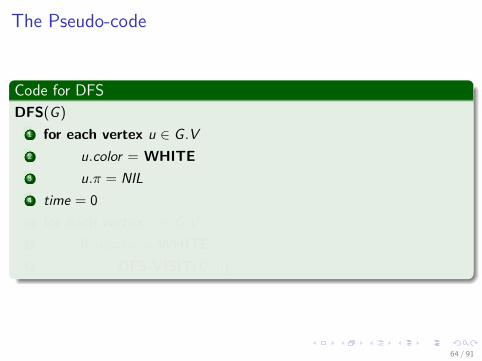
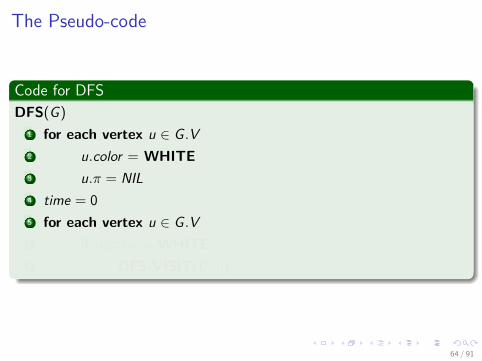
The Pseudo-code
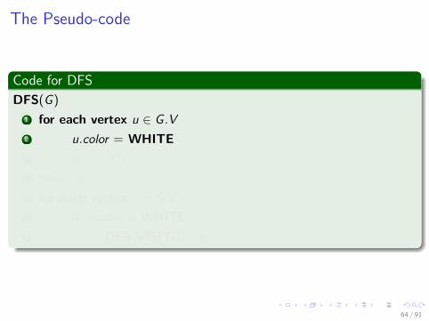
Code for DFSDFS(G)
1 for each vertex u ∈ G .V2 u.color = WHITE3 u.π = NIL4 time = 05 for each vertex u ∈ G .V6 if u.color = WHITE7 DFS-VISIT(G , u)
64 / 91
Images/cinvestav-1.jpg
The Pseudo-code
Code for DFSDFS(G)
1 for each vertex u ∈ G .V2 u.color = WHITE3 u.π = NIL4 time = 05 for each vertex u ∈ G .V6 if u.color = WHITE7 DFS-VISIT(G , u)
64 / 91

Images/cinvestav-1.jpg
The Pseudo-code
Code for DFSDFS(G)
1 for each vertex u ∈ G .V2 u.color = WHITE3 u.π = NIL4 time = 05 for each vertex u ∈ G .V6 if u.color = WHITE7 DFS-VISIT(G , u)
64 / 91
Images/cinvestav-1.jpg
The Pseudo-code
Code for DFSDFS(G)
1 for each vertex u ∈ G .V2 u.color = WHITE3 u.π = NIL4 time = 05 for each vertex u ∈ G .V6 if u.color = WHITE7 DFS-VISIT(G , u)
64 / 91
Images/cinvestav-1.jpg
The Pseudo-code
Code for DFSDFS(G)
1 for each vertex u ∈ G .V2 u.color = WHITE3 u.π = NIL4 time = 05 for each vertex u ∈ G .V6 if u.color = WHITE7 DFS-VISIT(G , u)
64 / 91

Images/cinvestav-1.jpg
The Pseudo-code
Code for DFSDFS(G)
1 for each vertex u ∈ G .V2 u.color = WHITE3 u.π = NIL4 time = 05 for each vertex u ∈ G .V6 if u.color = WHITE7 DFS-VISIT(G , u)
64 / 91

Images/cinvestav-1.jpg
The Pseudo-code
Code for DFSDFS(G)
1 for each vertex u ∈ G .V2 u.color = WHITE3 u.π = NIL4 time = 05 for each vertex u ∈ G .V6 if u.color = WHITE7 DFS-VISIT(G , u)
64 / 91

Images/cinvestav-1.jpg
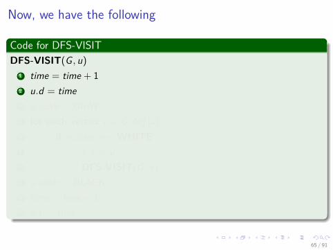
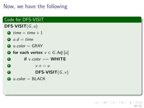
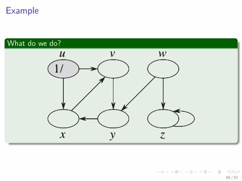
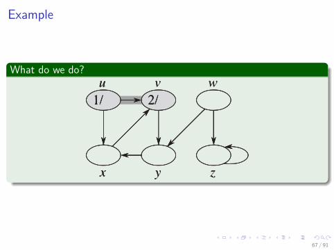
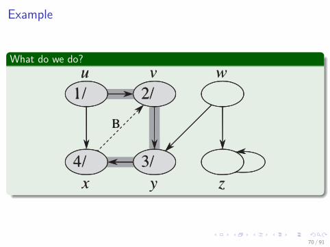
Now, we have the following
Code for DFS-VISITDFS-VISIT(G , u)
1 time = time + 12 u.d = time3 u.color = GRAY4 for each vertex v ∈ G .Adj [u]
5 if v .color == WHITE6 v .π = u7 DFS-VISIT(G , v)
8 u.color = BLACK9 time = time + 110 u.f = time
65 / 91
Images/cinvestav-1.jpg
Now, we have the following
Code for DFS-VISITDFS-VISIT(G , u)
1 time = time + 12 u.d = time3 u.color = GRAY4 for each vertex v ∈ G .Adj [u]
5 if v .color == WHITE6 v .π = u7 DFS-VISIT(G , v)
8 u.color = BLACK9 time = time + 110 u.f = time
65 / 91

Images/cinvestav-1.jpg
Now, we have the following
Code for DFS-VISITDFS-VISIT(G , u)
1 time = time + 12 u.d = time3 u.color = GRAY4 for each vertex v ∈ G .Adj [u]
5 if v .color == WHITE6 v .π = u7 DFS-VISIT(G , v)
8 u.color = BLACK9 time = time + 110 u.f = time
65 / 91

Images/cinvestav-1.jpg
Now, we have the following
Code for DFS-VISITDFS-VISIT(G , u)
1 time = time + 12 u.d = time3 u.color = GRAY4 for each vertex v ∈ G .Adj [u]
5 if v .color == WHITE6 v .π = u7 DFS-VISIT(G , v)
8 u.color = BLACK9 time = time + 110 u.f = time
65 / 91

Images/cinvestav-1.jpg
Now, we have the following
Code for DFS-VISITDFS-VISIT(G , u)
1 time = time + 12 u.d = time3 u.color = GRAY4 for each vertex v ∈ G .Adj [u]
5 if v .color == WHITE6 v .π = u7 DFS-VISIT(G , v)
8 u.color = BLACK9 time = time + 110 u.f = time
65 / 91

Images/cinvestav-1.jpg
Now, we have the following
Code for DFS-VISITDFS-VISIT(G , u)
1 time = time + 12 u.d = time3 u.color = GRAY4 for each vertex v ∈ G .Adj [u]
5 if v .color == WHITE6 v .π = u7 DFS-VISIT(G , v)
8 u.color = BLACK9 time = time + 110 u.f = time
65 / 91

Images/cinvestav-1.jpg
Now, we have the following
Code for DFS-VISITDFS-VISIT(G , u)
1 time = time + 12 u.d = time3 u.color = GRAY4 for each vertex v ∈ G .Adj [u]
5 if v .color == WHITE6 v .π = u7 DFS-VISIT(G , v)
8 u.color = BLACK9 time = time + 110 u.f = time
65 / 91
Images/cinvestav-1.jpg
Now, we have the following
Code for DFS-VISITDFS-VISIT(G , u)
1 time = time + 12 u.d = time3 u.color = GRAY4 for each vertex v ∈ G .Adj [u]
5 if v .color == WHITE6 v .π = u7 DFS-VISIT(G , v)
8 u.color = BLACK9 time = time + 110 u.f = time
65 / 91

Images/cinvestav-1.jpg
Now, we have the following
Code for DFS-VISITDFS-VISIT(G , u)
1 time = time + 12 u.d = time3 u.color = GRAY4 for each vertex v ∈ G .Adj [u]
5 if v .color == WHITE6 v .π = u7 DFS-VISIT(G , v)
8 u.color = BLACK9 time = time + 110 u.f = time
65 / 91

Images/cinvestav-1.jpg
Now, we have the following
Code for DFS-VISITDFS-VISIT(G , u)
1 time = time + 12 u.d = time3 u.color = GRAY4 for each vertex v ∈ G .Adj [u]
5 if v .color == WHITE6 v .π = u7 DFS-VISIT(G , v)
8 u.color = BLACK9 time = time + 110 u.f = time
65 / 91
Images/cinvestav-1.jpg
Example
What do we do?
66 / 91
Images/cinvestav-1.jpg
Example
What do we do?
67 / 91

Images/cinvestav-1.jpg
Example
What do we do?
68 / 91

Images/cinvestav-1.jpg
Example
What do we do?
69 / 91
Images/cinvestav-1.jpg
Example
What do we do?
70 / 91

Images/cinvestav-1.jpg
Example
What do we do?
71 / 91

Images/cinvestav-1.jpg
Example
What do we do?
72 / 91

Images/cinvestav-1.jpg
Example
What do we do?
73 / 91

Images/cinvestav-1.jpg
Complexity
Analysis1 The loops on lines 1–3 and lines 5–7 of DFS take Θ (V ).2 The procedure DFS-VISIT is called exactly once for each vertex
v ∈ V .3 During an execution of DFS-VISIT(G , v) the loop on lines 4–7
executes |Adj (v)| times.4 But
∑v∈V |Adj (v)| = O (E ) we have that the cost of executing g
lines 4–7 of DFS-VISIT is Θ (E ) .
ThenDFS complexity is Θ (V + E )
74 / 91

Images/cinvestav-1.jpg
Applications
We have severalFinding a path between nodesStrongly Connected ComponentsSpanning TreesTopological Sort - The Program (or Project) Evaluation and Review(PERT)Computer Vision AlgorithmsArtificial Intelligence AlgorithmsImportance in Social NetworkRank Algorithms for GoogleEtc.
75 / 91

Images/cinvestav-1.jpg
Outline1 Graphs
Graphs EverywhereHistoryBasic Theory
2 Graph RepresentationMatrix RepresentationPossible Code for This RepresentationAdjacency List Representation
3 Traversing the GraphBreadth-first searchDepth-First Search
4 ApplicationsFinding a path between nodesConnected ComponentsSpanning TreesTopological Sorting
76 / 91

Images/cinvestav-1.jpg
Finding a path between nodes
We do the followingStart a breadth-first search at vertex v .Terminate when vertex u is visited or when Q becomes empty(whichever occurs first).
Time ComplexityO(V 2)when adjacency matrix used.
O(V + E ) when adjacency lists used.
77 / 91

Images/cinvestav-1.jpg
Finding a path between nodes
We do the followingStart a breadth-first search at vertex v .Terminate when vertex u is visited or when Q becomes empty(whichever occurs first).
Time ComplexityO(V 2)when adjacency matrix used.
O(V + E ) when adjacency lists used.
77 / 91

Images/cinvestav-1.jpg
Finding a path between nodes
We do the followingStart a breadth-first search at vertex v .Terminate when vertex u is visited or when Q becomes empty(whichever occurs first).
Time ComplexityO(V 2)when adjacency matrix used.
O(V + E ) when adjacency lists used.
77 / 91
Images/cinvestav-1.jpg
Finding a path between nodes
We do the followingStart a breadth-first search at vertex v .Terminate when vertex u is visited or when Q becomes empty(whichever occurs first).
Time ComplexityO(V 2)when adjacency matrix used.
O(V + E ) when adjacency lists used.
77 / 91

Images/cinvestav-1.jpg
This allow to use the Algorithm for finding The ShortestPath
ClearlyThis is the unweighted version or all weights are equal!!!
We have the following functionδ (s, v)= shortest path from s to v
We claim thatUpon termination of BFS, every vertex v ∈ V reachable from s hasdistance(v) = δ(s, v)
78 / 91

Images/cinvestav-1.jpg
Outline1 Graphs
Graphs EverywhereHistoryBasic Theory
2 Graph RepresentationMatrix RepresentationPossible Code for This RepresentationAdjacency List Representation
3 Traversing the GraphBreadth-first searchDepth-First Search
4 ApplicationsFinding a path between nodesConnected ComponentsSpanning TreesTopological Sorting
79 / 91

Images/cinvestav-1.jpg
Connected Components
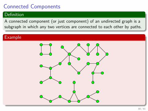
DefinitionA connected component (or just component) of an undirected graph is asubgraph in which any two vertices are connected to each other by paths.
Example
80 / 91
Images/cinvestav-1.jpg
Connected ComponentsDefinitionA connected component (or just component) of an undirected graph is asubgraph in which any two vertices are connected to each other by paths.
Example
80 / 91

Images/cinvestav-1.jpg
Procedure
FirstStart a breadth-first search at any as yet unvisited vertex of the graph.
ThusNewly visited vertices (plus edges between them) define a component.
RepeatRepeat until all vertices are visited.
81 / 91

Images/cinvestav-1.jpg
Procedure
FirstStart a breadth-first search at any as yet unvisited vertex of the graph.
ThusNewly visited vertices (plus edges between them) define a component.
RepeatRepeat until all vertices are visited.
81 / 91
Images/cinvestav-1.jpg
Procedure
FirstStart a breadth-first search at any as yet unvisited vertex of the graph.
ThusNewly visited vertices (plus edges between them) define a component.
RepeatRepeat until all vertices are visited.
81 / 91

Images/cinvestav-1.jpg
Time
O (V 2)
When adjacency matrix used
O(V + E )
When adjacency lists used (E is number of edges)
82 / 91

Images/cinvestav-1.jpg
Time
O (V 2)
When adjacency matrix used
O(V + E )
When adjacency lists used (E is number of edges)
82 / 91

Images/cinvestav-1.jpg
Outline1 Graphs
Graphs EverywhereHistoryBasic Theory
2 Graph RepresentationMatrix RepresentationPossible Code for This RepresentationAdjacency List Representation
3 Traversing the GraphBreadth-first searchDepth-First Search
4 ApplicationsFinding a path between nodesConnected ComponentsSpanning TreesTopological Sorting
83 / 91
Images/cinvestav-1.jpg
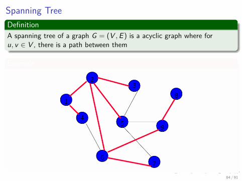
Spanning TreeDefinitionA spanning tree of a graph G = (V ,E ) is a acyclic graph where foru, v ∈ V , there is a path between them
Example
84 / 91

Images/cinvestav-1.jpg
Spanning TreeDefinitionA spanning tree of a graph G = (V ,E ) is a acyclic graph where foru, v ∈ V , there is a path between them
Example
84 / 91

Images/cinvestav-1.jpg
Procedure
FirstStart a breadth-first search at any vertex of the graph.
ThusIf graph is connected, the n − 1 edges used to get to unvisited verticesdefine a spanning tree (breadth-first spanning tree).
85 / 91

Images/cinvestav-1.jpg
Procedure
FirstStart a breadth-first search at any vertex of the graph.
ThusIf graph is connected, the n − 1 edges used to get to unvisited verticesdefine a spanning tree (breadth-first spanning tree).
85 / 91

Images/cinvestav-1.jpg
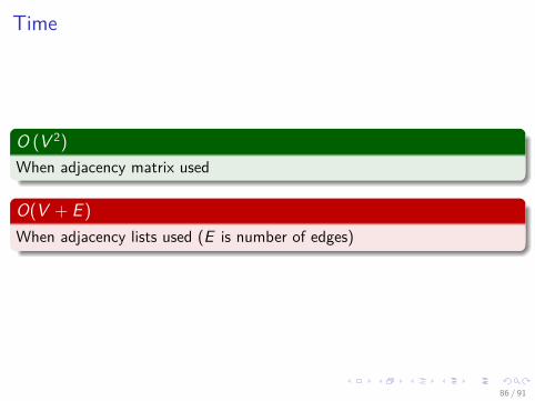
Time
O (V 2)
When adjacency matrix used
O(V + E )
When adjacency lists used (E is number of edges)
86 / 91
Images/cinvestav-1.jpg
Time
O (V 2)
When adjacency matrix used
O(V + E )
When adjacency lists used (E is number of edges)
86 / 91

Images/cinvestav-1.jpg
Outline1 Graphs
Graphs EverywhereHistoryBasic Theory
2 Graph RepresentationMatrix RepresentationPossible Code for This RepresentationAdjacency List Representation
3 Traversing the GraphBreadth-first searchDepth-First Search
4 ApplicationsFinding a path between nodesConnected ComponentsSpanning TreesTopological Sorting
87 / 91

Images/cinvestav-1.jpg
Topological Sorting
DefinitionsA topological sort (sometimes abbreviated topsort or toposort) ortopological ordering of a directed graph is a linear ordering of its verticessuch that for every directed edge (u, v) from vertex u to vertex y , u comesbefore v in the ordering.
From Industrial EngineeringThe canonical application of topological sorting (topological order) isin scheduling a sequence of jobs or tasks based on their dependencies.Topological sorting algorithms were first studied in the early 1960s inthe context of the PERT technique for scheduling in projectmanagement (Jarnagin 1960).
88 / 91

Images/cinvestav-1.jpg
Then
We have thatThe jobs are represented by vertices, and there is an edge from x to y ifjob x must be completed before job y can be started.
ExampleWhen washing clothes, the washing machine must finish before we put theclothes to dry.
ThenA topological sort gives an order in which to perform the jobs.
89 / 91

Images/cinvestav-1.jpg
Algorithm
Pseudo CodeTOPOLOGICAL-SORT
1 Call DFS(G) to compute finishing times v .f for each vertex v .2 As each vertex is finished, insert it onto the front of a linked list3 Return the linked list of vertices
90 / 91

Images/cinvestav-1.jpg
Algorithm
Pseudo CodeTOPOLOGICAL-SORT
1 Call DFS(G) to compute finishing times v .f for each vertex v .2 As each vertex is finished, insert it onto the front of a linked list3 Return the linked list of vertices
90 / 91

Images/cinvestav-1.jpg
Algorithm
Pseudo CodeTOPOLOGICAL-SORT
1 Call DFS(G) to compute finishing times v .f for each vertex v .2 As each vertex is finished, insert it onto the front of a linked list3 Return the linked list of vertices
90 / 91

Images/cinvestav-1.jpg
Algorithm
Pseudo CodeTOPOLOGICAL-SORT
1 Call DFS(G) to compute finishing times v .f for each vertex v .2 As each vertex is finished, insert it onto the front of a linked list3 Return the linked list of vertices
90 / 91

Images/cinvestav-1.jpg
Example
Dressing
91 / 91