N A S A C O N T R A C T O R

R E P O R T

N A S A C R - 2 7 5 9

01I

PRELIMINARY STUDY OF CONTAMINANT

PARTICULATES AROUND SKYLAB

D. W. Sch tier man and J. L. Weinberg

Prepared by

STATE UNIVERSITY OF NEW YORK AT ALBANY

Albany, N.Y. 12203

Jor George C. Marshall Space Flight Center

NATIONAL A E R O N A U T I C S AND SPACE ADMINISTRATION • WASHINGTON, D. C. • OCTOBER 1976

https://ntrs.nasa.gov/search.jsp?R=19770004032 2018-03-21T19:02:56+00:00Z

1. Report No.NASA CP-2759

2. Government Accession No.

4. Title and Subtitle

D r e l in i ina ry Study of Contaminant Particulates around Skylab

7. Author(s)

D. \V. Schuerman and '. L. Weinberg

9. Performing Organization Name and Address

Space Astronomy LaboratoryState University of New York at AlbanyAlbany. New York 12203

12. Sponsoring Agency Name and Address

National Aeronautics and Space AdministrationWashington, D. C. 20546

3. Recipient's Catalog No.

5. Report Date

October 19766. Performing Organization Code

8. Performing Organization Report No.

M-lsT

10. Work Unit No.

11. Contract or Grant No.

NASS-31902

13. Type of Report and Period Covered

Contractor

14. Sponsoring Agency Code

15. Supplementary Notes

•

16. AbstractTechniques originally developed for the Skylab T025 contamination experiment were applied to S052

white-light coronagraph data in a preliminary study to investigate particulates around Skylab. Periods wereselected which contained some contamination, even though there were no apparent dumps or vents duringthese periods. For the first t ime, velocity and size distributions were determined from optical data forparticles within 200 meters of the spacecraft. Foth photographic ( f i l particle tracks) and video (34 particles)observations yield an upper l imi t on particle radius of 100/jm. The smallest particle observed had a radiusof 5 pm. but this l imit is imposed by the sensitivity of the coronagraph and does not reflect a true lower cutoffof the size distribution. The typical particle velocity as determined from the video data was 1 m/s. Thenumber density of particulates within 200 meters of the spacecraft was found to vary from approximately10~Vcm3 to 2 X 10"Vcm3 (from 5 to 100 particles per field of view).

Selected photometric data from the SO^S zodiacal light experiment during mission SL-2 were alsoexamined for evidence of contamination. Contrary to the results of an analysis of these same data by Muscariand Jambor (Skylab experiment T027) , we find no evidence for a detectable spacecraft corona. Although thephotometer data were taken at different times, this result is consistent with the S052 analysis which finds thetypical number density of particles larger than 5 pm to be at or below the photometer's 1 to 3 S 1 0 (V) columnbrightness threshold for detection.1 Since particles smaller than 5 pm are expected to be present, the brightnessof the spacecraft corona should be even brighter than that predicted by the S052 data.

This study demonstrates the need for further joint observations and correlative studies of singleparticle data as obtained from an imaging system and particle cloud data obtained from a photometer system:this would make possible an accurate prediction of the effect on one from the results of the other and a morecomplete description of the contaminant cloud.

'Equivalent number of 10th magnitude solar (G2V) stars per square degree at mean solar distance. At5300 A , 1 S10(V ) = 4. 5 x 10"le Pa.

17. Key Words (Suggested by Author(s) I

ContaminationScattered lightSmall particlesCoronagraph

19. Security Oassif. (of this report)

Unclassif ied

18. Distribution Statement

Category 8S

20. Security Classif. (of this page)

Unclass i f ied

21. No. of Pages 22. Price'

R f i 4 / I . 7 5

Kor sale by the National Technical Information Service, Springfield, Virginia 22161

AUTHORS' ACKNOWLEDGMENTS

We wish to thank Dr. R. M. MacQueen, Principal Investigator ofthe Skylab S052 coronagraph experiment, for his help, his interest, andhis data. The initial planning of this investigation was done in collabora-tion with Frank Giovane, Co-Investigator of the Skylab T025 experiment,who, in anticipation of this analysis, had digitized the photographic datasoon after the mission. We thank Richard Hahn for devising quantitativemethods for extracting results from the video data. This study was sup-ported by NASA contract NAS8-31902.

ii

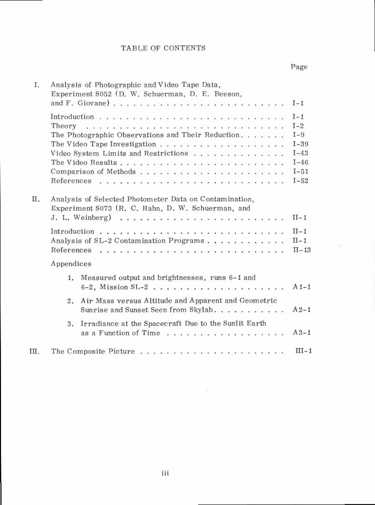
TABLE OF CONTENTS

Page

I. Analysis of Photographic and Video Tape Data,Experiment S052 (D. W. Schuerman, D. E. Beeson,and F. Giovane) 1-1

Introduction 1-1Theory 1-2The Photographic Observations and Their Reduction 1-9The Video Tape Investigation 1-39Video System Limits and Restrictions 1-43The Video Results 1-46Comparison of Methods 1-51References 1-52

n. Analysis of Selected Photometer Data on Contamination,Experiment S073 (R. C. Hahn, D. W. Schuerman, andJ. L. Weinberg) II-1

Introduction II-1Analysis of SL-2 Contamination Programs II-1References 11-13

Appendices

1. Measured output and brightnesses, runs 6-1 and6-2, Mission SL-2 A 1-1

2. Air Mass versus Altitude and Apparent and GeometricSunrise and Sunset Seen from Skylab A2-1

3. Irradiance at the Spacecraft Due to the Sunlit Earthas a Function of Time A3-1

IH. The Composite Picture ni-1

in

I. Analysis of Photographic and Video Tape Data, Experiment S052

Introduction

The S052 white light coronagraph on Skylab produced over 35,000

photographs of the solar corona. Approximately 10$ of these frames

contain evidence of particulates in the environs of the spacecraft.

The monitoring of this contamination was one of the prime objectives

of another coronagraph experiment, T025, (Henize and Weinberg, 1973)

but because the solar-side airlock was rendered useless throughout

the mission, that T025 objective could not be performed. Therefore,

the S052 "contaminated" frames constitute a unique body of data

which represents most, if not all, of the existing observations of

spacecraft-induced particulates. Since particulates of this sort can

be the limiting factor for optical and infrared experiments, it is

important to ascertain what information can be inferred about them

from the S052 photographs. As a preliminary to a larger, statistical

study, this investigation attempts (l) to define the S052 limits of

particle detectability, (2) to enumerate which particulate parameters

can be inferred, and (3) to note the accuracy with which these

parameters can be found in practice. The techniques used here are

those developed by us for the anticipated reduction of T025 data.

The actual film used in this pilot study is a first generation

copy of eleven sequential S052 frames containing particle tracks.

This film, along with pertinent instrumental data, has been provided

by R. MacQueen, the Principal Investigator of the S052 Experiment.

This photographic sequence, initiated on day of year (DOY) 159 at

0200 GMT, was selected only on the basis that it is representative

of the contamination data.

Theory

A nearby particle moving within the field of view of the S052

white light coronagraph registers as a track of width, a, and length,

1, on the film. The width of the track is defined by the circle-of-

confusion (here assumed uniform) resulting from an out-of-focus point

source and is a measure of the particle's distance, L, from the in-

strument. Since the coronagraph is focused at infinity, a and L are

related by

Af for a£e (l)a -

where A is the diameter of the objective, f is the focal length, and

e is the resolution of the system. When L is less than about 200

meters, a is larger than e and the particle's distance can be obtained

directly from the film. The two other space coordinates of the parti-

cle (X,Y) can be found from the particle's film coordinates (x,y):

X _ x and Y _ y_ (2)L ~ f L =: f .

The space velocity of the particle can only be obtained (except

for sign) if the track under consideration is entirely contained

within a single photograph. Consider any two points on the track

separated by a distance on the film of Al. It can be shown that the

time required for the particle image to traverse Al is related to

the frame exposure time, T, by

provided AL « JlWf YM2 (3)

1-2

The inequality always holds except for those few particles whose

motion is mostly along the line of sight. Therefore, the transverse

and radial space velocities are found by

AL and (4X)2 + MY)2'' '

The transverse space velocity, in turn, is related to the rate of

image motion across the film by

Ut (5)

It is this image motion which determines an effective particle expo-

sure time, T. At the center of the track, an elemental area of the

film is exposed to the moving circle-of-confusion of diameter a for

a time

a a L (6)= v " f vt " vt •

The film density of the particle track thus depends on T, while the

film background depends on the frame exposure time T.

Further photometric considerations of the particle track can be

used to infer the actual size of the particle. The energy/area

incident on the film in the center of a track can be calculated if

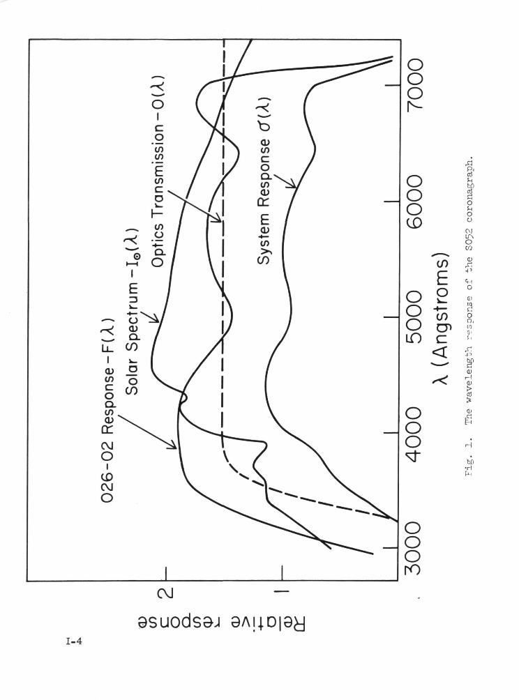
the spectral sensitivity of the system is known. The wavelength

response of the S052 coronagraph is shown in Figure 1. The mono-

chromatic energy response of the film due to an out-of-focus particle

image is then given by

1-3

I2ouoi

o

c. ,O

0'aoo.

-P

9

I

fi

to•H

1-4

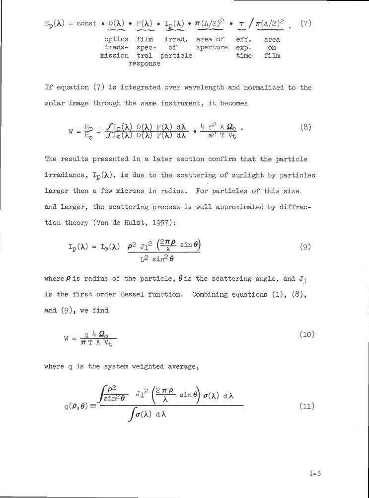
E ( X ) = const » ( X ) » F(X) • I ( X ) • nA/2} 2 • r TKa/2 2 t (?)Jpv __ _,_

optics film irrad. area of eff. areatrans- spec- of aperture exp. onmission tral particle time film

response

If equation (7) is integrated over wavelength and normalized to the

solar image through the same instrument, it becomes

Sp y~Ip(X) 0(X) F(X) dX It- f 2 A QQ . (8): =: 0(X) F(X) dX a2 T Vt

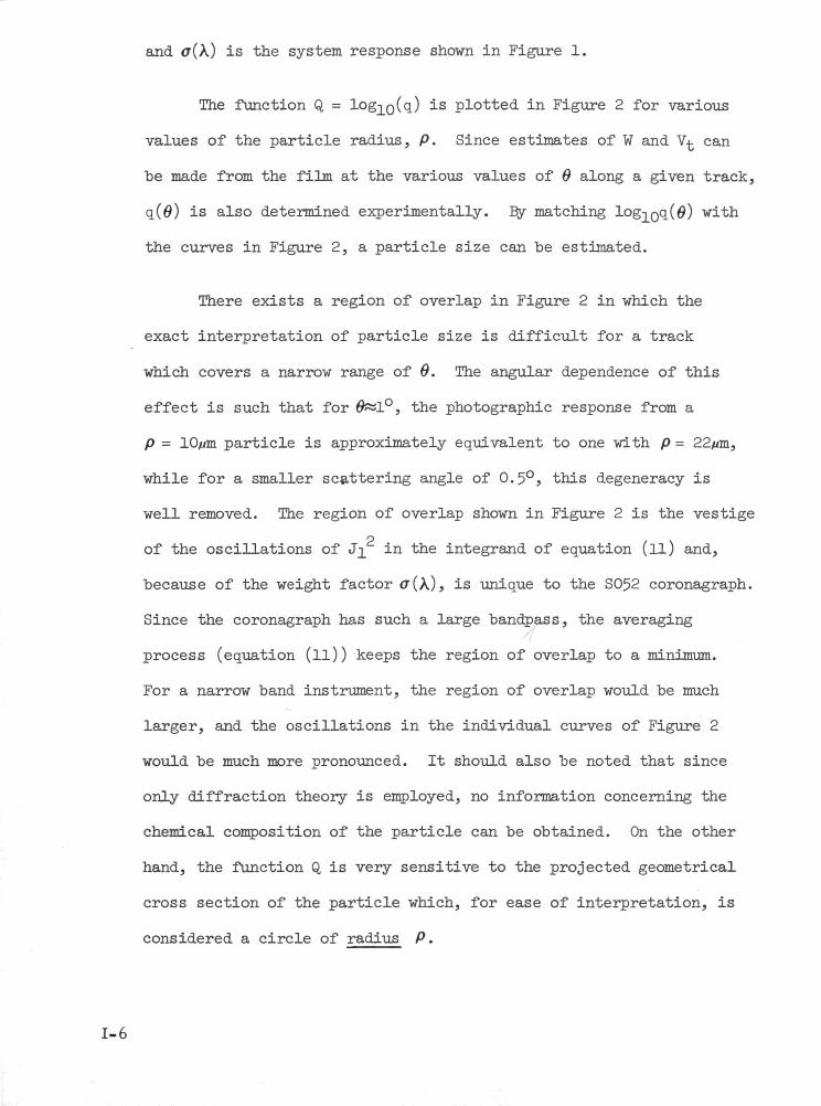
The results presented in a later section confirm that the particle

irradiance, Ip(X), is due to the scattering of sunlight by particles

larger than a few microns in radius. For particles of this size

and larger, the scattering process is well approximated by diffrac-

tion theory (Van de Hulst, 1957):

Ip(X) = I0(X) p2 j sin (9)

L2

where Pis radius of the particle, 0is the scattering angle, and Jj_

is the first order Bessel function. Combining equations (l), (8),

and (9), we find

= q Q (10)7TT A Vt

where q is the system weighted average,

dX(11)

1-5

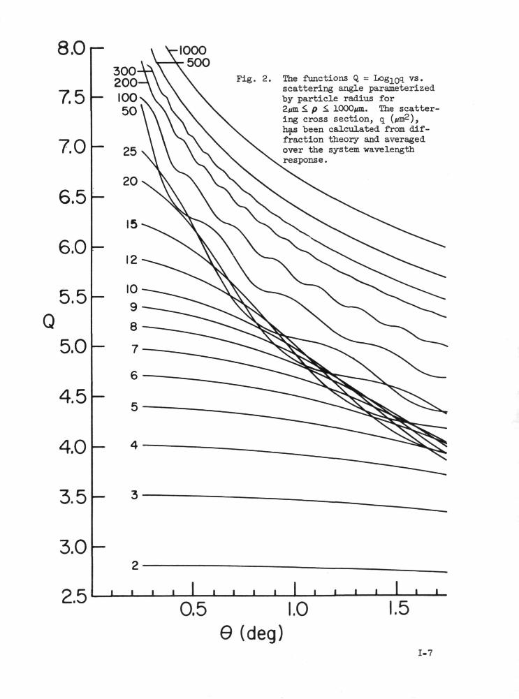
and a(X) is the system response shown in Figure 1.

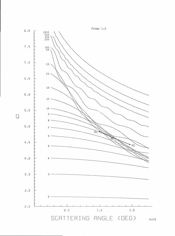
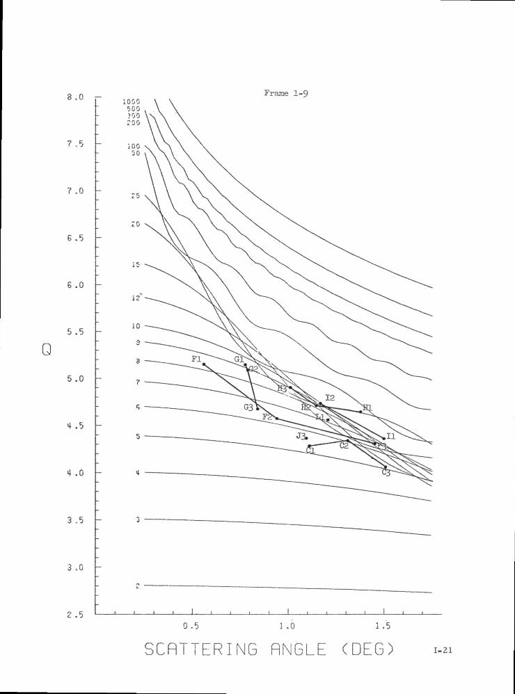
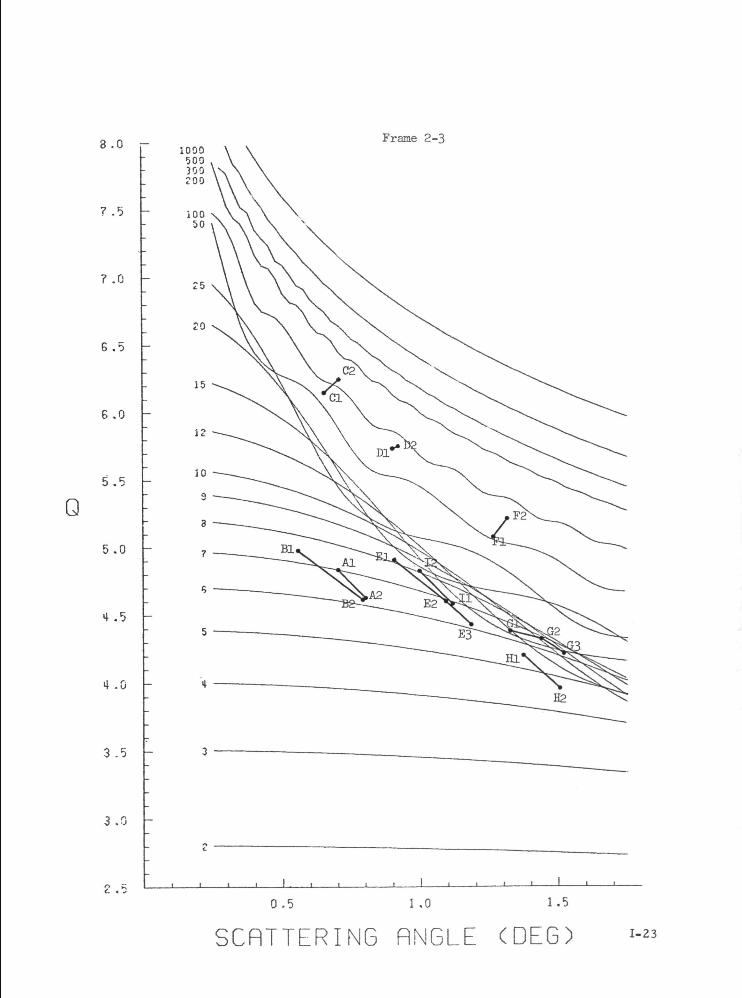
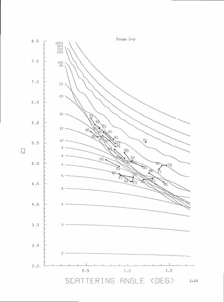
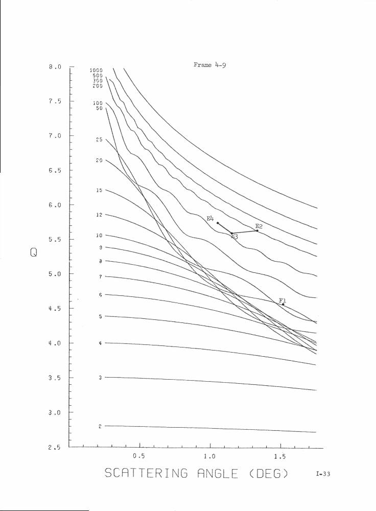
The function Q = log-j_Q(q) is plotted in Figure 2 for various

values of the particle radius, P. Since estimates of W and Vj. can

be made from the film at the various values of 0 along a given track,

q(0) is also determined experimentally. By matching log Qq( ) with

the curves in Figure 2, a particle size can be estimated.

There exists a region of overlap in Figure 2 in which the

exact interpretation of particle size is difficult for a track

which covers a narrow range of 0. The angular dependence of this

effect is such that for 0«1°, the photographic response from a

p = lOfim particle is approximately equivalent to one with p = 220m,

while for a smaller scattering angle of 0.5°, this degeneracy is

well removed. The region of overlap shown in Figure 2 is the vestigep

of the oscillations of Jj_ in the integrand of equation (ll) and,

because of the weight factor <r(A), is unique to the S052 coronagraph.

Since the coronagraph has such a large bandpass, the averaging

process (equation (ll)) keeps the region of overlap to a minimum.

For a narrow band instrument, the region of overlap would be much

larger, and the oscillations in the individual curves of Figure 2

would be much more pronounced. It should also be noted that since

only diffraction theory is employed, no information concerning the

chemical composition of the particle can be obtained. On the other

hand, the function Q is very sensitive to the projected geometrical

cross section of the particle which, for ease of interpretation, is

considered a circle of radius P.

1-6

8.0

7.5

7.0

6.5

6.0

5.5Q

5.0

4.5

4.0

3.5

3.0

2.5

vs.

0.5 1.09(deg)

1.5

1-7

When applying the above theory with the S052 coronagraph, the

plate scale is U82 + 3 arc-sec mm so that the focal length, f, of

the system is ^28 mm. The diameter of the aperture, A, is 31.23 mm.

A more complete description of the system is presented by MacQueen,

et al. (1971*).

1-8

The Photographic Observations and Their Reduction

The observations considered here are a sequence of pictures

taken in the "continuous patrol" mode of the S052 experiment. This

manually terminated mode consists of consecutive cycles of 82.5 s

duration. In each cycle, 3 frames are exposed for 9> 27, and 3 s

respectively. The time elapsed between the end of the 9 s exposure

and the start of the 2? s exposure is 18.5 s. Between the 2? s and

3 s exposures, the elapsed time is 0.5 s. The sequence of eleven

photos starts with a 3 s frame and ends with one of 27 s so that

there are four 3 s frames, four 9 s frames and three 27 s frames.

It was found that no tracks both started and stopped on the 27 s

exposure. They were not considered further, since the .locations of

the track end-points are crucial to size and velocity determinations.

From the eight remaining photographs, approximately 60 tracks were

selected for study.

The coordinates of the two end-points of each track, along with

the coordinates of a set of reference points on the film, were

measured on a Mann measuring engine. The frames were then positioned

in a S-3000 Specscan digital scanning densitometer, and the coor-

dinates were reset so as to correspond with the system established

when using the Mann engine. The Specscan was used to scan across

the track at up to five different places. The scans were all made

with a square aperture 12//m on a side. The choice of scan direction

(x or y) for each track was made by choosing that axis on which the

track had its shortest projection. Scans were also made of the cal-

ibration wedges in the center of each frame. All positional and

1-9

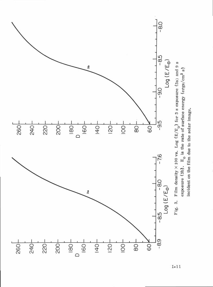
photometric data were stored on magnetic tape. A computer plot of

each scan then provided a convenient format from which to infer the

track width and the film densities of both the background and the

track center. Also, D-Log E curves were obtained for both the 3 s and

9 s exposures by using the calibration established by Poland, et al.

(1976). These curves are shown in Figure 3-

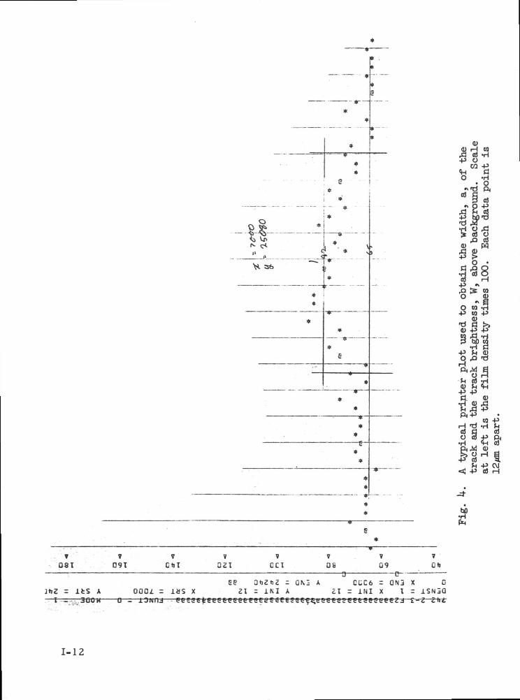
Figure k shows a typical working plot for extracting width and

brightness. A background density and a density near the center of

the track are first estimated by fitting horizontal lines at the ap-

propriate positions. The density scale is at the left of the print-

out, along with other particle and frame identification data. The

two densities are then converted to surface energies via the D-Log E

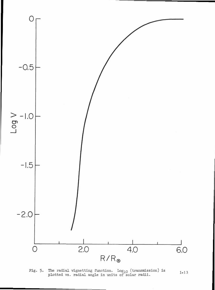
curves. We must take into account at this point that the system has

a severe, radial vignetting function whose purpose is to subdue the

inner corona so as to increase the effective dynamic range of the

system. This radial vignetting function is shown in Figure 5. After

correcting the background and mid-track energies for vignetting, they

are subtracted so that the resulting difference is the mid-track

particle energy, W, used in equations (8) and (10). The track width

is established by estimating the two points of the onset of the

density increase. Because each data point is separated by 12 m, the

width of the "bump" is determined. This width must be corrected for

the fact that the scan is not necessarily perpendicular to the length

of the track. When this rotation factor, which is obtained from the

coordinates of the end-points of the track, is applied to this esti-

mate, the width of the track, a, is obtained. With a and W known on

1-10

1OCDCM

aC\J

8'a '

OOvJ

OO

O00

QODi

U")

OCD

inCT)i

ccLU _' > 73 COLU g „„ ™ gcn -£ «Q co >

0)

8 §(D <U

« s

— W

« -S5 -2

bo *•"9 W

eds

•^J

h

"oCO

0£4-1

£

OCD00

OOvJ00

_LOCO

_LOCD

ooo

J_OO

OvJ — — — —

OCD

(DN

i

QCO

iLd

OCD

mCOi

£

3T3

w i

X ^

£ «ECC 0)o> t-.T3 3

•— coO>9 w>

o

Q) •-

1-11

<uH0)O

W

*_.< •

, *.*

v .v j

^

-g« O

,0 03

0 •d ^ o•r Oj O

rQ & M

• 1O tiT-H-P w -p

0)•o « >,«U -P -P

•P M <Uo ^a T)

33•M cfl «H-P -P5«5

cfl d 03o 3 +> PM•H . SH c3

fn -P CVJ«aj -P cfl H

fG 8 I C 9 T

1C U T

7CCI

7OS

J«?Z = its A OOOi - las X

7 709 OH

a c55 0«je«ie = QM A CCC6 = ON3 X 0

Zl = INI A Z\ - INI X t = ISN3QI --•- 30 —

1-12

0

-0.5

CPo

-1.5

-2.0

0 2.0 4.0R/R.

6.0

Fig. 5. The radial vignetting function. Log o (transmission) isplotted vs. radial angle in units of solar radii. 1-13

at least two portions of the track, and the length of the track known

as well, the theory of section II applies, and the following quanti-

ties can be determined from a single track:

(l) particle size - p

(2) transverse space velocity - V-t =\VX + Vy2 (without sign)

(3) azimuthal angle of transverse velocity - tan~ (Vy/Vx)

radial space velocity - Vr (without sign)

(5) characteristic distance of particle from spacecraft duringexposure . - L

An indication of the random uncertainties in the above determin

ations can be found in most cases because any particular quantity

has been over determined. For example, scans of the track at two

points are sufficient to determine Vt and Vr. In fact, if the width

of the track does not noticeably change along its length, then only

one scan is needed to determine Vt, and Vr is assumed to be zero.

In most cases, three scans of any track are used to determine V^.

Once Vt is established, the same three scans are used to determine

three values of W so that a triplet of points is located on the

scattering diagram of Figure 2. The extent to which this triplet

lies along a curve of constant p is indicative of the uncertainty in

particle radius. The measurements from any one track thus yield two

or three values of Vt and p. The spread in these numbers, when

seen in the context of a large number of particle tracks, indicates

the precision in which p and Vt can be determined. The same method

is used for determining the uncertainty in Vr and L.

The p, Vt plane makes a convenient format for the discussion

1-14

and presentation of the results for each track. Not only can p and

V.f. and their associated errors be plotted in this plane, but the limit

of particle detectability can also be represented by this scheme.

This is because q (p, 0) is proportional to WTV . as shown i» equation

(10). At a fixed value of 9, the quantity WT has a minimum value,

(WT)mj_n, below which no track can be distinguished. This minimum

value is influenced by the vignetting function shown in Figure 5>

and therefore depends upon radial position in the focal plane. How-

ever, (WT)m n is rather insensitive to the exposure time T. This is

because W is the energy due to the track above background. Since the

background increases with exposure time, the actual value of W de-

creases with increasing T. The quantity (WT) , however, is found

to be about the same for both the 3 s and 9 s exposures -

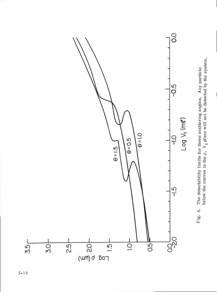
s' ^ settinS WT = Mmi in equation (10),V(0)

detectability limits can be established in the p, V^ plane for fixed

values of the scattering angle. These limits, parameterized by B,

are shown in Figure 6. We define the "system limit" to be the bottom

envelope of these curves.

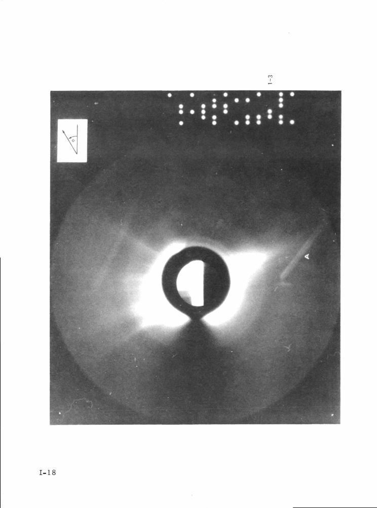
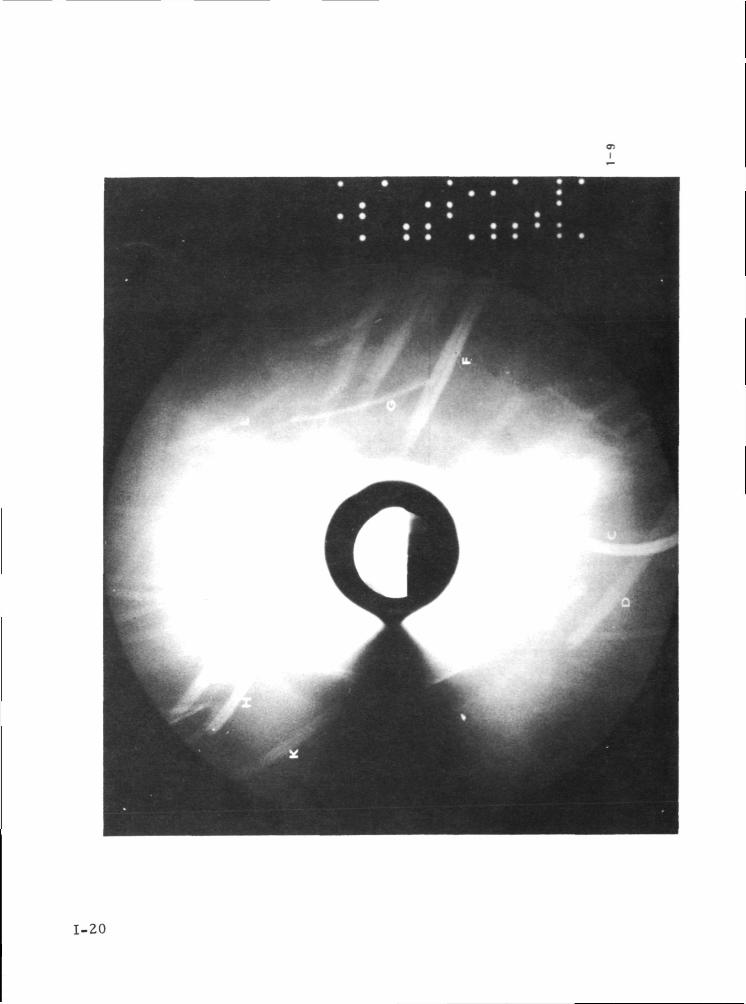
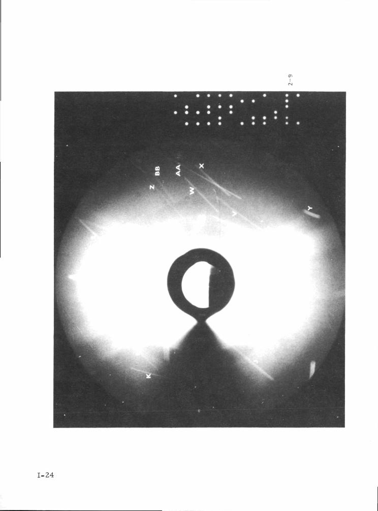
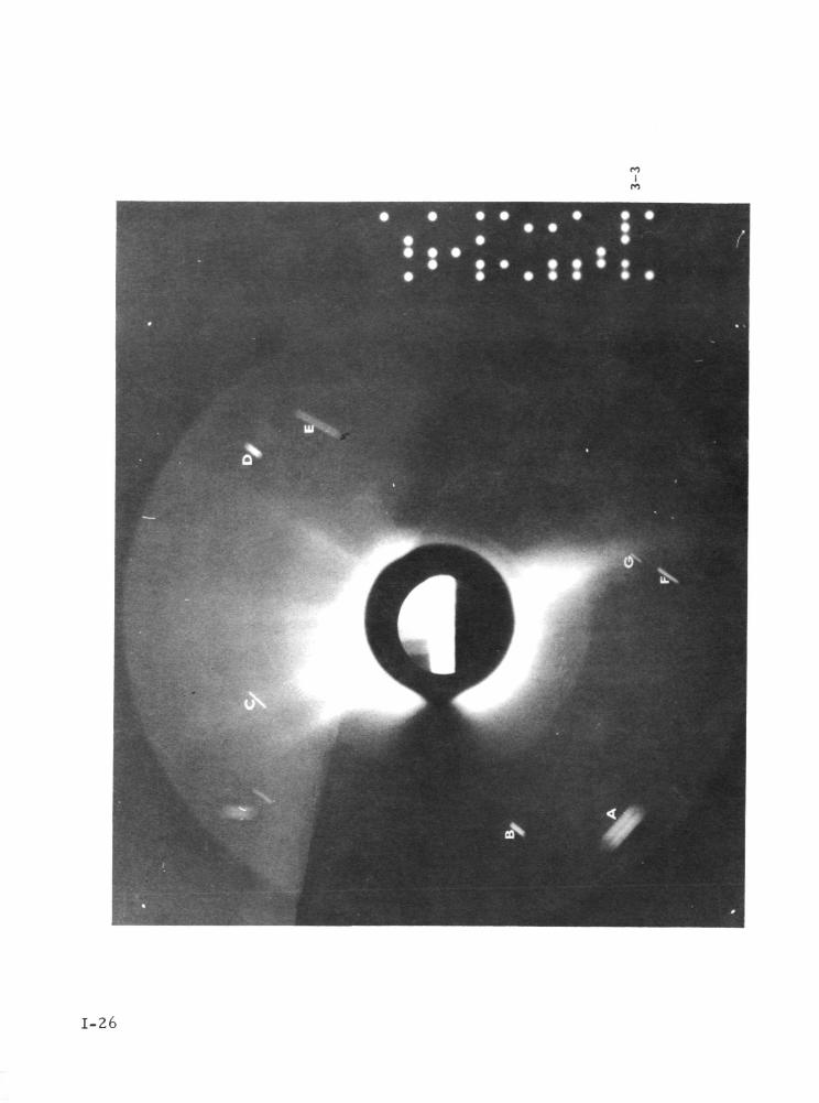
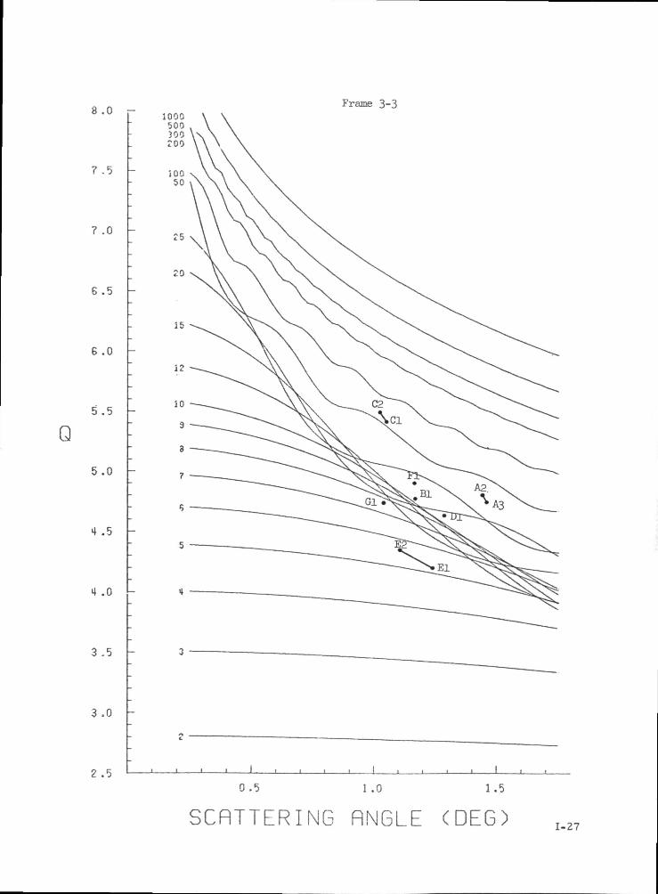
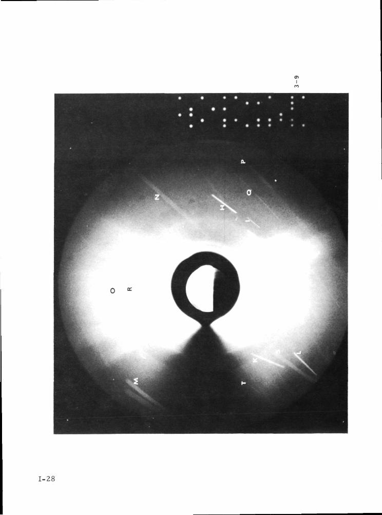
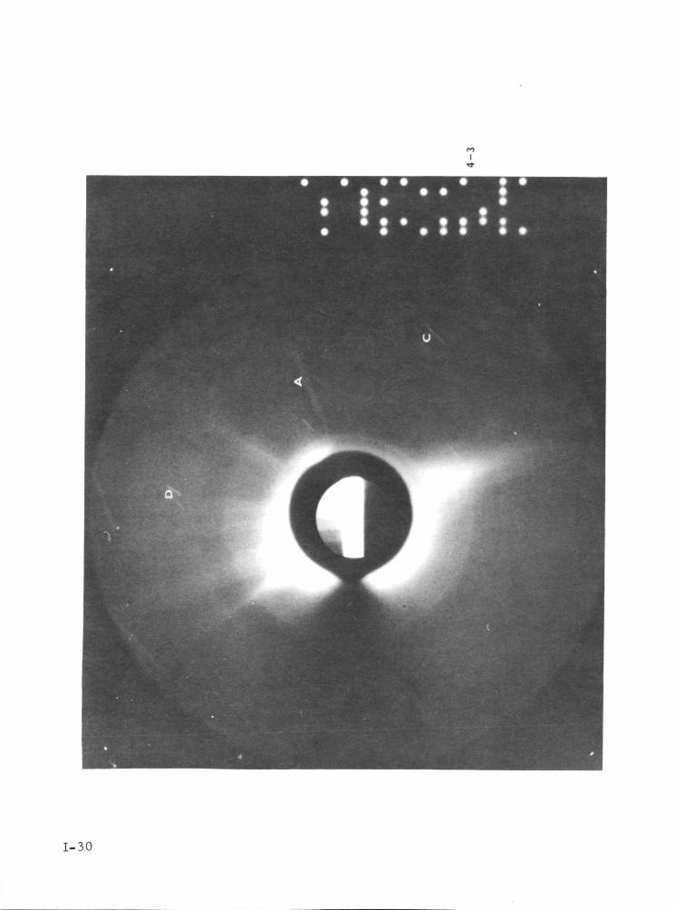
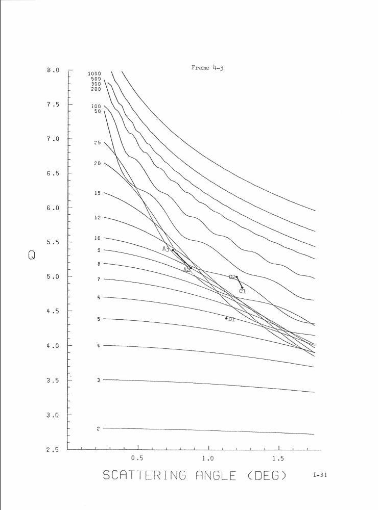
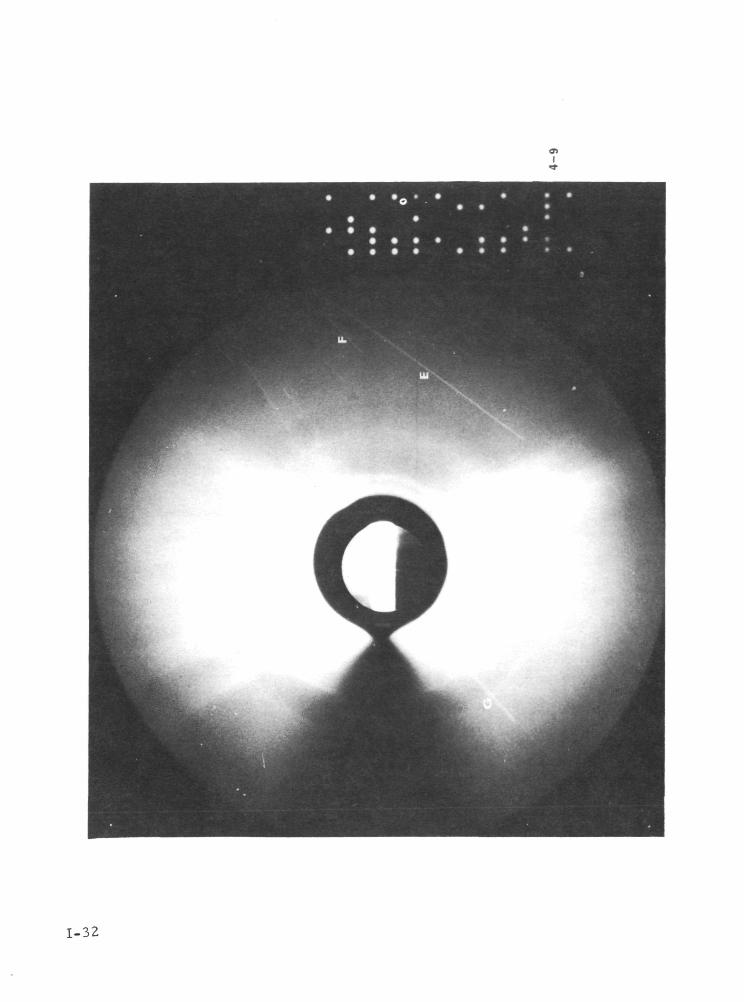
The eight photographs studied, along with the results, are shown

on the following pages. The photographs themselves are labelled by 2

numbers. The first digit, which ranges from 1 to k, designates the time

order of the photographs, and the second digit refers to the exposure

time (3 or 9 sees). The tracks considered are identified on the photo-

graph by letters. Each photo is accompanied on its reverse side by the scat-

tering diagram from which the particle sizes for each track have been

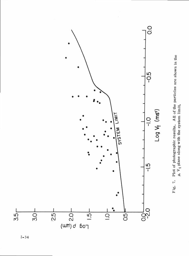
found. These are followed by a si.Tmtna.ry plot (Figure 7) of all points in

1-15

-r en

0)o

OT

01

<D

" oCrtbe -4-«

*~^ s °

<»

•S i

3 I

— I >• ~* t•° 3^S oo <u

I

(oiTl)d 6cn

1-16

This page intentionally blank

1-17

1-18

Q

8.0 r-

7 .5

7 .0

6.5

6 .0

5 .5

5 .0

4 .5

4 .0

3.5

Frame 1-3

3 ,0

2 .50,5 1.0 1.5

SCflTTERING flNGLE (DEG)

trI

1-20

8 .0 p- Frame 1-9

Q

7 .0

6 .5

6 .0

5 .5

5.0

4 .5

4 .0

3 .5

3,0

2.5 1 I I

0.5 1.0 1.5

SCflTTERING flNGLE (DEG)

1-22

Q

3.0 r

? .5

7 .0

6 .5

8 .0

5.5

5 .0

4.5

Frame 2-3

3.5

3.0

2 .5 I I L I i i I L-

0.5 1.0 1.5

SCflTTERING flNGLE (DEG) '-»

9

1-24

Q

8.0 r

7 .5

7 .0

6 .5

6 .0

5 .5

5 .0

.5

4 .0

3.5

Frame 2-9

3 .0

2 .0.5 1.0 1.5

SCflTTERING RNGLE (DEG) 1-25

fl

1-26

Q

8 .0 r-

7 .5

7 .0

6 .5

6 .0

5 .5

5 .0

4 .5

4 .0

3.5

Frame 3-3

3,0

2 .50 .5 1 .0 1 .5

SCflTTERING RNGLE CDEG) 1-27

lr*>

1-28

3 .0 i-

7-5 h

Q

6 .5

6 .0

5 .5

5 .0

4.5

4 .0

3.5

3 ,0

2 .5

Frame 3-9

_j I I I ! | i_

0.5 1.0 1.5

SCflTTERING flNGLE (DEG) 1-29

1-30

Q

8.0 r-

7 .5

? .0

6 .5

6 .0

5 .5

5 .0

.5

4 .0

3 ,5

3 ,0 h

Frame k-3

2 .50.5 1.0 1.5

SCflTTERING RNGLE (DEG)

1-32

.0 r

Q

7.5

7 .0

6 .5

6 .0

5 .5

5.0

.5

4 .0

3 .5

3 .0 h

2.50.5 1.0 1.5

SCnTTERING flNGLE (DEG) 1-33

inro

Oro oJ

QOJ

lO

o6

IT)O

Q 3

in.r

>0>o

0)X!

ICO

0)aoaha

S "->'5 fl•sl=5 S

CO

a »"3 2S ^^ 5u 'cs ^a bort C

fe^

.SP

1-34

the log p, log V-fc plane along with the system limit. It is evident

that the bottom of the distribution of points is interrupted by the

system limit. The distribution itself undoubtedly continues downward

to include particles smaller than the system can detect. On the

other hand, if particles larger than 100/ym truly are present, they

should be observable. Because of this, we interpret the upper cutoff

of particle sizes to be a real effect and representative of the space-

craft environment at the time the pictures were taken. The upper

bound on Vt, on the other hand, arises because of the restriction

that a particle image must both start and stop on the frame. It

does not represent the true velocity limit of the contamination cloud.

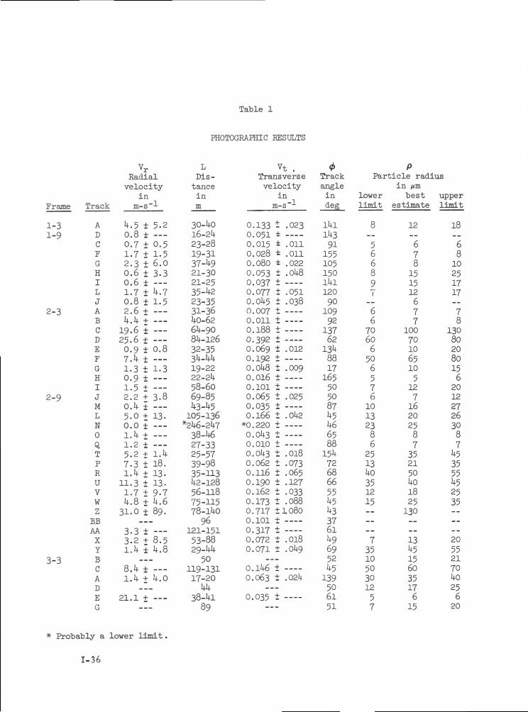
A summary of all the inferred parameters is presented in Table

1. In some cases, either a densitometer scan was positioned incor-

rectly on the track, or the track was not distinguishable above the

background so that some of the parameters could not be determined.

These cases are represented by dashes in the appropriate columns of

Table 1. In that table, the frames are presented in chronological

order along with the track designation. The average radial velocity

of each particle is presented in the next column along with its

standard deviation if two or more determinations of Vr were made.

The next column contains the range of particle distances as determined

from measurements of the track width. The next two columns specify

the transverse velocity. The column marked Vt gives the magnitude

and its standard deviation (where possible) and the column labelled

<f> gives the track direction as seen on the photograph. The definition

of 0 is provided by the inset in the photograph 1-3- Since there is

1-35

Table

PHOTOGRAPHIC RESULTS

Frame

1-31-9

2-3

2-9

3-3

Track

ADCFGHILJABCDEFGHIJMLN0QTPRUVWzBBAAXYBCADEG

vrRadialvelocity

inm-s~l

U.5 ± 5-20.8 ±0.7 + 0.51.7 + 1-52.3 + 6.00.6 ± 3-30.6 ± —1.7 ± U.70.8 ± 1.52.6 + —U.U + —19.6 + —25.6 ± —0.9 + 0.87.U ± —1.3 ± 1.30.9 ± —1.5 + —2.2 + 3-8O.U ± —5.0 + 13.0.0 ± —l.U + —1.2 ± —5.2 + l.U7.3 + 18.l.U + 13.11.3 + 13-1.7 ± 9-7U.8 + U.631.0 + 89.

—3-3 + —3.2 + 8.5l.U ± U.8

—8.U ± --l.U + U.O

—21.1 ± — ----

LDis-tanceinm

30-UO16-2U23-2819-3137-U921-3021-2535-U223-3531-36UO-626U-908U-12632-353U-UU19-2222-2U58-6069-85U3-U5105-136*2U6-2U738 -U627-3325-5739-9835-113U2-12856-11875-11578-lUo96

121-15153-8829-UU50

119-13117-20UU

38-Ul89

* Probably a lower limit .

1-36

Transversevelocity

in

Particle radiusin //m

lower best upperlimit estimate limit

0.1330.0510.0150.0280.0800.0530.0370.077O.OU50.0070.0110.1880.3920.0690.192O.OU80.0160.1010.0650.0350.166

*0.220O.OU30.010O.OU30.0620.1160.1900.1620.1730.7170.1010.3170.0720.071

t .023±± .011± .011± .022t .OU8+± .051+ .038++++± .012++ .009++

± .025+1 .OU2++++ .018± .073+ .065± .127± .033+ .088+ 1080+++ .018± .OU9

0.1U6 ±0.063 ± .02U

0.035 ±

8

56689

6670606506576101323862513ko351215

7351050301257

12

678151512677

10070106510512716202587352150ko1825130

13

15603517615

18

6810251717

78

130802080156201227263087

3555

2535

20552170UO25620

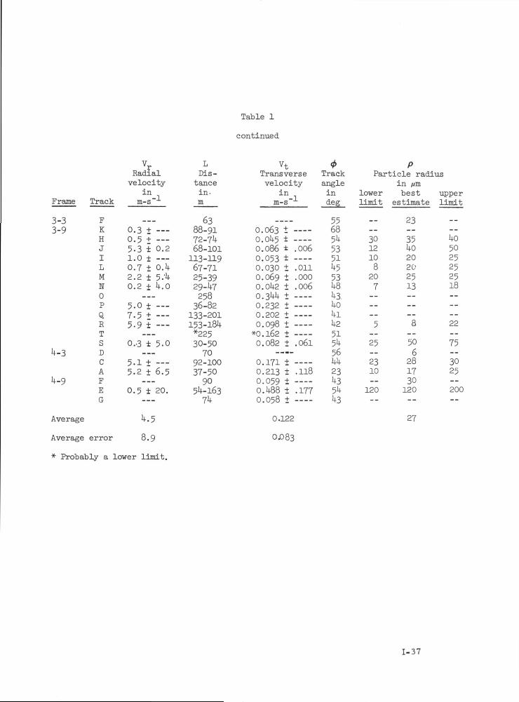
Table 1

continued

Frame

3-33-9

1+-3

1+-9

Average

Average

Track

FKHJILMII0PQRTSDCAFEG

error

Radialvelocity

inm-s

0.3 + —0.5 + —5-3 ± 0.21.0 ± - —0.7 ± 0.1+2.2 ± 5A0.2 + l+.O

5.0 +7.5 + —5.9 + —___

0.-3 ± 5-0

—5-1 ± —5.2 ± 6.5

—0.5 ± 20.

M

8.9

LDis-

tancein.m

6388-9172-7*+68-101

113-11967-7125-3929-1+7258

36-82133-201153-181+*22530-50

7092-10037-50

905^-163

7l+

* Probably a lower l imit .

vt <t>Transverse Trackvelocity angle

in inm-s deg

0.063 ±O.Ql+5 ±0.086 ±0.053 ±0.030 ±0.069 ±O.Ql+2 +0.31+1+ +0.232 +0.202 t0.098 ±K).l62 +0.082 +

- —0.171 +0.213 ±0.059 ±0.1+88 ±0.058 +

0.122

OJ083

.006

.011

.000

.006

.061

.118

.177

5568514.53511+553U8U3UOin1+2515)456Mt23li"3ch||O

Particle radiusin tim

lower best upperlimit estimate limit

3012108207

5

25

2310

120

23

35ho20202513

8

506281730120

27

5025252518

22

75

3025

200

1-37

no way to tell the sign of the direction of the particle, the range

of angle is limited to 0<*<l80.

The last 3 columns provide the best estimate of upper and lower

bounds to the particle size. These are inferred from the scattering

diagrams presented with each photo. The average particle size as

determined from the best estimate column is 27/ m. Since the sample

is biased at least by the system limit, this number represents only

an upper limit on the average of the true distribution.

1-38

The Video Tape Investigation

A very convenient feature of the video tape provided to us is

that it has been modified so that the GMT, in one second intervals,

is displayed in the center of the frame. This provides a way of

labeling particles as well as measuring time intervals for velocity

estimates. The various segments of the tape are summarized in Table

2. Two of those segments were selected for analysis: days 166 and

220.

Day 166 is of the utmost importance due to the presence of

Saturn in the field of view. Because the video mode does not include

the step-wedge calibration image, Saturn offers the best available

means for a photometric calibration. Also, the plate scale for the

video mode is different for the x and y directions as is obvious

from the elliptical appearance of the occulting disk. Since the

instrument is rotated approximately 90° during the day l66 tape seg-

ment, a continuous set of data is available to determine these two

scale factors by using Saturn's known elongation of 1.10°.

Day 220 was chosen to be analyzed because this segment offers a

wide variety of particle speeds and image sizes. The random direc-

tions of motion indicate that the particles are probably not associated

with a dump, and they might therefore be more representative of the

ambient environment.

The exposure time of the video system is 1/60 s, so that, at

any instant, most particle images are not tracks as on the photographs,

but rather well-defined circles-of-confusion. The diameter of the

1-39

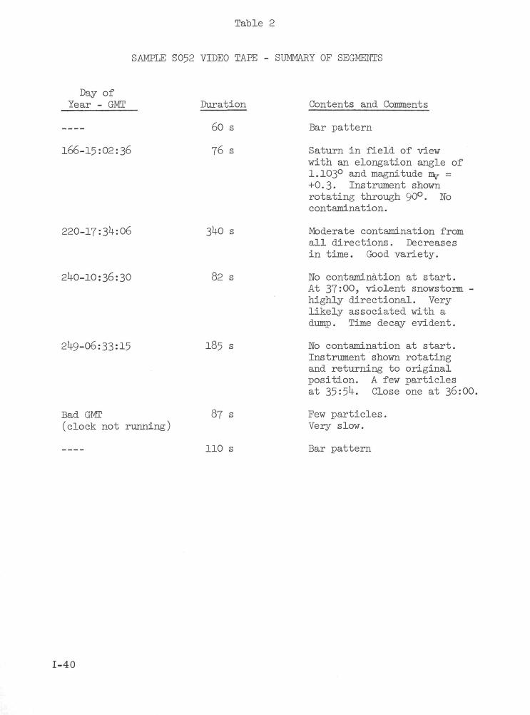
Table 2

SAMPLE S052 VIDEO TAEE - SUMMARY OF SEGMENTS

Day ofYear - GMT

166-15:02:36

220-17:3*1:06

2 0-10:36:30

2*4-9-06:33:15

Bad GMT(clock not running)

Duration

60 s

76 s

3^0 s

82 s

185 s

87 s

110 s

Contents and Comments

Bar pattern

Saturn in field of viewwith an elongation angle of1.103° and magnitude my =+0.3. Instrument shownrotating through 90°. Nocontamination.

Moderate contamination fromall directions. Decreasesin time. Good variety.

No contamination at start.At 37:00, violent snowstorm -highly directional. Verylikely associated with adump. Time decay evident.

No contamination at start.Instrument shown rotatingand returning to originalposition. A few particlesat 35:5*4-. Close one at 36:00.

Few particles.Very slow.

Bar pattern

1-40

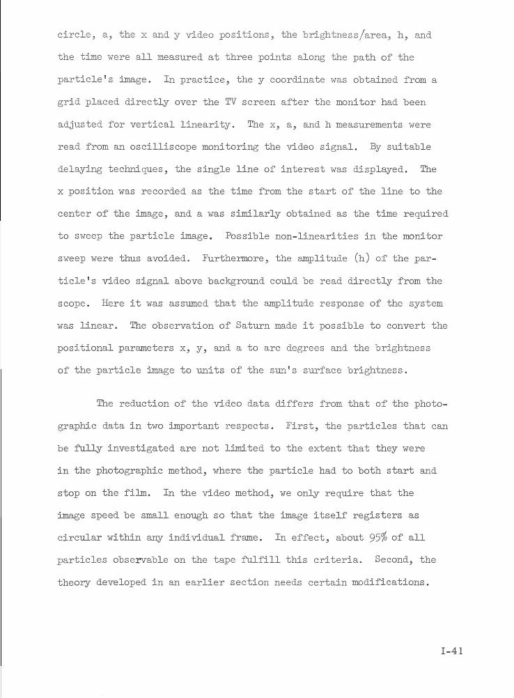
circle, a, the x and y video positions, the brightness/area, h, and

the time were all measured at three points along the path of the

particle's image. In practice, the y coordinate was obtained from a

grid placed directly over the TV screen after the monitor had been

adjusted for vertical linearity. The x, a, and h measurements were

read from an oscilliscope monitoring the video signal. By suitable

delaying techniques, the single line of interest was displayed. The

x position was recorded as the time from the start of the line to the

center of the image, and a was similarly obtained as the time required

to sweep the particle image. Possible non-linearities in the monitor

sweep were thus avoided. Furthermore, the amplitude (h) of the par-

ticle's video signal above background could be read directly from the

scope. Here it was assumed that the amplitude response of the system

was linear. The observation of Saturn made it possible to convert the

positional parameters x, y, and a to arc degrees and the brightness

of the particle image to units of the sun's surface brightness.

The reduction of the video data differs from that of the photo-

graphic data in two important respects. First, the particles that can

be fully investigated are not limited to the extent that they were

in the photographic method, where the particle had to both start and

stop on the film. In the video method, we only require that the

image speed be small enough so that the image itself registers as

circular within any individual frame. In effect, about 95$ of all

particles observable on the tape fulfill this criteria. Second, the

theory developed in an earlier section needs certain modifications.

1-41

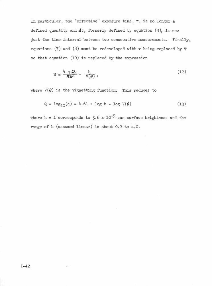
In particular, the "effective" exposure time, T, is no longer a

defined quantity and At, formerly defined by equation (3), is now

just the time interval between two consecutive measurements. Finally,

equations (?) and (8) must be redeveloped with T being replaced by T

so that equation (10) is replaced by the expression

**• ga h (12)~

where V(#) is the vignetting function. This reduces to

Q = Iog10(q) = >K 61 + log h - log V(0) (13)

f -Qwhere h = 1 corresponds to 3-o x 10 ' sun surface brightness and the

range of h (assumed linear) is about 0.2 to U.O.

1-42

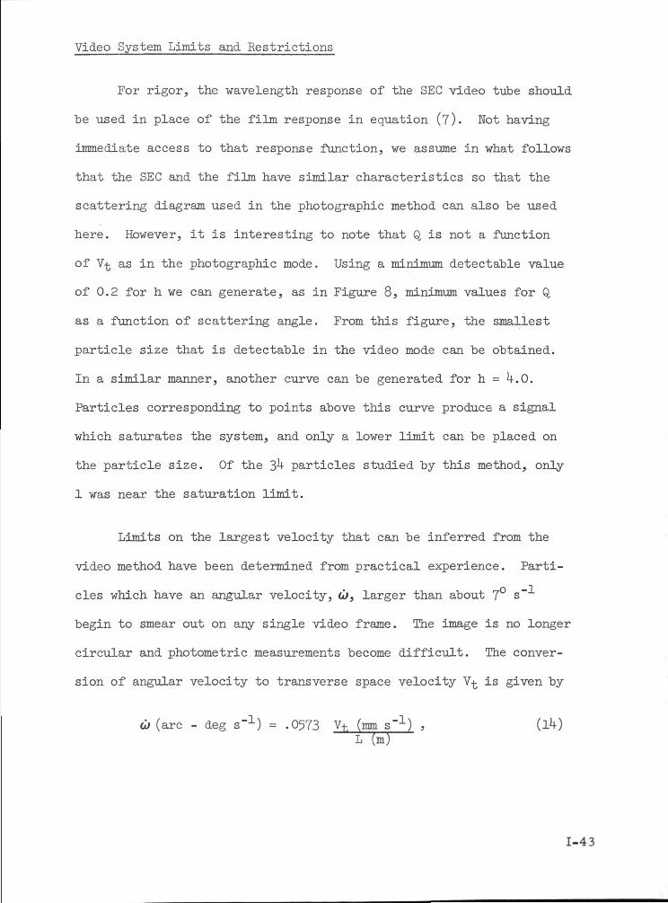
Video System Limits and Restrictions

For rigor, the wavelength response of the SEC video tube should

be used in place of the film response in equation (7). Not having

immediate access to that response function, we assume in what follows

that the SEC and the film have similar characteristics so that the

scattering diagram used in the photographic method can also be used

here. However, it is interesting to note that Q is not a function

of V-fc as in the photographic mode. Using a minimum detectable value

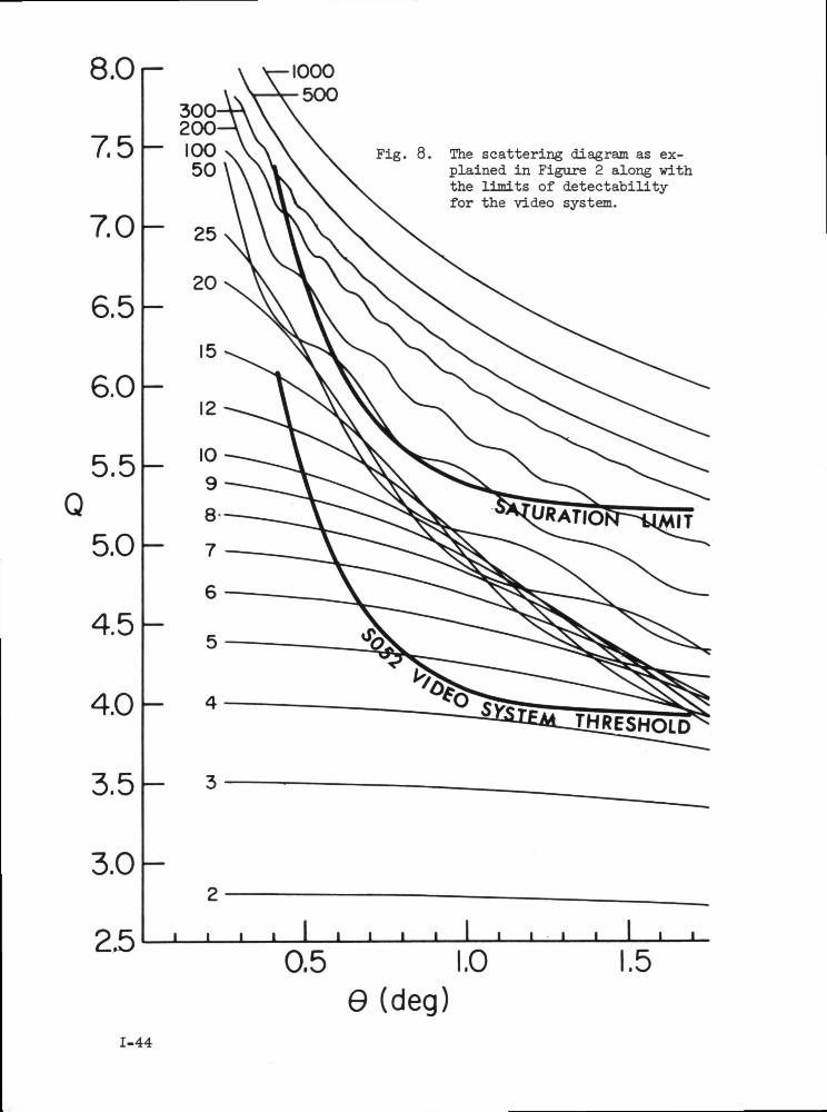
of 0.2 for h we can generate, as in Figure 8, minimum values for Q

as a function of scattering angle. From this figure, the smallest

particle size that is detectable in the video mode can be obtained.

In a similar manner, another curve can be generated for h = k.Q.

Particles corresponding to points above this curve produce a signal

which saturates the system, and only a lower limit can be placed on

the particle size. Of the 3^ particles studied by this method, only

1 was near the saturation limit.

Limits on the largest velocity that can be inferred from the

video method have been determined from practical experience. Parti-

cles which have an angular velocity, (j, larger than about 7° s

begin to smear out on any single video frame. The image is no longer

circular and photometric measurements become difficult. The conver-

sion of angular velocity to transverse space velocity V^ is given by

W (arc - deg s"1) = .0573 V-h (mm s"1) ,' L (m)

1-43

8.0

7.5

7.0

6.5

6.0

5.5Q5.0

4.5

4.0

3.5

\- 4

k- 3

Fig. 8. The scattering diagram as ex-plained in Figure 2 along withthe limits of detectabilityfor the video system.

3.0

250.5 1.0

0(deg).5

1-44

so that

(Vt)max in mm s"1 = 122 L(m) for L 75 m. (15)

The restriction on L here is much smaller that the 200 m used in the

photographic method, because the resolution of the video system is

less than half that of the film. Saturn's image has a diameter of

.025° + 00k. With this resolution limit, distances beyond 75 meters

or so from the spacecraft can not be determined accurately (see

equation (l)). The space velocities, from equations (2) and (),

also contain L. For L > 75 meters, the velocities so obtained repre-

sent only a lower limit. In the presentation of the results, such

lower limits will be noted by an asterisk.

1-45

The Video Results

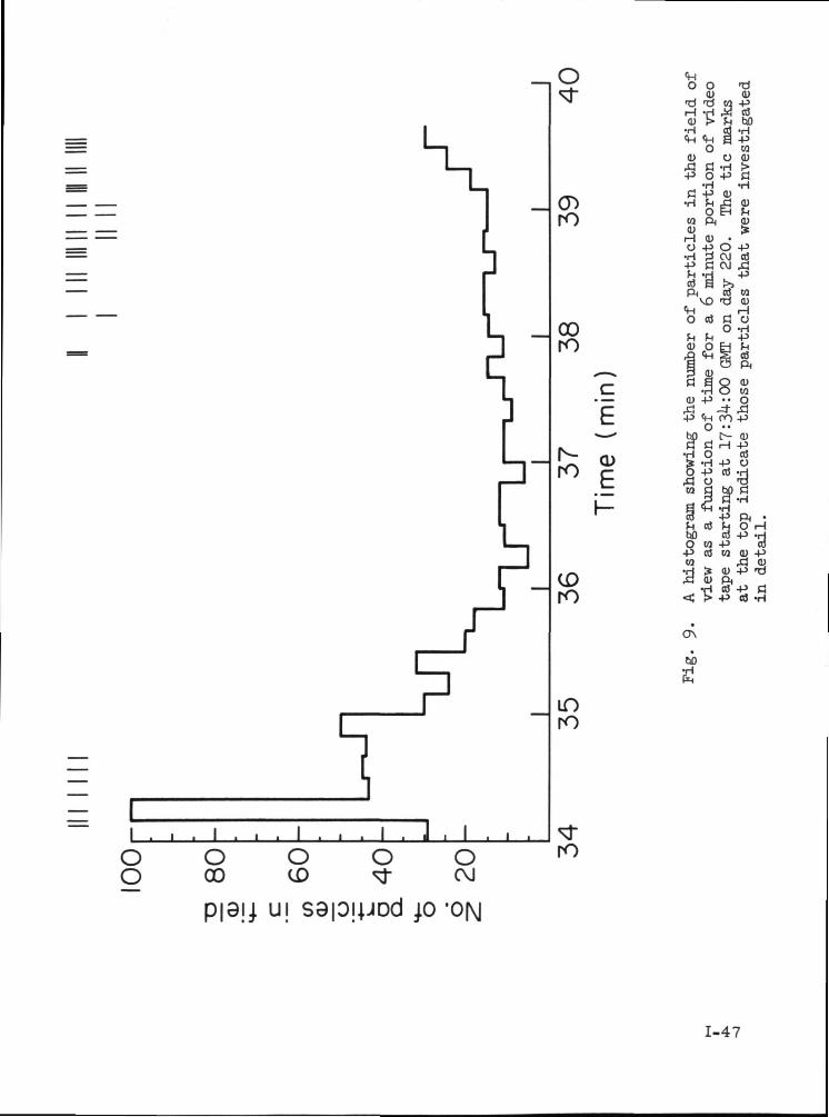
A sample of 3^ particles was selected for detailed investiga-

tion from a six minute portion of tape commencing at 17:3 *00 GMT on

DOY 220. Figure 9 is a histogram showing the number of particles in

the field of view as a function of time. From this total population,

3 4- particles were selected at the times indicated by the tic marks

in the top of the figure. The selection was made so as to include a

variety of particle speeds, brightnesses, and sizes. Any bias induced

by the selection procedure was unintentional.

At least three sets of measurements were made for each particle

so that some measure of uncertainty would be obtained; Table 3 shows

the results. The particles are listed chronologically as they appear

in Figure 9- Column 2 shows the angular speed of the particle through

the field of view. Two values of this quantity could be derived from

the positional and time data; the average of these two is shown, along

with the standard deviation.

The next two columns are closely related. The one designated

by L shows the range of particle distances as inferred by three

measurements of particle diameter, a. The entries that are starred

probably represent lower limits, since distances beyond 75 m cannot

be determined. The radial velocities are found from the L values

and the time intervals between their measurements. At least two

values for Vr were determined for each particle; their average and

standard deviation are shown. Those entries marked by an exclamation

point are not internally consistent in that the two values for Vr

1-46

=I I I

O

CT>rO

GOro

0>

E

CDro

inro

OO

O00

OCD

OCO

ro

O OQJ

-d -dH -H

«H <HO

0)^ a-P O

•Ha -p•H Vt

OW P)0)

H (1)O -P•rl 2-p Sfn -d03 3

•d0)

w -p,2 03fc hO3 -Ha -Pno 0

•H f>•P S

•H0)

s-p

CMCMCM 03

,3

«HO o3

(U Ofl "H

03 viT) Q)

c oO -H

+3hOj

a$0) -P

8 0)

-pO

on -PD- Q)H -P

03-P O

M o3bOO w

•P o3

•d I*fl 0)

•H4} Q| i

l°'dW <U -P

rcj ^)fl) -p 'dQiff-P CS

-P 03 -H

Ul 'Of\J

1-47

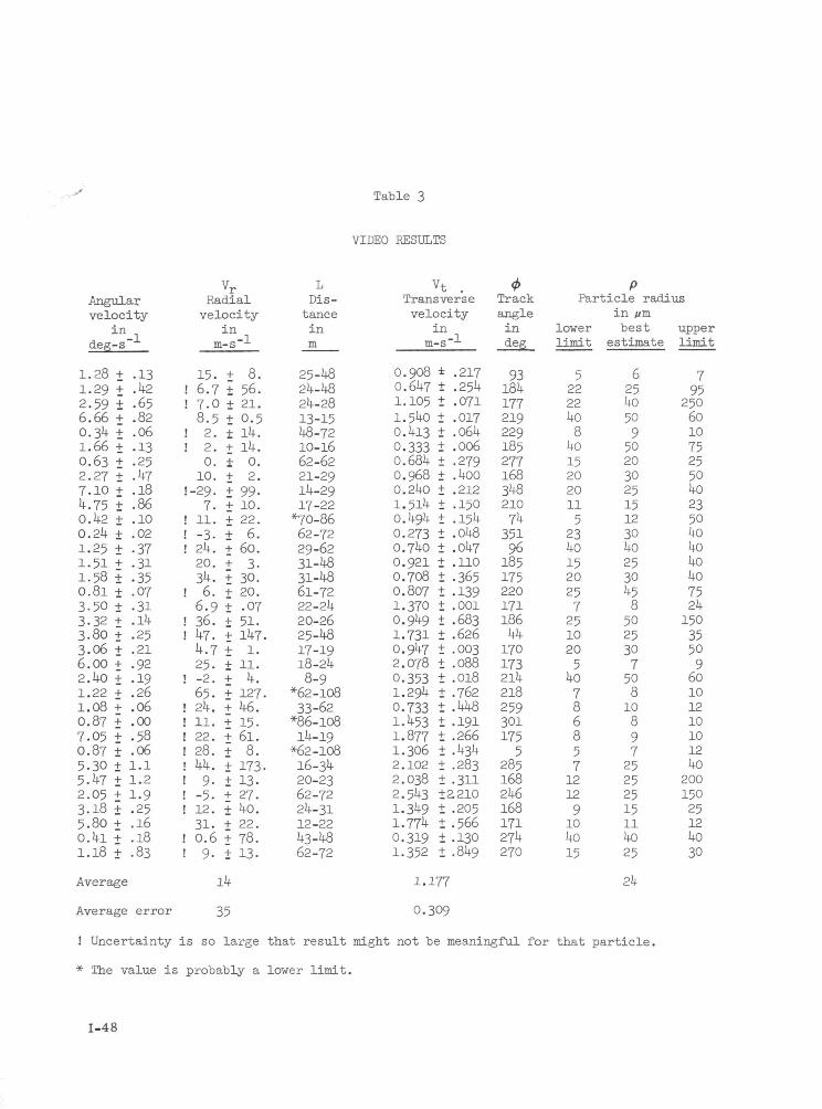
Table 3

VIDEO RESULTS

Angularvelocity

ln 1deg-s

1.281.292.596.660.341.660.632.277.104.750.420.241.251.511.580.813-503-323-803-066.002.401.221.080.877.050.875.305.472.053.185.800.4l1.18

++++++++++++++++++++++++++±+++++++

.13

.42

.65

.82

.06

.13

.25

.47

.18

.86

.10

.02• 37• 31.35.07.31.14.25.21.92.19.26.06.00.58.06l.l1.21-9.25.16.18.83

Average

Average error

Radialvelocity

in im-s

15.! 6.7! 7.08.5

! 2.! 2.

0.10.

!-29.7.

! 11.! -3.! 24.20.34.

! 6.6.9

! 36.! 47.4.725-

! -2.65-

! 24.! 11.! 22.! 28.! 44.! 9-! -5.! 12.31.

! 0.6I 9-

++++±++++++++++++±++±++++++++++++±

— _L

8.56.21.0.514.14.0.2.99.10.22.6.60.3.30.20..0751.147.1.11.4.127.46.15.6l.8.173.13-27.40.22.78.13.

LDis-tanceinm

25-4824-4824-2813-1548-7210-1662-6221-2914-2917-22*70-8662-7229-6231-4831-4861-7222-2420-2625-4817-1918-248-9

*62-!0833-62*86-!0814-19*62-!0816-3420-2362-7224-3112-2243-4862-72

14

35

vt .Transversevelocity

intn-s"-1-

0.908 ±0.647 ±1.105 ±1.540 +0.413 +0.333 ±0.684 ±0.968 ±0.240 ±1.514 ±0.494 ±0.273 ±0.740 +0.921 ±0.708 ±0.807 11.370 +0.949 ±1.731 ±0.947 ±2.078 t0.353 ±1.294 +0.733 ±1.453 ±1.877 +1.306 ±2.102 +2.038 +

.217

.254

.071

.017

.064

.006

.279

.400

.212

.150

.154

.048

.047

.110

.365

.139

.001

.683

.626

.003

.088

.018

.762

.448

.191

.266

.434

.283• 311

2.543 ±22101.349 ±1.774 +0.319 ±1.352 i

1.177

0.309

.205

.566

.130

.849

Trackanglein

93184177219229185277168348210743519618517522017118644170173214218259301175

5285168246168171274270

Particle radiusin ftm

lower best upperlimit estimate limit

5222240840152020115

234015202572510205

73685712129104o15

625405095020

25151230ko2530'45

85025307503103972525251511kG25

24

795

25060107525504o235040ko

ko752415035509601012101012ko2001502512ko30

! Uncertainty is so large that result might not be meaningful for that particle.

* The value is probably a lower limit.

1-48

have opposite signs or one value of Vr was zero. An entry so desig-

nated might not be meaningful for describing the motion of that single

particle. Nevertheless, the results are included because of their

importance in a statistical sense.

The average transverse velocities along with the standard dev-

iations are shown in the fifth column. These also depend on the L

measurements (see equations (2) and (U)), and those entries that are

starred may be lower limits. The direction of particle motion,

corrected for the unequal scale factor, is shown in the next column.

Consider a right-handed coordinate system superimposed over the TV

monitor screen with positive x to the right side as viewed. A 0

of 0° is along the x axis in the positive direction, and 0 of 90

is "up" on the screen. The uncertainty in this measurement is small--

less than a few degrees.

The last three columns represent best estimates and uncertain-

ties in particle radius. For each particle, at least three points

were placed on the scattering diagram and a "best estimate" was made.

Large and small limits were also established. It is interesting to

note that the average value of the best estimate column is 2 /ym.

This compares with the value of 27//m found from the photographic

method. There is no compelling reason to expect,a priori, that these

two size distributions should be similar, but the fact that they do

coincide gives one a certain amount of confidence in the correctness

of the two methods. This is particularly true since the photometric

calibration is entirely different for the two techniques. We also

1-49

find for the video data, as with the photographic, that the decrease in

particle number with increasing particle size is a real feature of the

distribution. The upper cut-off at about 50 m is assumed truly repre-

sentative of the contamination studied. Larger particles, if they

existed, would tend to saturate the video response, and saturation was

riever quite achieved.

1-50

Comparison of Methods

Essentially the same parameters concerning particle contamina-

tion can be obtained from either the photographic or video technique.

In terms of accuracy, the photographic method is characterized by an

error in V^. of the order of 80 mm s as opposed to 300 mm s~^ for

the video. Similarly, the photographic error in Vr is only 9 ni s" -

compared with 35 m s~-^ for the video. Also, the photographic method,

because of its higher resolution, can be used to fully investigate

particles out to 200 meters - more than twice the distance that can

be investigated with the video method. And finally, the photographic

method may be seen from Tables 1 and 3 to be somewhat more accurate

for estimating particle size.

On the other hand, only the video method can handle transverse

space velocities larger than a few hundred mm s~ -. In this method,

almost all of the observed particles can be analyzed, and thus selec-

tion effects are far less severe than for the photographic method

where only the low velocity tail of the distribution can be studied.

The other great advantage of the video method is the ease of data

taking. The raw data can be read from a monitor grid and oscilliscope

with very little effort compared to the time consuming techniques of

densitometer tracing and film position measuring. For these two

major reasons, the video method is highly recommended as the best

one to use for analyzing the large populations of individual particles

necessary to statistically characterize the contamination about Skylab.

1-51

References

Henize, K. G. and J. L. Weinberg, Astronomy Through the SkylabScientific Airlocks, Sky and Telescope, 5, 272-276, 1973.

MacQueen, R. M. , J. T. Gosling, E. Hildner, R. H. Munro, A. I. Poland,and C. L. Ross, Proceedings of the Society of Photo-OpticalInstrumentation Engineers 7 kh, 207,

Poland, A. I., J. T. Gosling, R. M. MacQueen, and R. H. Munro, TheRadiance Calibration of the High Altitude Observatory White LightCoronagraph on Skylab, submitted to Applied Optics, 1976.

Van de Hulst, H. C., Light Scattering by Small Particles, John Wileyand Sons, Inc., New York, pp. 103-110, 1957-

1-52

II. Analysis of Selected Photometer Data on Contamination, Experiment S073

Introduction

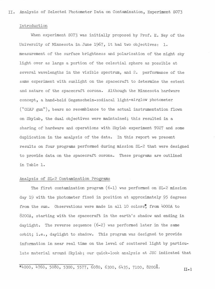
When experiment S073 was initially proposed by Prof. E. Ney of the

University of Minnesota in.June 196?> it had two objectives: 1.

measurement of the surface brightness and polarization of the night sky

light over as large a portion of the celestial sphere as possible at

several wavelengths in the visible spectrum, and 2. performance of the

same experiment with sunlight on the spacecraft to determine the extent

and nature of the spacecraft corona. Although the Minnesota hardware

concept, a hand-held Gegenschein-zodiacal light-airglow photometer

("GZAP gun"), bears no resemblance to the actual instrumentation flown

on Skylab, the dual objectives were maintained; this resulted in a

sharing of hardware and operations with Skylab experiment T027 and some

duplication in the analysis of the data. In this report we present

results on four programs performed during mission SL-2 that were designed

to provide data on the spacecraft corona. These programs are outlined

in Table 1.

Analysis of SL-2 Contamination Programs

The first contamination program (6-1) was performed on SL-2 mission

day 19 with the photometer fixed in position at approximately 95 degrees

from the sun. Observations were made in all 10 colors* from hOOOA to

8200A, starting with the spacecraft in the earth's shadow and ending in

daylight. The reverse sequence (6-2) was performed later in the same

orbit; i.e., daylight to shadow. This program was designed to provide

information in near real time on the level of scattered light by particu-

late material around Skylab; our quick-look analysis at JSC indicated that

*UOOO, U760, 5080, 5300, 5577, 6080, 6300, 6^35, 7100, 8200A. II-1

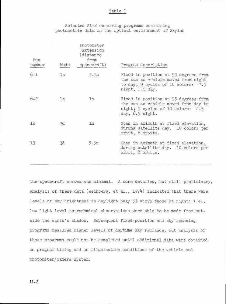
Table 1

Selected SL-2 observing programs containingphotometric data on the optical environment of Skylab

Runnumber

6-1

6-2

12

13

Mode

la

la

PhotometerExtension(distance

fromspacecraft)

5.5m

1m

Program description

Fixed in position at 95 degrees fromthe sun as vehicle moved from nightto day; 9 cycles of 10 colors: 7-5night, 1.5 day.

Fixed in position at 95 degrees fromthe sun as vehicle moved from day tonight; 9 cycles of 10 colors: 2.5day, 6.5 night.

Scan in azimuth at fixed elevation,during satellite day. 10 colors perorbit, 8 orbits.

Scan in azimuth at fixed elevation,during satellite day. 10 colors perorbit, 8 orbits.

the spacecraft corona was minimal. A more detailed, but still preliminary,

analysis of these data (Weinberg, et al., 197*0 indicated that there were

levels of sky brightness in daylight only 5$> above those at night; i.e.,

low light level astronomical observations were able to be made from out-

side the earth's shadow. Subsequent fixed-position and sky scanning

programs measured higher levels of daytime sky radiance, but analysis of

those programs could not be completed until additional data were obtained

on program timing and on illumination conditions of the vehicle and

photometer/camera system.

H-2

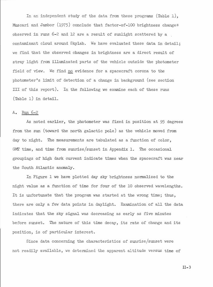
In an independent study of the data from these programs (Table l),

Muscari and Jambor (1975) conclude that factor-of-100 brightness changes

observed in runs 6-2 and 12 are a result of sunlight scattered by a

contaminant cloud around Skylab. We have evaluated these data in detail;

we find that the observed changes in brightness are a direct result of

stray light from illuminated parts of the vehicle outside the photometer

field of view. We find no evidence for a spacecraft corona to the

photometer's limit of detection of a change in background (see section

III of this report). In the following we examine each of these runs

(Table l) in detail.

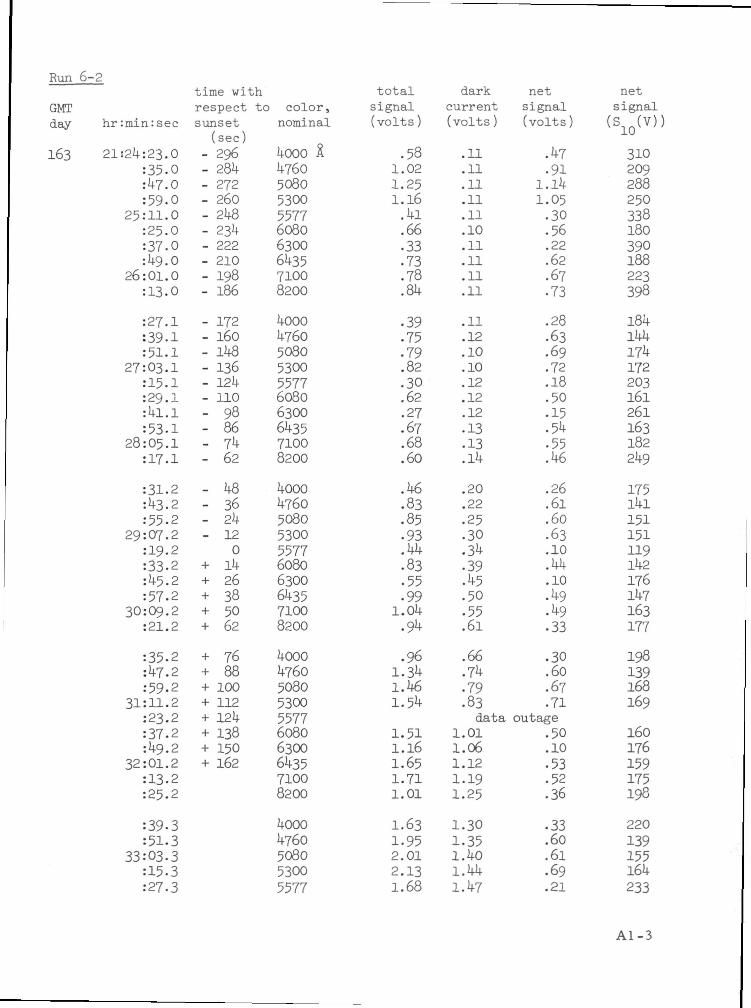
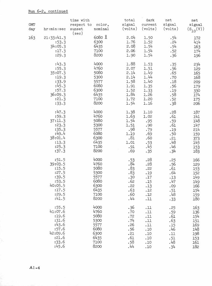
A. Run 6-2

As noted earlier, the photometer was fixed in position at 95 degrees

from the sun (toward the north galactic pole) as the vehicle moved from

day to night. The measurements are tabulated as a function of color,

GMT time, and time from sunrise/sunset in Appendix 1. The occasional

groupings of high dark current indicate times when the spacecraft was near

the South Atlantic anomaly.

In Figure 1 we have plotted day sky brightness normalized to the

night value as a function of time for four of the 10 observed wavelengths.

It is unfortunate that the program was started at the wrong time; thus,

there are only a few data points in daylight. Examination of all the data

indicates that the sky signal was decreasing as early as five minutes

before sunset. The nature of this time decay, its rate of change and its

position, is of particular interest.

Since data concerning the characteristics of sunrise/sunset were

not readily available, we determined the apparent altitude versus time of

II-3

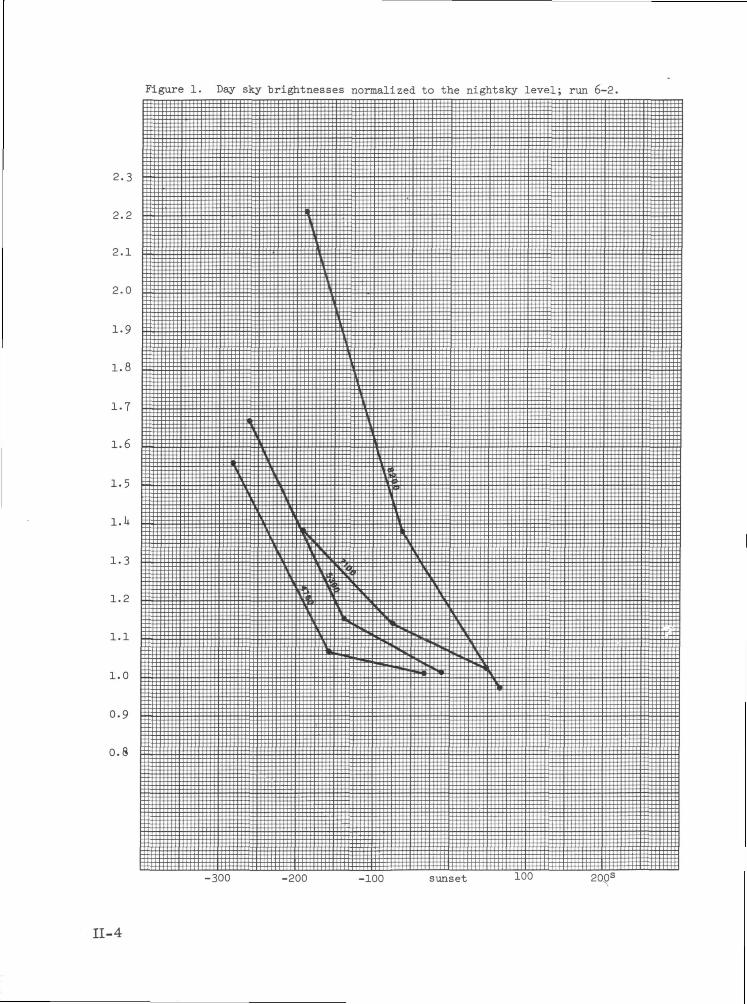
Figure 1. Day sky brightnesses normalized to the nightsky level; run 6-2.

2.3

2.2

2.1

2.0

1.0

0.9

0.8

-300 -200

II-4

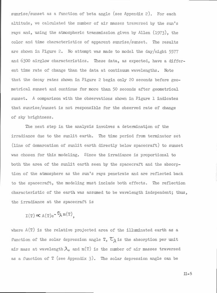
sunrise/sunset as a function of beta angle (see Appendix 2). For each

altitude, we calculated the number of air masses traversed by the sun's

rays and, using the atmospheric transmission given by Allen (l973)> the

color and time characteristics of apparent sunrise/sunset. The results

are shown in Figure 2. Ho attempt was made to model the day /night 5577

and 6300 airglow characteristics. These data, as expected, have a differ-

ent time rate of change than the data at continuum wavelengths . Note

that the decay rates shown in Figure 2 begin only 20 seconds before geo-

metrical sunset and continue for more than 50 seconds after geometrical

sunset. A comparison with the observations shown in Figure 1 indicates

that sunrise/sunset is not responsible for the observed rate of change

of sky brightness.

The next step in the analysis involves a determination of the

irradiance due to the sunlit earth. The time period from terminator set

(line of demarcation of sunlit earth directly below spacecraft) to sunset

was chosen for this modeling. Since the irradiance is proportional to

both the area of the sunlit earth seen by the spacecraft and the absorp-

tion of the atmosphere as the sun's rays penetrate and are reflected back

to the spacecraft, the modeling must include both effects. The reflection

characteristic of the earth was assumed to be wavelength independent; thus,

the irradiance at the spacecraft is

where A(T) is the relative projected area of the illuminated earth as a

function of the solar depression angle T, "C^ is the absorption per unit

air mass at wavelength A, and m(T) is the number of air masses traversed

as a function of T (see Appendix 3). The solar depression angle can be

H-5

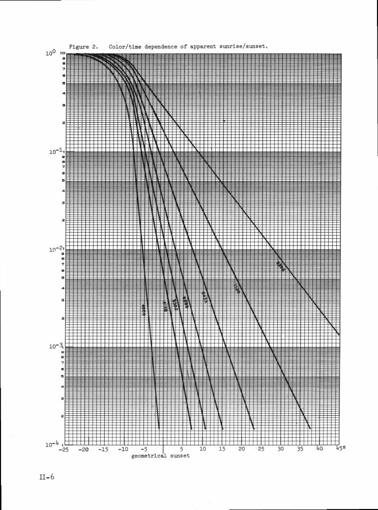
Figure 2. Color/time dependence of apparent sunrise/sunset

10-1* i-25 -20 -15 -10 -5 5 10 15 20 25 30 35 U5S

geometrical sunset

II-6

related to time through the orbital angular velocity and beta angle,

and thus the relative irradiance can be determined as a function of time.

The result is plotted in Figure 3 for the beta angle during Run 6-2.

As in the case of direct sunrise modeling, the effect on the airglow

lines was not considered.

As in Figure 2, there is a strong wavelength dependence in the time

decay characteristic. Note that a significant rate of decay is occurring

as early as 300 seconds before sunset and that the blue end of the

spectrum is diminished before the red end by as much as 50 to 100 seconds

before sunset. The similarity of these time characteristics to the observed

decay rates (Figure l) suggests strongly that the sunlit earth is the pri-

mary source of the observed changes.

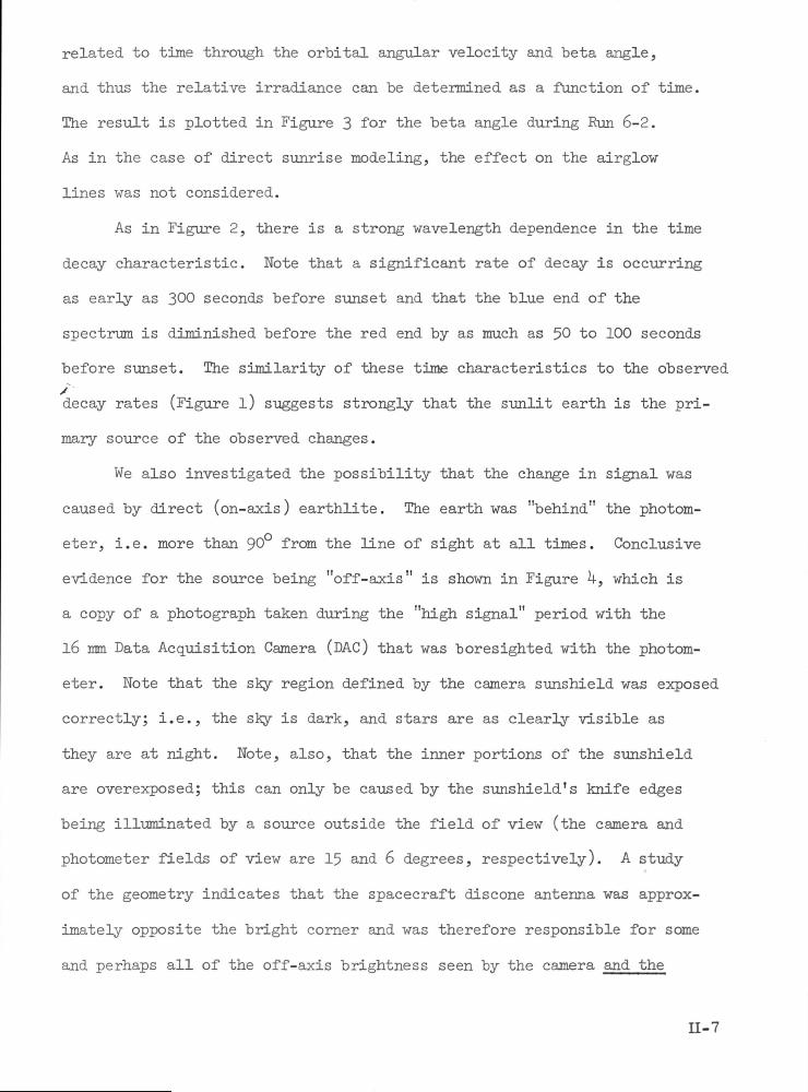
We also investigated the possibility that the change in signal was

caused by direct (on-axis) earthlite. The earth was "behind" the photom-

eter, i.e. more than 90° from the line of sight at all times. Conclusive

evidence for the source being "off-axis" is shown in Figure k, which is

a copy of a photograph taken during the "high signal" period with the

16 mm Data Acquisition Camera (DAC) that was boresighted with the photom-

eter. Note that the sky region defined by the camera sunshield was exposed

correctly; i.e., the sky is dark, and stars are as clearly visible as

they are at night. Note, also, that the inner portions of the sunshield

are overexposed; this can only be caused by the sunshield's knife edges

being illuminated by a source outside the field of view (the camera and

photometer fields of view are 15 and 6 degrees, respectively). A study

of the geometry indicates that the spacecraft discone antenna was approx-

imately opposite the bright corner and was therefore responsible for some

and perhaps all of the off-axis brightness seen by the camera and the

II-7

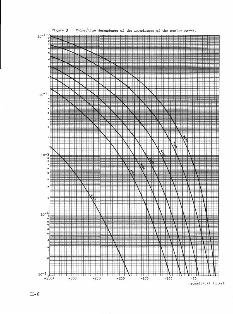
Figure 3. Color/time dependence of the irradiance of the sunlit earth.

10-

10-5-350S -300 -250 -200 -150 -100 -50

geometrical sunset

II-8

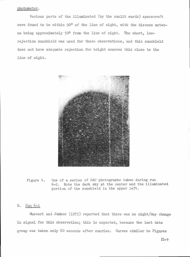
photometer.

Various parts of the illuminated (by the sunlit earth) spacecraft

were found to be within 90° of the line of sight, with the discone anten-

na being approximately 50° from the line of sight. The short, low-

rejection sunshield was used for these observations, and this sunshield

does not have adequate rejection for bright sources this close to the

line of sight.

Figure U. One of a series of DAC photographs taken during run6-2. Note the dark sky at the center and the illuminatedportion of the sunshield in the upper left.

B. Run 6-1

Muscari and Jambor (1975) reported that there was no night/day change

in signal for this observation; this is expected, because the last data

group was taken only 60 seconds after sunrise. Curves similar to Figures

n-9

2 and 3 for sunrise show that significant earthlight was not present

until more than 100 seconds after sunrise. Full direct sunlight was

present within 20 seconds after sunrise.

C. Run 12

The analysis of these data are more complex, because the photometer

was scanning in azimuth (i.e., in a plane approximately perpendicular to

the direction to the sun) during the measurement cycle. In this program

the photometer observed over a range of azimuth at fixed elevation; the

scan was made in a particular color, the photometer retraced its scan at

the next color, etc., until all 10 colors were used. The photometer then

waited until it reached the same starting place in the next orbit and it

repeated the cycle. Multicolor scans of a 60° region of azimuth were

obtained in this program on successive orbits, some scans with the

photometer 1 m from the spacecraft and some (run 13) at 5-5 m from the

spacecraft.

As noted by Muscari and Jambor (l975)> each scan was started (and

completed) during spacecraft day. The program was initiated only 11

seconds after sunrise, however; in orbit 1 it stopped at sunrise plus

110 seconds and in orbits 2 and 3 it stopped at sunrise plus 182 seconds.

This difference was due to. an anomaly in the instrument preparation rou-

tine; in the first orbit only the last 5 filters were used. This differ-

ence is important since the 8200A data in orbit 1 were taken starting

only 80 seconds after sunrise; in orbits 2 and 3 these data were taken

starting 150 seconds after sunrise. This is the filter that showed the

largest rise in signal, and these are the data that Muscari and Jambor

use to determine the level of "contamination".

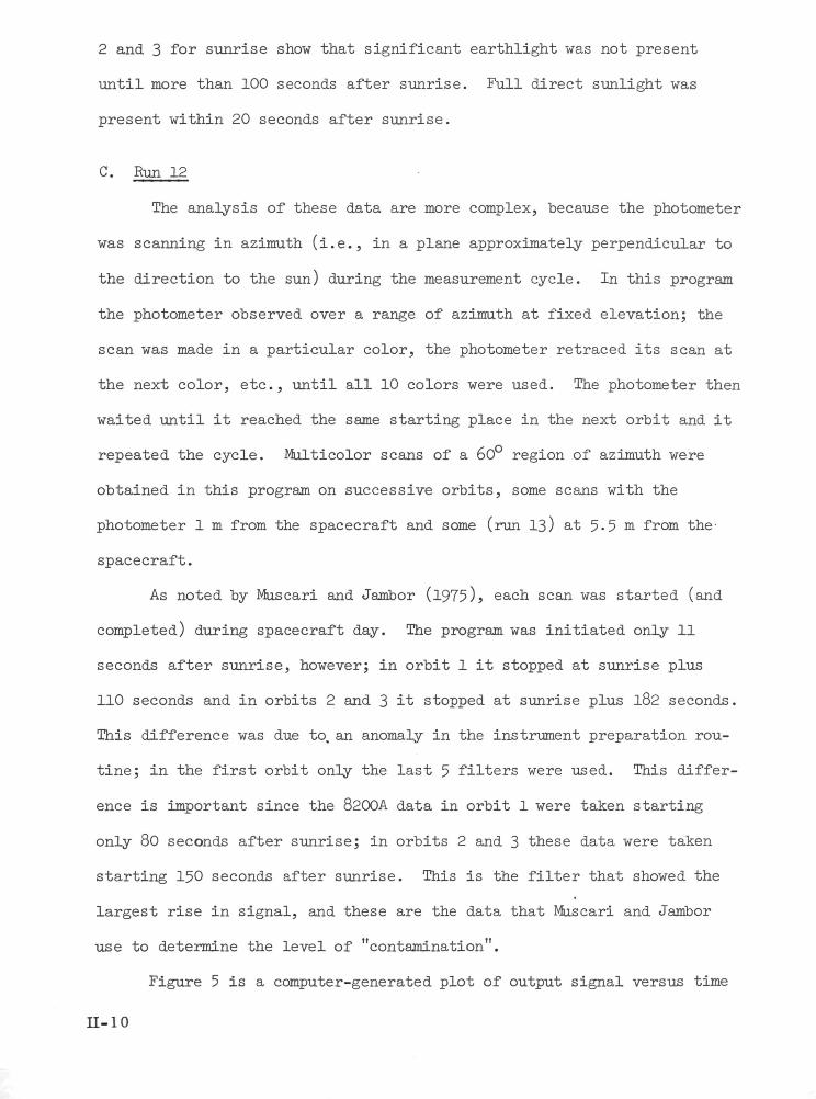
Figure 5 is a computer-generated plot of output signal versus time

11-10

RUN (2, ORBIT2

<n m in o ^s fi a-ifl mtf>N r o w r o c r i j - u i v D »—M * •!9N'Q~: — DIRECTION) OF e . ~ 0 -

^ C &• 6 mf!

12, OR6IT3

U5cr-u>

SMT sec -HBO' +151" *i&2" -HS?"UJITH RESPECT TD

5

11-11

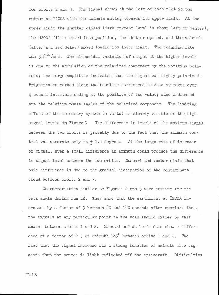
for orbits 2 and 3- The signal shown at the left of each plot is the

output at 7100A with the azimuth moving towards its upper limit. At the

upper limit the shutter closed (dark current level is shown left of center),

the 8200A filter moved into position, the shutter opened, and the azimuth

(after a 1 sec delay) moved toward its lower limit. The scanning rate

was 3-87 /sec. The sinusoidal variation of output at the higher levels

is due to the modulation of the polarized component by the rotating pola-

roid; the large amplitude indicates that the signal was highly polarized.

Brightnesses marked along the baseline correspond to data averaged over

• -second intervals ending at the position of the value; also indicated

are the relative phase angles of the polarized component. The limiting

effect of the telemetry system (5 volts) is clearly visible on the high

signal levels in Figure 5. The difference in levels of the maximum signal

between the two orbits is probably due to the fact that the azimuth con-

trol was accurate only to + l.k degrees. At the large rate of increase

of signal, even a small difference in azimuth could produce the difference

in signal level between the two orbits. Muscari and Jambor claim that

this difference is due to the gradual dissipation of the contaminant

cloud between orbits 2 and 3«

Characteristics similar to Figures 2 and 3 were derived for the

beta angle during run 12. They show that the earthlight at 8200A in-

creases by a factor of 3 between 80 and 1^0 seconds after sunrise; thus,

the signals at any particular point in the scan should differ by that

amount between orbits 1 and 2. Muscari and Jambor's data show a differ-

ence of a factor of 2.5 at azimuth 185° between orbits 1 and 2. The

fact that the signal increase was a strong function of azimuth also sug-

gests that the source is light reflected off the spacecraft. Difficulties

11-12

in the telemetry system require that the raw azimuth data be corrected.

When these corrections are made, the signal increases as a function of

azimuth for orbits 2 and 3 are almost identical, not significantly differ-

ent as indicated by Muscari and Jambor. Other differences noted by

Muscari and Jambor, especially the spectral differences, can also be

shown to be similar to the earthlight color/time characteristics.

The difference in direction of polarization of the enhanced signal

(Figure 5) is still further evidence against contamination as the source

of the enhancement. The direction of polarization for the zodiacal light

or for scattering by participates near the spacecraft is the same - perpen-

dicular to the direction to the sun. Only multiply-scattered light

(e.g., light scattered off the vehicle and seen by the sunshield baffles)

can give a different direction of polarization.

In summary, there is firm evidence for stray light from the sunlit

earth in the SL-2 photometer observations analyzed by Muscari and Jambor

(1975); we find no evidence for a detectable spacecraft corona in these

observations. In the subsequent section we show further that the photometer

would not detect the column brightness from the typical level of particu-

lates observed by the S052 coronagraph.

References

C. W. Allen, Astrophysical Quantities, 3rd edition, the Athlone Press, 1973-

J. A. Muscari and B. Jambor, Final Report, Skylab Experiment T027,ED-2002-1776, Martin-Marietta, June 1975-

J. L. Weinberg, R. D. Mercer, and R. C. Hahn, The optical environment ofSkylab, Mission SL-2, Bull. AAS, 6, 337,

11-13

III. The Composite Picture

Photographs obtained with the S052 coronagraph and photoelectric

data obtained with the photometer of experiments S073 and T027 contain

unique data on the Skylab spacecraft corona. Particle tracks on the S052

photographs have provided data on discrete contaminant particulates at

small scattering angles: number, size, distance, velocity. Further

analysis of selected photometric data from Mission SL-2 showed no evidence

for integrated light from contaminant particulates down to our threshold

of detection of a few S- V) . It is of interest to determine the approx-

imate sensitivity of the photometer to the brightness contributed by

individual particles and to compare the photographic (small angle) and

photoelectric (large angle) results.

We make the following assumptions:

1. The average particle size 0 is 25 microns in radius;

2. The particles are uniformly distributed out to a distanceL of 200 meters from the spacecraft;

3- The energy scattered from each particle at scatteringangles of 90° 1 10° is .05 of the energy of an isotropicscatterer whose scattering cross section is assumed to beequivalent to its geometrical cross section.

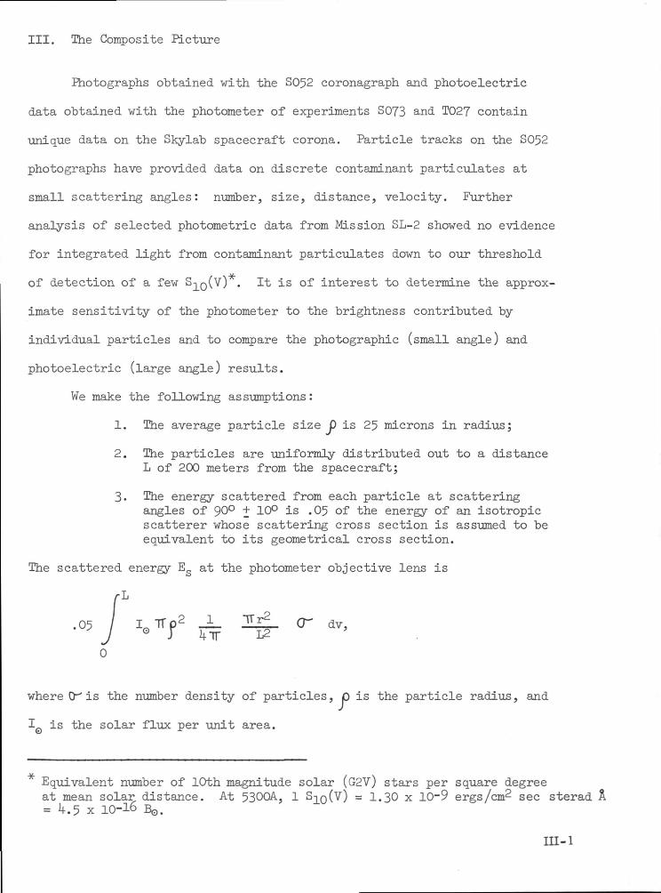
The scattered energy Eg at the photometer objective lens is

-L

.05 / I0TTp2 1 -!!£- 0- dv,J 4TT I£

0

where 0^ is the number density of particles, O is the particle radius, and

I0 is the solar flux per unit area.

Equivalent number of 10th magnitude solar (G2V) stars per square degreeat mean solar distance. At 5300A, 1 S10(v) = 1-30 x 10-9 ergs/cm

2 sec sterad A= IK5 x 10-16 BQ.

m-i

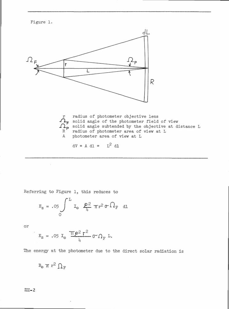
Figure 1.

radius of photometer objective lenssolid angle of the photometer field of view

-O-p solid angle subtended by the objective at distance Lradius of photometer area of view at LRphotometer area of view at L

dV = A dl = L2 dl

Referring to Figure 1, this reduces to

or

ES = .05 1

The energy at the photometer due to the direct solar radiation is

B0 IT r2

III-2

or

/lo

Normalizing the radiation from the particles to the direct solar radiation

gives

.05 i0 _ cr

G

Using the values assumed earlier for D and L and the solid anglelio oft~7

the sun, we obtain 1.06 x 10"'fl~.

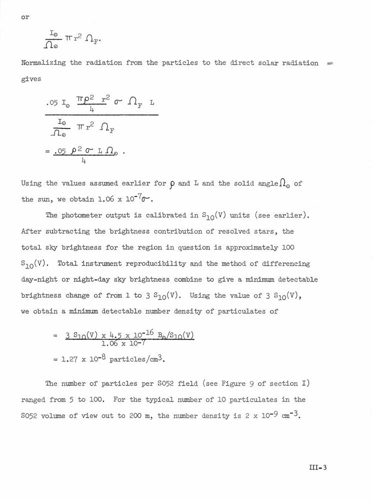
The photometer output is calibrated in S- Q(V) units (see earlier).

After subtracting the brightness contribution of resolved stars, the

total sky brightness for the region in question is approximately 100

SJLQ(V). Total instrument reproducibility and the method of differencing

day-night or night-day sky brightness combine to give a minimum detectable

brightness change of from 1 to 3 SJ_Q(V). Using the value of 3

we obtain a minimum detectable number density of particulates of

= 3 Sin(v) x k 5 x IP"l6

1.06 x 10-7

= 1.27 x 10"° particles/cm3.

The number of particles per S052 field (see Figure 9 of section I)

ranged from 5 to 100. For the typical number of 10 particulates in the

S052 volume of view out to 200 m, the number density is 2 x 10~9 cm~3.

HI-3

Our inability to distinguish a day-night or night-day change in brightness

which could be attributed to contamination is therefore consistent with

the S052 analysis which finds the typical number density to be below our

-column brightness threshold for detection. However, there were periods

of a factor-of-ten higher concentration that would bring the particulate

background up to the level of detectability of the photometer. Since

this increased level of participates had no preferred direction, we do

not associate these levels with dumps or thruster firings.

Ill-4

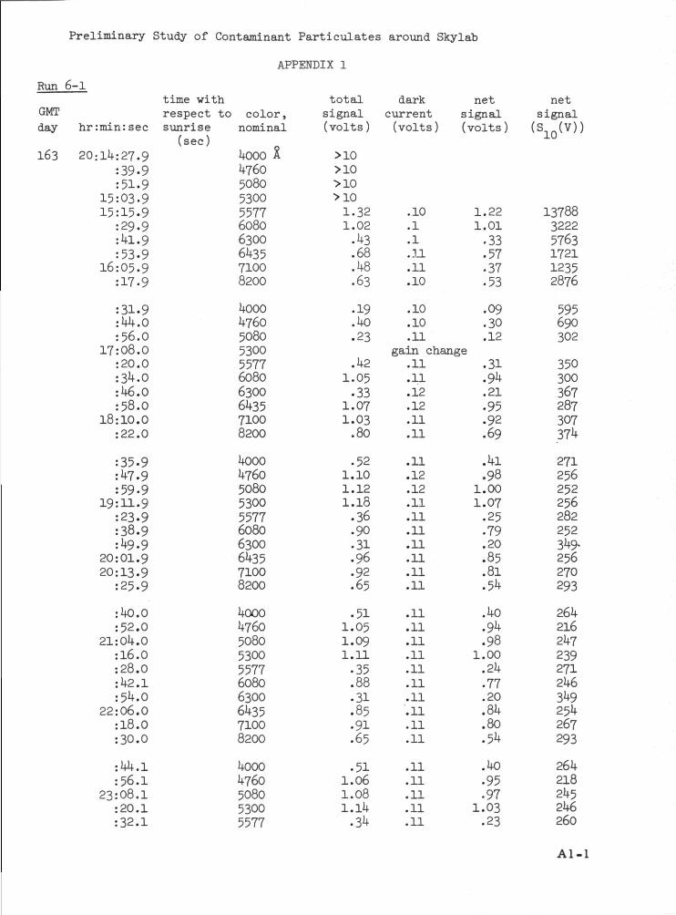
Preliminary Study of Contaminant Particulates around Skylab

APPENDIX 1

Run 6-1

GMTday hr:min:sec

163 20:ll+:27.9:39-9:51.9

15:03-915:15.9

:29-9:Ul.9:53.9

16:05.9:17«9

:31.9:M+.0:56.0

17:08.0:20.0:3^-0:1+6.0:58.0

18:10.0:22.0

:35-9:Vf.9:59-9

19:11.9:23.9:38.9:^9.9

20:01.920:13.9

:25.9

:1+0.0:52.0

21:0l+.0:l6.0:28.0: 1*2.1:5l+.0

22:06.0:18.0:30.0

:Wt.l:56.1

23:08.1:20.1:32.1

time withrespect to color,sunrise nominal

(sec)1+000 Ai+7605080530055776080630061+3571008200

1*000U7605080530055776080630061+3571008200

Uooo1+7605080530055776080630061+3571008200

1+0001+7605080530055776080630061+3571008200

1+0001+760508053005577

totalsignal(volts)

>10>10>10>10

1.321.02

.U3

.68

.1+8

.63

.19

.1+0

.23

darkcurrent

(volts)

.10

.1

.1

.11

.11

.10

.10

.10

.11

netsignal(volts)

1.221.01

.33

.57

.37

.53

• 09.30.12

netsignal

( s i n (v ) )10

1378832225763172112352876

595690302

gain change.1+2

1.05.33

1.071.03

.80

.521.101.121.18

.36• 90• 31• 96.92.65

.511.051.091.11

• 35.88.31.85.91.65

• 511.061.081.11+.3*

.11

.11

.12

.12

.11

.11

.11

.12

.12

.11

.11

.11

.11

.11

.11

.11

.11

.11

.11

.11

.11

.11

.11

.11

.11

.11

.11

.11

.11

.11

.11

.31

.9*

.21• 95.92.69

.1+1

.981.001.07

.25

.79

.20

.85

.81

.ft

.1+0

.9*

.981.00

.21+

.77

.20

.81+

.80

.5U

.1+0

• 95• 97

1.03.23

350300367287307371+

27125625225628225231+9-256270293

261+2162l+72392712l+63^9251+267293

261+2182l+521+6260

Al-1

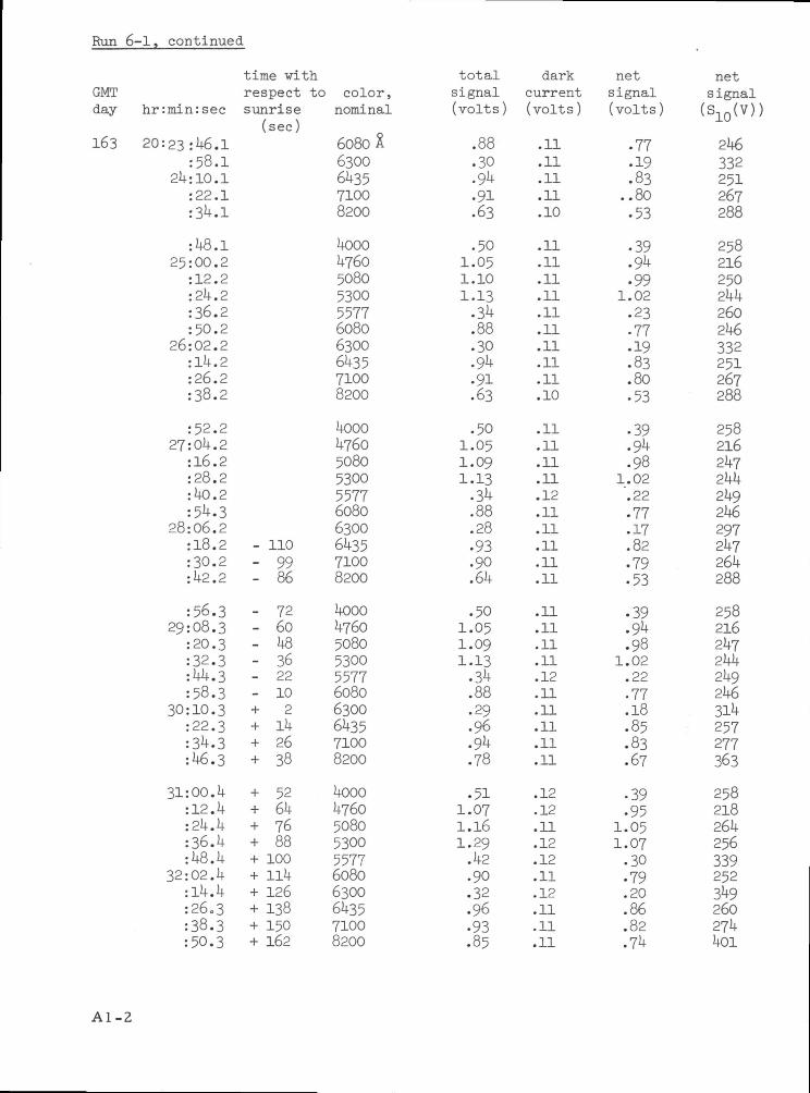
Run 6-1, continued

GMTday

163

hr:min:sec

20:23:46.1:58.1

24:10.1:22.1:34.1

:48.125:00.2:12.2:24.2:36.2:50.2

26:02.2:l4.2:26.2:38.2

:52.227:04.2:l6.2:28.2:40.2:54.3

28:06.2:18.2:30.2:42.2

:56.329:08.3

:20.3:32.3:44.3:58.3

30:10.3:22.3:34.3:46.3

31:00.4:12.4:24.4:36.4:48.4

32:02.4:14.4:26.3:38.3:50.3

- 110- 99- 86

- 72- 60- 48- 36- 22- 10+ 2+ 14+ 26+ 38

+ 52+ 64+ 76+ 88+ 100+ n4+ 126+ 138+ 150+ 162

time withrespect to color,sunrise nominal

(sec)6080 A

6300643571008200

4ooo476050805300557760806300643571008200

4ooo476050805300557760806300643571008200

4ooo476050805300557760806300643571008200

4ooo476050805300557760806300643571008200

totalsignal(volts)

.88• 30.9*.91.63

.501.051.101.13.34.88.30.94• 91.63

.501.051.091.13.34.88.28.93.90.64

.501.051.091.13• 34.88• 29.96• 94.78

• 511.0?1.161.29.42.90.32.96.93.85

darkcurrent(volts)

.11

.11

.11

.11

.10

.11

.11

.11

.11

.11

.11

.11

.11

.11

.10

.11

.11

.11

.11

.12

.11

.11

.11

.11

.11

.11

.11

.11

.11

.12

.11

.11

.11

.11

.11

.12

.12

.11

.12

.12

.11

.12

.11

.11

.11

netsignal(volts)

.77

.19

.83..80.53

.39

.94• 99

1.02.23• 77.19.83.80• 53

.39

.94

.981.02'.22• 77.17.82.79.53

• 39.94.98

1.02.22.77.18.85.83.67

• 39• 95

1.051.07• 30• 79.20.86.82.74

netsignal(s10(v))

21*6332251267288

258216250244260246332251267288

258216247244249246297247264288

258216247244249246314257277363

2582182642563392523492602744oi

Al-2

Run 6-2time with

GMTday hr:min:sec

163 21:2l+:23.0:35.0: 1+7.0:59-0

25:11.0:25.0:37.0: 1+9.0

26:01.0:13.0

:27.1:39-l:51.1

27:03.1:15.1:29.1:1+1.1:53-l

28:05.1:!?.!

:31.2:l+3.2-.55-2

29:07.2:19.2:33-2;l+5.2:57.2

30:09.2:21.2

:35-2;l+7.2:59-2

31:11.2:23.2:37.2;l+9.2

32:01.2:13.2:25.2

:39-3:51.3

33:03.3:15.3:27-3

respectsunset

(sec)- 296- 281+- 272- 260- 2l+8- 231+- 222- 210- 198- 186

- 172- 160- 11+8- 136- 12l+- 110- 98- 86- 7l+- 62

1+8- 36- 21+- 12

0+ ll++ 26+ 38+ 50+ 62

+ 76+ 88+ 100+ 112+ 12l++ 138+ 150+ 162

to color,nominal

1+000 X1+7605080530055776080630061+3571008200

1+0001+7605080530055776080630061+3571008200

1+0001+7605080530055776080630061+3571008200

1+0001+7605080530055776080630061+3571008200

1+0001+760508053005577

totalsignal(volts)

.581.021.251.16

.1+1

.66

.33

.73

.78

.81+

.39

.75

.79

.82

.30

.62

.27

.67

.68

.60

.1+6

.83

.85

.931+1+

.83• 55• 99

l.OU• 9U

.961.3!+1.1+61.5*+

1.511.161.651.711.01

1.631.952.012.131.68

darkcurrent(volts)

.11

.11

.11

.11

.11

.10

.11

.11

.11

.11

.11

.12

.10

.10

.12

.12

.12

.13

.13

.11+

.20

.22

.25• 30• 3^.39.1+5.50.55.61

.66

.71+

.79

.83data

1.011.061.121.191.25

1.301.351.1+01.1+1+1.1+7

netsignal(volts)

.1+7

.911.11+1.05

.30

.56

.22

.62

.67• 73

.28

.63

.69

.72

.18

.50

.15

.51+• 55.1+6

.26

.61

.60

.63

.10

.1+1+

.10A9.1+9.33

.30

.60

.67

.71outage

.50

.10• 53.52.36

• 33.60.61.69.21

netsignal(sio(v))

310209288250338180390188223398

184

17!+172203161261163182

175llU151151119

176

163177

198139168169

160176159175198

220

139155161+233

Al-3

Run 6-2, continued

GMTday hr:min:sec

163 21:33: 1.3:53-3

3 :05.3:17.3:29-3

:l*3-3= 55.3

35:07.3:19-3:33-9:l*5-3:57.3

36:09.3:21.3:33.3

:1*7.3:59-3

37:11.3:23-3:35.3:1*9.1*

38:01.1*:13.3:25.3:37.3

:51.539:03.5

:15.5:27.5:39-5:53.5

1*0:05.5:17.5:29.5:1*1.5

:55.51*1:07.6:19.6:31.6:1*3.6:57.6

1*2:09.6:21.6:33-6= 1*5.6

time withrespect to color,sunset nominal(sec)

6080 A630061*3571008200

1*0001*7605080530055776080630061*3571008200

1*0001*7605080530055776080630061*3571008200

1*0001*7605080530055776080630061*3571008200

1*0001*7605080530055776080630061*3571008200

totalsignal(volts)

2.0l*1.762.082.061.90

1.882.072.1k2.1k1.581.911.521.81*1.721.51*

1.381.631.51*1.51.98

1.19.811.01.91.69

.53

.81*

.83

.83

.30

.62

.22

.63

.60

.1*1*

.36

.70

.72

.71*

.26

.56

.21

.61

.58

.1*1*

darkcurrent(volts)

1.501.521.51*1.51*1.51*1.531.511.1*91.1*1*1.1*01.351.331.261.201.16

1.101.02• 95.90.79.69.60.53.1*5• 35

.28

.28

.22

.19

.17

.15

.13

.12

.12

.11

.11

.11

.11

.11

.11

.10

.10

.10

.10

.10

netsignal(volts)

• 5k.21*.51*• 52.36

• 35.56.65.70.18.56.19.58• 52.38

.28

.61

.59

.61

.19

.50

.21

.1*8

.1*6

.3

.25

.56

.61

.64

.13

.1*7

.09

.51

.1*8

.33

.25

.59

.61

.63

.15

.1*6

.11

.51

.1*8

.34

netsignal(S (V))

J-U

1721*11*163171*196

23!*129165168209179330

175206

187ll*lll*8lk72lk159373ll*5153183

166129153152ll*9li*9166151*159180

163136151*151169ll*8198153161182

Al-4

Preliminary Study of Contaminant Particulates around Skylab

APPENDIX 2

sun

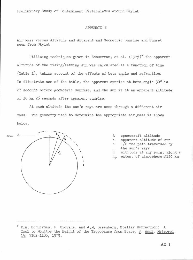
Air Mass versus Altitude and Apparent and Geometric Sunrise and Sunsetseen from Skylab

Utilizing techniques given in Schuerman, et al. (1975) the apparent

altitude of the rising/setting sun was calculated as a function of time

(Table l), taking account of the effects of beta angle and refraction.

To illustrate use of the table, the apparent sunrise at beta angle 30° is

27 seconds before geometric sunrise, and the sun is at an apparent altitude

of 10 km 26 seconds after apparent sunrise.

At each altitude the sun's rays are seen through a different air

mass. The geometry used to determine the appropriate air,mass is shown

below.

A spacecraft altitudeh apparent altitude of suns 1/2 the path traversed by

the sun's raysH altitude at any point along shm extent of atmosphere~120 km

D.W. Schuerman, F. Giovane, and J.M. Greenberg, Stellar Refraction: ATool to Monitor the Height of the Tropopause from Space, J. Appl. Meteorol.lU, 1182-1186, 1975-

A2-1

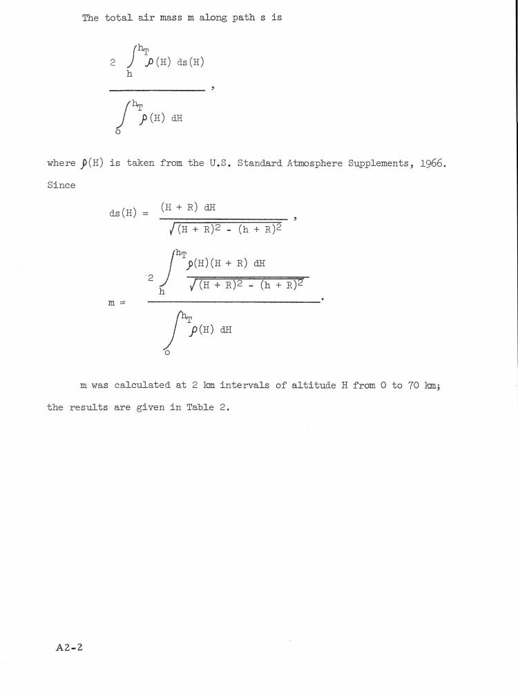
The total air mass m along path s is

2 J JD(H) ds(H)h

dH

where J>(H) is taken from the U.S. Standard Atmosphere Supplements, 1966.

Since

/(H + R)2 - (h + R)2

+ R) dH

m =

JD(H) dH

o

m was calculated at 2 km intervals of altitude H from 0 to 70 km;

the results are given in Table 2.

A2-2

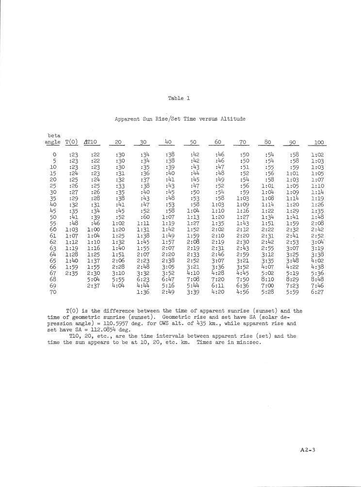
Table 1

Apparent Sun Rise/Set Time versus Altitude

betaangle T(0) 4T10 20 30 1*0 50 60 70 80 90 100

05

101520253035i+oU550556061626361+656667686970

= 23:23:23:2l+:25:26:27:29:32:35:lU:U8

1:031:071:121:191:281:1*01:592:35

:22:22:23:23:2l*:25:26:28:31:3l*= 39:k6

1:001:01+1:101:161:251:371:552:305:0l*2:37

:30:30:30:31:32:33:35:38:Ul:^5:52

1:021:201:251:321:1*01:512:062:283:105:55l*:0l*

:3l*:3l*:35:36:37:38:1*0:1*3:kl:52:60

1:111:311:381:1*51:552:072:232:1*83:326:231*:1*1*1:36

:38:38:39:1*0:1*1:1*3:^5:1*8:53:58

1:071:191:1*21:1*91:572:072:202:383:053:526:1*75:162:1*9

:U2:l+2:^3;1*1*:l+5•M:50:53:58

1:01*1:131:271:521:592:082:192:332:523:211*:107:085:M*3:39

:1*6.-1*6:1*7;1*8= 1*9:52:5^:58

1:031:101:201:352:022:102:192:312:1*63:073:361*:287:206:111*:20

:50:50:51:52:5U:56:59

1:031:091:161:271*32:122:202:302:1*32:593:213:52l+:l+57:506:361*:56

:5l*:5U:55:56:58

1:01l:0l*1:08l:ll*1:221:31*1:512:222:312:1*22:553:123:351*:075:028:107:005:28

:58= 58:59

1:011:031:051:09l:ll*1:201:291:1*11:592:322:1*12:533:073:253:1*81*:225:198:297:235:59

1:021:031:031:051:071:10l:ll*1:191:261:351:1*82:082:1*22:523:01*'3:193:381*:021*:385:368:1*87:1*66:27

T(0) is the difference between the time of apparent sunrise (sunset) and thetime of geometric sunrise (sunset). Geometric rise and set have SA (solar de-pression angle) = 110.5957 deg. for OWS alt. of 1*35 km-, while apparent rise andset have SA = 112.085!* deg.

T10, 20, etc., are the time intervals between apparent rise (set) and thetime the sun appears to be at 10, 20, etc. km. Times are in min:sec.

A2-3

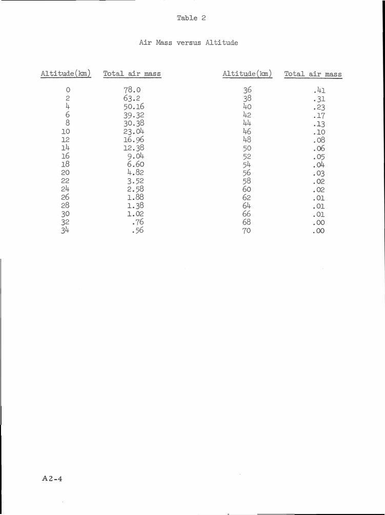
Table 2

Air Mass versus Altitude

Altitude(km) Total air mass Altitude(km) Total air mass

02

68

1012111161820222k26283032

78.063.250.1639-3230.3823. ok16.9612.38

ok,60

k.825258883802

.76

.56

3638ItOk2kkk6kQ5052

565360626k666870

.31

.23

.17

.13

.10

.08

.06

.05

.Ok

.03

.02

.02

.01

.01

.01

.00

.00

A2-4

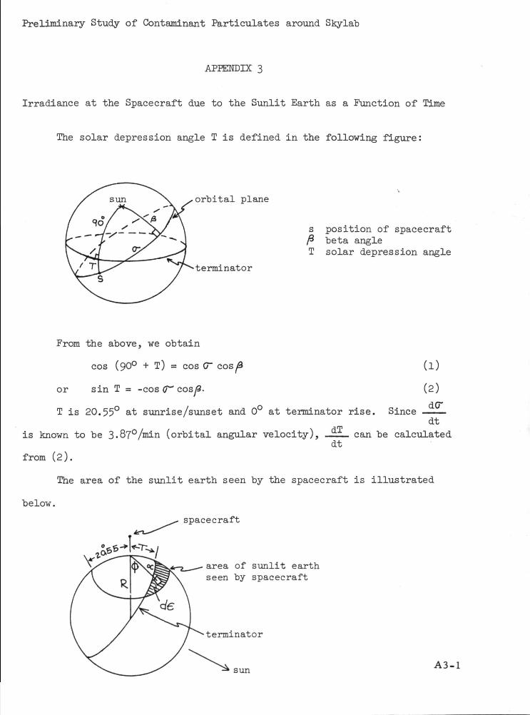
Preliminary Study of Contaminant Particulates around Skylab

APPENDIX 3

Irradiance at the Spacecraft due to the Sunlit Earth as a Function of Time

The solar depression angle T is defined in the following figure:

orbital plane

terminator

s position of spacecraftft beta angleT solar depression angle

From the above, we obtain

cos (90° + T) = cos G~

or sin T = -cos (T cosl3.

T is 20.55° at sunrise/sunset and 0° at terminator rise. Since

(1)

(2)

dO"

dtis known to be 3.87°/min (orbital angular velocity), __— can be calculated

dtfrom (2).

The area of the sunlit earth seen by the spacecraft is illustrated

below.

spacecraft

area of sunlit earthseen by spacecraft

terminator

sun A3-1

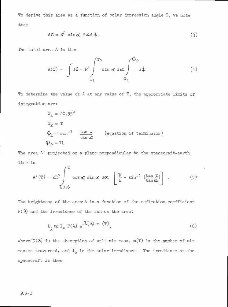
To derive this area as a function of solar depression angle T, we note

that

dG = R2 sinoC docd<£. (3)

The total area A is then

A(T) = [ d 6 = R 2 / sin oC dec I dd. (k)

Tl

To determine the value o'f A at any value of T, the appropriate limits of

integration are :

T! = 20.55°

T2 = T

d>-, = sin"1 tan T (equation of terminator)tanoc

The area A' projected on a plane perpendicular to the spacecraft-earth

line is

rA ' ( T ) = 2R2 I cosoC sin oC doc | £ - sin'1 (^2_Z) | . (5>

/0.6

inoC doc | - sin'1

The brightness of the area- A is a function of the reflection coefficient

and the irradiance of the sun on the area:

(6)

where'C(X) is the absorption of unit air mass, m(l) is the number of air

masses traversed, and IQ is the solar irradiance. The irradiance at the

spacecraft is then

A3-2

Is(T)oC BA A' e- m T (7)

or

I(T)oCA'(T) Ffr) Ie e-2CW ffi (T). (8)

is assumed to be a constant and IQ is known. Thus

Is(T)oC A'(T) e-2 m . (9)

The function m(T) can be determined from

cos(T + 26) = R cos 8 , (10)R + h

where Q is the solar elevation angle, R is the radius of the earth, and

h is the spacecraft altitude.

(T) is determined from (10) and m(e) is obtained from Allen (1973).

Therefore, m(T) is the product of the functions 9(T) and m(9), and IS(T)

can hp determined. Since T(t) can be determined from (2), Is(t) can be

A3-3NASA-Langley, 1976

WASHINGTON. D.C. 2O546

OFFICIAL BUSINESS

PENALTY FOR PRIVATE USE S3OO SPECIAL FOURTH-CLASS RATEBOOK

S ANDSPACE AOMINIS1RAT

451

POSTMASTER: If Undeliverable (Section 158Postiil Man iu i l ) Do Not Return

"The aeronautical and space activities of the United States shall beconducted so as to contribute . . . to the expansion of human knowl-edge of phenomena in the atmosphere and space. The Administrationshall provide for the widest practicable and appropriate disseminationof information concerning its activities and the results thereof."

—NATIONAL AERONAUTICS AND SPACE ACT OF 1958

NASA SCIENTIFIC AND TECHNICAL PUBLICATIONSTECHNICAL REPORTS: Scientific andtechnical information considered important,complete, and a lasting contribution to existingknowledge.

TECHNICAL NOTES: Information less broadin scope but nevertheless of importance as acontribution to existing knowledge.

TECHNICAL MEMORANDUMS:Information receiving limited distributionbecause of preliminary data, security classifica-tion, or other reasons. Also includes conferenceproceedings with either limited or unlimiteddistribution.

CONTRACTOR REPORTS: Scientific andtechnical information generated under a NASAcontract or grant and considered an importantcontribution to existing knowledge.

TECHNICAL TRANSLATIONS: Informationpublished in a foreign language consideredto merit NASA distribution in English.

SPECIAL PUBLICATIONS: Informationderived from or of value to NASA activities.Publications include final reports of majorprojects, monographs, data compilations,handbooks, sourcebooks, and specialbibliographies.

TECHNOLOGY UTILIZATIONPUBLICATIONS: Information on technologyused by NASA that may be of particularinterest in commercial and other non-aerospaceapplications. Publications include Tech Briefs,Technology Utilization Reports andTechnology Surveys.

Details on the availability of these publications may be obtained from:

SCIENTIFIC AND TECHNICAL INFORMATION OFFICE

A T I O N A L A E R O N A U T I C S A N D S P A C E A D M I N I S T R A T I O N

Washington, D.C. 20546