Preliminary Cruise Report Marine CSEM Surveys of Green … · Preliminary Cruise Report Marine CSEM...

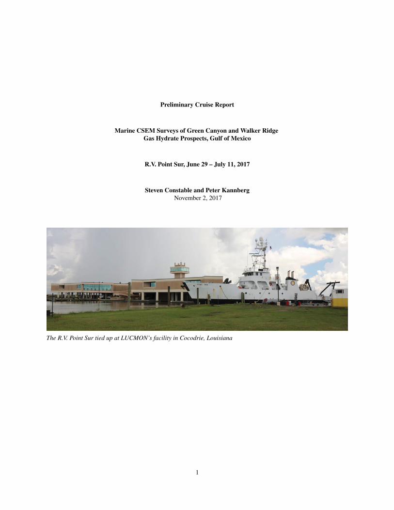
Preliminary Cruise Report

Marine CSEM Surveys of Green Canyon and Walker RidgeGas Hydrate Prospects, Gulf of Mexico

R.V. Point Sur, June 29 – July 11, 2017

Steven Constable and Peter KannbergNovember 2, 2017

The R.V. Point Sur tied up at LUCMON’s facility in Cocodrie, Louisiana

1

INTRODUCTION AND MOTIVATION

Current geophysical surveying methods for identifying seafloor gas hydrates, such as seismic methods and welllogging/coring, are limited in various ways. A characteristic seismic signature associated with hydrate is the bottom-simulating reflector (BSR). The BSR tracks the phase change of solid hydrate (above) and free gas (below) that iscontrolled by the intersection of the hydrate stability field with the local geothermal gradient. Because of this, theBSR usually tracks parallel to the sea floor and often cross-cuts sedimentary structures. However, the strong seismicsignature associated with traces of free gas at the BSR is almost completely independent of the amount of hydratehigher in the section. Seismic blanking and seismic bright spots may be a better indication of hydrate in the section,but reveal little about the thickness and concentration of the material. Well logging or coring, while providing locallydefinitive data, is expensive, invasive, and provides only a point measurement for the direct presence of hydrate.

Quantifying the volume fraction of hydrate in sediments is possible with careful processing and inversion of seismicdata, although the relationship between seismic velocity (or attenuation) and hydrate concentration is complicated.Electromagnetic methods, on the other hand, are sensitive to the concentration and geometric distribution of hydrate.Resistivity measurements made during well logging indicate that regions containing hydrate are significantly moreresistive when compared to water saturated zones, and direct laboratory measurement of methane hydrate confirms thatfully hydrate-saturated sands have a resistivity of about 2,000 Ωm, a thousand times higher than typical host sediments.

CRI P

PS I N

ST

I TU TION OF OCE ANOGRA

PHY

UCS D

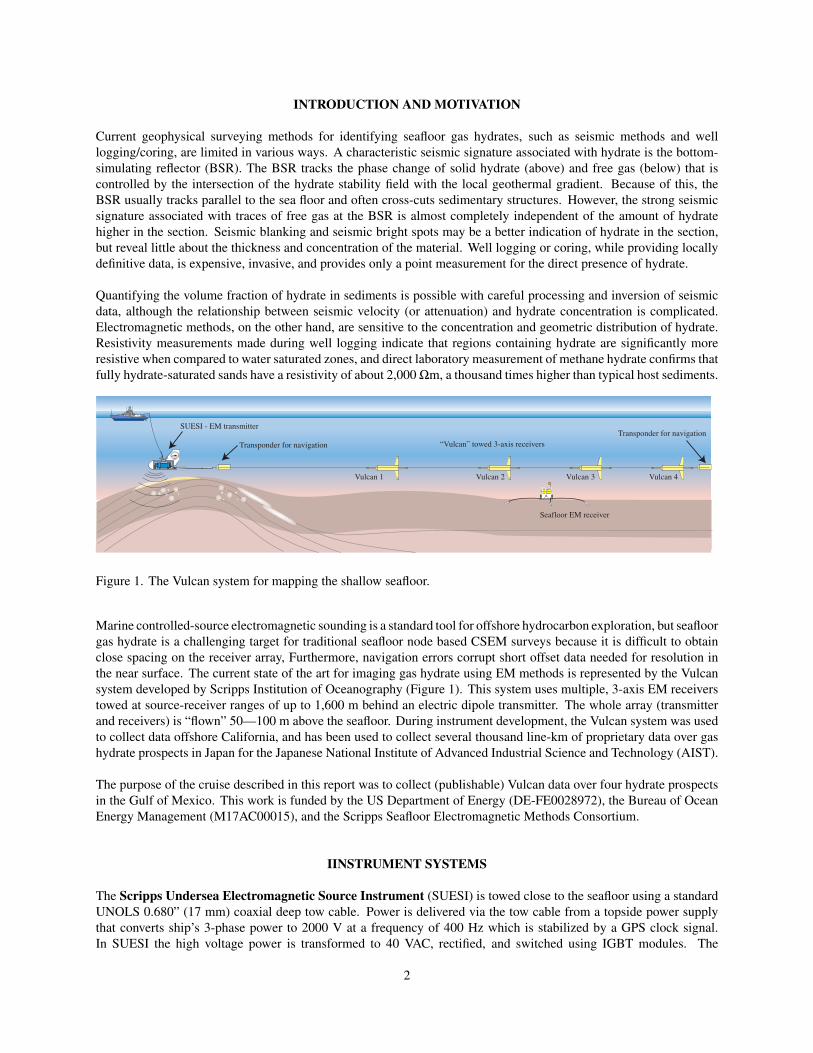
Transponder for navigationTransponder for navigation “Vulcan” towed 3-axis receivers

Vulcan 1 Vulcan 2 Vulcan 3 Vulcan 4

Seafloor EM receiver

SUESI - EM transmitter

Figure 1. The Vulcan system for mapping the shallow seafloor.

Marine controlled-source electromagnetic sounding is a standard tool for offshore hydrocarbon exploration, but seafloorgas hydrate is a challenging target for traditional seafloor node based CSEM surveys because it is difficult to obtainclose spacing on the receiver array, Furthermore, navigation errors corrupt short offset data needed for resolution inthe near surface. The current state of the art for imaging gas hydrate using EM methods is represented by the Vulcansystem developed by Scripps Institution of Oceanography (Figure 1). This system uses multiple, 3-axis EM receiverstowed at source-receiver ranges of up to 1,600 m behind an electric dipole transmitter. The whole array (transmitterand receivers) is “flown” 50—100 m above the seafloor. During instrument development, the Vulcan system was usedto collect data offshore California, and has been used to collect several thousand line-km of proprietary data over gashydrate prospects in Japan for the Japanese National Institute of Advanced Industrial Science and Technology (AIST).

The purpose of the cruise described in this report was to collect (publishable) Vulcan data over four hydrate prospectsin the Gulf of Mexico. This work is funded by the US Department of Energy (DE-FE0028972), the Bureau of OceanEnergy Management (M17AC00015), and the Scripps Seafloor Electromagnetic Methods Consortium.

IINSTRUMENT SYSTEMS

The Scripps Undersea Electromagnetic Source Instrument (SUESI) is towed close to the seafloor using a standardUNOLS 0.680” (17 mm) coaxial deep tow cable. Power is delivered via the tow cable from a topside power supplythat converts ship’s 3-phase power to 2000 V at a frequency of 400 Hz which is stabilized by a GPS clock signal.In SUESI the high voltage power is transformed to 40 VAC, rectified, and switched using IGBT modules. The

2

output waveform is a custom, compact binary signal that has 1–2 decades of usable frequencies, and is synchronizedusing the GPS stabilized 400 Hz power signal. Maximum output current is 500 A zero to peak, but on the smallertransmission antennas used for hydrate studies we are limited to 200–300 A. A frequency shift keyed (FSK) 9,600 baudbidirectional communication signal is overlain on the power transmission and allows SUESI navigation data (depth,altitude, water sound velocity, long baseline acoustics), operational information (input voltage, output voltage, outputcurrent, temperature throughout the system), and Vulcan telemetry (see below) to be monitored in real time. We canalso issue commands to set operation parameters and synchronize the output on the minute.

In this project we used a neutrally buoyant 100 m transmission antenna with an output current of about 260 A with afundamental frequency of 0.5 Hz. We carried full redundancy for the SUESI system on this cruise, with two SUESIunderwater systems, two topside power supplies, and two antenna arrays and winches. However, SUESI workedperfectly for this project and we did not need to substitute any equipment.

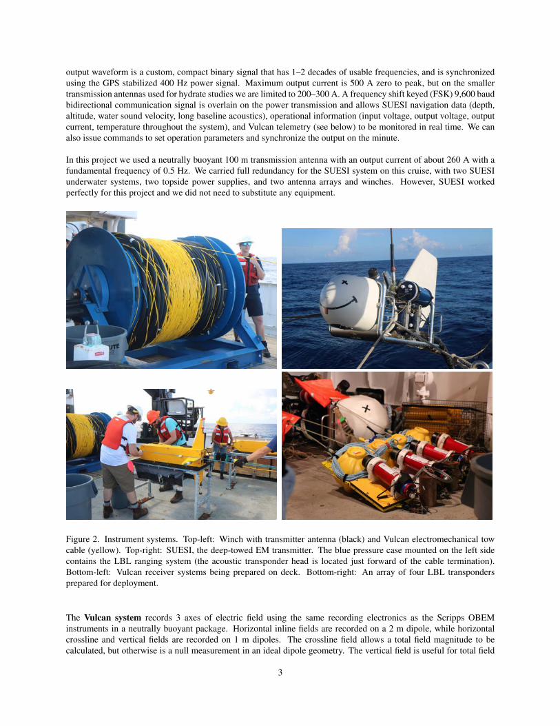
Figure 2. Instrument systems. Top-left: Winch with transmitter antenna (black) and Vulcan electromechanical towcable (yellow). Top-right: SUESI, the deep-towed EM transmitter. The blue pressure case mounted on the left sidecontains the LBL ranging system (the acoustic transponder head is located just forward of the cable termination).Bottom-left: Vulcan receiver systems being prepared on deck. Bottom-right: An array of four LBL transpondersprepared for deployment.

The Vulcan system records 3 axes of electric field using the same recording electronics as the Scripps OBEMinstruments in a neutrally buoyant package. Horizontal inline fields are recorded on a 2 m dipole, while horizontalcrossline and vertical fields are recorded on 1 m dipoles. The crossline field allows a total field magnitude to becalculated, but otherwise is a null measurement in an ideal dipole geometry. The vertical field is useful for total field

3

calculations, but is also particularly sensitive to lateral changes in seafloor electrical resistivity.

The Vulcan instruments contain Paroscientific precision pressure (depth) gauges along with pitch/roll/heading sensors,in order to determine navigation and orientation. These data are time stamped and recorded internally, but alsotelemetered to SUESI using a custom, multi-drop serial communication protocol over a twisted pair of copper wiresin the towing cable. SUESI passes the navigation data up to the vessel. The onboard clocks in the Vulcans drift about1 ms per day, but SUESI waveform polarity transitions are sent down the towing cable and recorded on the Vulcansto correct for clock drift. Although this puts very little noise on the Vulcan data, the timing signal is only turned onduring turns between lines.

Our pre-cruise modeling showed that having a larger transmitter–receiver spacing than we have used in the past wouldbe desirable for the deeper targets at WR 313, and so we arranged to use an array of 6 Vulcan receivers a little over1,600 m long, which is a first for us (in the past our longest array has been about 1200 m long). The six Vulcan systemswere placed at 200 m intervals between 600 m and 1600 m behind SUESI, sampling at 250 Hz. Two instruments(Mullet and Barramundi) also recorded DC-coupled electric fields to supplement the standard AC-coupled electric fieldmeasurements. The Vulcan array also includes an acoustic relay transponder and an acoustic altimeter at the end ofthe array, as well as a depth recorder at the end of the transmission antenna (to record antenna angle from horizontal).

The Vulcan instruments worked perfectly for this project, although instrument Morwong leaked a little water duringthe first deployment, and was replaced by a spare instrument (HumuHumu) for subsequent deployments.

We also deployed a long baseline (LBL) acoustic navigation array consisting of 4 transponders moored 10 mabove the seafloor at each of the four prospects. A Benthos DS-7000 acoustic ranging system forms part of SUESI’snavigation suite and ranges directly to the moored transponders, allowing SUESI position to be triangulated. The relaytransponder at the end of the Vulcan array allows the end of the array to be navigated from the same data. The LBLacoustic system worked very well, except that for the second deployment one transponder was accidentally disabledduring checkout and was deployed that way. However, combined with depth measurements, we only need ranges totwo of the four transponders to compute position.

DESCRIPTION OF OPERATIONS

We used the R.V. Point Sur, owned by the University of Southern Mississippi and operated by the Louisiana UniversitiesMarine Consortium (LUMCON) for this project. We originally planned to use the R.V. Pelican, also operated byLUMCON, but the Pelican’s schedule filled up during our preferred time slot and LUMCON asked if we could usethe Point Sur. Since the Point Sur is slightly bigger, and has an installed 0.680" winch, this worked well for us. Inlate June all the instruments were given final tests and shipped off to Cocodrie, Louisiana, where we mobilized thevessel. We were originally scheduled to set sail on June 26th, but this was moved back to the 29th because of tropicalstorm Cindy, which would have impacted science programs preceding ours. By slipping our project three days, theR.V. Point Sur could stand down during the bad weather without loss of science. Fortunately, we were easily able tocomply with the delay.

Mobilization started at mid-day on the 28th June and proceeded smoothly. This included terminating the deep-towcable, installing high voltage slip rings on the winch, plumbing 3-phase power to the topside power supply units,and deck testing the transmitter. Transmitter installation and testing was accomplished by late evening, and by earlymorning we had finished securing equipment in the inside laboratory in order to set sail at 08:00 on the 29th.

Figures 3 and 4 show the locations of the four survey areas. We arrived on station at Walker Ridge 313 in the earlyhours of the 30th June and deployed the transponder net and CSEM array. The deployment went well and by 09:00we were testing the transmitter prior to launch. We were collecting data at 50 m altitude above the seafloor by 11:35and continued through 18:15 on the 2nd July. At that time we recovered the CSEM array and the transponder array,transited to WR 100 and re-deployed the transponder net. The CSEM array was in the water over WR 100 at 17:00 onthe 3rd July. The bathymetry over WR 100 was somewhat rugged, so we made the initial tow line at 150 m above the

4

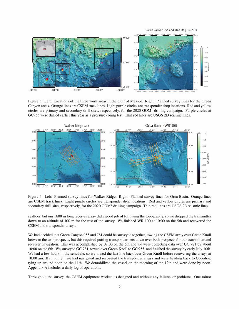
Figure 3. Left: Locations of the three work areas in the Gulf of Mexico. Right: Planned survey lines for the GreenCanyon areas. Orange lines are CSEM track lines. Light purple circles are transponder drop locations. Red and yellowcircles are primary and secondary drill sites, respectively, for the 2020 GOM2 drilling campaign. Purple circles atGC955 were drilled earlier this year as a pressure coring test. Thin red lines are USGS 2D seismic lines.

Figure 4. Left: Planned survey lines for Walker Ridge. Right: Planned survey lines for Orca Basin. Orange linesare CSEM track lines. Light purple circles are transponder drop locations. Red and yellow circles are primary andsecondary drill sites, respectively, for the 2020 GOM2 drilling campaign. Thin red lines are USGS 2D seismic lines.

seafloor, but our 1600 m long receiver array did a good job of following the topography, so we dropped the transmitterdown to an altitude of 100 m for the rest of the survey. We finished WR 100 at 10:00 on the 5th and recovered theCSEM and transponder arrays.

We had decided that Green Canyon 955 and 781 could be surveyed together, towing the CSEM array over Green Knollbetween the two prospects, but this required putting transponder nets down over both prospects for our transmitter andreceiver navigation. This was accomplished by 07:00 on the 6th and we were collecting data over GC 781 by about10:00 on the 6th. We surveyed GC 781, towed over Green Knoll to GC 955, and finished the survey by early July 10th.We had a few hours in the schedule, so we towed the last line back over Green Knoll before recovering the arrays at10:00 am. By midnight we had navigated and recovered the transponder arrays and were heading back to Cocodrie,tying up around noon on the 11th. We demobilized the vessel on the morning of the 12th and were done by noon.Appendix A includes a daily log of operations.

Throughout the survey, the CSEM equipment worked as designed and without any failures or problems. One minor

5

issue we had was that one navigation transponder was deployed disabled as a consequence of accidentally receiving adisable command during deck testing the acoustic releases of other units. Since we can navigate the CSEM transmitterusing ranges from two acoustic transponders and depth, this should not compromise our survey. Another small issue isthat one of the Vulcans leaked a little water on the first deployment, and although it did not affect the data we swappedit out with a spare instrument for subsequent deployments.

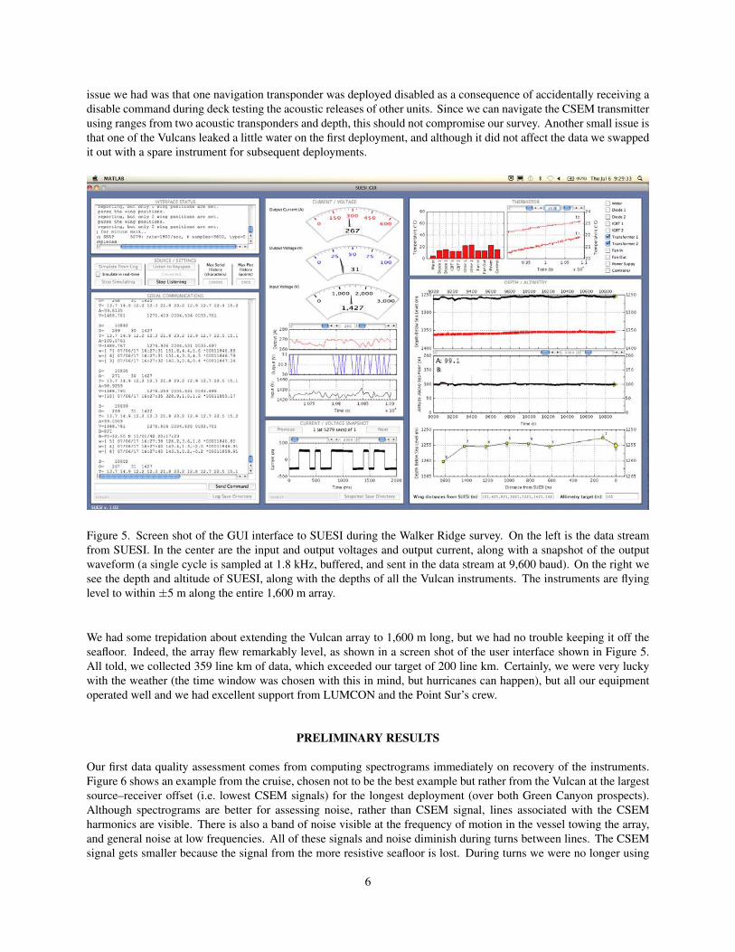
Figure 5. Screen shot of the GUI interface to SUESI during the Walker Ridge survey. On the left is the data streamfrom SUESI. In the center are the input and output voltages and output current, along with a snapshot of the outputwaveform (a single cycle is sampled at 1.8 kHz, buffered, and sent in the data stream at 9,600 baud). On the right wesee the depth and altitude of SUESI, along with the depths of all the Vulcan instruments. The instruments are flyinglevel to within ±5 m along the entire 1,600 m array.

We had some trepidation about extending the Vulcan array to 1,600 m long, but we had no trouble keeping it off theseafloor. Indeed, the array flew remarkably level, as shown in a screen shot of the user interface shown in Figure 5.All told, we collected 359 line km of data, which exceeded our target of 200 line km. Certainly, we were very luckywith the weather (the time window was chosen with this in mind, but hurricanes can happen), but all our equipmentoperated well and we had excellent support from LUMCON and the Point Sur’s crew.

PRELIMINARY RESULTS

Our first data quality assessment comes from computing spectrograms immediately on recovery of the instruments.Figure 6 shows an example from the cruise, chosen not to be the best example but rather from the Vulcan at the largestsource–receiver offset (i.e. lowest CSEM signals) for the longest deployment (over both Green Canyon prospects).Although spectrograms are better for assessing noise, rather than CSEM signal, lines associated with the CSEMharmonics are visible. There is also a band of noise visible at the frequency of motion in the vessel towing the array,and general noise at low frequencies. All of these signals and noise diminish during turns between lines. The CSEMsignal gets smaller because the signal from the more resistive seafloor is lost. During turns we were no longer using

6

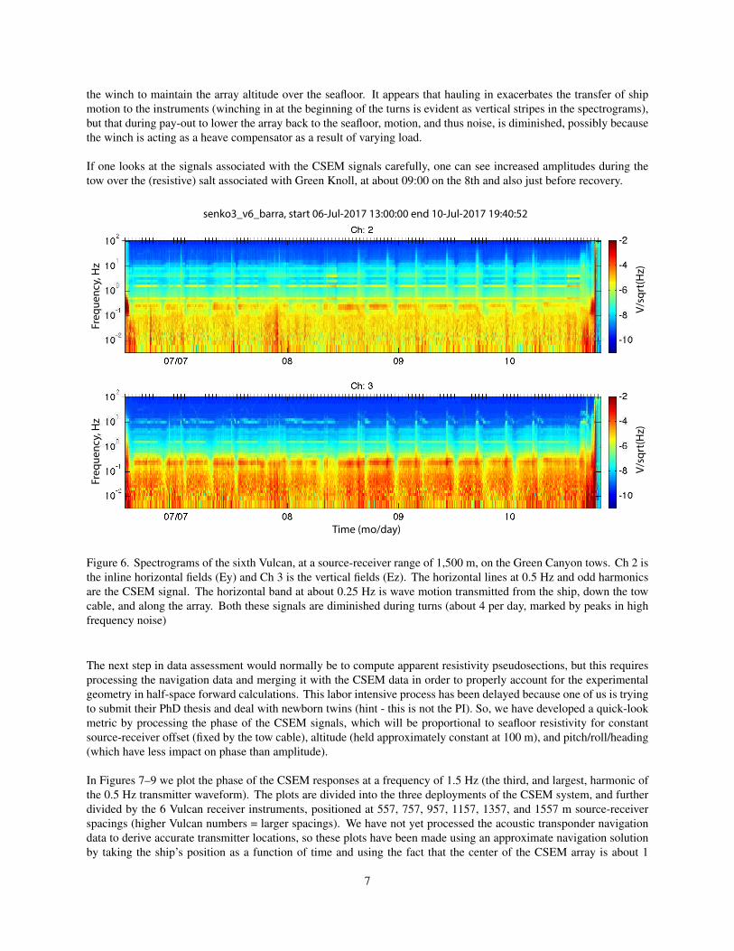
the winch to maintain the array altitude over the seafloor. It appears that hauling in exacerbates the transfer of shipmotion to the instruments (winching in at the beginning of the turns is evident as vertical stripes in the spectrograms),but that during pay-out to lower the array back to the seafloor, motion, and thus noise, is diminished, possibly becausethe winch is acting as a heave compensator as a result of varying load.

If one looks at the signals associated with the CSEM signals carefully, one can see increased amplitudes during thetow over the (resistive) salt associated with Green Knoll, at about 09:00 on the 8th and also just before recovery.

senko3_v6_barra, start 06-Jul-2017 13:00:00 end 10-Jul-2017 19:40:52

Time (mo/day)

Freq

uenc

y, H

zFr

eque

ncy,

Hz

V/sq

rt(H

z)V/

sqrt

(Hz)

Figure 6. Spectrograms of the sixth Vulcan, at a source-receiver range of 1,500 m, on the Green Canyon tows. Ch 2 isthe inline horizontal fields (Ey) and Ch 3 is the vertical fields (Ez). The horizontal lines at 0.5 Hz and odd harmonicsare the CSEM signal. The horizontal band at about 0.25 Hz is wave motion transmitted from the ship, down the towcable, and along the array. Both these signals are diminished during turns (about 4 per day, marked by peaks in highfrequency noise)

The next step in data assessment would normally be to compute apparent resistivity pseudosections, but this requiresprocessing the navigation data and merging it with the CSEM data in order to properly account for the experimentalgeometry in half-space forward calculations. This labor intensive process has been delayed because one of us is tryingto submit their PhD thesis and deal with newborn twins (hint - this is not the PI). So, we have developed a quick-lookmetric by processing the phase of the CSEM signals, which will be proportional to seafloor resistivity for constantsource-receiver offset (fixed by the tow cable), altitude (held approximately constant at 100 m), and pitch/roll/heading(which have less impact on phase than amplitude).

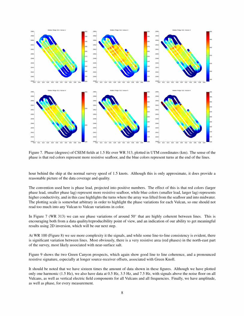
In Figures 7–9 we plot the phase of the CSEM responses at a frequency of 1.5 Hz (the third, and largest, harmonic ofthe 0.5 Hz transmitter waveform). The plots are divided into the three deployments of the CSEM system, and furtherdivided by the 6 Vulcan receiver instruments, positioned at 557, 757, 957, 1157, 1357, and 1557 m source-receiverspacings (higher Vulcan numbers = larger spacings). We have not yet processed the acoustic transponder navigationdata to derive accurate transmitter locations, so these plots have been made using an approximate navigation solutionby taking the ship’s position as a function of time and using the fact that the center of the CSEM array is about 1

7

620 622 624 626 628 630 632 634 636 638 6402938

2940

2942

2944

2946

2948

2950

2952

2954

2956

2958

2960Walker Ridge 313, Vulcan 1

250

255

260

265

270

275

280

285

290

295

300

620 622 624 626 628 630 632 634 636 638 6402938

2940

2942

2944

2946

2948

2950

2952

2954

2956

2958


200

210

220

230

240

250

260

270

280

290

300

620 622 624 626 628 630 632 634 636 638 6402938

2940

2942

2944

2946

2948

2950

2952

2954

2956

2958


180

200

220

240

260

280

300

620 622 624 626 628 630 632 634 636 638 6402938

2940

2942

2944

2946

2948

2950

2952

2954

2956

2958


150

200

250

300

620 622 624 626 628 630 632 634 636 638 6402938

2940

2942

2944

2946

2948

2950

2952

2954

2956

2958


100

120

140

160

180

200

220

240

260

280

300

620 622 624 626 628 630 632 634 636 638 6402938

2940

2942

2944

2946

2948

2950

2952

2954

2956

2958


100

120

140

160

180

200

220

240

260

280

300

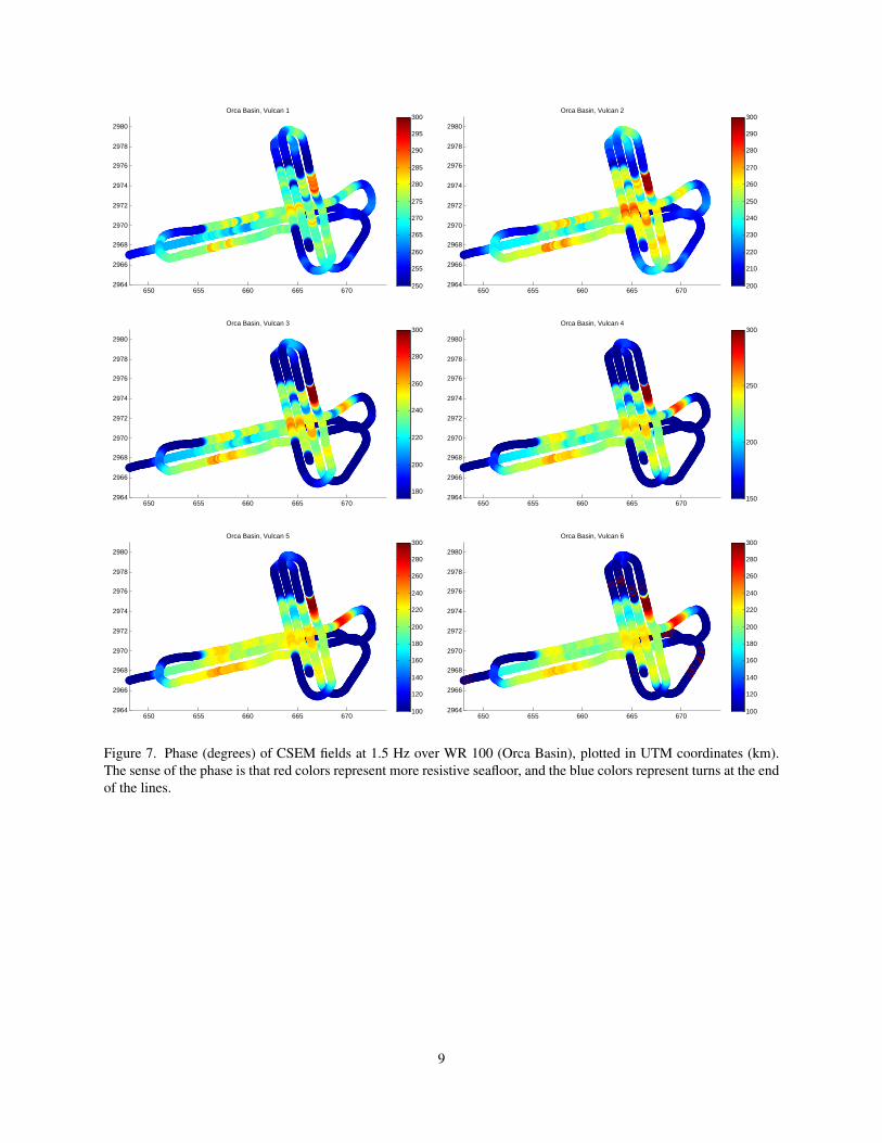
Figure 7. Phase (degrees) of CSEM fields at 1.5 Hz over WR 313, plotted in UTM coordinates (km). The sense of thephase is that red colors represent more resistive seafloor, and the blue colors represent turns at the end of the lines.

hour behind the ship at the normal survey speed of 1.5 knots. Although this is only approximate, it does provide areasonable picture of the data coverage and quality.

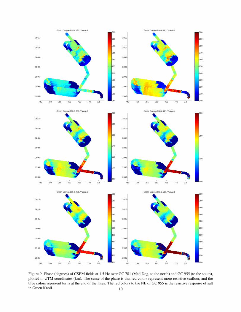
The convention used here is phase lead, projected into positive numbers. The effect of this is that red colors (largerphase lead, smaller phase lag) represent more resistive seafloor, while blue colors (smaller lead, larger lag) representshigher conductivity, and in this case highlights the turns where the array was lifted from the seafloor and into midwater.The plotting scale is somewhat arbitrary in order to highlight the phase variations for each Vulcan, so one should notread too much into any Vulcan to Vulcan variations in color.

In Figure 7 (WR 313) we can see phase variations of around 50 that are highly coherent between lines. This isencouraging both from a data quality/reproducibility point of view, and an indication of our ability to get meaningfulresults using 2D inversion, which will be our next step.

At WR 100 (Figure 8) we see more complexity it the signals, and while some line-to-line consistency is evident, thereis significant variation between lines. Most obviously, there is a very resistive area (red phases) in the north-east partof the survey, most likely associated with near-surface salt.

Figure 9 shows the two Green Canyon prospects, which again show good line to line coherence, and a pronouncedresistive signature, especially at longer source-receiver offsets, associated with Green Knoll.

It should be noted that we have sixteen times the amount of data shown in these figures. Although we have plottedonly one harmonic (1.5 Hz), we also have data at 0.5 Hz, 3.5 Hz, and 7.5 Hz, with signals above the noise floor on allVulcans, as well as vertical electric field components for all Vulcans and all frequencies. Finally, we have amplitude,as well as phase, for every measurement.

8

650 655 660 665 6702964

2966

2968

2970

2972

2974

2976

2978

2980

Orca Basin, Vulcan 1

250

255

260

265

270

275

280

285

290

295

300

650 655 660 665 6702964

2966

2968

2970

2972

2974

2976

2978

2980


200

210

220

230

240

250

260

270

280

290

300

650 655 660 665 6702964

2966

2968

2970

2972

2974

2976

2978

2980


180

200

220

240

260

280

300

650 655 660 665 6702964

2966

2968

2970

2972

2974

2976

2978

2980


150

200

250

300

650 655 660 665 6702964

2966

2968

2970

2972

2974

2976

2978

2980


100

120

140

160

180

200

220

240

260

280

300

650 655 660 665 6702964

2966

2968

2970

2972

2974

2976

2978

2980


100

120

140

160

180

200

220

240

260

280

300

Figure 7. Phase (degrees) of CSEM fields at 1.5 Hz over WR 100 (Orca Basin), plotted in UTM coordinates (km).The sense of the phase is that red colors represent more resistive seafloor, and the blue colors represent turns at the endof the lines.

9

745 750 755 760 765 770 775

2985

2990

2995

3000

3005

3010

3015

Green Canyon 955 & 781, Vulcan 1

250

255

260

265

270

275

280

285

290

295

300

745 750 755 760 765 770 775

2985

2990

2995

3000

3005

3010

3015


200

210

220

230

240

250

260

270

280

290

300

745 750 755 760 765 770 775

2985

2990

2995

3000

3005

3010

3015


180

200

220

240

260

280

300

745 750 755 760 765 770 775

2985

2990

2995

3000

3005

3010

3015


150

200

250

300

745 750 755 760 765 770 775

2985

2990

2995

3000

3005

3010

3015


100

120

140

160

180

200

220

240

260

280

300

745 750 755 760 765 770 775

2985

2990

2995

3000

3005

3010

3015


100

120

140

160

180

200

220

240

260

280

300

Figure 9. Phase (degrees) of CSEM fields at 1.5 Hz over GC 781 (Mad Dog, to the north) and GC 955 (to the south),plotted in UTM coordinates (km). The sense of the phase is that red colors represent more resistive seafloor, and theblue colors represent turns at the end of the lines. The red colors to the NE of GC 955 is the resistive response of saltin Green Knoll. 10

Appendix ADaily Log

All times are local.

28 June10:00 Arrive LUMCON and start loading.20:00 SUESI tests OK on deck.

29 June08:00 Push off.

30 June03:20 Arrive on station WR 313 and deploy transponder net.04:45 Transponder 4 in water. Transit to deployment run-in.06:00 On station.06:20 Array going in.09:10 SUESI tests OK.09:22 SUESI in water.11:35 SUESI at flying altitude.

1 JulyTowing WR 313.

2 July10:44 Crewmember accidentally pushed emergency stop. Restart SUESI.18:15 End of survey. Hauling in.20:10 SUESI on deck.22:00 Array on board. Transit to transponder recovery.23:15 Start transponder navigation and recovery.

3 July04:20 Transponders recovered, transit to WR 100.06:46 Deploy transponders.07:30 Transponder 4 in water. Transit to deployment run-in.09:00 Array going in.12:00 SUESI in water.

4 JulyTowing WR 100.

5 July10:00 End of survey Hauling in.12:30 SUESI on deck after break for lunch.14:00 Array on board.20:00 Transit to Green Canyon.

6 July01:20 Deploy transponders on GC 955.03:26 Deploy transponders on GC 781.08:20 SUESI in water GC 781.

7 July

11

Survey GC 781.

8 July

9 July

10 July10:00 Haul in for final recovery.12:00 SUESI on deck. Break for lunch.13:25 Array on board.14:05 Start transponder navigation and recovery.23:45 Transponder recovery complete. Heading to Cocodrie.

11 July13:00 Tie up and demob.

12 July11:00 Science party leaves.

12

Appendix BSUESI synchs

These are the times that SUESI’s onboard clock is synchronized to GPS time, and the second counters in SUESI’s datastream start at these times.

June 30 2017 181:15:23:00July 2 2017 183:10:51:00 (accidental trip of Elgar).July 3 2017 184:17:04:00July 6 2017 187:13:26:00

13

Appendix CVulcan array dimensions

SUESI 1AltimeterValeport 70 ft lead-in rope used on 100m long antenna on winchBenthos

Serial Communication and timing 2015 in ext. pressure case VMG-4-FS

10.0 meters15.0 meters center of near antenna copper electrode (10m of 1/2" copper tube) Tested Dec 2016:65.0 metersDIPOLE CENTER pin 1 - 6.6 Ω 110.0 meters pin 2 - 6.6 Ω115.0 meters center of long antenna copper electrode (10m of 1/2" copper tube) pin 3 - 6.6 Ω 120.0 meters End of copper on long (110m) antenna pin 4 - 6.6 Ω

transmit X.X kHz chinese fingerreceive X.X kHz VMG-4-FS 15/32" ss quick link

Optical isolation and serial communication 2012. Address=1Termination required

RS422 Serial communication 2013 Address=2Paroscientific Depth Gauge to SDL 2013 VMG-4-FS 15/32" ss quick linkCompass to SDL 2013 chinese finger

500 meters Falmat 4 conductor RS-

422 cable SN 500M-1302

Tested December 2016: pin1 - 24.0Ω pin 2 - 25.5Ω pin 3 - 25.5Ω pin 4 - 26.0Ω

8 channel data logger dipole chinese fingerch.1 E-field, X, wing, horizontal 1 meter 15/32" ss quick linkch.2 E-field, Y, stinger, horizontal 2 meter VMG-4-MPch.3 E-field, Y, fin, vertical 1 meter VMG-4-FSch.4 Accelerometer, X, wing, horizontalch.5 Accelerometer, Y, stinger, horizontalch.6 Accelerometer, Y, fin, vertical VMG-4-FS

Serial communication and timing 2015 Address=3 VMG-4-MPParoscientific Depth Gauge to SDL 2015 15/32" ss quick linkCompass to SDL 2015 chinese finger




Tested December 2016: pin1- 9.7Ω pin 2- 10.1Ω pin 3- 10.2Ω pin 4- 10.0Ω





Serial communication and timing 2015 Address=6 VMG-4-MPParoscientific Depth Gauge to SDL 2015 15/32" ss quick linkCompass to SDL 2015


8 channel data logger dipole chinese finger

ch.1 E-field, X, wing, horizontal 1 meter 15/32" ss quick link

ch.2 E-field, Y, stinger, horizontal 2 meter VMG-4-MPch.3 E-field, Y, fin, vertical 1 meter VMG-4-FSch.4 Accelerometer, X, wing, horizontalch.5 Accelerometer, Y, stinger, horizontalch.6 Accelerometer, Y, fin, vertical VMG-4-FS

Serial communication and timing 2015 Address=7 VMG-4-MP

Paroscientific Depth Gauge to SDL 2015 15/32" ss quick link

Compass to SDL 2015







Compass to SDL 2015


VMG-4-FS chinese finger15/32" ss quick link

Tritech Altimeter to SDL 2015

Serial communication 2015 Address=9Paroscientific Depth Gauge to SDL 2015Compass to SDL 2015

transmit X.X kHz 15/32" ss quick link

receive X.X kHzBurn wire release system?


15/32" ss quick link3.5 m Amsteel line to orange

drogue SN 080715/32" ss quick link

DROGUE

1222.0 meters


422 cable SN 200M-1306

1422.0

VMG-4-FS

meters

meters

Vulcan Data Logger System

(center of Y-axis dipole)

3.5 m 1/4" Amsteel Blue Pair SN 0826VMG-4-FS

2017 Gulf of Mexico DoE SUESI/Vulcan towed system arrangement

Acoustics, LBL

VMG-4-FS 3.5 m 1/4" Amsteel Blue Pair SN 1303

3.5 m 1/4" Amsteel Blue Pair SN 0825

3.5 m 1/4" Amsteel Blue Pair SN1310

VMG-4-FS VMG-4-MP

Spooled on blue InterOcean winch and updated 12-14-16, CA




VMG-4-FS



622.0

822.0 meters



meters




422 cable SN 200M-1301


422 cable SN 200M-1302


422 cable SN 200M-1305

0 meters

125 meters Falmat 4 conductor RS-422 cable (spiral

wrapped on 110m SUESI antenna )

LBL ATET 2013 Antenna Tail End Telemetry (center

of harness)

121.8 meters

VMG-4-FS VMG-4-MP

end of 10 m x 1.46"near antenna

SUESI 1

end of 100 m 1.46" antenna on 10m strain relief (110m total length)

1022.0



422 cable SN 200M-1303

1622.0 meters





422 cable SN 10M-1501

VMG-4-MP


1632.4 meters

BTET with Altimeter &

Telemetry (center of altimeter)

VMG-4-FS

Acoustics, LBLLBL CTET with SBL

acoustics (center of harness)

meters1635.2 3.24 m 1/4" Amsteel Blue Pair SN 1311

Continued on next page...

14

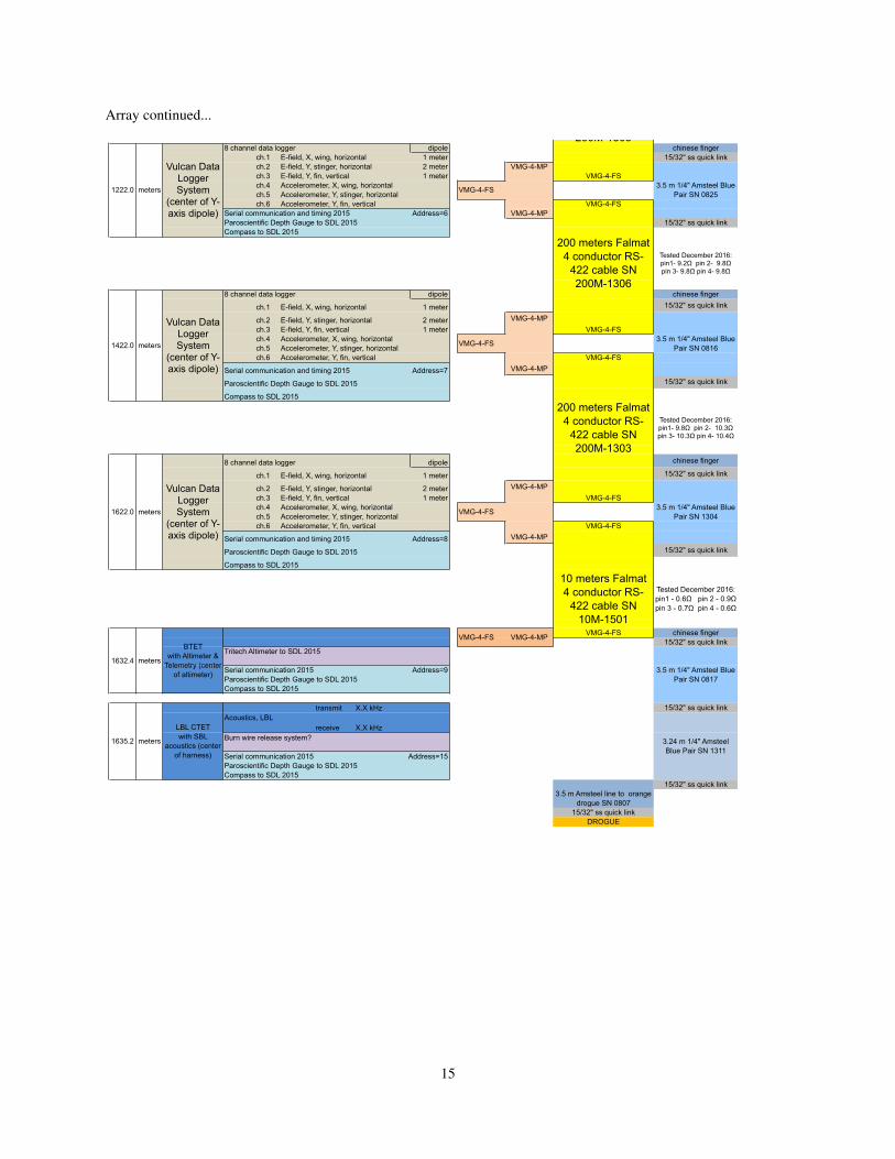
Array continued...

SUESI 1AltimeterValeport 70 ft lead-in rope used on 100m long antenna on winchBenthos

Serial Communication and timing 2015 in ext. pressure case VMG-4-FS

10.0 meters15.0 meters center of near antenna copper electrode (10m of 1/2" copper tube) Tested Dec 2016:65.0 metersDIPOLE CENTER pin 1 - 6.6 Ω 110.0 meters pin 2 - 6.6 Ω115.0 meters center of long antenna copper electrode (10m of 1/2" copper tube) pin 3 - 6.6 Ω 120.0 meters End of copper on long (110m) antenna pin 4 - 6.6 Ω

transmit X.X kHz chinese fingerreceive X.X kHz VMG-4-FS 15/32" ss quick link

Optical isolation and serial communication 2012. Address=1Termination required

RS422 Serial communication 2013 Address=2Paroscientific Depth Gauge to SDL 2013 VMG-4-FS 15/32" ss quick linkCompass to SDL 2013 chinese finger


422 cable SN 500M-1302












Serial communication and timing 2015 Address=6 VMG-4-MPParoscientific Depth Gauge to SDL 2015 15/32" ss quick linkCompass to SDL 2015







Compass to SDL 2015







Compass to SDL 2015


VMG-4-FS chinese finger15/32" ss quick link

Tritech Altimeter to SDL 2015


transmit X.X kHz 15/32" ss quick link

receive X.X kHzBurn wire release system?


15/32" ss quick link3.5 m Amsteel line to orange

drogue SN 080715/32" ss quick link

DROGUE

1222.0 meters


422 cable SN 200M-1306

1422.0

VMG-4-FS

meters

meters




2017 Gulf of Mexico DoE SUESI/Vulcan towed system arrangement

Acoustics, LBL

VMG-4-FS 3.5 m 1/4" Amsteel Blue Pair SN 1303


3.5 m 1/4" Amsteel Blue Pair SN1310

VMG-4-FS VMG-4-MP

Spooled on blue InterOcean winch and updated 12-14-16, CA




VMG-4-FS



622.0

822.0 meters



meters




422 cable SN 200M-1301


422 cable SN 200M-1302


422 cable SN 200M-1305

0 meters

125 meters Falmat 4 conductor RS-422 cable (spiral

wrapped on 110m SUESI antenna )

LBL ATET 2013 Antenna Tail End Telemetry (center

of harness)

121.8 meters

VMG-4-FS VMG-4-MP

end of 10 m x 1.46"near antenna

SUESI 1

end of 100 m 1.46" antenna on 10m strain relief (110m total length)

1022.0



422 cable SN 200M-1303

1622.0 meters





422 cable SN 10M-1501

VMG-4-MP


1632.4 meters

BTET with Altimeter &

Telemetry (center of altimeter)

VMG-4-FS

Acoustics, LBLLBL CTET with SBL

acoustics (center of harness)

meters1635.2 3.24 m 1/4" Amsteel Blue Pair SN 1311

15

Preliminary Cruise Report Marine CSEM Surveys of Green … · Preliminary Cruise Report Marine CSEM...

Documents

Transcript of Preliminary Cruise Report Marine CSEM Surveys of Green … · Preliminary Cruise Report Marine CSEM...