Preliminaries: Statistical and Causal Models

�

� �

�

1Preliminaries: Statisticaland Causal Models

1.1 Why Study Causation

The answer to the question “why study causation?” is almost as immediate as the answer to“why study statistics.” We study causation because we need to make sense of data, to guideactions and policies, and to learn from our success and failures. We need to estimate the effectof smoking on lung cancer, of education on salaries, of carbon emissions on the climate. Mostambitiously, we also need to understand how and why causes influence their effects, whichis not less valuable. For example, knowing whether malaria is transmitted by mosquitoes or“mal-air,” as many believed in the past, tells us whether we should pack mosquito nets orbreathing masks on our next trip to the swamps.

Less obvious is the answer to the question, “why study causation as a separate topic, distinctfrom the traditional statistical curriculum?” What can the concept of “causation,” consideredon its own, tell us about the world that tried-and-true statistical methods can’t?

Quite a lot, as it turns out. When approached rigorously, causation is not merely an aspect ofstatistics; it is an addition to statistics, an enrichment that allows statistics to uncover workingsof the world that traditional methods alone cannot. For example, and this might come as asurprise to many, none of the problems mentioned above can be articulated in the standardlanguage of statistics.

To understand the special role of causation in statistics, let’s examine one of the most intrigu-ing puzzles in the statistical literature, one that illustrates vividly why the traditional languageof statistics must be enriched with new ingredients in order to cope with cause–effect relation-ships, such as the ones we mentioned above.

1.2 Simpson’s Paradox

Named after Edward Simpson (born 1922), the statistician who first popularized it, the paradoxrefers to the existence of data in which a statistical association that holds for an entire popu-lation is reversed in every subpopulation. For instance, we might discover that students who

Causal Inference in Statistics: A Primer, First Edition. Judea Pearl, Madelyn Glymour, and Nicholas P. Jewell.© 2016 John Wiley & Sons, Ltd. Published 2016 by John Wiley & Sons, Ltd.Companion Website: www.wiley.com/go/Pearl/Causality

Selected preview pages from Chapter 1 (pp. 1-7 & 24-33) of J. Pearl, M. Glymour, and N.P. Jewell, Causal Inference in Statistics: A Primer, Wiley, 2016.

�

� �

�

2 Causal Inference in Statistics

smoke get higher grades, on average, than nonsmokers get. But when we take into accountthe students’ age, we might find that, in every age group, smokers get lower grades thannonsmokers get. Then, if we take into account both age and income, we might discover thatsmokers once again get higher grades than nonsmokers of the same age and income. Thereversals may continue indefinitely, switching back and forth as we consider more and moreattributes. In this context, we want to decide whether smoking causes grade increases and inwhich direction and by how much, yet it seems hopeless to obtain the answers from the data.

In the classical example used by Simpson (1951), a group of sick patients are given theoption to try a new drug. Among those who took the drug, a lower percentage recovered thanamong those who did not. However, when we partition by gender, we see that more men takingthe drug recover than do men are not taking the drug, and more women taking the drug recoverthan do women are not taking the drug! In other words, the drug appears to help men andwomen, but hurt the general population. It seems nonsensical, or even impossible—which iswhy, of course, it is considered a paradox. Some people find it hard to believe that numberscould even be combined in such a way. To make it believable, then, consider the followingexample:

Example 1.2.1 We record the recovery rates of 700 patients who were given access to thedrug. A total of 350 patients chose to take the drug and 350 patients did not. The results of thestudy are shown in Table 1.1.

The first row shows the outcome for male patients; the second row shows the outcome forfemale patients; and the third row shows the outcome for all patients, regardless of gender.In male patients, drug takers had a better recovery rate than those who went without the drug(93% vs 87%). In female patients, again, those who took the drug had a better recovery ratethan nontakers (73% vs 69%). However, in the combined population, those who did not takethe drug had a better recovery rate than those who did (83% vs 78%).

The data seem to say that if we know the patient’s gender—male or female—we can pre-scribe the drug, but if the gender is unknown we should not! Obviously, that conclusion isridiculous. If the drug helps men and women, it must help anyone; our lack of knowledge ofthe patient’s gender cannot make the drug harmful.

Given the results of this study, then, should a doctor prescribe the drug for a woman? Aman? A patient of unknown gender? Or consider a policy maker who is evaluating the drug’soverall effectiveness on the population. Should he/she use the recovery rate for the generalpopulation? Or should he/she use the recovery rates for the gendered subpopulations?

Table 1.1 Results of a study into a new drug, with gender being taken into account

Drug No drug

Men 81 out of 87 recovered (93%) 234 out of 270 recovered (87%)Women 192 out of 263 recovered (73%) 55 out of 80 recovered (69%)Combined data 273 out of 350 recovered (78%) 289 out of 350 recovered (83%)

�

� �

�

Preliminaries: Statistical and Causal Models 3

The answer is nowhere to be found in simple statistics. In order to decide whether the drugwill harm or help a patient, we first have to understand the story behind the data—the causalmechanism that led to, or generated, the results we see. For instance, suppose we knew anadditional fact: Estrogen has a negative effect on recovery, so women are less likely to recoverthan men, regardless of the drug. In addition, as we can see from the data, women are signifi-cantly more likely to take the drug than men are. So, the reason the drug appears to be harmfuloverall is that, if we select a drug user at random, that person is more likely to be a woman andhence less likely to recover than a random person who does not take the drug. Put differently,being a woman is a common cause of both drug taking and failure to recover. Therefore, toassess the effectiveness, we need to compare subjects of the same gender, thereby ensuringthat any difference in recovery rates between those who take the drug and those who do notis not ascribable to estrogen. This means we should consult the segregated data, which showsus unequivocally that the drug is helpful. This matches our intuition, which tells us that thesegregated data is “more specific,” hence more informative, than the unsegregated data.

With a few tweaks, we can see how the same reversal can occur in a continuous example.Consider a study that measures weekly exercise and cholesterol in various age groups. Whenwe plot exercise on the X-axis and cholesterol on the Y-axis and segregate by age, as inFigure 1.1, we see that there is a general trend downward in each group; the more youngpeople exercise, the lower their cholesterol is, and the same applies for middle-aged peopleand the elderly. If, however, we use the same scatter plot, but we don’t segregate by gender(as in Figure 1.2), we see a general trend upward; the more a person exercises, the higher theircholesterol is. To resolve this problem, we once again turn to the story behind the data. If weknow that older people, who are more likely to exercise (Figure 1.1), are also more likely tohave high cholesterol regardless of exercise, then the reversal is easily explained, and easilyresolved. Age is a common cause of both treatment (exercise) and outcome (cholesterol). Sowe should look at the age-segregated data in order to compare same-age people and therebyeliminate the possibility that the high exercisers in each group we examine are more likely tohave high cholesterol due to their age, and not due to exercising.

However, and this might come as a surprise to some readers, segregated data does not alwaysgive the correct answer. Suppose we looked at the same numbers from our first example of drugtaking and recovery, instead of recording participants’ gender, patients’ blood pressure were

Y

XExercise

Cholesterol

1020

3040

50Age

Figure 1.1 Results of the exercise–cholesterol study, segregated by age

�

� �

�


Y

XExercise

Cholesterol

Figure 1.2 Results of the exercise–cholesterol study, unsegregated. The data points are identical tothose of Figure 1.1, except the boundaries between the various age groups are not shown

recorded at the end of the experiment. In this case, we know that the drug affects recoveryby lowering the blood pressure of those who take it—but unfortunately, it also has a toxiceffect. At the end of our experiment, we receive the results shown in Table 1.2. (Table 1.2 isnumerically identical to Table 1.1, with the exception of the column labels, which have beenswitched.)

Now, would you recommend the drug to a patient?Once again, the answer follows from the way the data were generated. In the general pop-

ulation, the drug might improve recovery rates because of its effect on blood pressure. Butin the subpopulations—the group of people whose posttreatment BP is high and the groupwhose posttreatment BP is low—we, of course, would not see that effect; we would only seethe drug’s toxic effect.

As in the gender example, the purpose of the experiment was to gauge the overall effect oftreatment on rates of recovery. But in this example, since lowering blood pressure is one ofthe mechanisms by which treatment affects recovery, it makes no sense to separate the resultsbased on blood pressure. (If we had recorded the patients’ blood pressure before treatment,and if it were BP that had an effect on treatment, rather than the other way around, it would bea different story.) So we consult the results for the general population, we find that treatmentincreases the probability of recovery, and we decide that we should recommend treatment.Remarkably, though the numbers are the same in the gender and blood pressure examples, thecorrect result lies in the segregated data for the former and the aggregate data for the latter.

None of the information that allowed us to make a treatment decision—not the timing of themeasurements, not the fact that treatment affects blood pressure, and not the fact that blood

Table 1.2 Results of a study into a new drug, with posttreatment blood pressure taken into account

No drug Drug

Low BP 81 out of 87 recovered (93%) 234 out of 270 recovered (87%)High BP 192 out of 263 recovered (73%) 55 out of 80 recovered (69%)Combined data 273 out of 350 recovered (78%) 289 out of 350 recovered (83%)

�

� �

�


pressure affects recovery—was found in the data. In fact, as statistics textbooks have tradi-tionally (and correctly) warned students, correlation is not causation, so there is no statisticalmethod that can determine the causal story from the data alone. Consequently, there is nostatistical method that can aid in our decision.

Yet statisticians interpret data based on causal assumptions of this kind all the time. In fact,the very paradoxical nature of our initial, qualitative, gender example of Simpson’s problemis derived from our strongly held conviction that treatment cannot affect sex. If it could, therewould be no paradox, since the causal story behind the data could then easily assume the samestructure as in our blood pressure example. Trivial though the assumption “treatment does notcause sex” may seem, there is no way to test it in the data, nor is there any way to representit in the mathematics of standard statistics. There is, in fact, no way to represent any causalinformation in contingency tables (such as Tables 1.1 and 1.2), on which statistical inferenceis often based.

There are, however, extra-statistical methods that can be used to express and interpret causalassumptions. These methods and their implications are the focus of this book. With the help ofthese methods, readers will be able to mathematically describe causal scenarios of any com-plexity, and answer decision problems similar to those posed by Simpson’s paradox as swiftlyand comfortably as they can solve for X in an algebra problem. These methods will allow us toeasily distinguish each of the above three examples and move toward the appropriate statisti-cal analysis and interpretation. A calculus of causation composed of simple logical operationswill clarify the intuitions we already have about the nonexistence of a drug that cures menand women but hurts the whole population and about the futility of comparing patients withequal blood pressure. This calculus will allow us to move beyond the toy problems of Simp-son’s paradox into intricate problems, where intuition can no longer guide the analysis. Simplemathematical tools will be able to answer practical questions of policy evaluation as well asscientific questions of how and why events occur.

But we’re not quite ready to pull off such feats of derring-do just yet. In order to rigorouslyapproach our understanding of the causal story behind data, we need four things:

1. A working definition of “causation.”2. A method by which to formally articulate causal assumptions—that is, to create causal

models.3. A method by which to link the structure of a causal model to features of data.4. A method by which to draw conclusions from the combination of causal assumptions

embedded in a model and data.

The first two parts of this book are devoted to providing methods for modeling causalassumptions and linking them to data sets, so that in the third part, we can use those assump-tions and data to answer causal questions. But before we can go on, we must define causation.It may seem intuitive or simple, but a commonly agreed-upon, completely encompassing def-inition of causation has eluded statisticians and philosophers for centuries. For our purposes,the definition of causation is simple, if a little metaphorical: A variable X is a cause of a vari-able Y if Y in any way relies on X for its value. We will expand slightly upon this definitionlater, but for now, think of causation as a form of listening; X is a cause of Y if Y listens to Xand decides its value in response to what it hears.

Readers must also know some elementary concepts from probability, statistics, and graphtheory in order to understand the aforementioned causal methods. The next two sections

�

� �

�


will therefore provide the necessary definitions and examples. Readers with a basic under-standing of probability, statistics, and graph theory may skip to Section 1.5 with no loss ofunderstanding.

Study questions

Study question 1.2.1

What is wrong with the following claims?

(a) “Data show that income and marriage have a high positive correlation. Therefore, yourearnings will increase if you get married.”

(b) “Data show that as the number of fires increase, so does the number of fire fighters. There-fore, to cut down on fires, you should reduce the number of fire fighters.”

(c) “Data show that people who hurry tend to be late to their meetings. Don’t hurry, or you’llbe late.”


A baseball batter Tim has a better batting average than his teammate Frank. However, some-one notices that Frank has a better batting average than Tim against both right-handed andleft-handed pitchers. How can this happen? (Present your answer in a table.)


Determine, for each of the following causal stories, whether you should use the aggregate orthe segregated data to determine the true effect.

(a) There are two treatments used on kidney stones: Treatment A and Treatment B. Doctorsare more likely to use Treatment A on large (and therefore, more severe) stones and morelikely to use Treatment B on small stones. Should a patient who doesn’t know the size ofhis or her stone examine the general population data, or the stone size-specific data whendetermining which treatment will be more effective?

(b) There are two doctors in a small town. Each has performed 100 surgeries in his career,which are of two types: one very difficult surgery and one very easy surgery. The first doctorperforms the easy surgery much more often than the difficult surgery and the second doctorperforms the difficult surgery more often than the easy surgery. You need surgery, but youdo not know whether your case is easy or difficult. Should you consult the success rateof each doctor over all cases, or should you consult their success rates for the easy anddifficult cases separately, to maximize the chance of a successful surgery?


In an attempt to estimate the effectiveness of a new drug, a randomized experiment is con-ducted. In all, 50% of the patients are assigned to receive the new drug and 50% to receive aplacebo. A day before the actual experiment, a nurse hands out lollipops to some patients who

�

� �

�


show signs of depression, mostly among those who have been assigned to treatment the nextday (i.e., the nurse’s round happened to take her through the treatment-bound ward). Strangely,the experimental data revealed a Simpson’s reversal: Although the drug proved beneficial tothe population as a whole, drug takers were less likely to recover than nontakers, among bothlollipop receivers and lollipop nonreceivers. Assuming that lollipop sucking in itself has noeffect whatsoever on recovery, answer the following questions:

(a) Is the drug beneficial to the population as a whole or harmful?(b) Does your answer contradict our gender example, where sex-specific data was deemed

more appropriate?(c) Draw a graph (informally) that more or less captures the story. (Look ahead to Section

1.4 if you wish.)(d) How would you explain the emergence of Simpson’s reversal in this story?(e) Would your answer change if the lollipops were handed out (by the same criterion) a day

after the study?

[Hint: Use the fact that receiving a lollipop indicates a greater likelihood of being assignedto drug treatment, as well as depression, which is a symptom of risk factors that lower thelikelihood of recovery.]

1.3 Probability and Statistics

Since statistics generally concerns itself not with absolutes but with likelihoods, the languageof probability is extremely important to it. Probability is similarly important to the study of cau-sation because most causal statements are uncertain (e.g., “careless driving causes accidents,”which is true, but does not mean that a careless driver is certain to get into an accident), andprobability is the way we express uncertainty. In this book, we will use the language and lawsof probability to express our beliefs and uncertainty about the world. To aid readers without astrong background in probability, we provide here a glossary of the most important terms andconcepts they will need to know in order to understand the rest of the book.

1.3.1 Variables

A variable is any property or descriptor that can take multiple values. In a study that comparesthe health of smokers and nonsmokers, for instance, some variables might be the age of theparticipant, the gender of the participant, whether or not the participant has a family historyof cancer, and how many years the participant has been smoking. A variable can be thoughtof as a question, to which the value is the answer. For instance, “How old is this participant?”“38 years old.” Here, “age” is the variable, and “38” is its value. The probability that variable Xtakes value x is written P(X = x). This is often shortened, when context allows, to P(x). We canalso discuss the probability of multiple values at once; for instance, the probability that X = xand Y = y is written P(X = x,Y = y), or P(x, y). Note that P(X = 38) is specifically interpretedas the probability that an individual randomly selected from the population is aged 38.

A variable can be either discrete or continuous. Discrete variables (sometimes called cate-gorical variables) can take one of a finite or countably infinite set of values in any range. A vari-able describing the state of a standard light switch is discrete, because it has two values: “on”

�

� �

�


Consider for example the problem of finding the best estimate of Z given two observations,X = x and Y = y. As before, we write the regression equation

Z = 𝛼 + 𝛽YY + 𝛽XX + 𝜖

But now, to obtain three equations for 𝛼, 𝛽Y , and 𝛽X , we also multiply both sides by Y and Xand take expectations. Imposing the orthogonality conditions E[𝜖Y] = E[𝜖X] = 0 and solvingthe resulting equations gives

𝛽Y = RZY⋅X =𝜎

2X𝜎ZY − 𝜎ZX𝜎XY

𝜎2Y𝜎

2X − 𝜎

2YX

(1.27)

𝛽X = RZX⋅Y =𝜎

2Y𝜎ZX − 𝜎ZY𝜎YX

𝜎2Y𝜎

2X − 𝜎

2YX

(1.28)

Equations (1.27) and (1.28) are generic; they give the linear regression coefficients RZY⋅Xand RZX⋅Y for any three variables in terms of their variances and covariances, and as such, theyallow us to see how sensitive these slopes are to other model parameters. In practice, however,regression slopes are estimated from sampled data by efficient “least-square” algorithms, andrarely require memorization of mathematical equations. An exception is the task of predictingwhether any of these slopes is zero, prior to obtaining any data. Such predictions are impor-tant when we contemplate choosing a set of regressors for one purpose or another, and as weshall see in Section 3.8, this task will be handled quite efficiently through the use of causalgraphs.


(a) Prove Eq. (1.22) using the orthogonality principle. [Hint: Follow the treatment ofEq. (1.26).]

(b) Find all partial regression coefficients

RYX⋅Z ,RXY⋅Z ,RYZ⋅X ,RZY⋅X ,RXZ⋅Y , and RZX⋅Y

for the craps game described in Study question 1.3.7. [Hint: Apply Eq. (1.27) and usethe variances and covariances computed for part (a) of this question.]

1.4 Graphs

We learned from Simpson’s Paradox that certain decisions cannot be made on the basis ofdata alone, but instead depend on the story behind the data. In this section, we layout a math-ematical language, graph theory, in which these stories can be conveyed. Graph theory is notgenerally taught in high school mathematics, but it provides a useful mathematical languagethat allows us to address problems of causality with simple operations similar to those used tosolve arithmetic problems.

Although the word graph is used colloquially to refer to a whole range of visual aids—moreor less interchangeably with the word chart—in mathematics, a graph is a formally defined

�

� �

�


object. A mathematical graph is a collection of vertices (or, as we will call them, nodes) andedges. The nodes in a graph are connected (or not) by the edges. Figure 1.5 illustrates a simplegraph. X,Y , and Z (the dots) are nodes, and A and B (the lines) are edges.

X Y Z

BA

Figure 1.5 An undirected graph in which nodes X and Y are adjacent and nodes Y and Z are adjacentbut not X and Z

Two nodes are adjacent if there is an edge between them. In Figure 1.5, X and Y are adjacent,and Y and Z are adjacent. A graph is said to be a complete graph if there is an edge betweenevery pair of nodes in the graph.

A path between two nodes X and Y is a sequence of nodes beginning with X and endingwith Y , in which each node is connected to the next by an edge. For instance, in Figure 1.5,there is a path from X to Z, because X is connected to Y , and Y is connected to Z.

Edges in a graph can be directed or undirected. Both of the edges in Figure 1.5 areundirected, because they have no designated “in” and “out” ends. A directed edge, on theother hand, goes out of one node and into another, with the direction indicated by an arrowhead. A graph in which all of the edges are directed is a directed graph. Figure 1.6 illustratesa directed graph. In Figure 1.6, A is a directed edge from X to Y and B is a directed edge fromY to Z.

X Y Z

BA

Figure 1.6 A directed graph in which node A is a parent of B and B is a parent of C

The node that a directed edge starts from is called the parent of the node that the edge goesinto; conversely, the node that the edge goes into is the child of the node it comes from. InFigure 1.6, X is the parent of Y , and Y is the parent of Z; accordingly, Y is the child of X,and Z is the child of Y . A path between two nodes is a directed path if it can be traced alongthe arrows, that is, if no node on the path has two edges on the path directed into it, or twoedges directed out of it. If two nodes are connected by a directed path, then the first node is theancestor of every node on the path, and every node on the path is the descendant of the firstnode. (Think of this as an analogy to parent nodes and child nodes: parents are the ancestors oftheir children, and of their children’s children, and of their children’s children’s children, etc.)For instance, in Figure 1.6, X is the ancestor of both Y and Z, and both Y and Z are descendantsof X.

When a directed path exists from a node to itself, the path (and graph) is called cyclic. Adirected graph with no cycles is acyclic. For example, in Figure 1.7(a) the graph is acyclic;however, the graph in Figure 1.7(b) is cyclic. Note that in (1) there is no directed path fromany node to itself, whereas in (2) there are directed paths from X back to X, for example.

�

� �

�


(a) (b)

X

ZY

X

ZY

Figure 1.7 (a) Showing acyclic graph and (b) cyclic graph

Study questions


Consider the graph shown in Figure 1.8:

X Y Z

T

W

Figure 1.8 A directed graph used in Study question 1.4.1

(a) Name all of the parents of Z.(b) Name all the ancestors of Z.(c) Name all the children of W.(d) Name all the descendants of W.(e) Draw all (simple) paths between X and T (i.e., no node should appear more than once).(f) Draw all the directed paths between X and T.

1.5 Structural Causal Models

1.5.1 Modeling Causal Assumptions

In order to deal rigorously with questions of causality, we must have a way of formally settingdown our assumptions about the causal story behind a data set. To do so, we introduce theconcept of the structural causal model, or SCM, which is a way of describing the relevantfeatures of the world and how they interact with each other. Specifically, a structural causalmodel describes how nature assigns values to variables of interest.

Formally, a structural causal model consists of two sets of variables U and V , and a set offunctions f that assigns each variable in V a value based on the values of the other variablesin the model. Here, as promised, we expand on our definition of causation: A variable X is adirect cause of a variable Y if X appears in the function that assigns Y’s value. X is a cause ofY if it is a direct cause of Y , or of any cause of Y .

�

� �

�


The variables in U are called exogenous variables, meaning, roughly, that they are external tothe model; we choose, for whatever reason, not to explain how they are caused. The variablesin V are endogenous. Every endogenous variable in a model is a descendant of at least oneexogenous variable. Exogenous variables cannot be descendants of any other variables, and inparticular, cannot be a descendant of an endogenous variable; they have no ancestors and arerepresented as root nodes in graphs. If we know the value of every exogenous variable, thenusing the functions in f , we can determine with perfect certainty the value of every endogenousvariable.

For example, suppose we are interested in studying the causal relationships between a treat-ment X and lung function Y for individuals who suffer from asthma. We might assume that Yalso depends on, or is “caused by,” air pollution levels as captured by a variable Z. In this case,we would refer to X and Y as endogenous and Z as exogenous. This is because we assumethat air pollution is an external factor, that is, it cannot be caused by an individual’s selectedtreatment or their lung function.

Every SCM is associated with a graphical causal model, referred to informally as a “graph-ical model” or simply “graph.” Graphical models consist of a set of nodes representing thevariables in U and V , and a set of edges between the nodes representing the functions in f . Thegraphical model G for an SCM M contains one node for each variable in M. If, in M, the func-tion fX for a variable X contains within it the variable Y (i.e., if X depends on Y for its value),then, in G, there will be a directed edge from Y to X. We will deal primarily with SCMs forwhich the graphical models are directed acyclic graphs (DAGs). Because of the relationshipbetween SCMs and graphical models, we can give a graphical definition of causation: If, in agraphical model, a variable X is the child of another variable Y , then Y is a direct cause of X;if X is a descendant of Y , then Y is a potential cause of X (there are rare intransitive cases inwhich Y will not be a cause of X, which we will discuss in Part Two).

In this way, causal models and graphs encode causal assumptions. For instance, considerthe following simple SCM:

SCM 1.5.1 (Salary Based on Education and Experience)

U = {X,Y}, V = {Z}, F = {fZ}

fZ ∶ Z = 2X + 3Y

This model represents the salary (Z) that an employer pays an individual with X years ofschooling and Y years in the profession. X and Y both appear in fZ , so X and Y are both directcauses of Z. If X and Y had any ancestors, those ancestors would be potential causes of Z.

The graphical model associated with SCM 1.5.1 is illustrated in Figure 1.9.

Z

X Y

Figure 1.9 The graphical model of SCM 1.5.1, with X indicating years of schooling, Y indicating yearsof employment, and Z indicating salary

�

� �

�


Because there are edges connecting Z to X and Y , we can conclude just by looking at thegraphical model that there is some function fZ in the model that assigns Z a value based on Xand Y , and therefore that X and Y are causes of Z. However, without the fuller specification ofan SCM, we can’t tell from the graph what the function is that defines Z—or, in other words,how X and Y cause Z.

If graphical models contain less information than SCMs, why do we use them at all? Thereare several reasons. First, usually the knowledge that we have about causal relationships is notquantitative, as demanded by an SCM, but qualitative, as represented in a graphical model.We know off-hand that sex is a cause of height and that height is a cause of performance inbasketball, but we would hesitate to give numerical values to these relationships. We could,instead of drawing a graph, simply create a partially specified version of the SCM:

SCM 1.5.2 (Basketball Performance Based on Height and Sex)

V = {Height, Sex, Performance}, U = {U1,U2,U3}, F = {f 1, f 2}

Sex = U1

Height = f1(Sex, U2)

Performance = f2(Height, Sex, U3)

Here, U = {U1,U2,U3} represents unmeasured factors that we do not care to name, but thataffect the variables in V that we can measure. The U factors are sometimes called “error terms”or “omitted factors.” These represent additional unknown and/or random exogenous causes ofwhat we observe.

But graphical models provide a more intuitive understanding of causality than do such par-tially specified SCMs. Consider the SCM and its associated graphical model introduced above;while the SCM and its graphical model contain the same information, that is, that X causesZ and Y causes Z, that information is more quickly and easily ascertained by looking at thegraphical model.

Study questions


Suppose we have the following SCM. Assume all exogenous variables are independent andthat the expected value of each is 0.

SCM 1.5.3

V = {X,Y ,Z}, U = {UX ,UY ,UZ}, F = {fX , fY , fZ}

fX ∶ X = uX

fY ∶ Y = X3+ UY

fZ ∶ Z = Y16

+ UZ

�

� �

�


(a) Draw the graph that complies with the model.(b) Determine the best guess of the value (expected value) of Z, given that we observe Y = 3.(c) Determine the best guess of the value of Z, given that we observe X = 3.(d) Determine the best guess of the value of Z, given that we observe X = 1 and Y = 3.(e) Assume that all exogenous variables are normally distributed with zero means and unit

variance, that is, 𝜎 = 1.

(i) Determine the best guess of X, given that we observed Y = 2.(ii) (Advanced) Determine the best guess of Y, given that we observed X = 1 and Z = 3.

[Hint: You may wish to use the technique of multiple regression, together with thefact that, for every three normally distributed variables, say X, Y, and Z, we haveE[Y|X = x,Z = z] = RYX⋅Zx + RYZ⋅Xz.]

(f) Determine the best guess of the value of Z, given that we know X = 3.

1.5.2 Product Decomposition

Another advantage of graphical models is that they allow us to express joint distributions veryefficiently. So far, we have presented joint distributions in two ways. First, we have used tables,in which we assigned a probability to every possible combination of values. This is intuitivelyeasy to parse, but in models with many variables, it can take up a prohibitive amount of space;10 binary variables would require a table with 1024 rows!

Second, in a fully specified SCM, we can represent the joint distributions of n variableswith greater efficiency: We need only to specify the n functions that govern the relationshipsbetween the variables, and then from the probabilities of the error terms, we can discover allthe probabilities that govern the joint distribution. But we are not always in a position to fullyspecify a model; we may know that one variable is a cause of another but not the form of theequation relating them, or we may not know the distributions of the error terms. Even if weknow these objects, writing them down may be easier said than done, especially, when thevariables are discrete and the functions do not have familiar algebraic expressions.

Fortunately, we can use graphical models to help overcome both of these barriers throughthe following rule.

Rule of product decomposition

For any model whose graph is acyclic, the joint distribution of the variables in the model isgiven by the product of the conditional distributions P(child|parents) over all the “families” inthe graph. Formally, we write this rule as

P(x1, x2, … , xn) =∏

i

P(xi|pai) (1.29)

where pai stands for the values of the parents of variable Xi, and the product∏

i runs over alli, from 1 to n. The relationship (1.29) follows from certain universally true independenciesamong the variables, which will be discussed in the next chapter in more detail.

For example, in a simple chain graph X → Y → Z, we can write directly:

P(X = x,Y = y,Z = z) = P(X = x)P(Y = y|X = x)P(Z = z|Y = y)

�

� �

�


This knowledge allows us to save an enormous amount of space when laying out a jointdistribution. We need not create a probability table that lists a value for every possible triple(x, y, z). It will suffice to create three much smaller tables for X, (Y|X), and (Z|Y), and multiplythe values as necessary.

To estimate the joint distribution from a data set generated by the above model, we neednot count the frequency of every triple; we can instead count the frequencies of each x, (y|x),and (z|y) and multiply. This saves us a great deal of processing time in large models. Italso increases substantially the accuracy of frequency counting. Thus, the assumptionsunderlying the graph allow us to exchange a “high-dimensional” estimation problem for afew “low-dimensional” probability distribution challenges. The graph therefore simplifies anestimation problem and, simultaneously, provides more precise estimators. If we do not knowthe graphical structure of an SCM, estimation becomes impossible with large number ofvariables and small, or moderately sized, data sets—the so-called “curse of dimensionality.”

Graphical models let us do all of this without always needing to know the functions relatingthe variables, their parameters, or the distributions of their error terms.

Here’s an evocative, if unrigorous, demonstration of the time and space saved by thisstrategy: Consider the chain X → Y → Z → W, where X stands for clouds/no clouds, Ystands for rain/no rain, Z stands for wet pavement/dry pavement, and W stands for slipperypavement/unslippery pavement.

Using your own judgment, based on your experience of the world, how plausible is it thatP(clouds, no-rain, dry pavement, slippery pavement) = 0.23?

This is quite a difficult question to answer straight out. But using the product rule, we canbreak it into pieces:

P(clouds)P(no rain|clouds)P(dry pavement|no rain)P(slippery pavement|dry pavement)

Our general sense of the world tells us that P(clouds) should be relatively high, perhaps0.5 (lower, of course, for those of us living in the strange, weatherless city of Los Angeles).Similarly, P(no rain|clouds) is fairly high—say, 0.75. And P(dry pavement|no rain) wouldbe higher still, perhaps 0.9. But the P(slippery pavement|dry pavement) should be quite low,somewhere in the range of 0.05. So putting it all together, we come to a ballpark estimate of0.5 × 0.75 × 0.9 × 0.05 = 0.0169.

We will use this product rule often in this book in cases when we need to reason with numer-ical probabilities, but wish to avoid writing out large probability tables.

The importance of the product decomposition rule can be particularly appreciated whenwe deal with estimation. In fact, much of the role of statistics focuses on effective samplingdesigns, and estimation strategies, that allow us to exploit an appropriate data set to estimateprobabilities as precisely as we might need. Consider again the problem of estimating theprobability P(X,Y ,Z,W) for the chain X → Y → Z → W. This time, however, we attempt toestimate the probability from data, rather than our own judgment. The number of (x, y, z,w)combinations that need to be assigned probabilities is 16 − 1 = 15. Assume that we have 45random observations, each consisting of a vector (x, y, z,w). On the average, each (x, y, z,w)cell would receive about three samples; some will receive one or two samples, and someremain empty. It is very unlikely that we would obtain a sufficient number of samples in eachcell to assess the proportion in the population at large (i.e., when the sample size goes toinfinity).

�

� �

�


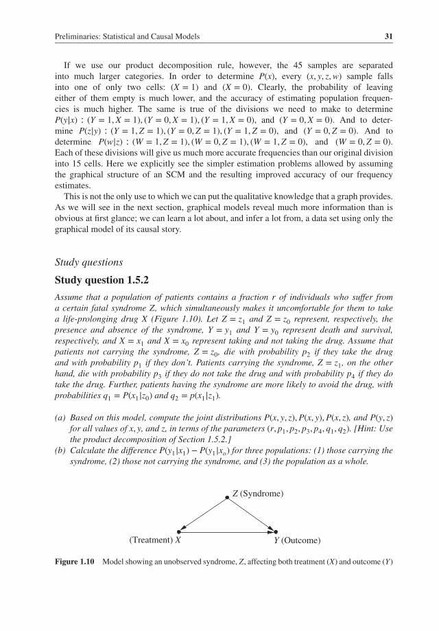
If we use our product decomposition rule, however, the 45 samples are separatedinto much larger categories. In order to determine P(x), every (x, y, z,w) sample fallsinto one of only two cells: (X = 1) and (X = 0). Clearly, the probability of leavingeither of them empty is much lower, and the accuracy of estimating population frequen-cies is much higher. The same is true of the divisions we need to make to determineP(y|x) ∶ (Y = 1,X = 1), (Y = 0,X = 1), (Y = 1,X = 0), and (Y = 0,X = 0). And to deter-mine P(z|y) ∶ (Y = 1,Z = 1), (Y = 0,Z = 1), (Y = 1,Z = 0), and (Y = 0,Z = 0). And todetermine P(w|z) ∶ (W = 1,Z = 1), (W = 0,Z = 1), (W = 1,Z = 0), and (W = 0,Z = 0).Each of these divisions will give us much more accurate frequencies than our original divisioninto 15 cells. Here we explicitly see the simpler estimation problems allowed by assumingthe graphical structure of an SCM and the resulting improved accuracy of our frequencyestimates.

This is not the only use to which we can put the qualitative knowledge that a graph provides.As we will see in the next section, graphical models reveal much more information than isobvious at first glance; we can learn a lot about, and infer a lot from, a data set using only thegraphical model of its causal story.

Study questions


Assume that a population of patients contains a fraction r of individuals who suffer froma certain fatal syndrome Z, which simultaneously makes it uncomfortable for them to takea life-prolonging drug X (Figure 1.10). Let Z = z1 and Z = z0 represent, respectively, thepresence and absence of the syndrome, Y = y1 and Y = y0 represent death and survival,respectively, and X = x1 and X = x0 represent taking and not taking the drug. Assume thatpatients not carrying the syndrome, Z = z0, die with probability p2 if they take the drugand with probability p1 if they don’t. Patients carrying the syndrome, Z = z1, on the otherhand, die with probability p3 if they do not take the drug and with probability p4 if they dotake the drug. Further, patients having the syndrome are more likely to avoid the drug, withprobabilities q1 = P(x1|z0) and q2 = p(x1|z1).

(a) Based on this model, compute the joint distributions P(x, y, z),P(x, y),P(x, z), and P(y, z)for all values of x, y, and z, in terms of the parameters (r, p1, p2, p3, p4, q1, q2). [Hint: Usethe product decomposition of Section 1.5.2.]

(b) Calculate the difference P(y1|x1) − P(y1|xo) for three populations: (1) those carrying thesyndrome, (2) those not carrying the syndrome, and (3) the population as a whole.

Y (Outcome) (Treatment) X

Z (Syndrome)

Figure 1.10 Model showing an unobserved syndrome, Z, affecting both treatment (X) and outcome (Y)

�

� �

�


(c) Using your results for (b), find a combination of parameters that exhibits Simpson’sreversal.


Consider a graph X1 → X2 → X3 → X4 of binary random variables, and assume that the con-ditional probabilities between any two consecutive variables are given by

P(Xi = 1|Xi−1 = 1) = p

P(Xi = 1|Xi−1 = 0) = q

P(X1 = 1) = p0

Compute the following probabilities

P(X1 = 1,X2 = 0,X3 = 1,X4 = 0)

P(X4 = 1|X1 = 1)

P(X1 = 1|X4 = 1)

P(X3 = 1|X1 = 0,X4 = 1)


Define the structural model that corresponds to the Monty Hall problem, and use it to describethe joint distribution of all variables.

Bibliographical Notes for Chapter 1

An extensive account of the history of Simpson’s paradoxis given in Pearl (2009, pp. 174–182),including many attempts by statisticians to resolve it without invoking causation. A morerecent account, geared for statistics instructors is given in (Pearl 2014c). Among the manytexts that provide basic introductions to probability theory, Lindley (2014) and Pearl (1988,Chapters 1 and 2) are the closest in spirit to the Bayesian perspective used in Chapter 1. Thetextbooks by Selvin (2004) and Moore et al. (2014) provide excellent introductions to clas-sical methods ofstatistics, including parameter estimation, hypothesis testing and regressionanalysis.

The Monty Hall problem, discussed in Section 1.3, appears in many introductory bookson probability theory (e.g., Grinstead and Snell 1998, p. 136; Lindley 2014, p. 201) andis mathematically equivalent to the “Three Prisoners Dilemma” discussed in (Pearl 1988,pp. 58–62). Friendly introductions to graphical models are given in Elwert (2013), Glymourand Greenland (2008), and the more advanced texts of Pearl (1988, Chapter 3), Lauritzen(1996) and Koller and Friedman (2009). The product decomposition rule of Section 1.5.2was used in Howard and Matheson (1981) and Kiiveri et al. (1984) and became the semantic

�

� �

�


basis of Bayesian Networks (Pearl 1985)—directed acyclic graphs that represent probabilisticknowledge, not necessarily causal. For inference and applications of Bayesian networks, seeDarwiche (2009) and Fenton and Neil (2013), and Conrady and Jouffe (2015). The validityof the product decomposition rule for structural causal models was shown in Pearl and Verma(1991).

Preliminaries: Statistical and Causal Models

Documents

Transcript of Preliminaries: Statistical and Causal Models