PREFERREDANDALTERNATIVE … Typical Hot-Mix Asphalt Plant Emission Control Techniques ... The...
70
VOLUME VOLUME II: II: CHAPTER CHAPTER 3 PREFERRED AND ALTERNATIVE METHODS FOR ESTIMATING AIR EMISSIONS FROM HOT-MIX ASPHALT PLANTS Final Final Report Report July July 1996 1996 Prepared by: Eastern Research Group, Inc. Post Office Box 2010 Morrisville, North Carolina 27560 Prepared for: Point Sources Committee Emission Inventory Improvement Program
Transcript of PREFERREDANDALTERNATIVE … Typical Hot-Mix Asphalt Plant Emission Control Techniques ... The...

VOLUMEVOLUME II:II: CHAPTERCHAPTER 33
PREFERRED AND ALTERNATIVEMETHODS FOR ESTIMATING AIREMISSIONS FROM HOT-MIXASPHALT PLANTS
FinalFina l Repor tReport
Jul yJul y 19961996
Prepared by:Eastern Research Group, Inc.Post Office Box 2010Morrisville, North Carolina 27560
Prepared for:Point Sources CommitteeEmission Inventory Improvement Program

DISCLAIMER
As the Environmental Protection Agency has indicated in Emission Inventory ImprovementProgram (EIIP) documents, the choice of methods to be used to estimate emissions depends onhow the estimates will be used and the degree of accuracy required. Methods using site-specificdata are preferred over other methods. These documents are non-binding guidance and not rules. EPA, the States, and others retain the discretion to employ or to require other approaches thatmeet the requirements of the applicable statutory or regulatory requirements in individualcircumstances.

ACKNOWLEDGEMENT
This document was prepared by Robert Harrison of Radian International LLC and TheresaKemmer Moody of Eastern Research Group, Inc. for the Point Sources Committee of theEmission Inventory Improvement Program and for Dennis Beauregard of the Emission Factorand Inventory Group, U.S. Environmental Protection Agency. Members of the Point SourcesCommittee contributing to the preparation of this document are:
Dennis Beauregard, Co-Chair, Emission Factor and Inventory Group, U.S. Environmental Protection AgencyBill Gill, Co-Chair, Texas Natural Resource Conservation CommissionJim Southerland, North Carolina Department of Environment, Health and Natural ResourcesDenise Alston-Guiden, Galsen CorporationBob Betterton, South Carolina Department of Health and Environmental ControlAlice Fredlund, Louisiana Department of Environmental QualityKarla Smith Hardison, Texas Natural Resource Conservation CommissionGary Helm, Air Quality Management, Inc.Paul Kim, Minnesota Pollution Control AgencyToch Mangat, Bay Area Air Quality Management DistrictRalph Patterson, Wisconsin Department of Natural Resources
EIIP Volume II iii

CHAPTER 3-HOT MIX ASPHALT PLANTS Final 7/26/96
This page is intentionally left blank.
EIIP Volume IIiv

CONTENTSSection Page
1 Introduction . . . . . . . . . . . . . . . . . . . . . . . . . . . . . . . . . . . . . . . . . . . . . . .3.1-1
2 General Source Category Description. . . . . . . . . . . . . . . . . . . . . . . . . . . . . .3.2-1
2.1 Process Description. . . . . . . . . . . . . . . . . . . . . . . . . . . . . . . . . . . . .3.2-12.1.1 Batch Mixing Process. . . . . . . . . . . . . . . . . . . . . . . . . . . . . . .3.2-22.1.2 Parallel Flow Drum Mixing Process. . . . . . . . . . . . . . . . . . . . .3.2-22.1.3 Counterflow Drum Mixing Process. . . . . . . . . . . . . . . . . . . . . .3.2-3
2.2 Emission Sources. . . . . . . . . . . . . . . . . . . . . . . . . . . . . . . . . . . . . .3.2-32.2.1 Material Handling (Fugitive Emissions). . . . . . . . . . . . . . . . . . 3.2-32.2.2 Generators. . . . . . . . . . . . . . . . . . . . . . . . . . . . . . . . . . . . . . .3.2-42.2.3 Storage Tanks. . . . . . . . . . . . . . . . . . . . . . . . . . . . . . . . . . . .3.2-42.2.4 Process Emissions. . . . . . . . . . . . . . . . . . . . . . . . . . . . . . . . .3.2-4
2.3 Process Design and Operating Factors Influencing Emissions. . . . . . . . 3.2-6
2.4 Control Techniques. . . . . . . . . . . . . . . . . . . . . . . . . . . . . . . . . . . . .3.2-82.4.1 Process and Process Fugitive Particulate Control
(Including Metals) . . . . . . . . . . . . . . . . . . . . . . . . . . . . . . . . .3.2-82.4.2 Fugitive Particulate Emissions Control. . . . . . . . . . . . . . . . . . 3.2-112.4.3 VOC (Including HAP) Control . . . . . . . . . . . . . . . . . . . . . . .3.2-112.4.4 Sulfur Oxides Control. . . . . . . . . . . . . . . . . . . . . . . . . . . . . .3.2-122.4.5 Nitrogen Oxides Control. . . . . . . . . . . . . . . . . . . . . . . . . . . .3.2-12
3 Overview of Available Methods. . . . . . . . . . . . . . . . . . . . . . . . . . . . . . . . .3.3-1
3.1 Description of Emission Estimation Methodologies. . . . . . . . . . . . . . . 3.3-13.1.1 Stack Sampling. . . . . . . . . . . . . . . . . . . . . . . . . . . . . . . . . . .3.3-13.1.2 Emission Factors. . . . . . . . . . . . . . . . . . . . . . . . . . . . . . . . . .3.3-23.1.3 Fuel Analysis. . . . . . . . . . . . . . . . . . . . . . . . . . . . . . . . . . . . .3.3-23.1.4 Continuous Emission Monitoring System (CEMS) and
Predictive Emission Monitoring (PEM). . . . . . . . . . . . . . . . . . . 3.3-2
3.2 Comparison of Available Emission Estimation Methodologies. . . . . . . 3.3-33.2.1 Stack Sampling. . . . . . . . . . . . . . . . . . . . . . . . . . . . . . . . . . .3.3-33.2.2 Emission Factors. . . . . . . . . . . . . . . . . . . . . . . . . . . . . . . . . .3.3-33.2.3 Fuel Analysis. . . . . . . . . . . . . . . . . . . . . . . . . . . . . . . . . . . . .3.3-33.2.4 CEMS and PEM. . . . . . . . . . . . . . . . . . . . . . . . . . . . . . . . . .3.3-6
EIIP Volume II v

CONTENTS (CONTINUED)Section Page
4 Preferred Methods for Estimating Emissions. . . . . . . . . . . . . . . . . . . . . . . . .3.4-1
4.1 Emission Calculations Using Stack Sampling Data. . . . . . . . . . . . . . . 3.4-14.2 Emission Factor Calculations. . . . . . . . . . . . . . . . . . . . . . . . . . . . . .3.4-54.3 Emission Calculations Using Fuel Analysis Data. . . . . . . . . . . . . . . . . 3.4-6
5 Alternative Methods for Estimating Emissions. . . . . . . . . . . . . . . . . . . . . . .3.5-1
5.1 Emission Calculations Using CEMS Data. . . . . . . . . . . . . . . . . . . . . .3.5-15.2 Predictive Emission Monitoring. . . . . . . . . . . . . . . . . . . . . . . . . . . .3.5-4
6 Quality Assurance/Quality Control. . . . . . . . . . . . . . . . . . . . . . . . . . . . . . . .3.6-1
6.1 Considerations for Using Stack Test and CEMS Data. . . . . . . . . . . . . 3.6-16.2 Considerations for Using Emission Factors. . . . . . . . . . . . . . . . . . . . .3.6-46.3 Data Attribute Rating System (DARS) Scores. . . . . . . . . . . . . . . . . . . 3.6-4
7 Data Coding Procedures. . . . . . . . . . . . . . . . . . . . . . . . . . . . . . . . . . . . . . .3.7-1
8 References. . . . . . . . . . . . . . . . . . . . . . . . . . . . . . . . . . . . . . . . . . . . . . . .3.8-1
EIIP Volume IIvi
FIGURE AND TABLESFigure Page
3.6-1 Example Emission Inventory Development Checklist for Asphalt Plants. . . . . . . 6-2
Tables Page
3.2-1 Typical Hot-Mix Asphalt Plant Emission Control Techniques. . . . . . . . . . . . . 3.2-9
3.3-1 Summary of Preferred Emission EstimationMethods for Hot-Mix Asphalt Plants. . . . . . . . . . . . . . . . . . . . . . . . . . . . . .3.3-4
3.4-1 List of Variables and Symbols. . . . . . . . . . . . . . . . . . . . . . . . . . . . . . . . . .3.4-2
3.4-2 Test Results - Method 5. . . . . . . . . . . . . . . . . . . . . . . . . . . . . . . . . . . . . . .3.4-4
3.5-1 Example CEM Output for a Parallel Flow Drum MixerFiring Waste Fuel Oil . . . . . . . . . . . . . . . . . . . . . . . . . . . . . . . . . . . . . . . .3.5-2
3.5-2 Predictive Emission Monitoring Analysis. . . . . . . . . . . . . . . . . . . . . . . . . . .3.5-6
3.6-1 DARS Scores: CEMS/PEM Data. . . . . . . . . . . . . . . . . . . . . . . . . . . . . . . .3.6-6
3.6-2 DARS Scores: Stack Sample Data. . . . . . . . . . . . . . . . . . . . . . . . . . . . . . .3.6-7
3.6-3 DARS Scores: Source-specific Emission Factor. . . . . . . . . . . . . . . . . . . . . .3.6-8
3.6-4 DARS Scores:AP-42Emission Factor . . . . . . . . . . . . . . . . . . . . . . . . . . . .3.6-9
3.7-1 Source Classification Codes for Asphalt Concrete Production. . . . . . . . . . . . . 3.7-3
3.7-2 AIRS Control Device Codes. . . . . . . . . . . . . . . . . . . . . . . . . . . . . . . . . . . .3.7-4
EIIP Volume II vii

CHAPTER 3-HOT MIX ASPHALT PLANTS Draft 3/13/96
This page is intentionally left blank.
EIIP Volume IIviii
1
INTRODUCTIONThe purposes of the preferred methods guidelines are to describe emission estimationtechniques for stationary point sources in a clear and unambiguous manner and to provideconcise example calculations to aid in the preparation of emission inventories. Whileemissions estimates are not provided, this information may be used to select an emissionestimation technique best suited to a particular application. This chapter describes theprocedures and recommends approaches for estimating emissions from hot-mix asphalt(HMA) plants.
Section 2 of this chapter contains a general description of the HMA plant source category,common emission sources, and an overview of the available control technologies used atHMA plants. Section 3 of this chapter provides an overview of available emissionestimation methods.
Section 4 presents the preferred methods for estimating emissions from HMA plants, whileSection 5 presents the alternative emission estimation techniques. It should be noted that theuse of site-specific emission data is preferred over the use of industry-averaged data such asAP-42emission factors (EPA, 1995a). Depending upon available resources, site-specific datamay not be cost effective to obtain. However, this site-specific data may be a requirement ofthe state implementation plan (SIP) and may preclude the use of other data. Qualityassurance and control procedures are described in Section 6. Coding procedures used fordata input and storage are discussed in Section 7. Some states use their own uniqueidentification codes, so individual state agencies should be contacted to determine theappropriate coding scheme to use. References are cited in Section 8. Appendix A providesan example data collection form to assist in information gathering prior to emissionscalculations.
EIIP Volume II 3.1-1

CHAPTER 3 - HOT-MIX ASPHALT PLANTS Final 7/26/96
This page is intentionally left blank.
EIIP Volume II3.1-2
2
GENERAL SOURCE CATEGORYDESCRIPTIONThis section provides a brief overview of HMA plants. The reader is referred to theAirPollution Engineering Manual(referred to asAP-40) andAP-42, 5th Edition, January 1995,for a more detailed discussion on these facilities (AWMA, 1992; EPA, 1995a).
2.1 PROCESS DESCRIPTION
HMA paving materials are a mixture of well graded, high quality aggregate (which caninclude reclaimed or recycled asphalt pavement [RAP]) and liquid asphalt cement, which isheated and mixed in measured quantities to produce HMA. Aggregate and RAP (if used)constitute over 92 percent by weight of the total HMA mixture. Aside from the relativeamounts and types of aggregate and RAP used, mix characteristics are determined by theamount and grade of asphalt cement used. Additionally, the asphalt cement may be blendedwith petroleum distillates or emulsifiers to produce "cold mix" asphalt, sometimes referred toas cutback or emulsified asphalt, respectively (EPA, 1995a; Gunkel, 1992; TNRCC, 1994).
The process of producing HMA involves drying and heating the aggregate to prepare themfor the asphalt cement coating. In the drying process, the aggregate are dried in a rotating,slightly inclined, direct-fired drum dryer. The aggregate is introduced into the higher end ofthe dryer. The interior of the dryer is equipped with flights that veil the aggregate throughthe hot exhaust as the dryer rotates. After drying, the aggregate is typically heated totemperatures ranging from 275 to 325°F and then coated with asphalt cement in one of twoways. In most drum mix plants, the asphalt is introduced directly into the dryer chamber tocoat the aggregate. In batch mix plants, the mixing of aggregate and asphalt takes place in aseparate mixing chamber called a pug mill.
The variations in the HMA manufacturing process are primarily defined by the followingtypes of plants:
Batch mix plants;
Parallel flow drum mix plants; and
Counterflow drum mix plants.
EIIP Volume II 3.2-1
CHAPTER 3 - HOT-MIX ASPHALT PLANTS Final 7/26/96
(Continuous mix plants, which represent a very small fraction of the plants presentlyoperating, are not discussed here [EPA, 1995a]. The estimation techniques described for thebatch mixing process should be followed when estimating emissions from continuous mixplant operations.).
2.1.1 BATCH MIXING PROCESS
In the batch mixing process, the aggregate is transported from storage piles and is placed inthe appropriate hoppers of a cold feed unit. The material is metered from the hoppers onto aconveyor belt and is transported into a rotary dryer (typically gas- or oil-fired) (Gunkel,1992; NAPA, 1995).
As hot aggregate leave the dryer, it drops into a bucket elevator and is transferred to a set ofvibrating screens, that drop the aggregate into individual "hot" bins according to size. Tocontrol aggregate size distribution in the final batch mix, the operator opens various hot binsover a weigh hopper until the desired mix and weight for individual components areobtained. RAP may also be added at this point. Concurrent with the aggregate beingweighed, liquid asphalt cement is pumped from a heated storage tank to an asphalt bucket,where it is weighed to achieve the desired mix.
Aggregate from the weigh hopper is dropped into the mixer (pug mill) and dry-mixed for 6to 10 seconds. The liquid asphalt is then dropped into the pug mill where it is wet-mixeduntil homogeneous. The hot-mix is conveyed to a hot storage silo or dropped directly into atruck and hauled to a job site.
2.1.2 PARALLEL FLOW DRUM MIXING PROCESS
The parallel flow drum mixing process is a continuous mixing type process that usesproportioning cold feed controls for the process materials. The major difference between thisprocess and the batch process is that the dryer is used not only to dry aggregate but also tomix the heated and dried aggregate with the liquid asphalt cement. Aggregate, which hasbeen proportioned by size gradations, is introduced to the drum at the burner end. As thedrum rotates, the aggregate, as well as the combustion products, move toward the other endof the drum in parallel (EPA, 1995). The asphalt cement is introduced into approximatelythe lower third of the drum. The aggregate are is coated with asphalt cement as it veils tothe end of the drum. The RAP is introduced at some point along the length of the drum, asfar away from the combustion zone as possible (about the midpoint of the drum), but withenough drum length remaining to dry and heat the material adequately before it reaches thecoating zone (Gunkel, 1992). The flow of liquid asphalt cement is controlled by a variableflow pump electronically linked to the aggregate and RAP weigh scales (EPA, 1995a).2.1.3 COUNTERFLOW DRUM MIXING PROCESS
EIIP Volume II3.2-2

Final 7/26/96 CHAPTER 3 - HOT-MIX ASPHALT PLANTS
In the counterflow drum mixing process, the aggregate is proportioned through a cold feedsystem prior to introduction to the drying process. As opposed to the parallel flow drummixing process though, the aggregate moves opposite to the flow of the exhaust gases. Afterdrying and heating take place, the aggregate is transferred to a part of the drum that is notexposed to the exhaust gas and coated with asphalt cement. This process prevents strippingof the asphalt cement by the hot exhaust gas. If RAP is used, it is usually introduced intothe coating chamber.
2.2 EMISSION SOURCES
Emissions from HMA plants derive from both controlled (i.e., ducted) and uncontrolledsources. Section 7 lists the source classification codes (SCCs) for these emission points.
2.2.1 MATERIAL HANDLING (FUGITIVE EMISSIONS)
Material handling includes the receipt, movement, and processing of fuel and materials usedat the HMA facility. Fugitive particulate matter (PM) emissions from aggregate storage pilesare typically caused by front-end loader operations that transport the aggregate to the coldfeed unit hoppers. The amount of fugitive PM emissions from aggregate piles will be greaterin strong winds (Gunkel, 1992). Piles of RAP, because RAP is coated with asphalt cement,are not likely to cause significant fugitive dust problems. Other pre-dryer fugitive emissionsources include the transfer of aggregate from the cold feed unit hoppers to the dryer feedconveyor and, subsequently, to the dryer entrance. Aggregate moisture content prior to entryinto the dryer is typically 3 percent to 7 percent. This moisture content, along withaggregate size classification, tend to minimize emissions from these sources, whichcontribute little to total facility PM emissions. PM less than or equal to 10 µm in diameter(PM10) emissions from these sources are reported to account for about 19 percent of theirtotal PM emissions (NAPA, 1995).
If crushing, breaking, or grinding operations occur at the plant, these may result in fugitivePM emissions (TNRCC, 1994). Also, fine particulate collected from the baghouses can be asource of fugitive emissions as the overflow PM is transported by truck (enclosed or tarped)for on-site disposal. At all HMA plants there may be PM and slight process fugitive volatileorganic compound (VOC) emissions from the transport and handling of the hot-mix from themixer to the storage silo and also from the load-out operations to the delivery trucks (EPA,1994a). Small amounts of VOC emissions can also result from the transfer of liquid andgaseous fuels, although natural gas is normally transported in a pipeline(Gunkel, 1992, Wiese, 1995).
EIIP Volume II 3.2-3

CHAPTER 3 - HOT-MIX ASPHALT PLANTS Final 7/26/96
2.2.2 GENERATORS
Diesel generators may be used at portable HMA plants to provide electricity. Maximumelectricity generation during process operations is typically less than 500 kilowatts per hour(kW/hr) with rates of 20-50 kW/hr at other times (Fore, 1995). (Note that 1 kW equals1.34 horsepower.) Emissions from these generators are likely uncontrolled and are correlatedwith fuel usage, as determined by engine size, load factor, and hours of operation. Emissionsprimarily include criteria pollutants—particularly NOx and CO (EPA, 1995b).
2.2.3 STORAGE TANKS
Storage tanks are used to store fuel oils, heated liquid asphalts, and asphalt cement at HMAplants, and may be a source of VOC emissions. Storage tanks at HMA plants are usuallyfixed roof (closed or enclosed) due to the smaller size of the tanks, usually less than30,000 gallons (Fore, 1995; Patterson, 1995). Emissions from fixed-roof tanks (closed orenclosed) are typically divided into two categories: working losses and breathing losses.Working losses refer to the combined loss from filling and emptying the tank. Filling lossesoccur when the VOC contained in the saturated air are displaced from a fixed-roof vesselduring loading. Emptying losses occur when air drawn into the tank becomes saturated andexpands, exceeding the capacity of the vapor space. Breathing losses are the expulsion ofvapor from a tank through vapor expansion caused by changes in temperature and pressure.Because of the small tank sizes and fuel usage, total VOC emissions would typically be lessthan 1 ton per year. Emissions from tanks used for No. 5 or 6 oils or for asphalt cementmay be increased when they are heated to control oil viscosity. Emissions from asphaltcement tanks are particularly low, due to its low vapor pressure.
The TANKS computer program, available from the EPA, is commonly used to quantifyemissions; however, its use should be carefully evaluated since it is a complicated programwith a great number of input parameters. Check with your local or state authority as towhether TANKS is required for your facility. The use of the TANKS program forcalculating emissions from storage tanks is discussed in Chapter 1 of this volume,Introduction to Stationary Point Source Emissions Inventory Development.
2.2.4 PROCESS EMISSIONS
The most significant source of emissions from HMA plants is the dryer (EPA, 1995a;Gunkel, 1992; NAPA, 1995). Dryer burners capacities are usually less than 100 millionBritish thermal units per hour (100 MMBtu/hr), but may be as large as 200 MMBtu/hr(NAPA, 1995; Wiese, 1995). Combustion emissions from the dryer include products ofcomplete combustion and products of incomplete combustion. Products of completecombustion include carbon dioxide (CO2), water, oxides of nitrogen (NOx), and, if sulfur ispresent in the fuel, oxides of sulfur (SOx), for example sulfur dioxide (SO2). Products of
EIIP Volume II3.2-4

Final 7/26/96 CHAPTER 3 - HOT-MIX ASPHALT PLANTS
incomplete combustion include carbon monoxide (CO), VOC, including smaller quantities ofhazardous air pollutants (HAP) (e.g., benzene, toluene, and xylene), and other organicparticulate matter. These incomplete combustion emissions result from improper air and fuelmixtures (e.g., poor mixing of fuel and air), inadequate fuel air residence time andtemperature, and quenching of the burner flame. Depending on the fuel, small amounts ofash may also be emitted. In addition to combustion emissions, emissions from a dryerinclude water and PM from the aggregate. Non-combustion emissions from rotary drumdryers may include small amounts of VOC, polynuclear aromatic hydrocarbons (PAH),aldehydes, and HAP from the volatile fraction of the asphalt cement and organic residuesthat are commonly found in recycled asphalt (i.e., gasoline and engine oils) (EPA, 1995a;Gunkel, 1992; TNRCC, 1994; EPA, 1991a; NAPA, 1995).
For drum mix processes, the dryer contributes most of the facility’s total PM emissions(NAPA, 1995). At these plants, PM emissions from post-dryer processes are minimal due tothe mixing with asphalt cement.
In batch mix plants, post-dryer PM emission sources include hot aggregate screens, hot bins,weigh hoppers, and pug mill mixers (NAPA, 1995, TNRCC, 1994). Uncontrolled PMemissions from these sources will be greater than emissions from pre-dryer sources primarilydue to the lower aggregate moisture content in addition to the greater number of transferpoints (NAPA, 1995). Post-dryer emission sources at batch plants are usually controlled byventing to the primary dust collector (along with the dryer gas) or sometimes to a separatedust collection system. Captured emissions are mostly aggregate dust, but they may alsocontain gaseous VOC and a fine aerosol of condensed liquid particles. This liquid aerosol iscreated by the condensation of gas into particles during the cooling of organic vaporsvolatilized from the asphalt cement and RAP in the pug mill. The aerosol emissions areprimarily dependent upon the temperatures of the materials entering the mixing process.This problem appears to be more acute when the RAP has not been preheated prior toentering the pug mill or boot of the hot elevator. This results in a sudden, rapid release ofsteam resulting from evaporation of the moisture in the RAP upon mixing it into thesuperheated (often above 400°F) aggregate (EPA, 1995a; Gunkel, 1992).
Recycled tires, which are sometimes used in the production of asphalt concrete, may be asource of VOC and PM emissions. When heated, ground up tire pieces (referred to as crumbrubber) have been shown to emit VOC. These emissions are a function of the quantity ofcrumb rubber used in the liquid asphalt and the temperature of the mix (TNRCC, 1994).
If cutback or emulsions are used to make cold mix asphalt concrete, VOC emissions can besignificant. These emissions can occur as stack emissions from mixing of asphalt batchesand as fugitives from handling areas. Emission levels depend on the type and quantity of thecold mix produced. VOC emissions associated with cutback asphalt production may includenaphtha, kerosene, or diesel vapors.
EIIP Volume II 3.2-5
CHAPTER 3 - HOT-MIX ASPHALT PLANTS Final 7/26/96
In some states (e.g., Wisconsin) asphalt drum dryers are used for soil remediation. In thispractice, the contaminated soil may be run through the dryer as an aggregate, cut with virginaggregate at ratios ranging from 1:1 to 1:10 (contaminated soil to virgin aggregate)depending on the clay content of the material. The dried material is coated with asphalt and"RAP" is produced. The manufactured RAP can then be fed into the hot mix asphalt processnormally, as any RAP would be, and incorporated into the final mix. This practice can resultin HAP emissions, which are a function of the HAP content and quantity of the soil as wellas the dryer temperature and residence time. There is significant control of VOC/HAPs inthe dryer drum. Based on testing performed by the asphalt industry, a control on the averageof 75 percent with numbers ranging from 45 to 98 percent control depending on the planttype (parallel flow versus counterflow drum designs) have been recorded. (Wiese, 1995).
2.3 PROCESS DESIGN AND OPERATING FACTORS INFLUENCINGEMISSIONS
There are two methods of introducing combustion air to the dryer burners and two types ofcombustion chambers, with the combination resulting in four types of burner systems thatcan be found at HMA plants. The type of burner system employed has a direct effect ongaseous combustion emissions, including VOC, HAP, CO, and NOx. The two types ofburners related to the introduction of combustion air include the induced draft burner and theforced draft burner. Forced draft burners are usually more fuel efficient under properoperating and maintenance conditions and, consequently, have lower emissions (Gunkel,1992). The two types of burners related to the use of combustion chambers include thosewith refractory-lined combustion chambers and those without combustion chambers. Whilemost older burners had combustion chambers, today’s burners generally do not (Gunkel,1992).
Incomplete combustion in the dryer burner increases emissions of CO and organics(e.g., VOC). This may be caused by: (1) improper air and fuel mixtures (e.g., poor mixingprior to combustion); (2) inadequate residence time (i.e., too short) and temperature (i.e., toolow); and (3) flame quenching. The primary cause of CO and organic emissions inchamberless burners is quenching of the flame caused by improper flighting. This occurswhen the flame temperature is reduced by contact with cold surfaces or cold materialdropping through the flame (NAPA, 1995). In addition, the moisture content of theaggregate in the dryer may contribute to the formation of CO and unburned fuel emissionsby reducing the temperature (Gunkel, 1992). A secondary cause of these gaseous pollutantsmay be excess air entering the combustion process, particularly in the case of an induceddraft burner. The use of a precombustion chamber to promote better fuel air mixing mayreduce VOC and CO emissions.
EIIP Volume II3.2-6
Final 7/26/96 CHAPTER 3 - HOT-MIX ASPHALT PLANTS
NOx is primarily formed from nitrogen in the combustion air, thermal NOx, and fromnitrogen in the fuel, fuel NOx. Thermal NOx is negligible below 1300°C and increases withcombustion temperature (Nevers, 1995). Fuel NOx, which is likely lower than thermal NOxfrom dryer burners, is formed by conversion of some of the nitrogen in the burner fuel.While No. 4, 5 and 6 fuel oils may contain significant amounts of nitrogen, No. 1 and 2 oilsand natural gas contain very little (Nevers, 1995).
Dryer burners can be designed to operate on almost any type of fuel; natural gas, liquefiedpetroleum gas (LPG), light fuel oils, heavy fuel oils, and waste fuel oils (Gunkel, 1992).The type of fuel and its sulfur content will affect SOx, VOC, and HAP emissions and, to alesser extent, NOx and CO emissions. Sulfur in the burner fuel will convert to SOx duringcombustion; burner operation will have little effect on the percent of this conversion(TNRCC, 1994; EIIP, 1995). VOC emissions from natural gas combustion are less thanemissions from LPG or fuel oil combustion, which are lower than emissions from waste-blended fuel combustion (TNRCC, 1994). Ash levels and concentrations of most of the traceelements in waste oils are normally much higher than those in virgin oils, producing higheremission levels of PM and trace metals. Chlorine in waste oils also typically exceeds thelevels in virgin oils. High levels of halogenated solvents are often found in waste oil as aresult of the additions of contaminant solvents to the waste oils.
When cold mix asphalt cement is heated, organic fumes (i.e., VOC) may be released asvisible emissions if the asphalt is cut with lighter ends or other additives needed for aspecification; however, these emissions are not normally seen when heating asphalt cement,as the boiling point of asphalt cement is much higher (Patterson, 1995). In drum mix plants,hydrocarbon (e.g, aldehydes) and PAH emissions may result from the heating and mixing ofliquid asphalt inside the drum as hot exhaust gas in the drum strips light ends from theasphalt. The magnitude of these emissions is a function of the process temperatures andconstituents of the asphalt being used. The mixing zone temperature in parallel flow drumsis largely a function of drum length and flighting. The processing of RAP materials,particularly in parallel flow plants, may also increase VOC emissions, because of an increasein mixing zone temperature during processing. In counterflow drum mix plants, the liquidasphalt cement, aggregate, and sometimes RAP, are mixed in a zone not in contact with thehot exhaust gas stream. Consequently, counterflow drum mix plants will likely have lowerVOC emissions than parallel flow drum mix plants. In batch mix plants, the amount ofhydrocarbons (i.e., liquid aerosol) produced depends to a large extent on the temperature ofthe asphalt cement and aggregate entering the pug mill (EPA, 1995a; Gunkel, 1992).Particulate emissions from parallel flow drum mix plants are reduced because the aggregateand asphalt cement mix for a longer time. The amount of PM generated within the dryer inthis process is usually lower than that generated within batch dryers, but because the asphaltis heated to higher temperatures for a longer period of time, organic emissions (gaseous andliquid aerosol) are typically greater than in conventional batch plants (EPA, 1991a).
2.4 CONTROL TECHNIQUES
EIIP Volume II 3.2-7

CHAPTER 3 - HOT-MIX ASPHALT PLANTS Final 7/26/96
Control techniques and devices typically used at HMA facilities are described below andpresented in Table 3.2-1. Control efficiency for a specific piece of equipment will varydepending not only on the type of equipment and quality of the maintenance/repair programat a particular facility, but also the velocity of the air through the dryer.
2.4.1 PROCESS AND PROCESS FUGITIVE PARTICULATE CONTROL (INCLUDINGMETALS)
Process and process fugitive particulates at HMA plants are typically controlled usingprimary and secondary collection devices. Primary devices typically include cyclone andsettling chambers to remove larger PM. Smaller PM is typically collected by secondarydevices, including fabric filters and venturi scrubbers. PM from the dry control devices isusually collected and mixed back into the process near the entry point of the asphalt cementin drum-mix plants. In addition to PM and PM10 emissions, particulate control also serves toremove trace metals emitted as particulate. These controls are primarily used to reduce PMemissions from the dryer; however at batch mix plants, these controls are also used for post-dryer sources, where fugitive emissions may be scavenged at an efficiency of 98 percent(NAPA, 1995).
Cyclones
The cyclone (also known as a "mechanical collector") is a particulate control device that usesgravity, inertia, and impaction to remove particles from a ducted stream. Large diametercyclones are often used as primary precleaners to remove the bulk of heavierparticles from the flue gas before it enters a secondary or final collection system. Asecondary collection device, which is more effective at removing particulates than a primarycollector, is used to capture remaining PM from the primary collector effluent.
In batch plants, cyclones are often used to return collected material to the hot elevator and tocombine it with the drier virgin aggregate (EPA, 1995a; Gunkel, 1992; Khan, 1977: NAPA,1995.
Multiple cyclones
A multiple cyclone consists of numerous small-diameter cyclones operating in parallel.Multiple cyclones are less expensive to install and operate than fabric filters, but are not aseffective at removing smaller particulates. They are often used as precleaners to remove thebulk of heavier particles from the flue gas before it enters the main control device (EPA,1995a; Gunkel, 1992; Khan, 1977).
Settling Chambers
EIIP Volume II3.2-8

Final 7/26/96 CHAPTER 3 - HOT-MIX ASPHALT PLANTS
TABLE 3.2-1
TYPICAL HOT-MIX ASPHALT PLANT EMISSION CONTROL TECHNIQUES
Emission Source Pollutant Control TechniqueTypical Efficiency
(%)
Process PM andPM10
Cyclones 50 - 75a,b
Multiple cyclones 90c
Settling chamber <50b
Baghouse 99 - 99.97a,d
Venturi scrubber 90 - 99.5d,e
VOC Dryer and combustionprocess modifications
37 - 86f,g
SOx Limestone 50b,e
Low sulfur fuel 80c
Fugitive dust PM andPM10
Paving and maintenance 60 - 99g
Wetting and crusting agents 70b - 80c
Crushed RAP material,asphalt shingles
70h
a Control efficiency dependent on particle size ratio and size of equipment.b Source: Patterson, 1995c.c Source: EIIP, 1995.d Typical efficiencies at a hot-mix asphalt plant.e Source: TNRCC, 1995.f Source: Gunkel, 1992.g Source: TNRCC, 1994.h Source: Patterson, 1995a.
EIIP Volume II 3.2-9

CHAPTER 3 - HOT-MIX ASPHALT PLANTS Final 7/26/96
Settling chambers, also referred to as knock-out boxes, are used at HMA plants as primarydust collection equipment. To capture remaining PM, the primary collector effluent is ductedto a secondary collection device such as a baghouse, which is more effective at removingparticulates (EPA, 1995a, Khan, 1977).
Baghouses
Baghouses, or fabric filter systems, filter particles through fabric filtering elements (bags).Particles are caught on the surface of the bags, while the cleaned flue gas passes through.To minimize pressure drop, the bags must be cleaned periodically as the dust layer builds up.Fabric filters can achieve the highest particulate collection efficiency of all particulate controldevices. Most HMA plants with baghouses use them for process and process fugitiveemissions control. The captured dust from these devices is usually returned to the productionprocess (EPA, 1995a; Gunkel, 1992).
Venturi Scrubbers
Venturi scrubbers (sometimes referred to as high energy wet scrubbers) are used to removecoarse and fine particulate matter. Flue gas passes through a venturi tube while low pressurewater is added at the throat. The turbulence in the venturi promotes intimate contactbetween the particles and the water. The wetted particles and droplets are collected in acyclone spray separator (sometimes called a cyclonic demister). Venturi scrubbers are oftenused in similar applications to baghouses (EPA, 1995a; Gunkel, 1992).
In addition to controlling particulate emissions, the venturi scrubber is likely to remove someof the process organic emissions from the exhaust gas (Gunkel, 1992). While the high-pressure venturi scrubber is reliable at controlling PM, it requires considerable attention anddaily maintenance to maintain a high degree of PM removal efficiency (Gunkel, 1992).
2.4.2 FUGITIVE PARTICULATE EMISSIONS CONTROL
Driving Surfaces
Unpaved driving surfaces are commonly maintained by utilizing wet-down techniques usingwater, or other agents. In some areas unpaved roadways may alternatively be covered withcrushed recycled material (e.g., tires, asphalt shingles) with equal success. In recent years,there has been a trend toward paving the driving surfaces to eliminate fugitive particulates.Facilities with paved surfaces may additionally employ sweeping or vacuuming asmaintenance measures to reduce PM emissions (EPA, 1995a; Gunkel, 1992; TRNCC, 1994).
Aggregate Stockpiles
EIIP Volume II3.2-10

Final 7/26/96 CHAPTER 3 - HOT-MIX ASPHALT PLANTS
Watering of the stockpiles is not typically used because of the burden it puts on the heatingand drying process (Gunkel, 1992). Occasionally, crusting agents may be applied toaggregate piles. These crusting agents have served fairly well to mitigate fugitive dustemissions in these instances (TNRCC, 1994). There are many variables that affect thefugitive dust emissions from stockpiles including moisture content of the material, amount offines (< 200 mesh), and age of pile (i.e., older piles tend to loose their surface fines).Pre-washed aggregate, from which fines have been removed, may be used for additional PMcontrol (Patterson, 1995a).
2.4.3 VOC (INCLUDING HAP) CONTROL
VOCs are the total organic compounds emitted by the process minus the methane constituent.Once the exhaust stream cools after discharge from the process stack, some VOCs condenseto form a fine liquid aerosol or "blue smoke" plume. A number of process modifications orrestrictions have been introduced to reduce blue smoke, including installation of flameshields, rearrangement of flights inside the drum, adjustments of the asphalt injection point,and other design changes (EPA, 1995a; Gunkel, 1992). Periodic burner tune-ups may reduceVOC emissions by about 38 percent (Patterson, 1995a). Burner combustion air can beoptimized to reduce emissions by monitoring the pressure drop across induced draft burnerswith a photohelic device tied to an automatic damper that adjusts the exhaust fan(Patterson, 1995a).
Organic vapors from heated asphalt cement storage tanks can be reduced by condensing thevapors with air-cooled vent pipes. In some cases, tank emissions may be routed back tocombustion units. Organic emissions from heated asphalt storage tanks may also becontrolled with carbon canisters on the vents or by other measures such as condensingprecipitation or stainless steel shaving condensers (Wiese, 1995). Although not common,organic emissions from truck-loading of asphaltic concrete can be controlled by venting intothe dryer (EPA, 1995a). This is usually practiced in non-attainment areas.
2.4.4 SULFUR OXIDES CONTROL
Low Sulfur Fuel
This approach to reducing SOx emissions reduces the sulfur fed to the combustor by burninglow sulfur fuels. Fuel blending is the process of mixing higher sulfur content fuels withlower sulfur fuels (e.g., low sulfur oil). The goal of effective fuel blending is to provide afuel supply with reasonably uniform properties that meet the blend specification, typicallyincluding sulfur content, heating value, and moisture content (EIIP, 1995).
Aggregate Adsorption
EIIP Volume II 3.2-11

CHAPTER 3 - HOT-MIX ASPHALT PLANTS Final 7/26/96
Alkaline aggregate (i.e., limestone) may adsorb sulfur compounds from the exhaust gas. Inexhaust streams controlled by baghouses, SOx may be reduced by limestone dust that coatsthe baghouse filters (Patterson, 1995). Consequently, limestone aggregate may maximize theremoval of sulfur compounds (Gunkel, 1992). Sulfur compounds from the exhaust gas mayalso be adsorbed by a venturi scrubber with recirculated water containing limestone(Wiese, 1995).
2.4.5 NITROGEN OXIDES CONTROL
Low Nitrogen Fuels
Fuels lower in nitrogen content may reduce some NOx emissions (NAPA, 1995). Attemperatures above 1300°C, however, conversion from high-nitrogen fuels to low-nitrogenfuels may not substantially reduce NOx emissions, as thermal NOx contributions will be moresignificant (Nevers, 1995). Consequently, NOx emissions are generally inversely related toCO emissions (NAPA, 1995).
Staged combustion systems such as low NOx burners that are used to reduce NOx emissionsin other industries, are not typically employed in the HMA industry due to economic andengineering considerations (NAPA, 1995). Recirculation of the exhaust gas may beprecluded by the relatively high moisture content (e.g., 30 percent) of the gas stream.Exhaust recirculation in these instances may cause some flame quenching around the edgesand could contribute to higher VOC and CO emissions when sealed burners are not used(Patterson, 1995a).
EIIP Volume II3.2-12

3
OVERVIEW OF AVAILABLE METHODS
3.1 DESCRIPTION OF EMISSION ESTIMATION METHODOLOGIES
There are several methodologies available for calculating emissions from HMA plants. Themethod used is dependent upon available data, available resources, and the degree ofaccuracy required in the estimate. In general, site-specific data is preferred over industryaveraged data such asAP-42emission factors for more accurate emissions estimates(EPA, 1995a). (Each state may have a different preference or requirement and so it issuggested that the reader contact the nearest state or local air pollution agency beforedeciding on which emission estimation methodology to use.) This document evaluatesemission estimation methodologies with respect to accuracy and does not mandate anyemission estimation method. For purposes of calculating peak season daily emissions forState Implementation Plan inventories, refer to the EPAProceduresmanual(EPA, May 1991).
This section discusses the methods available for calculating emissions from HMA plants andidentifies the preferred method of calculation on a pollutant basis. These emission estimationmethodologies are listed in no particular order and the reader should not infer a preferencebased on the order they are listed in this section. A discussion of the sampling andanalytical methods available for monitoring each pollutant is provided in Chapter 1,Introduction to Stationary Point Source Emissions Inventory Development.
Emission estimation techniques for auxiliary processes, such as using EPA’s TANKSprogram to calculate storage tank emissions, are also discussed in Chapter 1.
3.1.1 STACK SAMPLING
Stack sampling provides a "snapshot" of emissions during the period of the stack test. Stacktests are typically performed during either representative (i.e., normal) or worst caseconditions, depending upon the requirements of the state. Samples are collected from thestack using probes inserted through a port in the stack wall, and pollutants are collected in oron various media and sent to a laboratory for analysis. Pollutant concentrations are obtainedby dividing the amount of pollutant collected during the test by the volume of the sample.Emission rates are then determined by multiplying the pollutant concentration by thevolumetric stack gas flow rate. Because there are many steps in the stack samplingprocedures where errors can occur, only experienced stack testers should perform such tests.
EIIP Volume II 3.3-1
CHAPTER 3 - HOT-MIX ASPHALT PLANTS Final 7/26/96
3.1.2 EMISSION FACTORS
Emission factors are available for many source categories and are based on the results ofsource tests performed at an individual plant or at one or more facilities within an industry.Basically, an emission factor is the pollutant emission rate relative to the level of sourceactivity. Chapter 1 of this volume of documents contains adetailed discussion of thereliability, or quality, of available emission factors. EPA-developed emission factors forcriteria and hazardous air pollutants are available in AP-42, the Locating and EstimatingSeries of documents, and the Factor Information Retrieval (FIRE) System.
3.1.3 FUEL ANALYSIS
Fuel analysis data can sometimes be used to predict emissions by applying mass conservationlaws. For example, if the concentration of a pollutant, or pollutant precursor, in a fuel isknown, emissions of that pollutant can be calculated by assuming that all of the pollutant isemitted or by adjusting the calculated emissions by the control efficiency. This approach isappropriate for SO2.
3.1.4 CONTINUOUS EMISSION MONITORING SYSTEM (CEMS) AND PREDICTIVEEMISSION MONITORING (PEM)
A CEMS provides acontinuous record of emissions over time. Various principles areemployed to measure the concentration of pollutants in the gas stream and are usually basedon photometric measurements. Once the pollutant concentration is known, emission rates areobtained by multiplying the pollutant concentration by the volumetric gas flow rate. Stackgas flow rate can also be measured by continuous monitoring instruments; but it is moretypically determined using manual methods (e.g., pitot tube traverse). At low pollutantconcentrations, the accuracy of this method may decrease. Instrument drift can beproblematic for CEMS and uncaptured data can create long-term, incomplete data sets.
PEM is based on developing a correlation between pollutant emission rates and processparameters. A PEM may be considered a specialized usage of an emission factor.Correlation tests must first be performed to develop this relationship. At a later timeemissions can then be calculated using process parameters to predict emission rates based onthe results of the initial source test.
EIIP Volume II3.3-2

Final 7/26/96 CHAPTER 3 - HOT-MIX ASPHALT PLANTS
3.2 COMPARISON OF AVAILABLE EMISSION ESTIMATIONMETHODOLOGIES
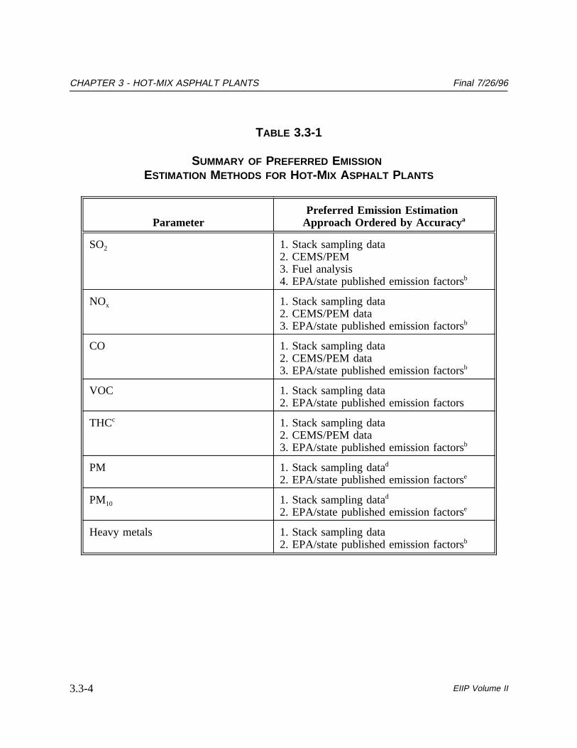
Table 3.3-1 identifies the preferred and alternative emission estimation approach(s) forselected pollutants. Table 3.3-1 is ordered according to the accuracy of the emissionestimation approach. The reader and the local air pollution agency must decide whichemission estimation approach is applicable based on costs and air pollution controlrequirements in their area. The preferred method chosen should also recognize the timespecificity of the emission estimate and the data quality. The quality of the data will dependon a variety of factors including the number of data points generated, the representativenessof those data points, and the proper operation and maintenance of the equipment being usedto record the measurements.
3.2.1 STACK SAMPLING
Without considering cost, stack sampling is the preferred emission estimation methodologyfor process NOx, CO, VOC, THC, PM, PM10, metals and speciated organics. EPA referencemethods and other methods of known quality can be used to obtain accurate estimates ofemissions at a given time for a particular facility.
3.2.2 EMISSION FACTORS
Due to their availability and acceptance in the industry, emission factors are commonly usedto prepare emission inventories. However, the emission estimate obtained from usingemission factors is based upon emissions testing performed at similar facilities and may notaccurately reflect emissions at a single source. Thus, the user should recognize that, in mostcases, emission factors are averages of available industry-wide data with varying degrees ofquality and may not be representative of averages for an individual facility within thatindustry. Emission factors are the preferred technique for estimating fugitive dust emissionsfor aggregate stockpiles and driving surfaces, as well as process fugitives.
3.2.3 FUEL ANALYSIS
Fuel analysis can be used as an approximation if no emission factors or site specific stacktest data are available. Once the concentration of sulfur in a fuel is known, SO2 emissionscan be calculated based on mass conservation laws, assuming negligible adsorption byalkaline aggregates.
EIIP Volume II 3.3-3
CHAPTER 3 - HOT-MIX ASPHALT PLANTS Final 7/26/96
TABLE 3.3-1
SUMMARY OF PREFERRED EMISSIONESTIMATION METHODS FOR HOT-MIX ASPHALT PLANTS
ParameterPreferred Emission Estimation
Approach Ordered by Accuracya
SO2 1. Stack sampling data2. CEMS/PEM3. Fuel analysis4. EPA/state published emission factorsb
NOx 1. Stack sampling data2. CEMS/PEM data3. EPA/state published emission factorsb
CO 1. Stack sampling data2. CEMS/PEM data3. EPA/state published emission factorsb
VOC 1. Stack sampling data2. EPA/state published emission factors
THCc 1. Stack sampling data2. CEMS/PEM data3. EPA/state published emission factorsb
PM 1. Stack sampling datad
2. EPA/state published emission factorse
PM10 1. Stack sampling datad
2. EPA/state published emission factorse
Heavy metals 1. Stack sampling data2. EPA/state published emission factorsb
EIIP Volume II3.3-4
Final 7/26/96 CHAPTER 3 - HOT-MIX ASPHALT PLANTS
TABLE 3.3-1
(CONTINUED)
ParameterPreferred Emission Estimation
Approach Ordered by Accuracya
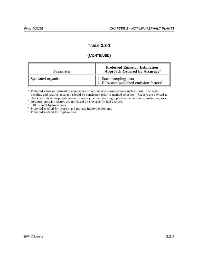
Speciated organics 1. Stack sampling data2. EPA/state published emission factorsb
a Preferred emission estimation approaches do not include considerations such as cost. The costs,benefits, and relative accuracy should be considered prior to method selection. Readers are advised tocheck with local air pollution control agency before choosing a preferred emission estimation approach.
b Assumes emission factors are not based on site-specific fuel analysis.c THC = total hydrocarbons.d Preferred method for process and process fugitive emissions.e Preferred method for fugitive dust.
EIIP Volume II 3.3-5

CHAPTER 3 - HOT-MIX ASPHALT PLANTS Final 7/26/96
3.2.4 CEMS AND PEM
HMA plants would not likely estimate emissions using CEMS and PEM. HMA plants haveconditions unfavorable to generating accurate CEM data including, high vibrations, highmoisture content of the stack gas, and dust. Nightly shutdown of CEMS would alsoadversely affect their performance. In some instances, however, CEMS may be used toestimate emissions of NOx, CO, and THC. This method may be used, for example, whendetailed records of emissions are needed over time. Similarly, stack gas flow rate may bemonitored using a continuous flow rate monitor, including pitot tubes, ultrasonic, and thermalmonitors (Patterson, 1995a).
PEM is a predictive emission estimation methodology whereby emissions are correlated toprocess parameters based on an initial series of stack tests at a facility. For example, VOCemissions may occur from asphalt mixtures produced at various temperatures with differentcombustion fuels and varying quantities of asphalt cement, aggregates, RAP, and crumbrubber. Similarly, sulfur dioxide emissions may be controlled by scrubbers that operate atvariable pressure drops, alkalinity, and recirculation rates. These parameters may bemonitored during the tests and correlated to the pollutant emission rates. Following thecorrelation development, parameters would be monitored to periodically predict emissionrates. Periodic stack sampling may be required to verify that the predictive emissioncorrelations are still accurate; if not, new correlations are developed.
EIIP Volume II3.3-6
4
PREFERRED METHODS FORESTIMATING EMISSIONSWithout consideration of cost, the preferred method for estimating emissions of mostpollutants emitted from HMA plants is the use of site-specific recent stack tests. Each statemay have a different preference or requirement and so it is suggested that the reader contactthe nearest state or local air pollution agency before deciding on which emission estimationmethodology to use. This section provides an outline for calculating emissions from HMAplants based on raw data collected by stack tests.
Table 3.4-1 lists the variables and symbols used in the following discussions.
4.1 EMISSION CALCULATIONS USING STACK SAMPLING DATA
Stack sampling test reports often provide emissions data in terms of lb/hr or grain/dscf.Annual emissions may be calculated from these data using Equations 3.4-1 or 3.4-2. Stacktests performed under a proposed permit condition or a maximum emissions rate are likely tobe higher than the emissions which would result under normal operating conditions. Theemission testing should only be completed after the purpose of the testing is known. Forexample, emission testing for particulate emissions may be different than emission testing forNew Source Performance Standards (NSPS) because the back-half catch portion is notconsidered.
This section shows how to calculate emissions in lb/hr based on stack sampling data.Calculations involved in determining particulate emissions from Method 5 data are used asan example. Because continuous PM monitors have not been demonstrated for this industry,the only available methods for measuring PM emissions are EPA Methods 5 or 17 and EPAMethod 201A for PM10. EPA Method 5 is used for NSPS testing. If condensible PM isneeded in the emissions estimate, the test method selected must be configured accordingly.
EIIP Volume II 3.4-1

CHAPTER 3 - HOT-MIX ASPHALT PLANTS Final 7/26/96
TABLE 3.4-1
LIST OF VARIABLES AND SYMBOLS
Variable Symbol Units
Concentration C parts per million volume dry (ppmvd)
Molecular weight MW lb/lb-mole
Molar volume V 385.5 ft3/lb-mole @ 68°F and 1 atmosphere
Flow rate Qa actual cubic feet per minute (acfm)
Flow rate Qd dry standard cubic feet per minute (dscfm)
Emissions Ex typically lb/hr of pollutant x
Annual emissions Etpy,x ton/year of pollutant x
Filter catch Cf grams (g)
Fuel use Qf typically, lb/hr
PM concentration CPM grain/dscf
Metered volume atstandard temperature andpressure
Vm,STP dscf
Moisture R percent
Temperature T degrees fahrenheit
Asphalt production A ton/hr
Annual operating hours OpHrs hr/yr
EIIP Volume II3.4-2

Final 7/26/96 CHAPTER 3 - HOT-MIX ASPHALT PLANTS
An example summary of a Method 5 test is shown in Table 3.4-2. The table shows theresults of three different sampling runs conducted during one test event. The sourceparameters measured as part of a Method 5 run include gas velocity and moisture content,which are used to determine exhaust gas flow rates in dscfm. The filter weight gain isdetermined gravimetrically and divided by the volume of gas sampled (as shown in Equation3.4-1) to determine the PM concentration in grains per dscf. Note that this example does notpresent the condensible PM emissions.
Pollutant concentration is then multiplied by the volumetric flow rate to determine theemission rate in pounds per hour, as shown in Equation 3.4-2 and Example 3.4-1.
where:
(3.4-1)CPM Cf/Vm,STP 15.43
CPM = concentration of PM or grain loading (grain/dscf)Cf = filter catch (g)Vm,STP = metered volume of sample at STP (dscf)15.43 = 15.43 grains per gram
where:
(3.4-2)EPM CPM Qd 60/7000
EPM = hourly emissions in lb/hr of PMQd = stack gas volumetric flow rate (dscfm)60 = 60 min/hr7000 = 7000 grains per pound
EIIP Volume II 3.4-3

CHAPTER 3 - HOT-MIX ASPHALT PLANTS Final 7/26/96
TABLE 3.4-2
TEST RESULTS - METHOD 5
Parameter Symbol Run 1 Run 2 Run 3
Total sampling time(minutes)
min 120 120 120
Moisture collected(grams)
g 395.6 372.6 341.4
Filter catch (grams) Cf 0.0851 0.0449 0.0625
Average samplingrate (dscfm)
dscfm 0.34 0.34 0.34
Standard meteredvolume, (dscf)
Vm,STP 41.83 40.68 40.78
Volumetric flow rate(acfm or dscfm)
Qa or Qd 17,972 17,867 17,914
Concentration ofparticulate(grains/dscf)
CPM 0.00204 0.00110 0.00153
Particulate emissionrate (lb/hr)
EPM 4.84 2.61 3.63
EIIP Volume II3.4-4

Final 7/26/96 CHAPTER 3 - HOT-MIX ASPHALT PLANTS
Example 3.4-1
PM emissions calculated using Equations 3.4-1 and 3.4-2 and the stack samplingdata for Run 1 (presented in Table 3.4-2 are shown below).
CPM = Cf/Vm,STP * 15.43= (0.085/41.83) * 15.43= 0.03 grain/dscf
EPM = CPM * Qd * 60/7000= 0.03 * 17,972 * (60 min/hr) * (1 lb/7000 grains)= 4.84 lb/hr
The information from some stack tests may be reported in pounds of particulate per poundsof exhaust gas (wet). Use Equation 3.4-3 to calculate the dry particulate emissions in lb/hr.
EPM = Qa/1000 * 60 * 0.075 (1 - R) * (528/460 + T) (3.4-3)
where:
EPM = hourly emissions in lb/hr PMQa = actual cubic feet of exhaust gas per minute (acfm)1000 = 1000 lb exhaust gas per lb of PM60 = 60 min/hr0.075 = 0.075 lb/ft3
R = moisture percent (%)528 = 528°F460 = 460°FT = stack gas temperature in °F
4.2 EMISSION FACTOR CALCULATIONS
Emission factors are commonly used to calculate emissions for fugitive dust sources andwhen site-specific monitoring data are unavailable. EPA maintains a compilation of emissionfactors inAP-42 for criteria pollutants and HAPs (EPA, 1995a). A supplementary source fortoxic air pollutant emission factors is the Factor Information and Retrieval (FIRE) datasystem (EPA, 1994). FIRE also contains emission factors for criteria pollutants.
EIIP Volume II 3.4-5

CHAPTER 3 - HOT-MIX ASPHALT PLANTS Final 7/26/96
Much work has been done recently on developing emission factors for HAPs and recentAP-42 revisions have included these factors (EPA, 1995a,b). In addition, many states havedeveloped their own HAP emission factors for certain source categories and require their usein any inventories including HAPs. Refer to Chapter 1 of Volume III for a completediscussion of available information sources for locating, developing, and using emissionfactors as an estimation technique.
Emission factors developed from measurements for a specific mixer or dryer may sometimesbe used to estimate emissions at other sites. For example, a company may have several unitsof similar model and size; if emissions were measured from one dryer or mixer, an emissionfactor could be developed and applied other similar units. It is advisable to have theemission factor reviewed and approved by state/local agencies or the EPA prior to its use.
The basic equation for using an emission factor to calculate emissions is the following:
where:
(3.4-4)Ex EFx Activity or Production Rate
Ex = emissions of pollutant xEFx = emission factor of pollutant x
Calculations using emission factors are presented in Examples 3.4-2 and 3.4-3.
4.3 EMISSION CALCULATIONS USING FUEL ANALYSIS DATA
Fuel analysis can be used to predict SO2 and other emissions based on application ofconservation laws, if fuel rate (Qf) is measured. The presence of certain elements in fuelsmay be used to predict their presence in emission streams. This includes elements such assulfur which may be converted to other compounds during the combustion process.
EIIP Volume II3.4-6

Final 7/26/96 CHAPTER 3 - HOT-MIX ASPHALT PLANTS
Example 3.4-2
Example 3.4-2 shows how potential hourly VOC combustion emissions may becalculated for a parallel flow drum mixer using a total organic compound (TOC)emission factor fromAP-42, Table 11.1-8, for an oil-fired dryer. The asphalt plantis assumed to operate 1,200 hours per year.
EFTOC = 0.069 lb/ton asphalt produced
Maximum asphalt production rate = 350 ton/hr
TOC emissions = EFTOC * asphalt production rate= 0.069* 350= 24.15 lb/hr * 1 ton/2000 lb * 1200 hr/yr= 14.5 ton/yr
Example 3.4-3
Example 3.4-3 shows how potential hourly xylene emissions may be calculated fora batch mix HMA plant with a natural gas-fired dryer based on a xylene emissionfactor fromAP-42, Table 11.1-9. The HMA plant is assumed to operate 1,200hours per year.
EFxylene = 0.0043 lb/ton asphalt produced
Xylene emissions = EFxylene * maximum asphalt production rate= (0.0043 lb/ton)* 350 ton/hr= 1.5 lb/hr * 1 ton/2000 lb * 1200 hr/yr= 0.9 ton/yr
The basic equation used in fuel analysis emission calculations is the following:
(3.4-4)Ex = Qf Pollutant concentration in fuel
MWp
MWf
EIIP Volume II 3.4-7
CHAPTER 3 - HOT-MIX ASPHALT PLANTS Final 7/26/96
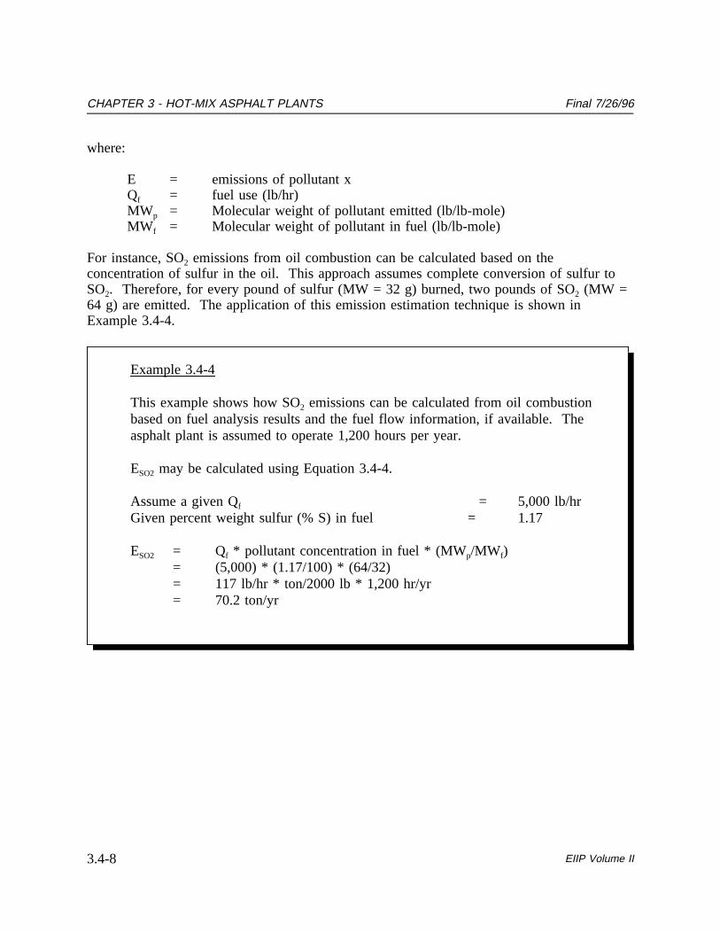
where:
E = emissions of pollutant xQf = fuel use (lb/hr)MWp = Molecular weight of pollutant emitted (lb/lb-mole)MWf = Molecular weight of pollutant in fuel (lb/lb-mole)
For instance, SO2 emissions from oil combustion can be calculated based on theconcentration of sulfur in the oil. This approach assumes complete conversion of sulfur toSO2. Therefore, for every pound of sulfur (MW = 32 g) burned, two pounds of SO2 (MW =64 g) are emitted. The application of this emission estimation technique is shown inExample 3.4-4.
Example 3.4-4
This example shows how SO2 emissions can be calculated from oil combustionbased on fuel analysis results and the fuel flow information, if available. Theasphalt plant is assumed to operate 1,200 hours per year.
ESO2 may be calculated using Equation 3.4-4.
Assume a given Qf = 5,000 lb/hrGiven percent weight sulfur (% S) in fuel = 1.17
ESO2 = Qf * pollutant concentration in fuel * (MWp/MWf)= (5,000) * (1.17/100) * (64/32)= 117 lb/hr * ton/2000 lb * 1,200 hr/yr= 70.2 ton/yr
EIIP Volume II3.4-8

5
ALTERNATIVE METHODS FORESTIMATING EMISSIONS
5.1 EMISSION CALCULATIONS USING CEMS DATA
To monitor SO2, NOx, THC, and CO emissions using a CEMS, a facility uses a pollutantconcentration monitor, which measures concentration in parts per million by volume dry air(ppmvd). Note that a CEMS would not likely be used to monitor emissions for an extendedperiod due to the unfavorable conditions at an HMA plant. Flow rates should be measuredusing a volumetric flow rate monitor. Flow rates estimated based on heat input using fuelfactors may be inaccurate because these systems typically run with high excess air to removethe moisture out of the drum (Patterson, 1995). Emission rates (lb/hr) are then calculated bymultiplying the stack gas concentrations by the stack gas flow rates.
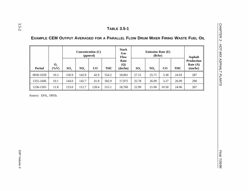
Table 3.5-1 presents example CEMS data output averaged for three periods for a parallelflow drum mixer. The output includes pollutant concentrations in parts per million dry basis(ppmvd), diluent (O2 or CO2) concentrations in percent by volume dry basis (%v,d), andemission rates in pounds per hour (lb/hr). These data represent a "snapshot" of a drum mixeroperation. While it is possible to determine total emissions of an individual pollutant over agiven time period from these data assuming the CEM operates properly all year long, anaccurate emission estimate can be made by summing the hourly emission estimates if theCEMS data are representative of typical operating conditions.
Although CEMS can report real-time hourly emissions automatically, it may be necessary tomanually estimate annual emissions from hourly concentration data. This section describeshow to calculate emissions from CEMS concentration data. The selected CEMS data shouldbe representative of operating conditions. When possible, data collected over longer periodsshould be used. It is important to note that prior to using CEMS to estimate emissions, aprotocol should be developed for collecting and averaging the data.
EIIP Volume II 3.5-1
CH
AP
TE
R3
-H
OT
-MIX
AS
PH
ALT
PLA
NT
SF
inal7/26/96TABLE 3.5-1
EXAMPLE CEM OUTPUT AVERAGED FOR A PARALLEL FLOW DRUM MIXER FIRING WASTE FUEL OIL
PeriodO2
(%V)
Concentration (C)(ppmvd)
StackGasFlowRate(Q)
(dscfm)
Emission Rate (E)(lb/hr) Asphalt
ProductionRate (A)(ton/hr)SO2 NOx CO THC SO2 NOx CO THC
0830-1039 10.3 150.9 142.9 42.9 554.2 18,061 27.15 25.71 3.38 24.93 287
1355-1606 10.1 144.0 145.7 41.8 582.9 17,975 25.78 26.09 3.27 26.09 290
1236-1503 11.8 123.0 112.7 128.4 515.1 18,760 22.99 21.06 10.50 24.06 267
Source: EPA, 1991b.
EIIP
Volum
eII
3.5-2

Final 7/26/96 CHAPTER 3 - HOT-MIX ASPHALT PLANTS
Hourly emissions can be based on concentration measurements as shown in Equation 3.5-1and Example 3.5-1.
where:
(3.5-1)Ex = (C MW Q 60)
(V 106)
Ex = hourly emissions in lb/hr of pollutant xC = pollutant concentration in ppmvdMW = molecular weight of the pollutant (lb/lb-mole)Q = stack gas volumetric flow rate in dscfm60 = 60 min/hrV = volume occupied by one mole of ideal gas at standard
temperature and pressure (385.5 ft3/lb-mole @ 68°F and 1 atm)
Actual emissions in tons per year can be calculated by multiplying the emission rate in lb/hrby the number of actual annual operating hours (OpHrs) as shown in Equation 3.5-2 andExample 3.5-1.
where:
(3.5-2)Etpy,x = Ex OpHrs/2000
Etpy,x = annual emissions in ton/yr of pollutant xEx = hourly emissions in lb/hr of pollutant xOpHrs = annual operating hours in hr/yr
Emissions in pounds of pollutant per ton of asphalt produced can be calculated by dividingthe emission rate in lb/hr by the asphalt production in rate (ton/hr) during the same period(Equation 3.5-3) as shown below. It should be noted that the emission factor calculatedbelow assumes that the selected period (i.e., hour) is representative of annual operatingconditions and longer time periods should be used when available. Use of the calculation isshown in Example 3.5-1.
(3.5-3)Etpy,x Ex/A
EIIP Volume II 3.5-3

CHAPTER 3 - HOT-MIX ASPHALT PLANTS Final 7/26/96
where:
Etpy,x = emissions of pollutant x (lb/ton) per ton of asphalt producedEx = hourly emissions in lb/hr of pollutant xA = asphalt production (ton/hr)
5.2 PREDICTIVE EMISSION MONITORING
Example 3.5-1
This example shows how SO2 emissions can be calculated using Equation 3.5-1based on the average CEMS data for 8:30-10:39 shown in Table 3.5-1.
ESO2 ===
(C * MW * Q * 60)/(V * 106)150.9 * 64 * 18,061 * 60/(385.5 * 106)27.15 lb/hr
Emissions in ton/yr (based on a 1,200 hr/yr operating schedule) can then becalculated using Equation 3.5-2; however, based on the above period this estimateshould be calculated from the average CEMS data for year using Equation 3.5-1:
Etpy,SO2 = ESO2 * OpHrs/2,000= 27.15 * (1,200/2,000)= 16.29 ton/yr
Emissions, in terms of lb/ton asphalt produced, are calculated using Equation 3.5-3:
Etpy,SO2 = ESO2/A= 9.46 * 10-2 lb SO2/ton asphalt produced
Emissions from the HMA process depend upon several variables, which are discussed inSection 3 of this chapter. For example, VOC process emissions for a given plant may varywith several parameters, including: the type of fuel burned; the relative quantities of asphaltconstituents (e.g., RAP, crumb rubber, and emulsifiers); aggregate type and moisture content;the temperature of the asphalt constituents; the mixing zone temperature; and, fuelcombustion rate. An example emissions monitoring that could be used to develop a PEM
EIIP Volume II3.5-4
Final 7/26/96 CHAPTER 3 - HOT-MIX ASPHALT PLANTS
protocol would need to account for the variability in these parameters and, consequently, mayrequire a complex testing algorithm.
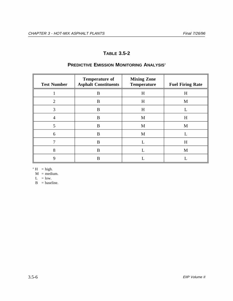
To develop this algorithm, correlation testing of the process variables could be conductedover a range of potential operating conditions using EPA Method 25 or Method 25A tomeasure THC emissions and EPA Method 6A or Method 6C to measure SO2 emissions.Potential testing conditions covering several parameters are shown in Table 3.5-2. Based onthe test data, a mathematical correlation can be developed which predicts emissions usingthese parameters. This method may be cost prohibitive for a single source.
EIIP Volume II 3.5-5
CHAPTER 3 - HOT-MIX ASPHALT PLANTS Final 7/26/96
TABLE 3.5-2
PREDICTIVE EMISSION MONITORING ANALYSISa
Test NumberTemperature of
Asphalt ConstituentsMixing ZoneTemperature Fuel Firing Rate
1 B H H
2 B H M
3 B H L
4 B M H
5 B M M
6 B M L
7 B L H
8 B L M
9 B L L
a H = high.M = medium.L = low.B = baseline.
EIIP Volume II3.5-6
6
QUALITY ASSURANCE/QUALITYCONTROLThe consistent use of standardized methods and procedures is essential in the compilation ofreliable emission inventories. QA and QC of an inventory is accomplished through a set ofprocedures that ensure the quality and reliability of data collection and analysis. Theseprocedures include the use of appropriate emission estimation techniques, applicable andreasonable assumptions, accuracy/logic checks of computer models, checks of calculations,and data reliability checks. Figure 3.6-1 provides an example checklist that could aid theinventory preparer at a HMA plant. Volume VI,QA Proceduresof this series describesadditional QA/QC methods and tools for performing these procedures.
Volume II, Chapter 1,Introduction to Stationary Point Source Emission InventoryDevelopment, presents recommended standard procedures to follow that ensure the reportedinventory data are complete and accurate. The QA/QC section of Chapter 1 should beconsulted for current EIIP guidance for QA/QC checks for general procedures, recommendedcomponents of a QA plan, and recommended components for point source inventories. TheQA plan discussion includes recommendations for data collection, analysis, handling, andreporting. The recommended QC procedures include checks for completeness, consistency,accuracy, and the use of approved standardized methods for emission calculations, whereapplicable. Chapter 1 also describes guidelines to follow in order to ensure the quality andvalidity of the data from manual and continuous emission monitoring methodologies used toestimate emissions.
6.1 CONSIDERATIONS FOR USING STACK TEST AND CEMS DATA
Data collected via CEMS, PEM, or stack tests must meet quality objectives. Stack test datamust be reviewed to ensure that the test was conducted under normal operating conditions, orunder maximum operating conditions in some states, and that it was generated according toan acceptable method for each pollutant of interest. Calculation and interpretation ofaccuracy for stack testing methods and CEMS are described in detail inQuality AssuranceHandbook for Air Pollution Measurements Systems: Volume III. Stationary Source SpecificMethods (Interim Edition).
The acceptance criteria, limits, and values for each control parameter associated with manualsampling methods, such as dry gas meter calibration and leak rates, are summarized withinthe tabular format of the QA/QC section of Chapter 1. QC procedures for all instruments
EIIP Volume II 3.6-1

CHAPTER 3 - HOT-MIX ASPHALT PLANTS Final 7/26/96
Item Y/N
Corrective Action(complete if "N";
describe, sign, and date)
1. Have the toxic emissions been calculated andreported using approved stack test methods or usingthe emission factors provided fromAP-42, FIRE,and/or NAPA (National Asphalt PavementAssociation)? Have asphalt production rates beenincluded? Each facility should request from theirstate agency guidance on which test methods oremission factors should be used.
2. Fugitive emissions are required for the inventory,but will not count towards a Title V determinationunless the facility is NSPS affected. Presently, inthe case of the asphalt plants, only particulateemissions for the process as defined in 40 CFR60.90 are NSPS affected. Have fugitive emissionsbeen calculated?
3. If emission factors are used to calculate fuel usageemissions, have fuel usage rates been determined forthe dryer and for the asphalt heater separately? Ifthe AP-42dryer emission factors are used, theyalready contain emissions from fuel combustion inthe dryer.
4. Again, request guidance from the state regulatoryagency on whether or not to calculate toxicemissions from fuel usage. Most toxic emissionfactors usually are inclusive of the asphalt and thefuel. Has the state agency been contacted forguidance?
5. Have stack parameters been provided for each stackor vent which emits criteria or toxic pollutants?This includes the fabric filter or scrubber installedon the asphalt dryer/mixer, the asphalt cementheaters, and any storage silos other than asphaltconcrete storage.
FIGURE 3.6-1. EXAMPLE EMISSION INVENTORY DEVELOPMENTCHECKLIST FOR ASPHALT PLANTS
EIIP Volume II3.6-2

Final 7/26/96 CHAPTER 3 - HOT-MIX ASPHALT PLANTS
Item Y/N
Corrective Action(complete if "N";
describe, sign,and date)
6. Check with the state regulatory agency to determinewhether emissions should be calculated usingAP-42emission factors:
Dryer/Mix Type:
Rotary Dryer (Batch Mix): Conventional Plant(3-05-002-01)Drum (Mix) Dryer: Hot Asphalt Plant (3-05-002-05)
Diesel Generators: Industrial diesel reciprocating(2-02-001-02)
Asphalt Heaters:
"In Process Fuel Use Factors" (Residual, 3-05-002-07;Distillate, 3-05-002-08; Natural Gas, 3-05-002-06; LPG,3-05-002-09).
7. Have you considered storage piles (3-05-002-03)(includeshandling of piles) from both Batch and Drum Plants?
8. If required by the state, has a site diagram been includedwith the emission inventory? This should be a detailedplant drawing showing the location of sources/stacks withID numbers for all processes, control equipment, andexhaust points.
9. Have examples of all calculations been included?
10. Have all conversions and units been reviewed and checkedfor accuracy?
FIGURE 3.6-1. (CONTINUED)
EIIP Volume II 3.6-3

CHAPTER 3 - HOT-MIX ASPHALT PLANTS Final 7/26/96
used to continuously collect emissions data are similar. The primary control check forprecision of the continuous monitors is daily analysis of control standards. The CEMSacceptance criteria and control limits are listed within the tabular format of the QA/QCsection of Chapter 1.
Quality assurance should be delineated in a Quality Assurance Plan (QAP) by the teamconducting the test prior to each specific test. The main objective of any QA/QC effort forany program is to independently assess and document the precision, accuracy, and adequacyof emission data generated during sampling and analysis. It is essential that the emissionsmeasurement program be performed by qualified personnel using proper test equipment.Also, valid test results require the use of appropriate and properly functioning test equipmentand use of appropriate reference methods.
The QAP should be developed to assure that all testing and analytical data generated arescientifically valid, defensible, comparable, and of known and acceptable precision andaccuracy. EPA guidance, is available for assistance in preparing any QAP (EPA, October,1989).
6.2 CONSIDERATIONS FOR USING EMISSION FACTORS
The use of emission factors is straightforward when the relationship between process dataand emissions is direct and relatively uncomplicated. When using emission factors, the usershould be aware of the quality indicator associated with the value. Emission factorspublished within EPA documents and electronic tools have a quality rating applied to them.The lower the quality indicator, the more likely that a given emission factor may not berepresentative of the source type. When an emission factor for a specific source or categorymay not provide a reasonably adequate emission estimate, it is always better to rely on actualstack test or CEMS data, where available. The reliability and uncertainty of using emissionfactors as an emission estimation technique are discussed in detail in the QA/QC Section ofChapter 1.
6.3 DATA ATTRIBUTE RATING SYSTEM (DARS) SCORES
One measure of emission inventory data quality is the DARS score. Four examples aregiven here to illustrate DARS scoring using the preferred and alternative methods. TheDARS provides a numerical ranking on a scale of 1 to 10 for individual attributes of theemission factor and the activity data. Each score is based on what is known about the factorand the activity data, such as the specificity to the source category and the measurementtechnique employed. The composite attribute score for the emissions estimate can be viewedas a statement of the confidence that can be placed in the data. For a complete discussion ofDARS and other rating systems, see theQA Source Document(Volume VI, Chapter 4) and
EIIP Volume II3.6-4

Final 7/26/96 CHAPTER 3 - HOT-MIX ASPHALT PLANTS
the QA/QC Section within Volume II Chapter 1,Introduction to Stationary Point SourcesEmission Inventory Development.
Each of the examples below is hypothetical. A range is given where appropriate to coverdifferent situations. The scores are assumed to apply to annual emissions from an HMAplant. Table 3.6-1 gives a set of scores for an estimate based on CEMS/PEM data. Aperfect score of 1.0 is achievable using this method if data quality is very good. Note thatmaximum scores of 1.0 are automatic for the source definition and spatial congruityattributes. Likewise, the temporal congruity attribute receives a 1.0 if data capture is greaterthan 90 percent; this assumes that data are sampled adequately throughout the year. Themeasurement attribute score of 1.0 assumes that the pollutants of interest were measureddirectly. A lower score is given if the emissions are speciated using a profile, or if theemissions are used as a surrogate for another pollutant. Also, the measurement/method scorecan be less than 1.0 if the relative accuracy is poor (e.g., >10 percent), if the data are biased,or if data capture is closer to 90 percent than to 100 percent.
The use of stack sample data can give DARS scores as high as those for CEMS/PEM data.However, the sample size is usually too low to be considered completely representative ofthe range of possible emissions making a score of 1.0 for measurement/method unlikely. Atypical DARS score for stack sample data is generally closer to the low end of the rangeshown in Table 3.6-2.
Two examples are given for emissions calculated using emission factors. For both of theseexamples, the activity data is assumed to be measured directly or indirectly. Table 3.6-3applies to an emission factor developed from CEMS/PEM data from one dryer or mixer andthen applied to a different dryer or mixer of similar design and age. Table 3.6-4 gives anexample for an estimate made with anAP-42emission factor. TheAP-42 factor is a meanand could overestimate or underestimate emissions for anysingle unit in the population. Thus, the confidence that can be placed in emissions estimatedfor a specific unit with a generalAP-42 factor is lower than emissions based on source-specific data. This assumes that the source-specific data were developed while the HMAplant was operating under normal conditions. If it was not operated under normal conditionsthen theAP-42emission factor may be a better characterization of the emissions from theHMA plant.
The example in Table 3.6-3 shows that emission factors based on high-quality data from asimilar unit will typically give better results than a general factor. The main criterionaffecting the score is how similar the unit used to generate the factor is to the target dryer ormixer.If sufficient data are available, the uncertainty in the estimate should be quantified. Ifsufficient data are not available, a qualitative analysis of uncertainty is still recommended.Some methods and examples are described inQA Procedures(Volume VI, Chapter 3).
EIIP Volume II 3.6-5

CHAPTER 3 - HOT-MIX ASPHALT PLANTS Final 7/26/96
TABLE 3.6-1
DARS SCORES: CEMS/PEM DATAa
Attribute
EmissionFactorScore
ActivityData Score
Composite Scores
CommentRange Midpoint
Measurement/method
0.9 - 1.0 0.9 - 1.0 0.81 - 1.0 0.91 Lower scores given ifrelative accuracy poor(e.g.,>10 percent) or datacapture closer to90 percent.
Source definition 1.0 1.0 1.0 - 1.0 1.0
Spatial congruity 1.0 1.0 1.0 - 1.0 1.0
Temporalcongruity
1.0 1.0 1.0 - 1.0 1.0
Weighted Score 0.98 - 1.0 0.98 - 1.0 0.95 - 1.0 0.98
a Assumes data capture is 90 percent or better, representative of entire year, monitors sensors, andother equipment is properly maintained.
EIIP Volume II3.6-6

Final 7/26/96 CHAPTER 3 - HOT-MIX ASPHALT PLANTS
TABLE 3.6-2
DARS SCORES: STACK SAMPLE DATAa
Attribute
EmissionFactorScore
ActivityData Score
Composite Scores
CommentRange Midpoint
Measurement/method
0.7 - 1.0 0.7 - 1.0 0.49 - 1.0 0.745
Source definition 1.0 - 1.0 1.0 - 1.0 1.0 - 1.0 1.0
Spatial congruity 1.0 - 1.0 1.0 - 1.0 1.0 - 1.0 1.0
Temporalcongruity
0.7 - 1.0 0.7 - 1.0 0.49 - 1.0 0.745 Lower scores givenif emissions varytemporally andsample does notcover range.
Weighted Score 0.85 - 1.0 0.85 - 1.0 0.75 - 1.0 0.878
a Assumes use of EPA Reference Method, high quality data.
EIIP Volume II 3.6-7
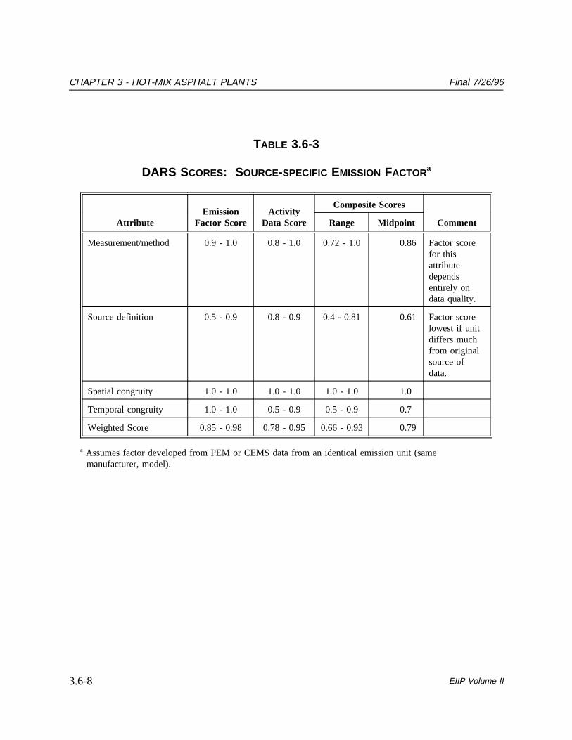
CHAPTER 3 - HOT-MIX ASPHALT PLANTS Final 7/26/96
TABLE 3.6-3
DARS SCORES: SOURCE-SPECIFIC EMISSION FACTORa
AttributeEmission
Factor ScoreActivity
Data Score
Composite Scores
CommentRange Midpoint
Measurement/method 0.9 - 1.0 0.8 - 1.0 0.72 - 1.0 0.86 Factor scorefor thisattributedependsentirely ondata quality.
Source definition 0.5 - 0.9 0.8 - 0.9 0.4 - 0.81 0.61 Factor scorelowest if unitdiffers muchfrom originalsource ofdata.
Spatial congruity 1.0 - 1.0 1.0 - 1.0 1.0 - 1.0 1.0
Temporal congruity 1.0 - 1.0 0.5 - 0.9 0.5 - 0.9 0.7
Weighted Score 0.85 - 0.98 0.78 - 0.95 0.66 - 0.93 0.79
a Assumes factor developed from PEM or CEMS data from an identical emission unit (samemanufacturer, model).
EIIP Volume II3.6-8

Final 7/26/96 CHAPTER 3 - HOT-MIX ASPHALT PLANTS
TABLE 3.6-4
DARS SCORES: AP-42 EMISSION FACTORa
AttributeEmission
Factor ScoreActivity
Data Score
Composite Scores
CommentRange Midpoint
Measurement/method 0.6 - 0.8 0.8 - 1.0 0.48 - 0.7 0.59 Score dependson quality andquantity ofdata pointsused todevelopfactor.
Source definition 0.5 - 0.9 0.8 - 0.9 0.4 - 0.81 0.605 Emissionfactor scorewill be low ifvariability insourcepopulation ishigh.
Spatial congruity 0.6 - 0.8 1.0 - 1.0 0.6 - 0.8 0.7 Factor scorelower ifgeographiclocation hassignificanteffect onemissions.
Temporal congruity 0.5 - 0.9 0.5 - 0.9 0.25 - 0.81 0.53 Lower scoresgiven ifemissionsvarytemporallyand sampledoes not coverrange.
Weighted Score 0.55 - 0.85 0.78 - 0.95 0.43 - 0.78 0.61
a Assumes activity data (e.g., fuel use) or surrogate is measured directly in some manner.
EIIP Volume II 3.6-9
CHAPTER 3 - HOT-MIX ASPHALT PLANTS Final 7/26/96
The reader should note that the presentation of the DARS scores here is shown as ahypothetical example, only. Although the highest DARS score results from the use ofCEMS, this estimation technique will not practically be applied or used by the majority offacilities operating. Due to technical feasibility issues and costs incurred by applying CEMSto a HMA plant, stack testing or emission factors may provide the best choice when selectingan appropriate method for estimating emissions (even though stack testing or emissionfactors did not receive the highest DARS score). The reader should always contact theirstate regulatory agency for approval of selected methodologies or techniques. Also, it shouldbe noted that this hypothetical application of DARS does not mandate any emissionestimation method, but only offers the reader a means for selecting any one method overanother.
EIIP Volume II3.6-10

7
DATA CODING PROCEDURESThis section describes the methods and codes available for characterizing emission sources atHMA facilities. Consistent categorization and coding will result in greater uniformity amonginventories. The SCCs are the building blocks on which point source emissions data arestructured. Each SCC represents a unique process or function within a source category thatis logically associated with an emission point. Without an appropriate SCC, a process cannotbe accurately identified for retrieval purposes. In addition, the procedures described herewill assist the reader preparing data for input to the Aerometric Information Retrieval System(AIRS) or a similar database management system. For example, the use of the SCCsprovided in Table 3.7-1 are recommended for describing HMA operations. Refer toCHIEF for a complete listing of SCCs for HMA plants. While the codespresented here are currently in use, they may change based on further refinement by theemission inventory user community. As part of the EIIP, a common emissions dataexchange format is being developed to facilitate data transfer between industry, states, andEPA. Details on SCCs for specific emission sources are as follows:
Process Emissions: For asphaltic concrete production processes, be careful to useonly one SCC for each process. Use the codes for either the batch or continuousprocess or for the drum mix process, depending on which process is used. Theprocess-specific codes should be used as often as possible; however, "Entire Unit" and"General" codes are available. If the "Entire Unit" code is used, do not use thechemical-specific or process-specific codes as this would double-count emissions.AP-42 emission factors for dryer emissions include all stack emissions (including productsof combustion from the dryer burner).
In-Process Fuel: In-process fuel includes SCCs for asphalt cement heaters. Theseemissions are separate and apart from dryer emissions.
Generators: Diesel generators may be used at portable HMA plants to generateelectricity. These emissions are not included in emission factors for processemissions.
EIIP Volume II 3.7-1

CHAPTER 3 - HOT-MIX ASPHALT PLANTS Final 7/26/96
Storage Tanks: Storage tanks may be used in the asphaltic concrete productionprocess to store fuel such as oil. Potential emissions from storage tanks will likely beinsignificant. The codes in Table 3.7-1 are recommended to describe fuel storageemissions.
Fugitive Emissions: Fugitive emissions from asphaltic concrete production resultprimarily from the storage and handling of raw materials and finished product. Themiscellaneous codes may be used for fugitive emission sources without a uniquecode. Remember to use the comment section to describe the emissions.
Control device codes applicable to asphaltic concrete production are presented in Table 3.7-2.These should be used to enter the type of applicable emissions control device into the AIRSFacility Subsystem (AFS). The "099" control code may be used for miscellaneous controldevices that do not have a unique identification code.
If there are significant sources of fugitive emissions within the facility, or sources that havenot been specifically discussed thus far, they should be included in the emissions estimates ifrequired by the state. Conditions vary from plant to plant, thus, each specific case cannot bediscussed within the context of this document.
EIIP Volume II3.7-2

Final 7/26/96 CHAPTER 3 - HOT-MIX ASPHALT PLANTS
TABLE 3.7-1
SOURCE CLASSIFICATION CODES FOR ASPHALTIC CONCRETEPRODUCTION (SIC CODE 2951)
Source Description Process Description SCC Units
Process Emissions
Batch or continuousmix process
Rotary dryer 3-05-002-01 Tons HMA produced
Hot elevators, screens, bins, andmixer
3-05-002-02 Tons aggregateprocessed
Drum mix process Drum mixer: hot asphalt plants 3-05-002-05 Tons HMA produced
General process General process/specify incomments
3-05-002-99 Tons produced
In-place recycling - propane 3-05-002-15 Tons produced
In-Process Fuel
Asphalt heater fueluse
Residual oil 3-05-002-07 1000 gallons burned
Distillate oil 3-05-002-08 1000 gallons burned
Natural gas 3-05-002-06 Million ft 3 burned
Waste oil 3-05-002-10 1000 gallons burned
Liquid petroleum gas 3-05-002-09 1000 gallons burned
Generators
Diesel Reciprocating 2-02-001-02 Horsepower hours
Fugitive Emissions
Fugitive emissions Raw material storage piles 3-05-002-03 Tons aggregateprocessed
Cold aggregate handling 3-05-002-04 Tons aggregateprocessed
Storage silo 3-05-002-13 Tons HMA produced
Truck load-out 3-05-002-14 Tons HMA loaded
Miscellaneous fugitive emissions 3-05-888-01 to 05 Vehicle milestravelled
Haul roads - general 3-05-002-90 Tons product
EIIP Volume II 3.7-3
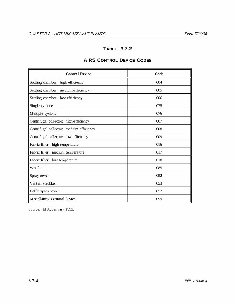
CHAPTER 3 - HOT-MIX ASPHALT PLANTS Final 7/26/96
TABLE 3.7-2
AIRS CONTROL DEVICE CODES
Control Device Code
Settling chamber: high-efficiency 004
Settling chamber: medium-efficiency 005
Settling chamber: low-efficiency 006
Single cyclone 075
Multiple cyclone 076
Centrifugal collector: high-efficiency 007
Centrifugal collector: medium-efficiency 008
Centrifugal collector: low-efficiency 009
Fabric filter: high temperature 016
Fabric filter: medium temperature 017
Fabric filter: low temperature 018
Wet fan 085
Spray tower 052
Venturi scrubber 053
Baffle spray tower 052
Miscellaneous control device 099
Source: EPA, January 1992.
EIIP Volume II3.7-4

8
REFERENCESCode of Federal Regulations. July 1, 1987. Title 40, Part 60, Appendix A. Office of theFederal Register, Washington, DC.
EIIP. March 1995. Preferred and Alternative Methods for Estimating Air Emissions fromBoilers, Review Draft. Emission Inventory Improvement Program, Point Sources Committee.Prepared under EPA Contract No. 68-D2-0160, Work Assignment No. 41.U.S. Environmental Protection Agency, Office of Air Quality Planning and Standards,Research Triangle Park, North Carolina.
EPA. 1986. Test Methods for Evaluating Solid Waste, Report No. SW-846, Third Edition.U.S. Environmental Protection Agency, Office of Solid Waste and Emergency Response,Washington, DC.
EPA. April 1989. Estimating Air Toxic Emissions from Coal and Oil Combustion Sources.EPA-450/2-89-001. U.S. Environmental Protection Agency, Office of Air Quality Planningand Standards, Research Triangle Park, North Carolina.
EPA. October 1989.Preparing Perfect Project Plans.EPA-600/9-89/087.U.S. Environmental Protection Agency, Risk Reduction Laboratory, Cincinnati, Ohio.
EPA. September 1991a.Emission Testing for Asphalt Concrete Industry. Site Specific TestPlan and Quality Assurance Project Plan. Mathy Construction Company Plant 6.U.S. Environmental Protection Agency, Office of Air Quality Planning and Standards,Research Triangle Park, North Carolina.
EPA. September 1991b.Asphalt Emission Test Report. Mathy Construction Company,LaCrosse, Wisconsin.U.S. Environmental Protection Agency, Office of Air Quality Planningand Standards, Research Triangle Park, North Carolina.
EPA. May 1991. Procedures for the Preparation of Emission Inventories for CarbonMonoxide and Precursors of Ozone.Volume I: General Guidance for Stationary Sources.U.S. Environmental Protection Agency, Office of Air Quality Planning and Standards,Research Triangle Park, North Carolina.
EIIP Volume II 3.8-1
CHAPTER 3 - HOT-MIX ASPHALT PLANTS Final 7/26/96
EPA. January 1992.AIRS User’s Guide, Volume XI: AFS Data Dictionary.U.S.Environmental Protection Agency, Office of Air Quality Planning and Standards, ResearchTriangle Park, North Carolina.
EPA. 1994. Factor Information and Retrieval (FIRE) Data System, Version 4.0.UpdatedAnnually. U.S. Environmental Protection Agency, Office of Air Quality Planning andStandards, Research Triangle Park, North Carolina.
EPA. January 1995a.Compilation of Air Pollutant Emission Factors. Volume I: StationaryPoint and Area Sources, Fifth Edition, AP-42. Section 11.1, Hot-Mix Asphalt Plants.U.S. Environmental Protection Agency, Office of Air Quality Planning and Standards,Research Triangle Park, North Carolina.
EPA. January 1995b.Compilation of Air Pollutant Emission Factors. Volume I. StationaryPoint and Area Sources, Fifth Edition, AP-42. Section 3.3-1, Stationary Internal CombustionSources. U.S. Environmental Protection Agency, Office of Air Quality Planning andStandards, Research Triangle Park, North Carolina.
EPA. January 1995c.Compilation of Air Pollutant Emission Factors. Volume I. StationaryPoint and Area Sources, Fifth Edition, AP-42. Section 1.11, Waste Oil Combustion.U.S.Environmental Protection Agency, Office of Air Quality Planning and Standards, ResearchTriangle Park, North Carolina.
Fore, Gary, of National Asphalt Pavement Association, Lanham, Maryland.Telecommunication with Robert Harrison, Radian Corporation. August 18, 1995.
Gunkel, Kathryn O’C. 1992.Hot-Mix Asphalt Mixing Facilities. Buonicore, Anthony J.,and Wayne T. Davis, Editors.Air Pollution Engineering Manual. Van Nostrand Reinhold,New York, New York.
Khan, Z.S., and T.W. Hughes. November 1977.Source Assessment: Asphalt Hot-Mix.EPA-600/2-77-107n. U.S. Environmental Protection Agency, Industrial EnvironmentalResearch Laboratory, Cincinnati, Ohio.
National Asphalt Pavement Association (NAPA). February 1995.Dealing with Title VOperating Permits: the Synthetic Minor Alternative.Special Report 175. Lanham,Maryland.
Nevers, Noel. 1995.Air Pollution Control Engineering. McGraw-Hill, Incorporated.
EIIP Volume II3.8-2
Final 7/26/96 CHAPTER 3 - HOT-MIX ASPHALT PLANTS
Patterson, Ralph, of Wisconsin Department of Natural Resources. May 2, 1995a.Memorandum to Theresa Kemmer Moody, Radian Corporation,Comments on Preferred andAlternative Methods for Estimating Air Emissions from Hot-Mix Asphalt Plants.
Patterson, Ralph, of Wisconsin Department of Natural Resources. June 16, 1995b.Telecommunication with Robert Harrison, Radian Corporation.
Patterson, Ralph, of Wisconsin Department of Natural Resources. October 26, 1995c.Memorandum to Theresa Kemmer Moody, Radian Corporation,Comments on Preferred andAlternative Methods for Estimating Air Emissions from Hot-Mix Asphalt Plants.
Stultz, Steven C., and John B. Kitto, Editors. 1992.Steam, Its Generation and Use. TheBabcock and Wilcox Company.
Texas Natural Resource Conservation Commission, Office of Air Quality. January 1994.Asphalt Concrete Plants: Emissions Calculations Instructions. Compiled by TNRCCMechanical Section Engineers, Austin, Texas.
Wiese, Lynda, of Wisconsin Department of Natural Resources. June 15, 1995.Memorandum to Theresa Kemmer Moody, Radian Corporation.Comments on Preferred andAlternative Methods for Estimating Air Emissions from Hot-Mix Asphalt Plants.
EIIP Volume II 3.8-3

CHAPTER 3 - HOT-MIX ASPHALT PLANTS Final 7/26/96
This page is intentionally left blank.
EIIP Volume II3.8-4

Final 7/26/96 CHAPTER 3 - HOT-MIX ASPHALT PLANTS
APPENDIX A
EXAMPLE DATA COLLECTION FORMAND INSTRUCTIONS FOR HOT-MIX
ASPHALT PLANTS
EIIP Volume II

CHAPTER 3 - HOT-MIX ASPHALT PLANTS Final 7/26/96
This page is intentionally left blank.
EIIP Volume II

Final 7/26/96 CHAPTER 3 - HOT-MIX ASPHALT PLANTS
EXAMPLE DATA COLLECTION FORMINSTRUCTIONS
1. This form may be used as a work sheet to aid the plant engineer in collecting theinformation necessary to calculate emissions from HMA plants. The informationrequested on the form relates to the methods (described in Sections 3 through 5) forquantifying emissions. This form may also be used by the regulatory agency to assistin area wide inventory preparation.
2. The completed forms should be maintained in a reference file by the plant engineerwith other supporting documentation.
3. The information requested on these forms is needed to complete emission calculations.If the information requested does not apply to a particular dryer, mixer, or unit, write"NA" in the blank.
4. If you want to modify the form to better serve your needs, an electronic copy of theform may be obtained through the EIIP on the CHIEF system .
5. If hourly or monthly fuel use information is not available, enter the information inanother unit (quarterly or yearly). Be sure to indicate on the form what the unit ofmeasure is.
6. Use the comments field on the form to record all useful information that will allowyour work to be reviewed and reconstructed.
EIIP Volume II 3.A-1

CHAPTER 3 - HOT-MIX ASPHALT PLANTS Final 7/26/96
EXAMPLE DATA COLLECTION FORM - HOT-MIX ASPHALT PLANTS
GENERAL INFORMATION
Facility/Plant Name:
SIC Code:
SCC:
SCC Description:
Location:
County:
City:
State:
Parent Company Address:
Plant Geographical Coordinates (if portable, state so):
Latitude:
Longitude:
UTM Zone:
UTM Easting:
UTM Northing:
Contact Name:
Title:
Telephone Number:
Source ID Number: AIRS or FID?
Type of Plant (i.e., batch, drum):
Permit Number:
Permitted Hours of Operation (per year):
Actual Hours of Operation (per year):
Hours/Day:
Days/Weeks:
Weeks/Year:
EIIP Volume II3.A-2

Final 7/26/96 CHAPTER 3 - HOT-MIX ASPHALT PLANTS
EXAMPLE DATA COLLECTION FORM - HOT-MIX ASPHALT PLANTS
COMBUSTION OPERATIONS
ASPHALT CEMENT HEATERS:
Unit ID No.: Fuel A Fuel B Fuel C Comments
Fuel Type:
Year:
Maximum Hourly Fuel Use (units):
Total Annual Fuel Use (units):
Maximum Capacity of Heater(s) (Million Btu/hr):
Note: Complete this form for each type of fuel used and for each unit.
EIIP Volume II 3.A-3

CHAPTER 3 - HOT-MIX ASPHALT PLANTS Final 7/26/96
EXAMPLE DATA COLLECTION FORM - HOT-MIX ASPHALT PLANTS
COMBUSTION OPERATIONS
DRYERS:
Unit ID No.: Fuel A Fuel B Fuel C Comments
Fuel Type:
Year:
Composition (% sulfur)
Composition (metals)
Maximum Hourly Fuel Use (units):
Monthly Fuel Use (units):
January:
February:
March:
April:
May:
June:
July:
August:
September:
October:
November:
December:
Total Annual Fuel Use (units):
EIIP Volume II3.A-4

Final 7/26/96 CHAPTER 3 - HOT-MIX ASPHALT PLANTS
EXAMPLE DATA COLLECTION FORM - HOT-MIX ASPHALT PLANTS
GENERATORS:
Size: Horsepower or kilowatts:
Unit ID: Fuel A Fuel B Fuel C Comments
Fuel Type:
Year:
Maximum Hourly Fuel Use (units):
Total Annual Fuel Use (units):
STACK/VENT INFORMATION
Please fill out the following information for each stack/vent. Attach additional sheets as needed.
STACK PARAMETER STACK ID NUMBER STACK ID NUMBER STACK ID NUMBER
Source(s) Vented:
Latitude/Longitude:
UTM Zone:
UTM Easting:
UTM Northing:
Height (feet):
Diameter (feet):
Temperature (oF):
Velocity (FPS):
Flow Rate (ACFM):
Stack/Vent Direction:(vert./horiz./fugitive)
(circle one)V H F
(circle one)V H F
(circle one)V H F
Stk. Capped (yes/no):
EIIP Volume II 3.A-5

CHAPTER 3 - HOT-MIX ASPHALT PLANTS Final 7/26/96
EXAMPLE DATA COLLECTION FORM - HOT-MIX ASPHALT PLANTS
PRODUCTION OPERATIONS COMMENTS
Year:
Asphalt Produced (tons):
Maximum Design Capacity of Plants (tons/hr) (This shouldbe standardized at 5% moisture):
Liquid Asphaltic Cement Used (tons):
Tons of RAP Processed:
Tons of Mineral Filler Used from Silos:
AIR POLLUTION CONTROL EQUIPMENT
Please fill out the following information for each control device. Attach additional sheets as needed.
Control Type Location Efficiency (%) How calculated?
EXAMPLE: Fabric Filter Dryer Exhaust 99 Vendor’s specs
EIIP Volume II3.A-6

Final7/26/96
CH
AP
TE
R3
-H
OT
-MIX
AS
PH
ALT
PLA
NT
SNote: Please copy blank form and attach additional sheets as needed.
EMISSION ESTIMATION RESULTSUnit ID No.:
Pollutant
EmissionEstimationMethoda
EmissionFactor
Throughput
EmissionFactorb
EmissionsFactorUnits
AnnualEmissions
EmissionUnits Comments
VOC
NOx
CO
SO2
PM10
Total Particulate
Hazardous AirPollutants (listindividually)
a Use the following codes to indicate which emission estimation method is used for each pollutant:
CEMS/PEM = CEM/PEM Emission Factor = EFStack Test Data = ST Other (indicate) = OFuel Analysis = FA
b Where applicable, enter the emission factor and provide the full citation of the reference or source of information from where theemission factor came. Include edition, version, table, and page numbers if AP-42 is used.
EIIP
Volum
eII
3.A-7

CHAPTER 3 - HOT-MIX ASPHALT PLANTS Final 7/26/96
This page is intentionally left blank.
EIIP Volume II3.A-8