Preferential Temporal Difference Learning

Preferential Temporal Difference Learning

Nishanth Anand 1 2 Doina Precup 1 2 3

AbstractTemporal-Difference (TD) learning is a generaland very useful tool for estimating the value func-tion of a given policy, which in turn is requiredto find good policies. Generally speaking, TDlearning updates states whenever they are visited.When the agent lands in a state, its value canbe used to compute the TD-error, which is thenpropagated to other states. However, it may beinteresting, when computing updates, to take intoaccount other information than whether a state isvisited or not. For example, some states might bemore important than others (such as states whichare frequently seen in a successful trajectory). Or,some states might have unreliable value estimates(for example, due to partial observability or lackof data), making their values less desirable as tar-gets. We propose an approach to re-weightingstates used in TD updates, both when they are theinput and when they provide the target for the up-date. We prove that our approach converges withlinear function approximation and illustrate itsdesirable empirical behaviour compared to otherTD-style methods.

1. IntroductionThe value function is a crucial quantity in reinforcementlearning (RL), summarizing the expected long-term returnfrom a state or a state-action pair. The agent uses thisknowledge to make informed action decisions. TemporalDifference (TD) learning methods (Sutton, 1988) enableupdating the value function before the end of an agent’strajectory by contrasting its return predictions over consecu-tive time steps, i.e., computing the temporal difference error(TD-error). State-of-the-art RL algorithms, e.g. Mnih et al.(2015); Schulman et al. (2017) use this idea coupled withfunction approximation.

1Mila (Quebec Artificial Intelligence Institute), Montreal,Canada 2School of Computer Science, McGill University, Mon-treal, Canada 3Deepmind, Montreal, Canada. Correspondence to:Nishanth Anand <[email protected]>.

Proceedings of the 38 th International Conference on MachineLearning, PMLR 139, 2021. Copyright 2021 by the author(s).

TD-learning can be viewed as a way to approximate dy-namic programming algorithms in Markovian environ-ments (Barnard, 1993). But, if the Markovian assumptiondoes not hold (as is the case when function approximationis used to estimate the value function), its use can createproblems (Gordon, 1996; Sutton & Barto, 2018). To seethis, consider the situation depicted in Figure 1a, where anagent starts in a fully observable state and chooses one oftwo available actions. Each action leads to a different long-term outcome, but the agent navigates through aliased statesthat are distinct but have the same representation beforeobserving the outcome. This setting poses two challenges:

1. Temporal credit assignment: The starting state and theoutcome state are temporally distant. Therefore, an efficientmechanism is required to propagate the credit (or blame)between them.

2. Partial observability: With function approximation, up-dating one state affects the value prediction at other states.If the generalization is poor, TD-updates at partially ob-servable states can introduce errors, which propagate toestimates at fully observable states.

TD(λ) is a well known class of span independent algo-rithm (van Hasselt & Sutton, 2015) for temporal credit as-signment introduced by Sutton (1988) and further developedin many subsequent works, e.g. Singh & Sutton (1996); Sei-jen & Sutton (2014), which uses a recency heuristic: anyTD-error is attributed to preceding states with an exponen-tially decaying weight. However, recency can lead to ineffi-cient propagation of credit (Aberdeen, 2004; Harutyunyanet al., 2019). Generalized TD(λ) with a state-dependent λcan tackle this problem (Sutton, 1995; Sutton et al., 1999;2016; Yu et al., 2018). This approach mainly modifies thetarget used in the update, not the extent to which any stateis updated. Besides, the update sequence may not converge.Emphatic TD (Sutton et al., 2016) uses an independent in-terest function, not connected to the eligibility parameter,in order to modulate how much states on a trajectory areupdated.

In this paper, we introduce and analyze a new algorithm:Preferential Temporal Difference (Preferential TD or PTD)learning, which uses a single state-dependent preferencefunction to emphasize the importance of a state both as aninput for the update, as well as a participant in the target. If


a state has a low preference, it will not be updated much,and its value will also not be used much as a bootstrap-ping target. This mechanism allows, for example, skippingstates that are partially observable and propagating the in-formation instead between fully observable states. OlderPOMDP literature (Loch & Singh, 1998; Theocharous &Kaelbling, 2004) has demonstrated the utility of similarideas empirically. We provide a convergence proof for theexpected updates of Preferential TD in the linear functionapproximation setting and illustrate its behaviour in partiallyobservable environments.

S1

CORRIDOR

CORRIDOR

G1

G2

+2

-1

(a) Task 1

S1

CORRIDOR

CORRIDOR

S2

CORRIDOR

CORRIDOR

S3

CORRIDOR

G1

G2

G3

(b) Task 2

Figure 1. Delayed effect MDPs: decision states are shown as boxes,goal states are shown in circles. Feature vectors are specified nextto the states. The corridor represents a chain of partially observablestates.

2. Preliminaries and NotationA Markov Decision Process (MDP) is defined by a tupleM = (S,A,P, r, γ), where S is the finite set of states, Ais the finite set of actions, P(s′|s, a) = P{st+1 = s′|st =s, at = a} is the transition model, r : S × A → R isthe reward function, and γ ∈ [0, 1) is the discount factor.The agent interacts with the environment in state st ∈ Sby selecting an action at ∈ A according to its policy,π(a|s) = P{at = a|st = s}. As a consequence, the agenttransitions to a new state st+1 ∼ P(·|st, at) and receivesreward rt+1 = r(st, at). We consider the policy evalua-tion setting, where the agent’s goal is to estimate the valuefunction:

vπ(s) = Eπ[Gt|st = s], (1)

where Gt =∑∞i=t γ

i−tri+1 is the discounted return ob-tained by following the policy π from state s. If |S| is verybig, vπ must be approximated by using a function approxi-

mator. We consider linear approximations:

vw(s) = wTφ(s), (2)

where w ∈ Rk is the parameter vector and φ(s) is the fea-ture vector for state s. Note that the linear case encompassesboth the tabular case as well as the use of fixed non-linearfeatures, as detailed in Sutton & Barto (2018). By defining amatrix Φ whose rows are φT (i), ∀i ∈ S , this approximationcan be written as a vector in R|S| as vw = Φw.

TD(λ) (Sutton, 1984; 1988) is an online algorithm for up-dating w, which performs the following update after everytime step:

et = γλet−1 + φ(st) (3)

wt+1 = wt + αt(rt+1 + γwTφ(st+1)−wTφ(st))et,

where αt is the learning rate parameter, λ ∈ [0, 1] is theeligibility trace parameter, used to propagate TD-errors withexponential decay to states that are further back in time, andet is the eligibility trace.

3. Preferential Temporal Difference LearningLet β : S → [0, 1] be a preference function, which assigns acertain importance to each state. A preference of β(s) = 0means that the value function will not be updated at allwhen s is visited, while β(s) = 1 means s will receive a fullupdate. Note, however, that if s is not updated, its value willbe completely inaccurate, and hence it should not be usedas a target for predecessor states because it would lead toa biased update. To prevent this, we can modify the returnGt to a form that is similar to λ-returns (Watkins, 1989;Sutton & Barto, 2018), by bootstrapping according to thepreference:

Gβt = rt+1+

γ[β(st+1)wTφ(st+1) + (1− β(st+1))Gβt+1]. (4)

The update corresponding to this return leads to the offlinePreferential TD algorithm:

wt+1 = wt + αβ(st)(Gβt −wTφ(st))φ(st),

= wt+ (5)

αt

(β(st)G

βt + (1− β(st))w

Tφ(st)︸︷︷︸target

−wTφ(st))φ(st).

The expected target of offline PTD (cf. equation 5) can bewritten as a Bellman operator:

Theorem 1. The expected target in the forward view canbe summarized using the operator

T βv = B(I−γPπ(I−B))−1(rπ+γPπBv)+(I−B)v,


where B is the |S| × |S| diagonal matrix with β(s) on itsdiagonal and rπ and Pπ are the state reward vector andstate-to-state transition matrix for policy π.

We obtain the desired result by considering expected updatesin vector form. The complete proof is provided in AppendixA.1.

Using equation 4, one would need to wait until the end ofthe episode to compute Gβt . We can turn this into an onlineupdate rule using the eligibility trace mechanism (Sutton,1984; 1988):

et = γ(1− β(st))et−1 + β(st)φ(st), (6)

wt+1 = wt + αt(rt+1 + γwTφ(st+1)−wTφ(st))et,

where et is the eligibility trace as before. The equivalencebetween the offline and online algorithm can be obtainedfollowing Sutton (1988); Sutton & Barto (2018). Theorem 2in Section 4 formalizes this equivalence. We can turn theupdate equations into an algorithm as shown in algorithm 1.

Algorithm 1 Preferential TD: Linear FA

1: Input: π,γ,β, φ2: Initialize: w−1 = 0, e−1 = 03: Output: wT

4: for t : 0→ T do5: Take action a ∼ π(st) , observe rt+1, st+1

6: v(st) = wTt φ(st), v(st+1) = wT

t φ(st+1)7: δt = rt+1 + γv(st+1)− v(st)8: et = β(st)φ(st) + γ(1− β(st))et−1

9: wt+1 ← wt + αtδtet10: end for

4. Convergence of PTDWe consider a finite, irreducible, aperiodic Markov chain.Let {st|t = 0, 1, 2, . . . } be the sequence of states visitedby the Markov chain and let dπ(s) denote the steady-stateprobability of s ∈ S. We assume that dπ(s) > 0, ∀s ∈ S.Let Dπ be the |S| × |S| diagonal matrix with Dπ

i,i = dπ(i).We denote the Euclidean norm on vectors or Euclidean-induced norm on matrices by ‖·‖: ‖A‖ = max‖x‖=1 ‖Ax‖.We make the following assumptions to establish the conver-gence result 1.Assumption 1. The feature matrix, Φ ∈ R|S| × Rk is afull column rank matrix, i.e., the column vectors {φi|i =1 . . . k} are linearly independent. Also, ‖Φ‖ ≤ M , whereM is a constant.Assumption 2. The Markov chain is rapidly mixing:

|Pπ(st = s|s0)− dπ(s)| ≤ Cρt, ∀s0 ∈ S, ρ < 1,

1Similar assumptions are made to establish the convergenceproof of TD(λ) in the linear function approximation setting for aconstant λ (Tsitsiklis & Van Roy, 1997).

where C is a constant.Assumption 3. The sequence of step sizes satisfies theRobbins-Monro conditions:

∞∑t=0

αt =∞ and∞∑t=0

α2t <∞.

The update equations of Preferential TD (cf. equation 6)can be written as:

wt+1 ← wt + αt(b(Xt)−A(Xt)wt),

where b(Xt) = etrt+1, A(Xt) = et(φ(st) − γφ(st+1))T ,Xt = (st, st+1, et) and et is the eligibility trace of PTD.Let A = Edπ [A(Xt)] and b = Edπ [b(Xt)]. Let Pβπ bea new transition matrix that accounts for the terminationdue to bootstrapping and discounting 2, defined as: Pβπ =

γ(∑∞

k=0(γPπ(I − B))k)PπB. This is a sub-stochastic

matrix for γ < 1 and a stochastic matrix when γ = 1.Lemma 1. The expected quantities A and b are given byA = ΦTDπB(I −Pβπ ) and b = ΦTDπB(I − γPπ)−1rπ .

We use the proof template from Emphatic TD (Sutton et al.,2016) to get the desired result. The proof is provided inAppendix A.1.

We are now equipped to establish the forward-backwardequivalence.Theorem 2. The forward and the backward views of PTDare equivalent in expectation:

b−Aw = ΦTD(T β(Φw)− Φw

).

The proof is provided in Appendix A.2.

The next two lemmas verify certain conditions on A thatare required to show that it is positive definite.Lemma 2. A has positive diagonal elements with positiverow sums.

Proof. Consider the term (I − Pβπ ). Pβπ is a sub-stochasticmatrix for γ ∈ [0, 1), hence,

∑j [Pβπ ]i,j < 1. Therefore,∑

j [I − Pβπ ]i,j = 1 −∑j [Pβπ ]i,j > 0. Additionally, [I −

Pβπ ]i,i > 0 since [Pβπ ]i,i < 1.

Lemma 3. The column sums of A are positive.

The idea of the proof is to show that dπBPβπ = dπB forγ = 1. This implies dπB(I − Pβπ ) = 0 for γ = 1 anddπB(I−Pβπ ) > 0 for γ ∈ [0, 1) as dπBPβπ < dπB. There-fore, column sums are positive. The complete proof is pro-vided in Appendix A.2. Note that dπB is not the stationarydistribution of Pβπ , as it is unnormalized.

2Pβπ is similar to ETD’s Pλπ (Sutton et al., 2016), β(s) takesthe role of 1− λ(s) and we consider a constant discount setting.


Lemma 4. A is positive definite.

Proof. From lemmas 2 and 3, the row sums and the columnsums of A are positive. Also, the diagonal elements of Aare positive. Therefore, A + AT is a strictly diagonallydominant matrix with positive diagonal elements. We canuse corollary 1.22 from Varga (1999) (provided in AppendixA.1 for completeness) to conclude that A + AT is positivedefinite. Hence, A is also positive definite.

The next lemma shows that the bias resulting from initialupdates, i.e., when the chain has not yet reached the station-arity, is controlled.

Lemma 5. We have,∑∞t=0 ‖Eπ[A(Xt)|X0]−A‖ ≤ C1

and∑∞t=0 ‖Eπ[b(Xt)|X0]− b‖ ≤ C2 under assumption 2,

where C1 and C2 are constants.

The proof is provided in Appendix A.3.

We now present the main result of the paper.

Theorem 3. The sequence of expected updates computedby Preferential TD converges to a unique fixed point.

Proof. We can establish convergence by satisfying all theconditions of a standard result from the stochastic ap-proximation literature, such as theorem 2 in Tsitsiklis &Van Roy (1997) or proposition 4.8 in Bertsekas & Tsitsik-lis (1996) (provided in Appendix A.3 for completeness).Assumption 3 satisfies the step-size requirement. Lemmas1 and 4 meet conditions 3 and 4. Lemma 5 controls thenoise from sampling, hence satisfying the final require-ment. Therefore, the expected update sequence of Pref-erential TD converges. The fixed point lies in the span ofthe feature matrix and this point has zero projected Bell-man error. That is, Π

(T β(Φwπ) − Φwπ

)= 0, where

Π = Φ(ΦTDπΦ)−1ΦTDπ is the projection matrix.

Consequences: It is well-known that using state-dependentbootstrapping or re-weighing updates in TD(λ) will resultin convergence issues even in the on-policy setting. Thiswas demonstrated using counterexamples (Mahmood, 2017;Ghiassian et al., 2017). Our result establishes convergencewhen a state-dependent bootstrapping parameter is used inaddition to re-weighing the updates. We analyze these exam-ples below and show that they are invalid for Preferential TD.This makes Preferential TD one of only two algorithms toconverge with standard assumptions in the function approxi-mation setting, Emphatic TD being the other (Yu, 2015).

Counterexample 1 (Mahmood, 2017): Two state MDP

with Pπ =

[0.5 0.50.5 0.5

], Φ =

[0.51

], λ =

[0.99 0.8

],

dπ =[0.5 0.5

], γ = 0.99. The key matrix of TD(λ) is

given by, A =[−0.0429

], which is not positive definite.

Therefore, the updates will not converge. The key matrix ofPreferential TD for the same setup is A =

[0.009

]which is

positive definite 3. The second counterexample is analyzedin Appendix A.3.

5. Related workA natural generalization of TD(λ) is to make λ a state-dependent function (Sutton, 1995; Sutton et al., 1999; 2016).This setting produces significant improvements in manycases (Sutton, 1995; Sutton et al., 2016; White & White,2016; Xu et al., 2018). However, it only modifies the tar-get during bootstrapping, not the extent to which statesare updated. The closest approach in spirit to ours is Em-phatic TD(λ) (Emphatic TD or ETD), which introduces aframework to reweigh the updates using the interest function(i(s) ∈ R+,∀s ∈ S) (Sutton et al., 2016). Emphatic TDuses the interest of past states and the state-dependent boot-strap parameter λ of the current state to construct the em-phasis, Mt ∈ R+, at time t. The updates are then weightedusing Mt. By this construction, the emphasis is a trajectorydependent quantity. Two different trajectories leading toa particular state have a different emphasis on the updates.This can be beneficial in the off-policy case, where onemay want to carry along importance sampling ratios fromthe past. However, a trajectory-based quantity can result inhigh variance, as the same state could get different updatesdepending upon its past.

Emphatic TD and Preferential TD share the idea of reweigh-ing the updates based on the agent’s preference for states.Emphatic TD uses a trajectory-based quantity, whereas Pref-erential TD uses a state-dependent parameter to reweigh theupdates. Furthermore, Preferential TD uses a single param-eter to update and bootstrap, instead of two in EmphaticTD. Our analysis in Section 4 suggests that the two algo-rithms’ fixed points are also different. However, we can setup Emphatic TD to achieve a similar effect to PTD (thoughnot identical) when β ∈ {0, 1}, by setting λ = 1 − β andthe interest of a state proportional to the preference for thatstate. In our experiments, we use this setting as well, whichwill be denoted as ETD-variable algorithm.

The fact that preference is a state-dependent quantity fitswell with the intuition that if a state is partially observable,we may always want to avoid involving it in bootstrapping,regardless of the trajectory on which it occurs. PreferentialTD lies in between TD(λ) and Emphatic TD. Like TD(λ),it uses a single state-dependent bootstrap function. LikeEmphatic TD, it reweighs the updates but using only thepreference.

3We set λ(s0) = 0.99 instead of 1, a small change to theoriginal example, because β(s0) = 0 when λ(s0) = 1 and suchstates can be excluded from the analysis.


Other works share the idea of ignoring updates on partiallyobservable states, e.g. Xu et al. 2017; Thodoroff et al. 2019.They use a trajectory-based value as a substitute to thevalue of a partially observable state. Temporal value trans-port (Hung et al., 2019) uses an attention mechanism to pickpast states to update, bypassing partially observable statesfor credit assignment. However, the theoretical properties oftrajectory-dependent values or attention-based credit assign-ment are poorly understood at the moment. Our method isunbiased, and, as seen from Section 4, it can be understoodwell from a theoretical standpoint.

Our ideas are also related to the idea of a backwardmodel Chelu et al. (2020), in which an explicit model of pre-cursor states is constructed and used to propagate TD-errorsin a planning-style algorithm, with a similar motivation ofavoiding partially observable states and improving creditassignment. However, our approach is model-free.

6. IllustrationsIn this section, we test Preferential TD on policy evaluationtasks in four different settings4: tabular, linear, semi-linear(linear predictor with non-linear features), and non-linear(end-to-end training). Note that our theoretical results do notcover the last setup; however, it is quite easy to implementthe algorithm in this setup.

6.1. Tabular

In this setting, the value function is represented as a look-uptable. This experiment is provided to assist in understandingPTD as a whole in the limited sample setting for variouschoices of constant preference function.

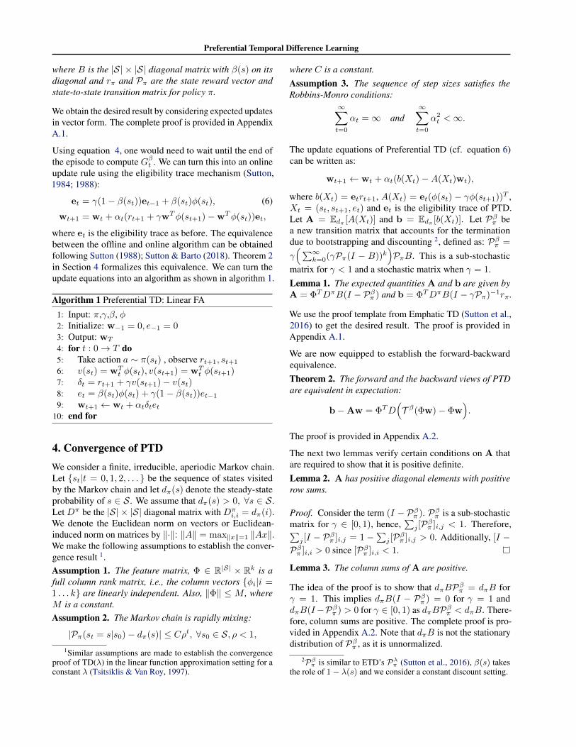
Task description: We consider the 19-state random walkproblem from Sutton 1988; Sutton & Barto 2018. In thisMDP, there are 19 states connected sequentially, with twoterminal states on either side. From each state, the agentcan choose to go left or right. The agent gets a reward of+1 when it transitions to the rightmost terminal state and−1 in the leftmost state; otherwise, rewards are 0. We setγ = 1 and the policy to uniformly random. We compareEmphatic TD, TD(λ), and PTD on this task. We considerfixed parameters for these methods, i.e., interest in ETDis fixed, λ in ETD and TD(λ) are fixed, and β in PTD isfixed. For ETD, we selected a constant interest of 0.01on all states (selected from {0.01, 0.05, 0.1, 0.25} based onhyperparameter search) for each λ-α pair. We consider fixedparameters to understand the differences between the threealgorithms.

Observations: The U-curves obtained are presented in Fig-ure 2, which depicts Root Mean Square Error (RMSE) on

4Code to reproduce the results can be found here.

all states, obtained in the first 10 training episodes, as a func-tion of α. Various curves correspond to different choices offixed λ (or β). In TD(λ), when λ is close to 0, the updatesare close to TD(0), and hence there is high bias. When λ isclose to 1, the updates are close to Monte-Carlo, and there isa high variance. A good bias-variance trade-off is obtainedfor intermediate values of λ, resulting in low RMSE. A simi-lar trade-off can be observed in PTD; however, the trade-offis different from TD(λ). A β value close to 1 results in aTD(0)-style update (similar to λ = 0), but β ≈ 0 results innegligible updates (as opposed to a Monte-Carlo update forsimilar values of λ). The resulting bias-variance trade-off isbetter.

TD(λ) is very sensitive to the value of the learning rate.When λ gets close to 1, the RMSE is high even for a lowlearning rate, resulting in sharp U-curves. This is becauseof the high variance in the updates. However, this is not thecase for PTD, which is relatively stable for all values of βon a wide range of learning rates. PTD exhibits the bestbehaviour when using a learning rate greater than 1 for somevalues of β. This behaviour can be attributed to negligibleupdates performed when a return close to Monte-Carlo (β isclose to 0) is used. Due to negligible updating, the variancein the updates is contained.

The performance of ETD was slightly worse than the othertwo algorithms. ETD is very sensitive to the value of theinterest function. We observed a large drop in performancefor very small changes in the interest value. ETD alsoperforms poorly with low learning rates when the interestis set high. This behaviour can be attributed to the highvariance caused by the emphasis.

6.2. Linear setting

Task description: We consider two toy tasks to evaluatePTD with linear function approximation.

In the first task, depicted in Figure 1a, the agent starts in S1and can pick one of the two available actions, {up, down},transitioning onto the corresponding chain. A goal stateis attached at the end of each chain. Rewards of +2 and−1 are obtained upon reaching the goal state on the upperand lower chains, respectively. The chain has a sequence ofpartially observable states (corridor). In these states, bothactions move the agent towards the goal by one state.

For the second task, we attach two MDPs of the same kindas used in task 1, as shown in Figure 1b. The actions in theconnecting states S1, S2, S3 transition the agent to the up-per and lower chains, but both actions have the same effectin the partially observable states (corridor). A goal state isattached at the end of each chain. To make the task challeng-ing, a stochastic reward (as shown in Figure 1b) is given tothe agent. In both tasks, the connecting states and the goal

https://github.com/NishanthVAnand/Preferential-Temporal-Difference-Learning


0 1 2 3Learning rate

0.20

0.25

0.30

0.35

0.40

0.45

0.50

0.55

0.60

Mea

n R

MSE

ove

r 10

epis

odes

Emphatic TD (interest: 0.01)

0 1 2 3Learning rate

0.20

0.25

0.30

0.35

0.40

0.45

0.50

0.55

0.60

Mea

n R

MSE

ove

r 10

epis

odes

Preferential TD

0.0 0.5 1.0 1.5Learning rate

0.20

0.25

0.30

0.35

0.40

0.45

0.50

0.55

0.60

Mea

n R

MSE

ove

r 10

epis

odes

TD(λ)

0.00.10.20.40.80.90.950.9750.991.0

Figure 2. Root Mean Square Error (RMSE) of Emphatic TD, TD(λ), and Preferential TD as a function of learning rate α. Different curvesin the plot correspond to different values of λ or β (depending upon the algorithm).

states are fully observable and have a unique representation,while the states in the corridor are represented by Gaussiannoise, N (0.5, 1).

0 25 50 75 100Episodes

0.00

0.25

0.50

0.75

1.00

1.25

1.50

1.75

MSE

on

FO s

tate

s

Length = 5

0 25 50 75 100Episodes

0.00

0.25

0.50

0.75

1.00

1.25

1.50

1.75

MSE

on

FO s

tate

s

Length = 15

0 25 50 75 100Episodes

0.00

0.25

0.50

0.75

1.00

1.25

1.50

1.75

MSE

on

FO s

tate

s

Length = 25

ETD variable ETD fixed TD(λ) PTD

(a) Task 1 results

0 50 100 150 200Episodes

0.5

1.0

1.5

2.0

2.5

3.0

3.5

4.0

4.5

MSE

on

FO s

tate

s

Length = 5

0 50 100 150 200Episodes

1.0

1.5

2.0

2.5

3.0

3.5

4.0

4.5

MSE

on

FO s

tate

s

Length = 15

0 50 100 150 200Episodes

1.5

2.0

2.5

3.0

3.5

4.0

4.5

MSE

on

FO s

tate

s

Length = 25

TD(λ) ETD fixed ETD variable PTD

(b) Task 2 results

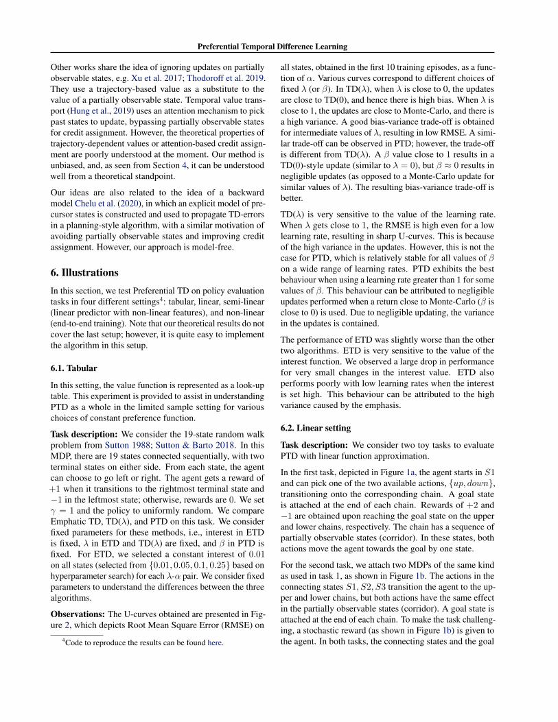
Figure 3. The mean squared error of fully observable states’ valuesplotted as a function of episodes for various algorithms. Differentplots correspond to different lengths of the corridor.

Setup: We tested 4 algorithms: TD(λ), PTD, and two ver-sions of ETD. The first ETD version has a fixed intereston all the states (referred to as ETD-fixed), and the secondvariant has a state-dependent interest (referred to as ETD-variable). We set the preference on fully observable statesto 1 and partially observable states to 0. For a fair com-parison, we make λ a state-dependent quantity by settingthe values of the fully observable states to 0 and 1 on par-tially observable states for TD(λ) and ETD. In the case ofETD-fixed, we set the interest of all states to 0.01 (selectedfrom {0.01, 0.05, 0.1} based on the hyperparameter search,see Appendix A.4.2 for details). For ETD-variable, we setthe interest to 0.5 for fully observable states and 0 on allother states. This choice results in an emphasis of 1 on fully

observable states. ETD-variable yielded very similar perfor-mance with various interest values but with different learn-ing rates. We varied the corridor length ({5, 10, 15, 20, 25})in our experiments. For each length and algorithm, we chosean optimal learning rate from 20 different values. We usedγ = 1, a uniformly random policy, and the value functionis predicted only at fully observable states. The results areaveraged across 25 seeds, and a confidence interval of 95%is used in the plots5.

Observations: A state-dependent λ (or β) results in boot-strapping from fully observable states only. Additionally,PTD weighs the updates on various states according to β.The learning curves on both tasks are reported in Figures3 and A.2. TD(λ) performs poorly, and the errors increasewith the length of the chain on both tasks. Also, the values ofthe fully observable states stop improving even as the num-ber of training episodes increases. This is to be expected, asTD(λ) updates the values of all states. Thus, errors in esti-mating the partially observable states affect the predictionsat the fully observable states due to the generalization in thefunction approximator.

ETD-fixed performs a very small update on partially observ-able states due to the presence of a small interest. Never-theless, this is sufficient to affect the predictions on fullyobservable states. The error in ETD-fixed increases witha small increase in the interest. ETD-fixed is also highlysensitive to the learning rate. However, ETD-variable per-forms the best. With the choice of λ and interest functiondescribed previously, ETD-variable ignores the updates oncorridor states and, at the same time, does not bootstrapfrom these states, producing a very low error in both tasks.This effect is similar to PTD. However, bootstrapping andupdating are controlled by a single parameter (β) in PTD,while ETD-variable has two parameters, λ and the interestfunction, and we have to optimize both. Hence, while it

5We use the t-distribution to compute the confidence intervalsin all the settings.


converges slightly faster than PTD, this is at the cost ofincreased tuning complexity.

6.3. Semi-linear setting

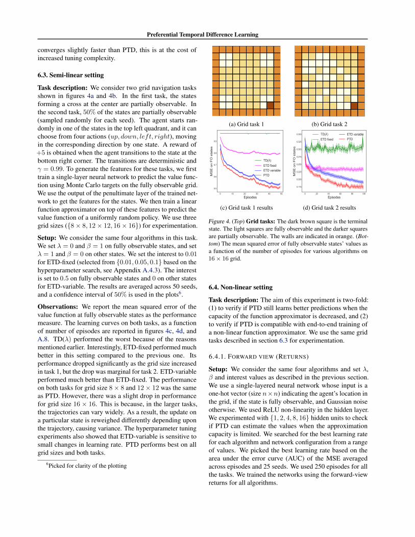
Task description: We consider two grid navigation tasksshown in figures 4a and 4b. In the first task, the statesforming a cross at the center are partially observable. Inthe second task, 50% of the states are partially observable(sampled randomly for each seed). The agent starts ran-domly in one of the states in the top left quadrant, and it canchoose from four actions (up, down, left, right), movingin the corresponding direction by one state. A reward of+5 is obtained when the agent transitions to the state at thebottom right corner. The transitions are deterministic andγ = 0.99. To generate the features for these tasks, we firsttrain a single-layer neural network to predict the value func-tion using Monte Carlo targets on the fully observable grid.We use the output of the penultimate layer of the trained net-work to get the features for the states. We then train a linearfunction approximator on top of these features to predict thevalue function of a uniformly random policy. We use threegrid sizes ({8× 8, 12× 12, 16× 16}) for experimentation.

Setup: We consider the same four algorithms in this task.We set λ = 0 and β = 1 on fully observable states, and setλ = 1 and β = 0 on other states. We set the interest to 0.01for ETD-fixed (selected from {0.01, 0.05, 0.1} based on thehyperparameter search, see Appendix A.4.3). The interestis set to 0.5 on fully observable states and 0 on other statesfor ETD-variable. The results are averaged across 50 seeds,and a confidence interval of 50% is used in the plots6.

Observations: We report the mean squared error of thevalue function at fully observable states as the performancemeasure. The learning curves on both tasks, as a functionof number of episodes are reported in figures 4c, 4d, andA.8. TD(λ) performed the worst because of the reasonsmentioned earlier. Interestingly, ETD-fixed performed muchbetter in this setting compared to the previous one. Itsperformance dropped significantly as the grid size increasedin task 1, but the drop was marginal for task 2. ETD-variableperformed much better than ETD-fixed. The performanceon both tasks for grid size 8× 8 and 12× 12 was the sameas PTD. However, there was a slight drop in performancefor grid size 16 × 16. This is because, in the larger tasks,the trajectories can vary widely. As a result, the update ona particular state is reweighed differently depending uponthe trajectory, causing variance. The hyperparameter tuningexperiments also showed that ETD-variable is sensitive tosmall changes in learning rate. PTD performs best on allgrid sizes and both tasks.

6Picked for clarity of the plotting

(a) Grid task 1 (b) Grid task 2

0 10 20 30 40 50

Episodes

0.5

0.6

0.7

0.8

0.9

MS

E o

n F

O s

tate

s

TD(λ)ETD fixedETD variablePTD

(c) Grid task 1 results

0 20 40 60 80 100

Episodes

0.175

0.200

0.225

0.250

0.275

0.300

0.325

0.350

MS

E o

n F

O s

tate

s

TD(λ)ETD fixed

ETD variablePTD

(d) Grid task 2 results

Figure 4. (Top) Grid tasks: The dark brown square is the terminalstate. The light squares are fully observable and the darker squaresare partially observable. The walls are indicated in orange. (Bot-tom) The mean squared error of fully observable states’ values asa function of the number of episodes for various algorithms on16× 16 grid.

6.4. Non-linear setting

Task description: The aim of this experiment is two-fold:(1) to verify if PTD still learns better predictions when thecapacity of the function approximator is decreased, and (2)to verify if PTD is compatible with end-to-end training ofa non-linear function approximator. We use the same gridtasks described in section 6.3 for experimentation.

6.4.1. FORWARD VIEW (RETURNS)

Setup: We consider the same four algorithms and set λ,β and interest values as described in the previous section.We use a single-layered neural network whose input is aone-hot vector (size n×n) indicating the agent’s location inthe grid, if the state is fully observable, and Gaussian noiseotherwise. We used ReLU non-linearity in the hidden layer.We experimented with {1, 2, 4, 8, 16} hidden units to checkif PTD can estimate the values when the approximationcapacity is limited. We searched for the best learning ratefor each algorithm and network configuration from a rangeof values. We picked the best learning rate based on thearea under the error curve (AUC) of the MSE averagedacross episodes and 25 seeds. We used 250 episodes for allthe tasks. We trained the networks using the forward-viewreturns for all algorithms.


1 2 4 8 16Number of hidden units

0.5

1.0

1.5

2.0

2.5

AUC

of M

ean

erro

r

Grid size = 8


0.4

0.6

0.8

1.0

1.2

1.4

AUC

of M

ean

erro

r

Grid size = 12


0.3

0.4

0.5

0.6

0.7

0.8

0.9

1.0

AUC

of M

ean

erro

r

Grid size = 16

PTDTD(λ)ETD fixedETD variable

(a) Grid task 1 results


0.2

0.3

0.4

0.5

0.6

AUC

of a

vera

ged

MSE

Grid size = 8


0.15

0.20

0.25

0.30

0.35

0.40

AUC

of a

vera

ged

MSE

Grid size = 12


0.08

0.10

0.12

0.14

0.16

0.18

0.20

0.22

0.24

AUC

of a

vera

ged

MSE

Grid size = 16TD(λ)ETD fixedETD variablePTD

(b) Grid task 2 results

Figure 5. The area under the curve (AUC) of mean squared error ofthe values of the fully observable states, averaged across seeds andepisodes as a function of the number of hidden units for variousalgorithms. The error bars indicate the confidence interval of 90%across 50 seeds. Different plots corresponds to different sizes ofthe grid task.

Observations: The results are presented in Figure 5. Eachpoint in the plot is the AUC of the MSE for an algorithm andneural network configuration pair averaged across episodesand seeds. The error bars indicate the confidence interval of90% across seeds. TD(λ) performs poorly because of thereasons stated before. ETD-fixed performs slightly betterthan TD(λ), but the error is still high. PTD performs betterthan the other algorithms on both tasks and across all net-work sizes. The error is high only in the 16 × 16 grid forreally small networks, with four or fewer hidden units. Thisis because the number of fully observable states is signifi-cantly larger for this grid size, and the network is simply notlarge enough to provide a good approximation for all thesestates. Nevertheless, PTD’s predictions are significantlybetter than other algorithms in this setting. The behaviorof ETD-variable is similar, but the variance is much higher.As before, hyperparameter tuning experiments indicate thatETD is also much more sensitive to learning rates.

6.4.2. BACKWARD VIEW (ELIGIBILITY TRACES)

In this experiment, we are interested in finding out howPTD’s eligibility traces would fare in the non-linear setting.

Setup: The set of algorithms tested, network architecture,and the task details are same as Section 6.4.1. We alsofollowed the same procedure as the previous section toselect the learning rate. We trained the networks in anonline fashion using eligibility traces for all algorithms.

Observations: Eligibility traces facilitate online learning,


0.4

0.6

0.8

1.0

1.2

1.4

1.6

1.8

AUC

of M

ean

erro

r

Grid size = 8


0.4

0.6

0.8

1.0

1.2

1.4

AUC

of M

ean

erro

r

Grid size = 12


0.3

0.4

0.5

0.6

0.7

0.8

0.9

AUC

of M

ean

erro

r

Grid size = 16

PTDTD(λ)ETD fixedETD variablePTD (forward)

(a) Grid task 1 results


0.15

0.20

0.25

0.30

0.35

0.40

0.45

0.50

0.55

AUC

of M

ean

erro

r

Grid size = 8


0.125

0.150

0.175

0.200

0.225

0.250

0.275

0.300

0.325

AUC

of M

ean

erro

r

Grid size = 12


0.08

0.10

0.12

0.14

0.16

0.18

0.20

0.22

0.24

AUC

of M

ean

erro

r

Grid size = 16PTDTD(λ)ETD fixedETD variablePTD (forward)

(b) Grid task 2 results

Figure 6. The area under the curve (AUC) of mean squared error ofthe values of the fully observable states, averaged across seeds andepisodes as a function of the number of hidden units for variousalgorithms. The error bars indicate the confidence interval of 90%across 50 seeds. Different plots corresponds to different sizes ofthe grid task.

and they provide a way to assign credit to the past states,making it a valuable tool in theory. However, the predictionerrors of all the algorithms are higher than their forwardview counterparts. The drop in performance is because eli-gibility traces remember the gradient that is computed withrespect to the past parameters, which introduces significantbias. Besides, the bias in the eligibility traces caused insta-bilities in the training procedure of PTD and ETD-variablefor high learning rates. The results are presented in Figure6. As shown, the performances of TD(λ) and ETD-fixedperforms are still poor compared to PTD and ETD-variable.Backward views of PTD and ETD-variable have slightlymore error and variance across the seeds than their forwardview equivalents when the capacity of the function approx-imator is small. However, they match the forward viewperformance when the capacity is increased. PTD still per-forms slightly better than ETD-variable in the 16× 16 grids,indicating the usefulness of its eligibility traces with neuralnetworks.

7. Conclusions and Future WorkWe introduced Preferential TD learning, a novel TD learningmethod that updates the value function and bootstraps in thepresence of state-dependent preferences, which allow theseoperations to be prioritized differently in different states.Our experiments show that PTD compares favourably toother TD variants, especially on tasks with partial observ-ability. However, partial observability is not a requirement


to use our method. PTD can be useful in other settingswhere updates can benefit from re-weighting. For instance,in an environment with bottleneck states, having a highpreference on such states could propagate credit faster. Pre-liminary experiments in Appendix A.4.5 corroborate thisclaim, and further analysis could be interesting.

We set the preference function from the beginning to afixed value in our experiments, but an important directionfor future work is to learn or adapt it based on data. Thepreference function plays a dual role: its presence in thetargets controls the amount of bootstrapping from futurestate values, and its presence in the updates determinesthe amount of re-weighting. Both can inspire learning ap-proaches. The bootstrapping view opens the door to existingtechniques such as meta-learning (White & White, 2016; Xuet al., 2018; Zhao et al., 2020), variance reduction (Kearns& Singh, 2000; Downey et al., 2010), and gradient interfer-ence (Bengio et al., 2020). Alternatively, we can leveragemethods that identify partially observable states or importantstates (e.g. bottleneck states) (McGovern & Barto, 2001;Stolle & Precup, 2002; Bacon et al., 2017; Harutyunyanet al., 2019) to learn the preference function. We also be-lieve that PTD would be useful in transfer learning, whereone could learn parameterized preferences in a source taskand use them in the updates on a target task to achieve fastertraining.

We demonstrated the utility of preferential updating in on-policy policy evaluation. The idea of preferential updatingcould also be exploited in other RL settings, such as off-policy learning, control, or policy gradients, to achieve fasterlearning. Our algorithm could also be applied to learningGeneral Value Functions (Comanici et al., 2018; Suttonet al., 2011), an exciting future direction.

As discussed earlier, our method bridges the gap betweenEmphatic TD and TD(λ). Eligibility traces in PTD propa-gate the credit to the current state based on its preference,and the remaining credit goes to the past states. This idea issimilar to the gradient updating scheme in the backpropa-gation through time algorithm, where the gates in recurrentneural networks control the flow of credit to past states. Wesuspect an interesting connection between the eligibilitytrace mechanism in PTD and backpropagation through time.In the binary preference setting (β ∈ {0, 1}), our methodcompletely discards zero preference states in the MDP frombootstrapping and updating. The remaining states, whosepreference is non-zero, participate in both. This creates alevel of state abstraction in the given problem.

Our ultimate goal is to train a small agent capable of learn-ing in a large environment, where the agent can’t representvalues correctly everywhere since the state space is enor-mous (Silver et al., 2021). A logical step towards this goal isto find ways to effectively use function approximators with

limited capacity compared to the environment. Therefore, itshould prefer to update and bootstrap from a few states wellrather than poorly estimate the values for all states. PTDhelps achieve this goal and opens up avenues for developingmore algorithms of this flavour.

AcknowledgementsThis research was funded through grants from NSERC andthe CIFAR Learning in Machines and Brains Program. Wethank Ahmed Touati for the helpful discussions on theory;and the anonymous reviewers and several colleagues at Milafor the constructive feedback on the draft.

ReferencesAberdeen, D. Filtered reinforcement learning. In European

Conference on Machine Learning, pp. 27–38. Springer,2004.

Bacon, P.-L., Harb, J., and Precup, D. The option-criticarchitecture. In Proceedings of the AAAI Conference onArtificial Intelligence, volume 31/1, 2017.

Barnard, E. Temporal-difference methods and markov mod-els. IEEE Transactions on Systems, Man, and Cybernet-ics, 23(2):357–365, 1993.

Bengio, E., Pineau, J., and Precup, D. Interference andgeneralization in temporal difference learning. In Inter-national Conference on Machine Learning, pp. 767–777.PMLR, 2020.

Bertsekas, D. P. and Tsitsiklis, J. N. Neuro-dynamic pro-gramming. Athena Scientific, 1996.

Brockman, G., Cheung, V., Pettersson, L., Schneider, J.,Schulman, J., Tang, J., and Zaremba, W. Openai gym.arXiv preprint arXiv:1606.01540, 2016.

Chelu, V., Precup, D., and van Hasselt, H. Forethoughtand hindsight in credit assignment. Advances in NeuralInformation Processing Systems (NeurIPS), 2020.

Comanici, G., Precup, D., Barreto, A., Toyama, D. K.,Aygun, E., Hamel, P., Vezhnevets, S., Hou, S., andMourad, S. Knowledge representation for reinforcementlearning using general value functions. Open review,2018.

Downey, C., Sanner, S., et al. Temporal difference bayesianmodel averaging: A bayesian perspective on adaptinglambda. In ICML, pp. 311–318. Citeseer, 2010.

Ghiassian, S., Rafiee, B., and Sutton, R. S. A first empiricalstudy of emphatic temporal difference learning. arXivpreprint arXiv:1705.04185, 2017.


Gordon, G. J. Chattering in SARSA(λ). A CMU learninglab internal report. Citeseer, 1996.

Harutyunyan, A., Dabney, W., Mesnard, T., Azar, M. G.,Piot, B., Heess, N., van Hasselt, H. P., Wayne, G., Singh,S., Precup, D., et al. Hindsight credit assignment. InAdvances in neural information processing systems, pp.12467–12476, 2019.

Hung, C.-C., Lillicrap, T., Abramson, J., Wu, Y., Mirza,M., Carnevale, F., Ahuja, A., and Wayne, G. Optimizingagent behavior over long time scales by transporting value.Nature communications, 10(1):1–12, 2019.

Kearns, M. J. and Singh, S. P. Bias-variance error boundsfor temporal difference updates. In COLT, pp. 142–147.Citeseer, 2000.

Loch, J. and Singh, S. P. Using eligibility traces to find thebest memoryless policy in partially observable markovdecision processes. In ICML, pp. 323–331, 1998.

Mahmood, A. Incremental off-policy reinforcement learn-ing algorithms. Ph.D. thesis, U of Alberta, 2017.

McGovern, A. and Barto, A. G. Automatic discovery of sub-goals in reinforcement learning using diverse density. InProceedings of the Eighteenth International Conferenceon Machine Learning, ICML ’01, pp. 361–368, San Fran-cisco, CA, USA, 2001. Morgan Kaufmann Publishers Inc.ISBN 1558607781.

Mnih, V., Kavukcuoglu, K., Silver, D., Rusu, A. A., Veness,J., Bellemare, M. G., Graves, A., Riedmiller, M., Fidje-land, A. K., Ostrovski, G., et al. Human-level controlthrough deep reinforcement learning. Nature, 518(7540):529–533, 2015.

Schulman, J., Wolski, F., Dhariwal, P., Radford, A., andKlimov, O. Proximal policy optimization algorithms.CoRR, abs/1707.06347, 2017.

Seijen, H. and Sutton, R. True online td (lambda). InInternational Conference on Machine Learning, pp. 692–700, 2014.

Silver, D., Singh, S., Precup, D., and Sutton, R. S. Rewardis enough. Artificial Intelligence, pp. 103535, 2021.

Singh, S. P. and Sutton, R. S. Reinforcement learning withreplacing eligibility traces. Machine learning, 22(1-3):123–158, 1996.

Stolle, M. and Precup, D. Learning options in reinforcementlearning. In International Symposium on abstraction,reformulation, and approximation, pp. 212–223. Springer,2002.

Sutton, R. S. Temporal credit assignment in reinforcementlearning, phd thesis. University of Massachusetts, De-partment of Computer and Information Science, 1984.

Sutton, R. S. Learning to predict by the methods of temporaldifferences. Machine learning, 3(1):9–44, 1988.

Sutton, R. S. Td models: Modeling the world at a mixtureof time scales. In Machine Learning Proceedings 1995,pp. 531–539. Elsevier, 1995.

Sutton, R. S. and Barto, A. G. Reinforcement learning: Anintroduction. MIT press, 2018.

Sutton, R. S., Precup, D., and Singh, S. Between mdpsand semi-mdps: A framework for temporal abstraction inreinforcement learning. Artificial intelligence, 112(1-2):181–211, 1999.

Sutton, R. S., Modayil, J., Delp, M., Degris, T., Pilarski,P. M., White, A., and Precup, D. Horde: A scalablereal-time architecture for learning knowledge from unsu-pervised sensorimotor interaction. In The 10th Interna-tional Conference on Autonomous Agents and MultiagentSystems - Volume 2, AAMAS ’11, pp. 761–768, Rich-land, SC, 2011. International Foundation for AutonomousAgents and Multiagent Systems. ISBN 0982657161.

Sutton, R. S., Mahmood, A. R., and White, M. An emphaticapproach to the problem of off-policy temporal-differencelearning. The Journal of Machine Learning Research, 17(1):2603–2631, 2016.

Theocharous, G. and Kaelbling, L. P. Approximate planningin pomdps with macro-actions. In Advances in NeuralInformation Processing Systems, pp. 775–782, 2004.

Thodoroff, P., Anand, N., Caccia, L., Precup, D., and Pineau,J. Recurrent value functions. 4th Multidisciplinary Con-ference on Reinforcement Learning and Decision Making(RLDM), 2019.

Tsitsiklis, J. N. and Van Roy, B. An analysis of temporal-difference learning with function approximation. IEEEtransactions on automatic control, 42(5):674–690, 1997.

van Hasselt, H. and Sutton, R. S. Learning to predict in-dependent of span. arXiv preprint arXiv:1508.04582,2015.

Varga, R. S. Matrix iterative analysis, volume 27. SpringerScience & Business Media, 1999.

Watkins, C. J. C. H. Learning from delayed rewards. King’sCollege, Cambridge, 1989.

White, M. and White, A. A greedy approach to adaptingthe trace parameter for temporal difference learning. In


Proceedings of the 2016 International Conference on Au-tonomous Agents and Multiagent Systems, AAMAS ’16,pp. 557–565, Richland, SC, 2016. InternationalFounda-tion for Autonomous Agents and Multiagent Systems.ISBN 9781450342391.

Xu, Z., Modayil, J., van Hasselt, H. P., Barreto, A., Silver,D., and Schaul, T. Natural value approximators: Learningwhen to trust past estimates. In Advances in NeuralInformation processing systems, pp. 2120–2128, 2017.

Xu, Z., van Hasselt, H. P., and Silver, D. Meta-gradient re-inforcement learning. In Advances in neural informationprocessing systems, pp. 2396–2407, 2018.

Yu, H. On convergence of emphatic temporal-differencelearning. In Conference on Learning Theory, pp. 1724–1751, 2015.

Yu, H., Mahmood, A. R., and Sutton, R. S. On generalizedbellman equations and temporal-difference learning. TheJournal of Machine Learning Research, 19(1):1864–1912,2018.

Zhao, M., Luan, S., Porada, I., Chang, X.-W., and Pre-cup, D. Meta-learning state-based eligibility tracesfor more sample-efficient policy evaluation. In In-ternational Conference on Autonomous Agents andMultiagent Systems, AAMAS ’20. International Foun-dation for Autonomous Agents and Multiagent Sys-tems, 2020. URL http://www.ifaamas.org/Proceedings/aamas2020/pdfs/p1647.pdf.

http://www.ifaamas.org/Proceedings/aamas2020/pdfs/p1647.pdf

http://www.ifaamas.org/Proceedings/aamas2020/pdfs/p1647.pdf

Preferential Temporal Difference Learning

Documents

Transcript of Preferential Temporal Difference Learning