ISSN 1471-0498

DEPARTMENT OF ECONOMICS

DISCUSSION PAPER SERIES

PREFERENCES OVER LEISURE AND CONSUMPTION OF SIBLINGS AND INTRA-HOUSEHOLD ALLOCATION

Martina Kirchberger

Number 713 July 2014

Manor Road Building, Manor Road, Oxford OX1 3UQ

PREFERENCES OVER LEISURE AND CONSUMPTION

OF SIBLINGS AND INTRA-HOUSEHOLD ALLOCATION

Martina KIRCHBERGERa∗

a Centre for the Study of African Economies,

Department of Economics, University of Oxford

1 July 2014

ABSTRACT

Children are increasingly treated as active members in the household. However, their preferences

over consumption and leisure are rarely modelled. This paper considers heterogeneity in siblings’

preferences over leisure and consumption and builds a theoretical and empirical model for chil-

dren’s time and consumption allocations in a household. We test the predictions of the model with

unique data from Ethiopia, India, Peru and Vietnam which contain detailed information on time

use and allocations of assignable goods for sibling pairs. We find that conditioning on observable

variables, the residuals of these simultaneous decisions are significantly negatively correlated.

This suggests that differences in siblings’ relative time and consumption allocations are driven by

their relative preferences over leisure and consumption rather than differences in parents’ relative

altruism. Families seem to function as market economies in which children trade off leisure and

consumption, select their optimal bundle, and are rewarded by their parents accordingly.

Keywords: Intra-household allocation, children.

JEL Classification: D1, J1, J2.

∗I would like to express my sincere gratitude to Martin Browning and Stefan Dercon for their support, generous time, and manyhelpful discussions. I am also grateful to Orazio Attanasio, Steve Bond, Pierre-André Chiappori, Matt Collin, Cheryl Doss, Mikhail Drugov,Eric Edmonds, Marcel Fafchamps, Michael Keane, Sonya Krutikova, Clare Leaver, Erzo Luttmer, Marta Troya Martinez, Aureo de Paula,Simon Quinn, Francis Teal, Gerhard Toews, Chris Udry, Frederic Vermeulen, Jeffrey Wooldridge, Andrew Zeitlin and participants at theEconometric Society European Meetings 2013, the Conference on Inequalities in Children’s Outcomes in Developing Countries 2013,the Development Economics Conference of the German Economic Association 2013, the Royal Economic Society Annual Conference,the NEUDC Conference 2012, the CSAE Conference 2012, Spring Meeting of Young Economists 2012, the Gorman Workshop and theCSAE workshop at Oxford for helpful comments and discussions. I acknowledge Young Lives for providing the household data for thepurpose of this research. Young Lives is an international study of childhood poverty, following the lives of 12,000 children in 4 countries(Ethiopia, India, Peru and Vietnam) over 15 years. www.younglives.org.uk. Young Lives is core-funded from 2001 to 2017 by UK aidfrom the Department for International Development (DFID), and co-funded by the Netherlands Ministry of Foreign Affairs from 2010 to2014. Sub-studies are funded by the Bernard van Leer Foundation and the Oak Foundation. The views expressed are those of the author.They are not necessarily those of, or endorsed by, Young Lives, the University of Oxford, DFID or other funders. I am grateful for fundingfrom the AXA Research Fund. All errors are my own. Correspondence: Centre for the Study of African Economies (CSAE), Departmentof Economics, Manor Road Building, Oxford OX1 3UQ, UK; Email: martina.kirchberger@economics.ox.ac.uk.

1

1 Introduction

Economists increasingly consider children as active members in the household1 who affect

household expenditure allocations (Moehling 2005; Lundberg et al. 2009; Kapan 2009;

Dauphin et al. 2010) and their own time allocations (Berry 2013; Bursztyn and Coffman

2012; Kremer et al. 2009). Recent evidence from lab experiments highlights heterogeneity

in children’s risk taking, attitudes towards ambiguity, time preferences, and competitiveness

(Castillo et al. 2011; Andersen et al. 2013; Sutter et al. 2013)2. Most parents will also

agree that children growing up in the same household can be very different in their per-

sonality traits and preferences (Daniels and Plomin 1985; Dunn and Plomin 1990)3. Still,

economic models traditionally do not take into account heterogeneity in children’s pref-

erences within families and how these shape consumption and leisure allocations. When

considering children as economic agents with preferences over consumption and leisure,

it becomes natural to employ standard models employed in the labor economics literature

in which agents maximize utility from consumption and leisure subject to a budget con-

straint. The objective of this paper is to understand whether children’s preferences over

consumption and leisure determine allocations of consumption and leisure among siblings.

The central contribution of the paper is twofold. First, it develops a unitary model of

the household focusing on the role of heterogeneity in preferences of children and intra-

sibling allocation of consumption and leisure4. The model assumes parents to be social

planners taking into account children’s preferences over leisure and consumption when

making allocation decisions. The paper focuses on how allocations are driven conditional

on children being in school rather than the tradeoff between work and school, so we ab-

stract from schooling decisions5. The model provides insights into how heterogeneity in

1The psychology literature has long recognized the role of children in household decision making andstudies on child development suggest a process of gradual increase of shared decision making towards decisionautonomy from childhood into adolescence (Grotevant 1983; Dornbusch et al. 1985; Yee and Flanagan1985). Harbaugh et al. (2003) play dictator and ultimatum games with children and find that they are goodbargainers by the age of 7, in the sense that they are aware of their own and their partner’s pay-offs in a specificsituation. Evidence from an experiment conducted by Harbaugh et al. (2001) suggests that by the age of 11,children’s choices are roughly as rational as choices by adults, so that their choices satisfy the GeneralizedAxiom of Revealed Preference. Choices made by about 60% of 11 year old children and undergraduates areconsistent with utility maximization, compared to about 25% of 7 year old children. Lundberg et al. (2009)show that there is a sharp increase in children’s reported involvement in the decision making process betweenage 10-14.

2Castillo et al. (2011) and Sutter et al. (2013) show how differences in preferences elicited in experimentssignificantly correlate with differences in observed behaviors in real life, such as school referrals, smoking,alcohol consumption and saving of pupils in Georgia (United States) and Tyrol (Austria). Orkin (2011)presents qualitative evidence from children in rural Ethiopia supporting the idea that even within one villagechildren have different preferences with regard to work as well as make decisions regarding their time.

3One of the earliest studies documenting the low correlation of personality inventories between siblingswas Crook (1937) using the Bernreuter personality inventory.

4Our approach is most closely related to Browning and Gørtz (2012) who model the allocation of con-sumption and leisure between husband and wife.

5Our model therefore does not view child work and schooling as substitutes, which is in line with evidencefound by Attanasio et al. (2010). They show that increases in schooling hours caused by the Familias en

2

children’s preferences and parental altruism affect allocations and yields testable proposi-

tions. The intuition is straightforward. Assume there is a family with two children, child

A and child B, who face equal pay. If relative parental altruism towards child A and B

drives allocation decisions and children’s relative preferences over leisure and consump-

tion are independently distributed, we expect relative expenditure and relative leisure to

be positively correlated, controlling for observable exogenous characteristics. The favorite

child gets allocated a higher expenditure share and higher leisure share. On the other

hand, if relative preferences over leisure and consumption drive allocations, relative pref-

erences for leisure and consumption are negatively correlated, and there is no variation in

parental altruism, controlling for observable exogenous characteristics, relative leisure and

relative consumption should be negatively correlated. Children who work longer hours get

rewarded accordingly6.

Second, we use detailed data on time use and assignable goods of a panel data set

of children in Ethiopia, India, Peru and Vietnam to test the theoretical implications of the

model. Data on both time use of children in the household and assignable expenditures

from household surveys is rare for adults (Browning and Gørtz 2012), and even more so

for children. We use data on the amount of time children spend on leisure and work activ-

ities, and child-specific clothes expenditures. To our knowledge, this is the first paper that

explicitly models within sibling variation in preferences over leisure and consumption and

tests the predictions of the theoretical model with a data set of children who are in full time

schooling and haven’t entered the formal labor market yet in the context of four developing

countries.

We find that conditioning on observable variables, relative leisure and relative consump-

tion are significantly negatively correlated. This suggests that differences in siblings’ relative

time and consumption allocations are driven by their relative preferences over leisure and

consumption rather than differences in the relative altruism of parents vis-à-vis their chil-

dren. This correlation is robust to excluding younger children and non-biological siblings.

When we use a different measure of relative time allocation, relative work hours instead

of relative leisure, we find further evidence consistent with the hypothesis that preferences

are driving allocations rather than altruism toward a particular child. We also show that

this finding persists when we only explore variation in the hours worked in the household,

ruling out that the positive correlation between relative work and relative expenditure is

due to children working outside the house and therefore needing more work-related clothes

expenditures. Finally, we do not find evidence that the relationship is driven by age-gender-

location specific productivity differences, non-linear age effects, different levels of educa-

tion and schooling hours, and a range of alternative hypotheses. Children seem to trade off

Acción program in Colombia did not map one to one into reductions in work hours; rather, the results suggestthat leisure time of children decreased.

6These are the extreme cases. In reality, both relative altruism and relative preferences might play a rolein determining allocations. The empirical analysis allows us to examine which of the two dominates.

3

leisure and consumption and are rewarded accordingly. As a result, the data is consistent

with a model in which families behave as if they were an internal market in which children

select their optimal consumption-leisure bundle.

This is important for two at least two reasons. First, the model shows that if siblings

have different preferences over leisure and consumption, it is efficient for parents to take

these into account when making allocations in the household. Parents might possess infor-

mation on preference heterogeneity among their children not available to policy makers.

An implication is that blanket policies might be welfare reducing as they prohibit parents to

take into account children’s preferences over leisure and consumption. Further, we abstract

the focus from the schooling-child labor trade-off traditionally employed in the literature,

as we only look at children who are in full time schooling. The fact that we find hetero-

geneity in children’s leisure and work allocations despite their full time enrolment status

suggests that there are other factors that affect their time allocation apart from schooling7.

The approach adopted in this paper is based on the assumption that household allo-

cations are efficient, an assumption embodied in unitary as well as collective household

models, which explicitly assume the existence of an efficient intra-household decision mak-

ing process (Becker 1981; Chiappori 1988; Browning and Chiappori 1998). Among the first

to explicitly consider parent-children interactions was Becker (1981) with his well known

Rotten Kid Theorem. Within the literature on intra-household allocations, the presence of

children and their effect on household economic behavior has received increasing atten-

tion over the past 20 years (Browning 1992; Browning and Lechene 2003; Browning and

Ejrnæs 2009; Bonke and Browning 2011; Blundell et al. 2005; Cherchye et al. 2012).

A recent paper by Dunbar et al. (2013) uses semi-parametric restrictions to identify the

resource shares in a household allocated to children with the goal of estimating children’s

poverty levels in Malawi. The data employed in this chapter allows us to investigate how

child-specific expenditures relate to children’s time allocations.

Our focus on within sibling allocation of resources by parents also relates to the liter-

ature on child quantity and quality trade-offs, parental investment, and parental prefer-

ences for equality among their children. Becker and Lewis (1973) highlight the interaction

between the quantity and quality of children: a larger number of children increases the

marginal cost of quality, and vice versa. Becker and Tomes (1976) show that when chil-

dren have different endowments, and the return to human capital investment is higher for

high-endowment children, parents exacerbate these differences by investing human capital

more heavily in the child with the higher endowments8. Whether parents reinforce or com-

7Empirically we are not able to distinguish whether our findings are generated by children’s primitive orderived preferences; in other words, whether the observed behavior is due to children’s intrinsic preferencesor a reaction to incentives offered by parents; what is important is that both implications remain valid ineither case.

8Behrman et al. (1995) highlight that this finding requires equal concern of parents, sufficiently high levelsof resources allocated to children, and higher marginal as well as average returns to education for the moreable child.

4

pensate endowments is still an open question in the literature9. Our paper differs from this

literature in that we focus on a consumption good (clothes) rather than investment goods

(i.e. education, health) and abstract from differences in initial endowments of children10.

In our model, inequality in leisure and consumption among siblings can be due to differ-

ences in parental preferences as well as differences in children’s preferences over leisure

and consumption11. Finally, we do not explore the effect of family size due to limitations

in the data: as we are able to identify expenditure shares and leisure time only for children

with one other sibling in the age range of 5-17, we limit our sample to families with two

children in this age group without younger siblings.

A few studies have departed from modeling children via caring preferences or as a

household public good to consider them as agents in the household. Moehling (2005)

shows that adolescents’ labor force participation is positively correlated with their clothing

expenditures using data from the Cost of Living Survey of 1917-1919 in the United States.

Dustmann and Micklewright (2001) use data from sixteen year old adolescents from the

British National Child Development Study and find that adolescents’ labor force participa-

tion reduces parental transfers12. This focus of this paper differs from these studies in that

we are interested in how relative preferences of siblings and relative altruism of parents

affect relative expenditures between siblings.

Dauphin et al. (2010) examine the demand systems of families with one child aged

sixteen and over living with his or her parents using data from the United Kingdom; they

find that the data are consistent with three decision makers for the complete sample, the

sample of children aged 16-21 and for daughters (irrespective of their age). Kapan (2009)

uses data from Turkey and finds that while the unitary model is not rejected for families

in which the wife does not earn an income, it is strongly rejected when a son aged 12 and

above is present in the household (but not for daughters). Instead of examining proper-

ties of demand systems to test whether the data are consistent with more decision makers

when older children are present, our approach is to develop a model which delivers testable

propositions on relative preferences and relative expenditures of siblings. Finally, this paper

also relates to the literature on child labor. Edmonds (2008)[p. 3668] points out that “fu-

9There is evidence for compensatory behavior of parents (Behrman et al. 1982; Griliches 1979), as well asreinforcement (Behrman et al. 1994; Rosenzweig and Zhang 2009). Parents might also be both reinforcingand compensating differences in different dimensions. Conti et al. (2010) use data from Chinese twins andfind that parents make compensating investments in health and reinforcing investments in education, andthere is no effect on the time parents spend with children. Barcellos et al. (2014) find that parents treat boysfavorably in almost every dimension of child investment in India.

10Ideally we would like to test for the role of ability as well; unfortunately, our data only contains informa-tion of ability for the panel child but not the siblings.

11We do not make assumptions over what determines heterogeneity in parental altruism towards theirchildren.

12Moehling (2005) argues that during the time of their data income of children entered the householdbudget so that it increased the bargaining power of children, while Dustmann and Micklewright (2001) arguethat for their sample earnings of adolescents remain directly in the hands of the adolescent, so that parentsrespond by reducing transfers.

5

ture research understanding the child’s own role in her time allocation is perhaps the most

pressing need in the child labor literature”. If children have agency over their decisions even

in relatively poor settings, considering their preferences is instrumental to understanding

households’ behavior in low income countries.

The paper is structured as follows: section 2 presents the context and data. Section

3 develops a theoretical model. Section 4 focuses on identification and estimation of the

model parameters. Section 5 discusses the results and section 6 concludes.

2 Data

Detailed data on allocations of time and goods within families is very rare. In the majority

of household surveys we observe total household expenditures for particular goods, where

at most it is possible to assign a few goods to husband, wife and children after making

assumptions about the characteristics of goods. Detailed data on time allocations across

household members is even sparser. Having both pieces of information in the same survey

is crucial for studying their interaction. We use data from the Young Lives Survey, a study

of childhood poverty tracking two cohorts of children in Ethiopia, India, Peru and Vietnam.

For the purpose of this paper, we use data from the older cohort which is 7-8 years old

when first interviewed in 2002. The second and third rounds took place in 2006/2007 and

2009/2010 and collected detailed information on expenditures as well as information on

what activities all household members aged 5-17 spent time on during a usual workday.

The survey contains one ’panel’ or ’index’ child per family (which determines the panel

dimension of the survey), but also collects detailed information on other family members in

the household. Focusing on a cohort over time has the advantage that we can inspect how

a relatively homogenous sample of children at two points of time interacts with siblings.

From the whole data set we select our sample along four dimension: (i) as we can assign

expenditures with certainty only to children with one other sibling, we use the sample of

children with one other child below 18 years old in the household; (ii) since the time diary

is available only for children between 5 and 17, we limit the sample to panel children with

siblings between 5 and 17 years; (iii) given that we are interested in time allocations for

children who are in school, we raise the age cutoff to 6 years; (iv) we then only keep children

which are in full time schooling to abstract from the child labor-schooling tradeoff. Given

that in both rounds, about 89% of the children in our sample are in full-time schooling,

this restriction is not particularly reducing our sample. This leaves us with a total of 1,652

sibling pair observations for both rounds across four countries13.

13Table 4 in the appendix shows the relationship of the second child in the household to the panel child.Ninety percent or more children are the biological siblings of the panel child in India, Peru and Vietnam andthis is true for 76 percent in Ethiopia. The second largest group are half-siblings, who are mainly maternal,

6

2.1 Time Allocation

The household questionnaire asks the main caretaker of the panel child how household

members aged 5 to 17 years allocated their time across the following activities on a typical

weekday in the last week14: sleeping, caring for others, household chores, non-paid activi-

ties outside the household, activities for pay/sale outside the household or for someone not

in the household, at school, studying outside of school time and playtime/general leisure15.

Asking allocations on a typical weekday has the advantage that it provides a better picture

of everyday activities of a child and is less vulnerable to particularities of the survey day

than referring to activities the day before the survey16.

Table 5 in the appendix shows the characteristics of the panel child in 2006 and 2009.

The panel child is between 11 and 13 years old in 2006. The proportion of male panel

children in 2006 is highest in Peru with 62 percent, compared to 53, 51 and 45 percent

in Vietnam, India and Ethiopia. All children in our sample are in school, but there are

differences in the number of hours children spend in school. Children in Vietnam spend the

fewest number of hours at school with 4.59 hours, while kids in India spend 6.89 hours per

day on average in 2006. When taking into account differences in studying hours, children

in Ethiopia, Peru and Vietnam spend about 8 hours on school and study, compared to 10

hours in India. Play time is highest in Vietnam with an average across the two years of

almost 5 hours, as opposed to 2.97 hours in Ethiopia, 3.72 hours in India and 2.86 hours in

Peru. There is also substantial variation across children in the hours of leisure, with about

40% of panel children spending 3 or 4 hours on playing per day.

About 80% of children spend at least one hour per day contributing to the household

economy by performing household chores, child care, non paid work and paid work. Ag-

gregated across these categories, kids in Ethiopia work about 3.5 hours a day in 2006 and 4

hours a day in 2009, thereby working the longest number of hours. Children in Peru work

uncles/aunts and cousins. In the rest of the paper we refer to the co-habitating child as the sibling, recognizingthat a small proportion of the children in the sample are half-siblings or other relatives. In the robustnesssection we present the results only using sibling pairs with the same mother and the same father.

14We do not have data on the caretaker’s reported time allocation for the panel child in India for 2009, sowe use the child’s reported time allocation. We tested the correlation between the caretaker’s and the panelchild’s reported time allocation when both are available. Excluding data for 2009 for India, the correlationis 0.76 (with a p-value of 0.000) for leisure and 0.8180 (with a p-value of 0.000) for work. The results arestronger if we use the child’s reported time allocation for the panel child. Given that we only have thesefor the panel child but not the sibling, we prefer to use the caretaker’s reported time allocation for the mainresults.

15Caring for others relates to younger siblings and ill household members; household chores include fetch-ing water, firewood, cleaning, cooking, washing, shopping; non-paid activities outside the household includetasks on family farm, cattle herding, other family business, shepherding, piecework or handicrafts done athome; school includes traveling time; studying outside of school time includes studying at home and extratuition; playtime/general leisure includes time taken to eating, drinking and bathing.

16It has the disadvantage that it does not convey information on a usual weekday when children are inschool during the day if the survey took place during holidays. As we are interested in time allocations ofchildren who are spending part of their day at school, we only kept children in the sample who have positiveschool hours recorded.

7

for about 1.5 hours in 2006 and 2.2 hours in 2009, similar to children in Vietnam. Children

in India work on average about one hour per day. In all countries the time allocated to

working is higher in 2006 than in 2009. Sleeping accounts for about 8.5 to 9 hours and

children sleep less when they get older.

Table 6 in the appendix presents the characteristics of the siblings of the panel child in

2006 and 2009. Siblings are between 6 and 17 years old, with an average between 12 and

13 years. The average age is not strictly increasing as we don’t have a balanced data set:

some children exit the data set when their parents have a third child, and some children

enter the data set through as their siblings when their siblings are above 18 years. About

half of the siblings are male. The sibling data reflect the same patterns emerging from the

panel children. Children in India spend the most hours on school and study, and work hours

are highest in Ethiopia. Play time of siblings is about 4 hours in India and Vietnam, and 3

hours in Ethiopia and Peru.

2.2 Expenditure Allocation

The household questionnaire collects data on expenditures within the last 12 months. The

12 month recall has the disadvantage of recall bias but this is likely to be outweighed by the

advantage of more complete reporting compared to diary-based data collection that only

records expenditures over a few weeks. We focus on children’s clothes in this analysis17

which account with an average of 6.2% for a sizeable share of total nonfood expenditures

of households18. Parents are asked to state the total amount of expenditure on boy’s and

girl’s clothes. If they are not able to recall the gender, they indicate the total amount spent

on a good. Within these categories, they indicate the approximate fraction of expenditure

on the index child (nothing, less than half, about a half, more than half but not all, and

everything). To recover child specific expenditures we assume the following conversion: 0

if the stated share is “nothing”, 0.25 if the stated share is “less than half”, 0.5 if the stated

share is “about a half”, 0.75 if the stated share is “more than half but not all”, and 1 if the

stated share is “everything”19. Since we focus on families with two children, knowing the

allocation share to the index child, we can assign the remainder to the sibling for same sex

sibling pairs20. Table 7 in the appendix shows that there is large variation children’s clothes

expenditures21.

17Other assignable expenditures include clothes, footwear, school uniform, school fees, private classes,books, transportation to school, doctors, medicine and entertainment.

18The median is slightly lower with 4.6%.19We have tried alternative assumptions such as an allocation of one third if the stated share is “less than

half” and two thirds if the stated share is “more than half but not all” and these do not affect our results.20Ruling out corner solutions, we only use the sample of children with some positive clothes expenditures

for both siblings. This implies that we exclude 160 observations for whom either one or both children havezero clothes expenditures.

21Given that the interview is centered around the panel child, one might worry that parents report signifi-cantly higher amounts for the panel child compared to their siblings. We do not find evidence in support of

8

2.3 Relative Leisure and Expenditure

Figures 2 to 5 in the appendix show relative expenditures and relative leisure of siblings for

each country. A large proportion of parents is egalitarian, with the lower and upper bound

given by 32.7 percent in Ethiopia and 58.7 percent in Peru of sibling pairs who have equal

allocations of clothes expenditures22. Leisure is less equally distributed than expenditures

with the children in Peru having equal hours of leisure in 41.3 percent of sibling pairs,

compared to 23.3 percent of sibling pairs in Vietnam. Unequal allocations are distributed

between a factor of 0.1 and 20 for clothes and 0.125 and 8 for leisure.

The pairwise correlation coefficient of relative expenditures and relative leisure is equal

to -0.16 for Peru and Vietnam (with p-values of 0.007 and 0.0001), -0.81 for India (with

a p-value of 0.0560) and -0.755 (with a p-value of 0.2890) for Ethiopia. We therefore do

not reject that relative leisure and consumption are significantly and negatively correlated

in the data in India, Peru and Vietnam, as illustrated by the graph in the South West corner

which shows a significant and negative relationship between relative leisure and relative

expenditures for these countries23. The next section presents the theoretical model.

3 Theoretical Model

This section develops a simple unitary household model in which parents are social planners

and allocate time and consumption within the household. We allow for heterogeneity in

preferences over leisure and consumption of household members as well as heterogeneity

in parental altruism towards a particular child. The model yields testable predictions on

optimal relative consumption and leisure allocations across siblings.

Assume that a family consists of parents P and children K where we assume that K =A, B24. Children are assumed to be egoistic. Parents have a joint welfare function ΩP with

caring preferences which aggregates the utilities of household members, taking into account

individual’s preferences. ΩP is therefore a function of the parents’ own utility, U P , child A

and B’s utilities, UA and UB, and how much weight the parents attribute their own utility,

measured by α25, as well as how much they care about their offspring through the caring

systematically higher reporting for the panel child. Rather, we find that expenditures are on average signif-icantly higher for the sibling for Ethiopia in 2006 and for India in both rounds. We come back to this issuewhen discussing sources of measurement error in the identification section 4.

22The fact that households might over-declare equal sharing likely biases the correlation between relativeleisure and relative expenditure towards zero.

23When we exclude observations who have ratios of 5 or more (this reduces the sample by a maximum of4 observations per country), the negative correlation is even stronger for Peru and Vietnam with correlationcoefficients of -0.22 and -0.21 and remains substantially unchanged for Ethiopia and India. We do not excludethese observations in the estimation, but it is important to check that the result is not driven by them. Ifanything, our results are stronger without outliers.

24Behrman (1997) refers to this as consensus parental preferences.25This differs from child-neutral preferences as employed by Becker and Tomes (1976) or equal concern of

parents as employed by Behrman et al. (1982) where parents attribute equal weights to children.

9

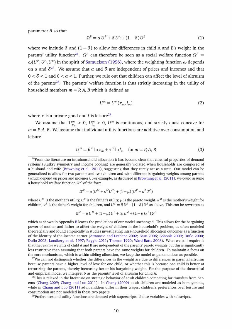
parameter δ so that

ΩP = αU P +δUA+ (1−δ)UB (1)

where we include δ and (1 − δ) to allow for differences in child A and B’s weight in the

parents’ utility function26. ΩP can therefore be seen as a social welfare function ΩP =ω(U P , UA, UB) in the spirit of Samuelson (1956), where the weighting function ω depends

on α and δ27. We assume that α and δ are independent of prices and incomes and that

0< δ < 1 and 0< α < 1. Further, we rule out that children can affect the level of altruism

of the parents28. The parents’ welfare function is thus strictly increasing in the utility of

household members m= P, A, B which is defined as

Um = Um(xm, lm) (2)

where x is a private good and l is leisure29.

We assume that Umxm> 0, Um

lm> 0, Um is continuous, and strictly quasi concave for

m= P, A, B. We assume that individual utility functions are additive over consumption and

leisure

Um = θm ln xm +τm ln lm for m= P, A, B (3)

26From the literature on intrahousehold allocation it has become clear that classical properties of demandsystems (Slutksy symmetry and income pooling) are generally violated when households are composed ofa husband and wife (Browning et al. 2011), suggesting that they rarely act as a unit. Our model can begeneralized to allow for two parents and two children and with different bargaining weights among parents(which depend on prices and incomes). For example, as discussed in Browning et al. (2011), we could assumea household welfare function Ω′P of the form

Ω′P = µ (U M + κM UC) + (1−µ) (U F +κF UC)

where U M is the mother’s utility, U F is the father’s utility, µ is the pareto weight, κM is the mother’s weight forchildren, κF is the father’s weight for children, and UC = δUA+(1−δ)UB as above. This can be rewritten as

Ω′P = µU M + (1−µ)U F + (µκM + (1−µ)κF )UC

which as shown in Appendix B leaves the predictions of our model unchanged. This allows for the bargainingpower of mother and father to affect the weight of children in the household’s problem, as often modeledtheoretically and found empirically in studies investigating intra-household allocation outcomes as a functionof the identity of the income earner (Attanasio and Lechene 2002; Basu 2006; Bobonis 2009; Duflo 2000;Duflo 2003; Lundberg et al. 1997; Reggio 2011; Thomas 1990; Ward-Batts 2008). What we still require isthat the relative weights of child A and B are independent of the parents’ pareto weights but this is significantlyless restrictive than assuming that both parents have the same weights for children. To maintain a focus onthe core mechanisms, which is within-sibling allocation, we keep the model as parsimonious as possible.

27We can not distinguish whether the differences in the weight are due to differences in parental altruismbecause parents have a higher level of love for one child, or whether this is because one child is better atterrorizing the parents, thereby increasing her or his bargaining weight. For the purpose of the theoreticaland empirical model we interpret δ as the parents’ level of altruism for child A.

28This is relaxed in the literature on strategic behavior of adult children competing for transfers from par-ents (Chang 2009; Chang and Luo 2011). In Chang (2009) adult children are modeled as homogenous,while in Chang and Luo (2011) adult children differ in their wages; children’s preferences over leisure andconsumption are not modeled in these two papers.

29Preferences and utility functions are denoted with superscripts, choice variables with subscripts.

10

so that θ measures household member m’s preferences for consumption and τ measures

his or her preferences for leisure; without loss of generality we set τP = 1. The use of a

log linear utility function for parents P and children A and B has two desirable properties.

First, it builds a concern for equity into the utilitarian welfare function ΩP , without ex-

plicitly modeling it through an additional parameter. Second, it allows us to obtain closed

form solutions which we can take directly to the data, establishing a clear link between the

theoretical model and the estimated parameters.

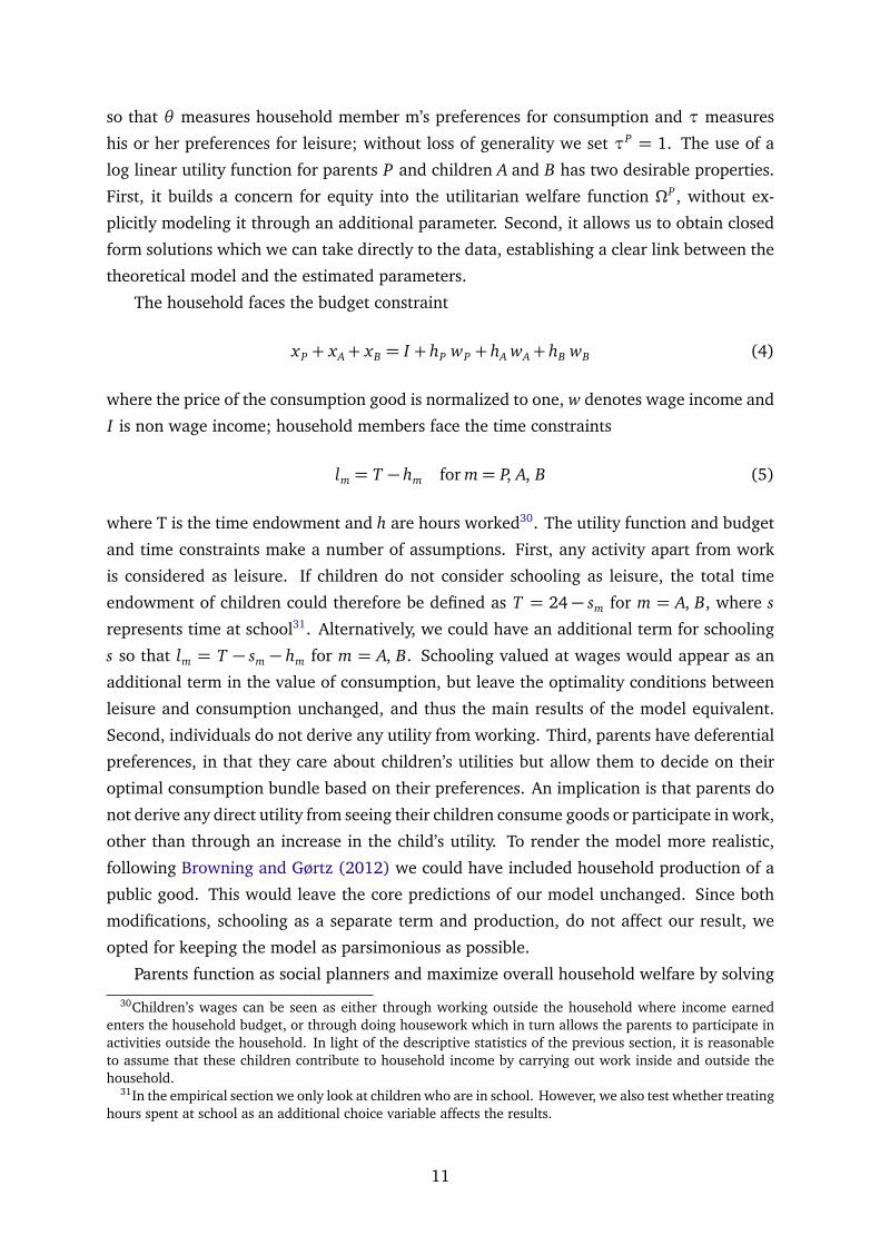
The household faces the budget constraint

xP + xA+ xB = I + hP wP + hA wA+ hB wB (4)

where the price of the consumption good is normalized to one, w denotes wage income and

I is non wage income; household members face the time constraints

lm = T − hm for m= P, A, B (5)

where T is the time endowment and h are hours worked30. The utility function and budget

and time constraints make a number of assumptions. First, any activity apart from work

is considered as leisure. If children do not consider schooling as leisure, the total time

endowment of children could therefore be defined as T = 24 − sm for m = A, B, where s

represents time at school31. Alternatively, we could have an additional term for schooling

s so that lm = T − sm − hm for m = A, B. Schooling valued at wages would appear as an

additional term in the value of consumption, but leave the optimality conditions between

leisure and consumption unchanged, and thus the main results of the model equivalent.

Second, individuals do not derive any utility from working. Third, parents have deferential

preferences, in that they care about children’s utilities but allow them to decide on their

optimal consumption bundle based on their preferences. An implication is that parents do

not derive any direct utility from seeing their children consume goods or participate in work,

other than through an increase in the child’s utility. To render the model more realistic,

following Browning and Gørtz (2012) we could have included household production of a

public good. This would leave the core predictions of our model unchanged. Since both

modifications, schooling as a separate term and production, do not affect our result, we

opted for keeping the model as parsimonious as possible.

Parents function as social planners and maximize overall household welfare by solving

30Children’s wages can be seen as either through working outside the household where income earnedenters the household budget, or through doing housework which in turn allows the parents to participate inactivities outside the household. In light of the descriptive statistics of the previous section, it is reasonableto assume that these children contribute to household income by carrying out work inside and outside thehousehold.

31In the empirical section we only look at children who are in school. However, we also test whether treatinghours spent at school as an additional choice variable affects the results.

11

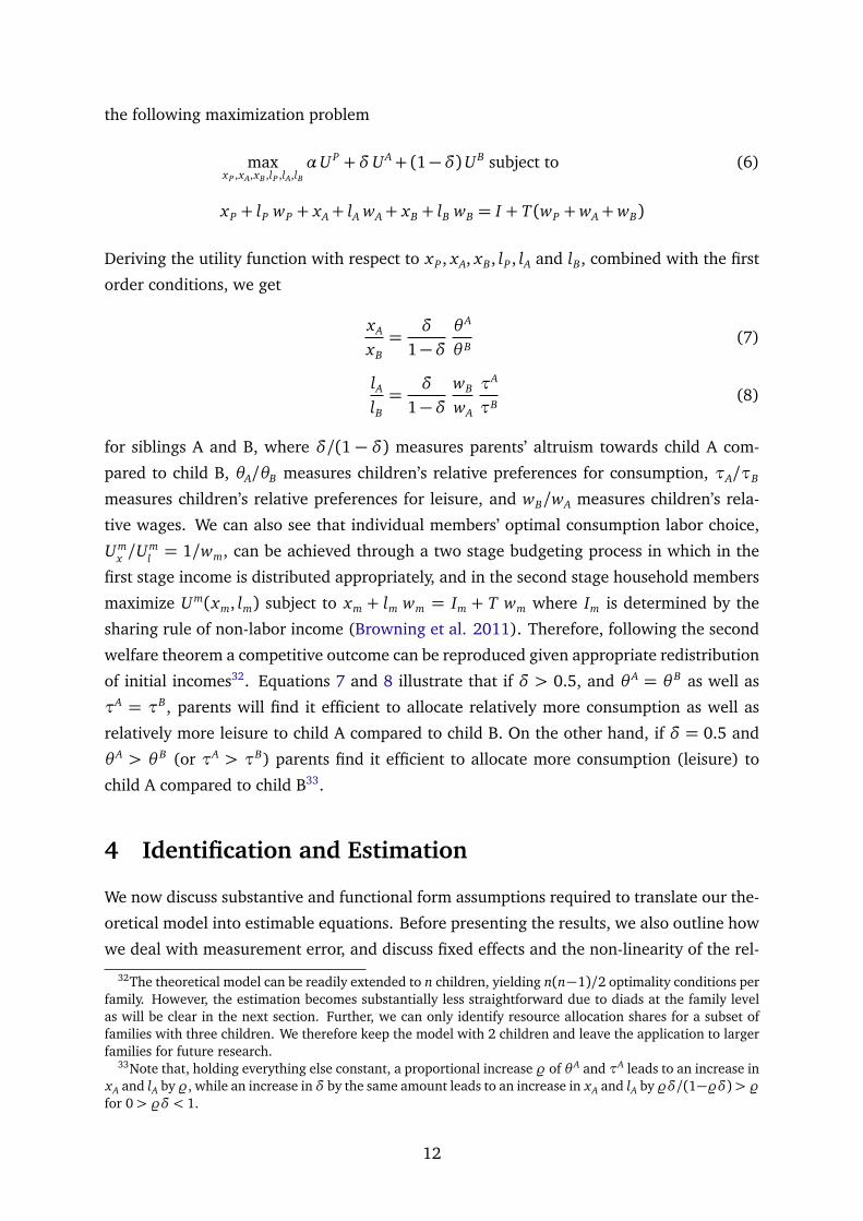
the following maximization problem

maxxP ,xA,xB ,lP ,lA,lB

αU P +δUA+ (1−δ)UB subject to (6)

xP + lP wP + xA+ lA wA+ xB + lB wB = I + T (wP +wA+wB)

Deriving the utility function with respect to xP , xA, xB, lP , lA and lB, combined with the first

order conditions, we get

xA

xB=

δ

1−δθA

θ B(7)

lAlB=

δ

1−δwB

wA

τA

τB(8)

for siblings A and B, where δ/(1 − δ) measures parents’ altruism towards child A com-

pared to child B, θA/θB measures children’s relative preferences for consumption, τA/τB

measures children’s relative preferences for leisure, and wB/wA measures children’s rela-

tive wages. We can also see that individual members’ optimal consumption labor choice,

Umx /U

ml = 1/wm, can be achieved through a two stage budgeting process in which in the

first stage income is distributed appropriately, and in the second stage household members

maximize Um(xm, lm) subject to xm + lm wm = Im + T wm where Im is determined by the

sharing rule of non-labor income (Browning et al. 2011). Therefore, following the second

welfare theorem a competitive outcome can be reproduced given appropriate redistribution

of initial incomes32. Equations 7 and 8 illustrate that if δ > 0.5, and θA = θ B as well as

τA = τB, parents will find it efficient to allocate relatively more consumption as well as

relatively more leisure to child A compared to child B. On the other hand, if δ = 0.5 and

θA > θ B (or τA > τB) parents find it efficient to allocate more consumption (leisure) to

child A compared to child B33.

4 Identification and Estimation

We now discuss substantive and functional form assumptions required to translate our the-

oretical model into estimable equations. Before presenting the results, we also outline how

we deal with measurement error, and discuss fixed effects and the non-linearity of the rel-

32The theoretical model can be readily extended to n children, yielding n(n−1)/2 optimality conditions perfamily. However, the estimation becomes substantially less straightforward due to diads at the family levelas will be clear in the next section. Further, we can only identify resource allocation shares for a subset offamilies with three children. We therefore keep the model with 2 children and leave the application to largerfamilies for future research.

33Note that, holding everything else constant, a proportional increase % of θA and τA leads to an increase inxA and lA by%, while an increase in δ by the same amount leads to an increase in xA and lA by%δ/(1−%δ)> %for 0> %δ < 1.

12

ative expenditures variable.

4.1 Substantive Assumptions

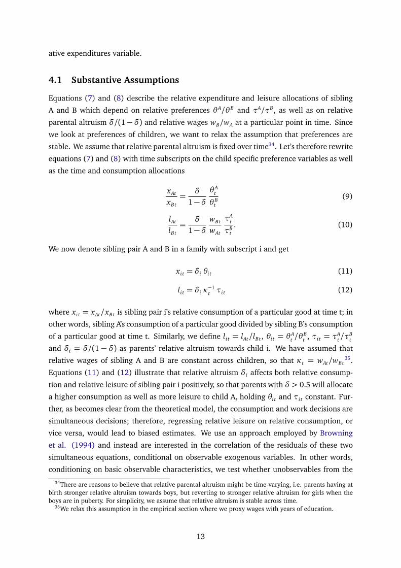
Equations (7) and (8) describe the relative expenditure and leisure allocations of sibling

A and B which depend on relative preferences θA/θ B and τA/τB, as well as on relative

parental altruism δ/(1− δ) and relative wages wB/wA at a particular point in time. Since

we look at preferences of children, we want to relax the assumption that preferences are

stable. We assume that relative parental altruism is fixed over time34. Let’s therefore rewrite

equations (7) and (8) with time subscripts on the child specific preference variables as well

as the time and consumption allocations

xAt

xBt=

δ

1−δθA

t

θ Bt

(9)

lAt

lBt=

δ

1−δwBt

wAt

τAt

τBt. (10)

We now denote sibling pair A and B in a family with subscript i and get

x i t = δi θi t (11)

li t = δi κ−1t τi t (12)

where x i t = xAt/xBt is sibling pair i’s relative consumption of a particular good at time t; in

other words, sibling A’s consumption of a particular good divided by sibling B’s consumption

of a particular good at time t. Similarly, we define li t = lAt/lBt , θi t = θAt /θ

Bt , τi t = τA

t /τBt

and δi = δ/(1 − δ) as parents’ relative altruism towards child i. We have assumed that

relative wages of sibling A and B are constant across children, so that κt = wAt/wBt35.

Equations (11) and (12) illustrate that relative altruism δi affects both relative consump-

tion and relative leisure of sibling pair i positively, so that parents with δ > 0.5 will allocate

a higher consumption as well as more leisure to child A, holding θi t and τi t constant. Fur-

ther, as becomes clear from the theoretical model, the consumption and work decisions are

simultaneous decisions; therefore, regressing relative leisure on relative consumption, or

vice versa, would lead to biased estimates. We use an approach employed by Browning

et al. (1994) and instead are interested in the correlation of the residuals of these two

simultaneous equations, conditional on observable exogenous variables. In other words,

conditioning on basic observable characteristics, we test whether unobservables from the

34There are reasons to believe that relative parental altruism might be time-varying, i.e. parents having atbirth stronger relative altruism towards boys, but reverting to stronger relative altruism for girls when theboys are in puberty. For simplicity, we assume that relative altruism is stable across time.

35We relax this assumption in the empirical section where we proxy wages with years of education.

13

time allocation decision are correlated with unobservables from the consumption decision.

4.2 Functional Form Assumptions

We model children’s relative preferences for consumption and leisure at time t as a func-

tion of a vector of observable household and child characteristics Z i t which include age,

gender, rural or urban location, and a time fixed effect; further, we assume the presence

of unobservable time invariant individual fixed effects λθ i and λτi, as well as time-varying

idiosyncratic error terms εθ i t and ετi t unobserved by the econometrician, yielding

θi t = expβθ0+ β ′

θZ i t +λθ i + εθ i t (13)

τi t = expβτ0+ β ′

τZ i t +λτi + ετi t. (14)

Birth order or relative birth order have proven to be important determinants of within

household allocation (Black et al. 2005; Chesnokova and Vaithianathan 2008; Ejrnæs and

Pörtner 2004; Patrinos and Psacharopoulos 1997). It would therefore be a natural candi-

date to model relative altruism. However, it is highly correlated with the age difference.

Second, it does not satisfy the exclusion restriction that the effect of birth order Ri t is equal

to zero in a regression of the difference between relative expenditure and relative leisure

on birth order3637. We therefore assume that parents’ relative altruism for child A versus

child B is a function of an unobservable time invariant individual fixed effect λδi

δi = expβδ0+λδi. (15)

4.3 Measurement Error

Until now we assumed that we know the true level of expenditures and leisure. However,

in addition to recall bias, due to the nature of the data there is a second source of likely

measurement error, illustrated in detail in the appendix in section C. We know the allocation

to the panel child as a fraction of the expenditure category (boys or girls clothes). We

therefore always denote the panel child as child A. However, expenditures allocated to the

sibling of the panel child are vulnerable to measurement error, since we assume that parents

list clothes for household members 18 and over in the adult clothes category. Therefore,

36The exclusion restriction emerges from taking the ratio of equations (11) and (12), and taking logs. Thisremoves δi so that we require βδ1 = 0 in

ln x i t − ln li t = βδ0 + βδ1 Ri +β′δ2 Z i t + εδi t .

In other words, conditional on Z i t , a variable Ri proxying for altruism should not affect ln x i t − ln li t .37We have also tested including a dummy variable which is equal to one if the oldest sibling is a boy

(unconditional on whether he has a younger brother or a sister) and if the oldest sibling is a boy with a sister,but the variables do not pass the exclusion restriction or only marginally pass it, so we do not include them.

14

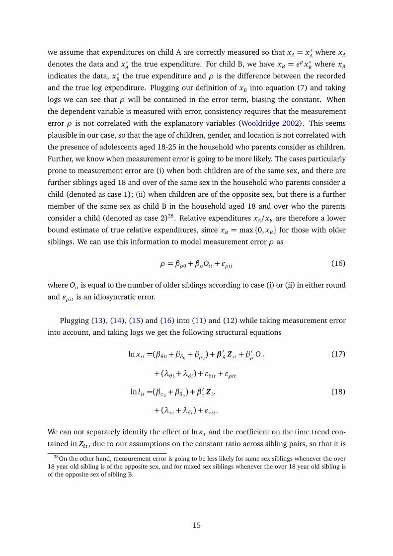
we assume that expenditures on child A are correctly measured so that xA = x∗A where xA

denotes the data and x∗A the true expenditure. For child B, we have xB = eρ x∗B where xB

indicates the data, x∗B the true expenditure and ρ is the difference between the recorded

and the true log expenditure. Plugging our definition of xB into equation (7) and taking

logs we can see that ρ will be contained in the error term, biasing the constant. When

the dependent variable is measured with error, consistency requires that the measurement

error ρ is not correlated with the explanatory variables (Wooldridge 2002). This seems

plausible in our case, so that the age of children, gender, and location is not correlated with

the presence of adolescents aged 18-25 in the household who parents consider as children.

Further, we know when measurement error is going to be more likely. The cases particularly

prone to measurement error are (i) when both children are of the same sex, and there are

further siblings aged 18 and over of the same sex in the household who parents consider a

child (denoted as case 1); (ii) when children are of the opposite sex, but there is a further

member of the same sex as child B in the household aged 18 and over who the parents

consider a child (denoted as case 2)38. Relative expenditures xA/xB are therefore a lower

bound estimate of true relative expenditures, since xB = max 0, xB for those with older

siblings. We can use this information to model measurement error ρ as

ρ = βρ0 + βρOi t + ερi t (16)

where Oi t is equal to the number of older siblings according to case (i) or (ii) in either round

and ερi t is an idiosyncratic error.

Plugging (13), (14), (15) and (16) into (11) and (12) while taking measurement error

into account, and taking logs we get the following structural equations

ln x i t =(βθ0 + βδ0+ βρ0

) +β ′θ

Z i t + β′ρ

Oi t (17)

+ (λθ i +λδi) + εθ i t + ερi t

ln li t =(βτ0+ βδ0

) + β ′τ

Z i t (18)

+ (λτi +λδi) + ετi t .

We can not separately identify the effect of lnκt and the coefficient on the time trend con-

tained in Zi t , due to our assumptions on the constant ratio across sibling pairs, so that it is

38On the other hand, measurement error is going to be less likely for same sex siblings whenever the over18 year old sibling is of the opposite sex, and for mixed sex siblings whenever the over 18 year old sibling isof the opposite sex of sibling B.

15

part of Zi t . We then get the two linear reduced forms

ln x i t =Πx0 +Π′xθ Z i t +Π

′xρ Oi t + εx i t (19)

ln li t =Πl0 +Π′lτ Z i t + εl i t . (20)

Identification of Πxθ , Πlτ, and Πxρ requires that Z i t , and Oi t are uncorrelated with the

composite error terms εx i t and εl i t . This is not an implausible assumption given that age,

gender and location are out of the control of the child. We test the two following proposi-

tions adopted from Browning and Gørtz (2012):

Proposition 1 (Differences in children’s preferences) If θi t and τi t are negatively correlated,

there is no variation in δi and wBt = wAt , then x i t and li t will be negatively correlated.

Proposition 2 (Differences in parental altruism) If there is variation in δi while θi t and τi t

are independent of each other and wBt = wAt , x i t and li t will be positively correlated.

The empirical model shows that if differences in parental altruism drive allocations and

preferences for leisure and consumption are independent, we expect the residuals to be

positively correlated due to the fact that they both contain λδi and altruism affects con-

sumption and leisure positively. If heterogeneity is due to differences in children’s tastes, so

that if relative preferences for leisure and consumption are negatively correlated and the

there is no variation in relative altruism, then we expect the residuals to be negatively cor-

related as they contain (λθ i+εθ i) and (λτi+ετi). Propositions 1 and 2 present the extreme

cases. It is reasonable to assume, and we can not rule out, that both relative altruism and

relative preferences play a role in determining outcomes. For example, if we find a strong

negative correlation of the residuals in the empirical application this does not imply that

parents do not have different weights for their children. It only indicates that results are

consistent with a model in which differences in preferences are the dominant driver of al-

locations rather than differences in parental altruism. The empirical section also presents

a battery of robustness tests to distinguish between alternative explanations that might be

driving the results.

4.4 Estimation: Fixed Effects and Non-Linearity of the Expenditure

Variable

Despite having a panel, a consistent estimation of the fixed effects (λθ i+λδi) and (λτi+λδi)is not feasible. First, with two time periods, it is not possible to obtain a consistent estimate

of the fixed effect (Wooldridge 2002). Second, several of the preference parameters are

time invariant; even for more time periods we would only be able to identify a combination

of the fixed effect and the coefficient on the time invariant variables. Instead of using the

16

natural logarithm, we follow Browning et al. (1994) and transform x i t and li t using the

inverse hyperbolic sine39. Inspection of the distribution of x i t and li t in figures 2 to 5 also

showed that these variables are clumped at specific values, which is particularly true for

x i t . The nature of the questionnaire is the reason for this clumping at various points. As

discussed in the previous section, parents were asked to indicate the approximate fraction

of expenditures that went to the index child, measured by a variable ranging from 1 to 5. In

order to take into account the non-continuous nature of the variable, we also model relative

expenditures and relative leisure as ordered variables, taking on three values

v∗i t =

0 if vi t < 1

1 if vi t = 1

2 if vi t > 1

(21)

for v = l, x . We present estimates for treating both variables as continuous, x i t as an or-

dered variable and li t as continuous, and both variables as ordered. For all models, we

jointly estimate equations (19) and (20) with full information maximum likelihood, as-

suming that the errors have a bivariate normal distribution, and then test the correlation

of the error terms of the two equations. The estimation is performed using the command

cmp as developed by Roodman (2009).

5 Empirical Results and Discussion

5.1 Base Results

We start by looking at the unconditional distribution of leisure and consumption. Figure

1 shows the joint distribution of relative expenditure and leisure overlaid with a linear

and a local polynomial regression and a 95 percent confidence interval. The figures show

that there is a significant, negative, and fairly linear relationship between siblings’ relative

consumption and leisure for India, Peru and Vietnam. For the empirical model, we present

results for the different specifications of the dependent variables. Column (1) presents

the results for both variables modeled as continuous, column (2) models x i t as ordered

and li t as continuous, and column (3) models both variables as ordered. We present the

correlations of the residuals as this allows us later to purge relative leisure and relative

consumption from the effects of age and gender. The correlation of the residuals is shown

following the estimated coefficients.

39The main advantage of this transformation is that the inverse hyperbolic sine is always positive and linearfor low values, but very similar to the natural logarithm for high values. This avoids having highly negativevalues when relative expenditure and relative leisure are very low. Even though it is defined for the whole realline, so including zero, we do not include relative expenditure or leisure that is equal to zero. Our results aresubstantively unchanged when using the natural logarithm instead of the inverse hyperbolic sine; the choicebetween the inverse hyperbolic sine and the natural logarithm is therefore not fundamental for the results.

17

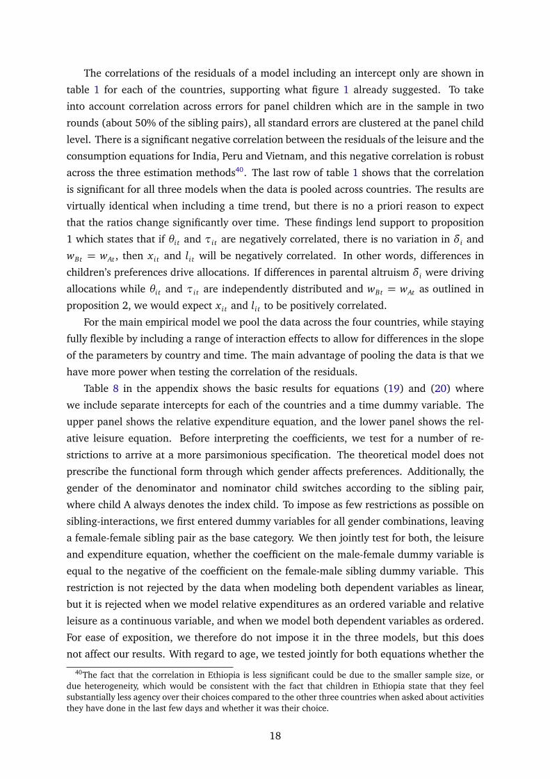
The correlations of the residuals of a model including an intercept only are shown in

table 1 for each of the countries, supporting what figure 1 already suggested. To take

into account correlation across errors for panel children which are in the sample in two

rounds (about 50% of the sibling pairs), all standard errors are clustered at the panel child

level. There is a significant negative correlation between the residuals of the leisure and the

consumption equations for India, Peru and Vietnam, and this negative correlation is robust

across the three estimation methods40. The last row of table 1 shows that the correlation

is significant for all three models when the data is pooled across countries. The results are

virtually identical when including a time trend, but there is no a priori reason to expect

that the ratios change significantly over time. These findings lend support to proposition

1 which states that if θi t and τi t are negatively correlated, there is no variation in δi and

wBt = wAt , then x i t and li t will be negatively correlated. In other words, differences in

children’s preferences drive allocations. If differences in parental altruism δi were driving

allocations while θi t and τi t are independently distributed and wBt = wAt as outlined in

proposition 2, we would expect x i t and li t to be positively correlated.

For the main empirical model we pool the data across the four countries, while staying

fully flexible by including a range of interaction effects to allow for differences in the slope

of the parameters by country and time. The main advantage of pooling the data is that we

have more power when testing the correlation of the residuals.

Table 8 in the appendix shows the basic results for equations (19) and (20) where

we include separate intercepts for each of the countries and a time dummy variable. The

upper panel shows the relative expenditure equation, and the lower panel shows the rel-

ative leisure equation. Before interpreting the coefficients, we test for a number of re-

strictions to arrive at a more parsimonious specification. The theoretical model does not

prescribe the functional form through which gender affects preferences. Additionally, the

gender of the denominator and nominator child switches according to the sibling pair,

where child A always denotes the index child. To impose as few restrictions as possible on

sibling-interactions, we first entered dummy variables for all gender combinations, leaving

a female-female sibling pair as the base category. We then jointly test for both, the leisure

and expenditure equation, whether the coefficient on the male-female dummy variable is

equal to the negative of the coefficient on the female-male sibling dummy variable. This

restriction is not rejected by the data when modeling both dependent variables as linear,

but it is rejected when we model relative expenditures as an ordered variable and relative

leisure as a continuous variable, and when we model both dependent variables as ordered.

For ease of exposition, we therefore do not impose it in the three models, but this does

not affect our results. With regard to age, we tested jointly for both equations whether the

40The fact that the correlation in Ethiopia is less significant could be due to the smaller sample size, ordue heterogeneity, which would be consistent with the fact that children in Ethiopia state that they feelsubstantially less agency over their choices compared to the other three countries when asked about activitiesthey have done in the last few days and whether it was their choice.

18

coefficient on the age of child A is equal to the negative of the coefficient on the age of child

B which is not rejected in any of the models. We can therefore impose the restriction that

age affects relative expenditure and leisure through the difference in age of child A and B41.

We now discuss the parsimonious specification presented in table 2. The results show

that the coefficients on relative age are statistically significantly different from zero in both

the leisure and the expenditure equation, and this holds for any specification of the de-

pendent variables. We find that the larger the age difference between child A and B, the

higher is relative expenditure and the lower is relative leisure. For mixed sibling pairs, an

interesting pattern arises. When the index child is female and has a brother, she enjoys

significantly higher expenditure and significantly lower leisure compared to a female index

child with a sister. The effect is significant also for male index children who have a sister,

who enjoy significantly higher leisure compared to female index children with a sister. The

control for whether the child lives in an urban area is insignificant which suggests that there

are no systematic differences across urban and rural settings that would lead to more or

less equal relative expenditure or relative leisure patterns. The coefficient on the variable

capturing measurement error is negative, in line with our conjecture, indicating that our

measure of relative expenditure is systematically lower when one of the two outlined cases

of measurement error takes place.

The negative correlation in the relative leisure-consumption relationship we observed in

the unconditional distribution graphs could have been driven simply by the fact that older

children have less leisure if they get a younger sibling due to longer hours of caretaking, but

they get higher expenditures since they are the oldest and parents need to build up a stock of

children’s clothes and other child-related items. In the same logic, younger children could

get more leisure (playing time) as they are younger and less clothes expenditures due to the

fact that their older sibling passes them on clothes. However, this does not appear to be the

case as even after controlling for the age difference and gender composition, the negative

correlation of the residuals persists. The last row in table 2 shows that the correlation of

the residuals is substantially lower with a correlation of about -0.05 compared to -0.2 in

table 1 but it remains negative, and is statistically significantly different from zero when

estimating the model as a an ordered probit with a linear model in column (2), or as two

ordered probit equations in column (3). The correlation in the residuals is negative as

well in column (1) when both variables are modeled as continuous variables, although

statistically not significantly different from zero. Given the discontinuous distribution of in

particular the expenditure variable, it is not surprising that the model performs better when

taking the structure of the data into account. Thus, our preferred specification is column

(2). The results, modeling both variables as ordered variables, are very similar.

41When testing these restrictions with a set of likelihood ratio tests, we are not able to cluster standarderrors at the child level. We have also estimated the models without imposing any restrictions and the resultsremain robust.

19

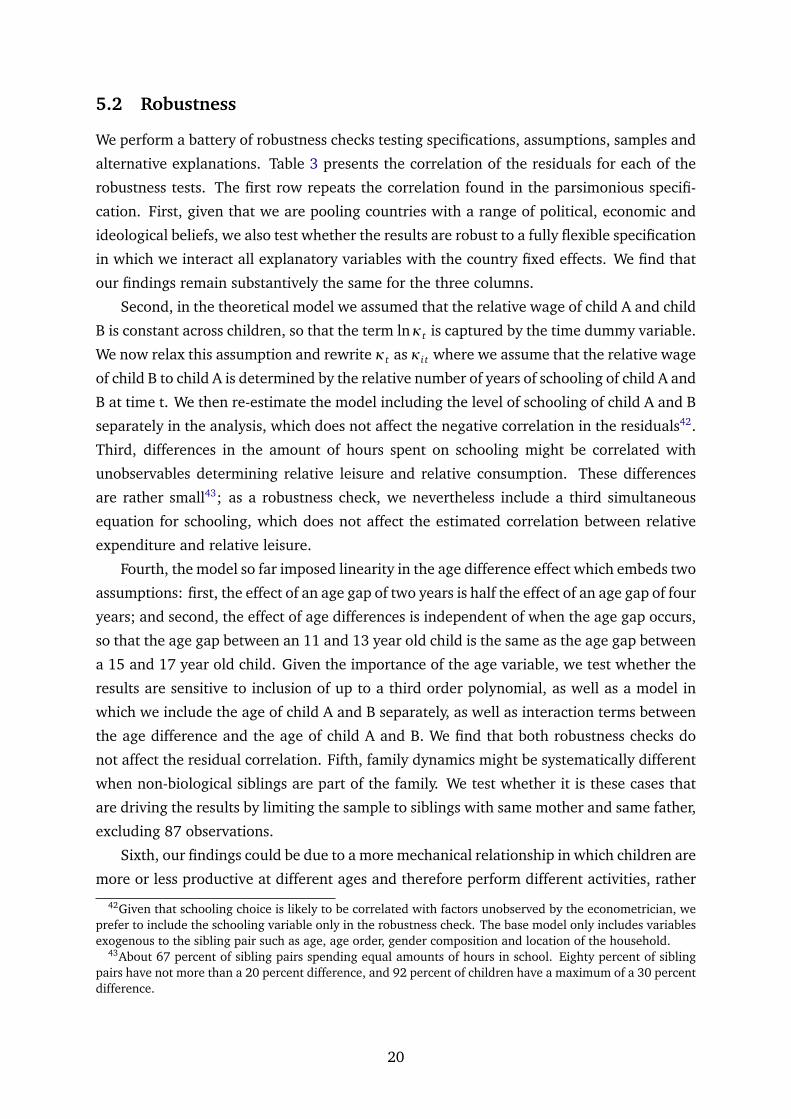
5.2 Robustness

We perform a battery of robustness checks testing specifications, assumptions, samples and

alternative explanations. Table 3 presents the correlation of the residuals for each of the

robustness tests. The first row repeats the correlation found in the parsimonious specifi-

cation. First, given that we are pooling countries with a range of political, economic and

ideological beliefs, we also test whether the results are robust to a fully flexible specification

in which we interact all explanatory variables with the country fixed effects. We find that

our findings remain substantively the same for the three columns.

Second, in the theoretical model we assumed that the relative wage of child A and child

B is constant across children, so that the term lnκt is captured by the time dummy variable.

We now relax this assumption and rewrite κt as κi t where we assume that the relative wage

of child B to child A is determined by the relative number of years of schooling of child A and

B at time t. We then re-estimate the model including the level of schooling of child A and B

separately in the analysis, which does not affect the negative correlation in the residuals42.

Third, differences in the amount of hours spent on schooling might be correlated with

unobservables determining relative leisure and relative consumption. These differences

are rather small43; as a robustness check, we nevertheless include a third simultaneous

equation for schooling, which does not affect the estimated correlation between relative

expenditure and relative leisure.

Fourth, the model so far imposed linearity in the age difference effect which embeds two

assumptions: first, the effect of an age gap of two years is half the effect of an age gap of four

years; and second, the effect of age differences is independent of when the age gap occurs,

so that the age gap between an 11 and 13 year old child is the same as the age gap between

a 15 and 17 year old child. Given the importance of the age variable, we test whether the

results are sensitive to inclusion of up to a third order polynomial, as well as a model in

which we include the age of child A and B separately, as well as interaction terms between

the age difference and the age of child A and B. We find that both robustness checks do

not affect the residual correlation. Fifth, family dynamics might be systematically different

when non-biological siblings are part of the family. We test whether it is these cases that

are driving the results by limiting the sample to siblings with same mother and same father,

excluding 87 observations.

Sixth, our findings could be due to a more mechanical relationship in which children are

more or less productive at different ages and therefore perform different activities, rather

42Given that schooling choice is likely to be correlated with factors unobserved by the econometrician, weprefer to include the schooling variable only in the robustness check. The base model only includes variablesexogenous to the sibling pair such as age, age order, gender composition and location of the household.

43About 67 percent of sibling pairs spending equal amounts of hours in school. Eighty percent of siblingpairs have not more than a 20 percent difference, and 92 percent of children have a maximum of a 30 percentdifference.

20

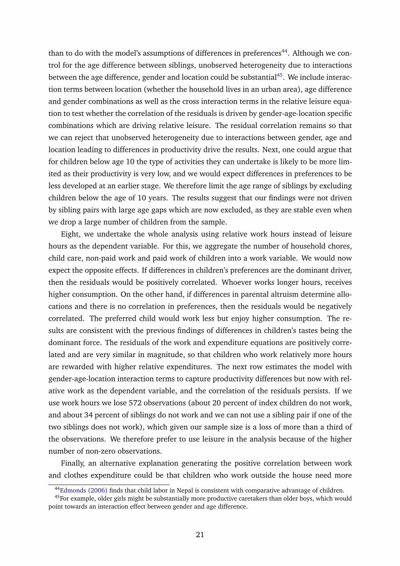
than to do with the model’s assumptions of differences in preferences44. Although we con-

trol for the age difference between siblings, unobserved heterogeneity due to interactions

between the age difference, gender and location could be substantial45. We include interac-

tion terms between location (whether the household lives in an urban area), age difference

and gender combinations as well as the cross interaction terms in the relative leisure equa-

tion to test whether the correlation of the residuals is driven by gender-age-location specific

combinations which are driving relative leisure. The residual correlation remains so that

we can reject that unobserved heterogeneity due to interactions between gender, age and

location leading to differences in productivity drive the results. Next, one could argue that

for children below age 10 the type of activities they can undertake is likely to be more lim-

ited as their productivity is very low, and we would expect differences in preferences to be

less developed at an earlier stage. We therefore limit the age range of siblings by excluding

children below the age of 10 years. The results suggest that our findings were not driven

by sibling pairs with large age gaps which are now excluded, as they are stable even when

we drop a large number of children from the sample.

Eight, we undertake the whole analysis using relative work hours instead of leisure

hours as the dependent variable. For this, we aggregate the number of household chores,

child care, non-paid work and paid work of children into a work variable. We would now

expect the opposite effects. If differences in children’s preferences are the dominant driver,

then the residuals would be positively correlated. Whoever works longer hours, receives

higher consumption. On the other hand, if differences in parental altruism determine allo-

cations and there is no correlation in preferences, then the residuals would be negatively

correlated. The preferred child would work less but enjoy higher consumption. The re-

sults are consistent with the previous findings of differences in children’s tastes being the

dominant force. The residuals of the work and expenditure equations are positively corre-

lated and are very similar in magnitude, so that children who work relatively more hours

are rewarded with higher relative expenditures. The next row estimates the model with

gender-age-location interaction terms to capture productivity differences but now with rel-

ative work as the dependent variable, and the correlation of the residuals persists. If we

use work hours we lose 572 observations (about 20 percent of index children do not work,

and about 34 percent of siblings do not work and we can not use a sibling pair if one of the

two siblings does not work), which given our sample size is a loss of more than a third of

the observations. We therefore prefer to use leisure in the analysis because of the higher

number of non-zero observations.

Finally, an alternative explanation generating the positive correlation between work

and clothes expenditure could be that children who work outside the house need more

44Edmonds (2006) finds that child labor in Nepal is consistent with comparative advantage of children.45For example, older girls might be substantially more productive caretakers than older boys, which would

point towards an interaction effect between gender and age difference.

21

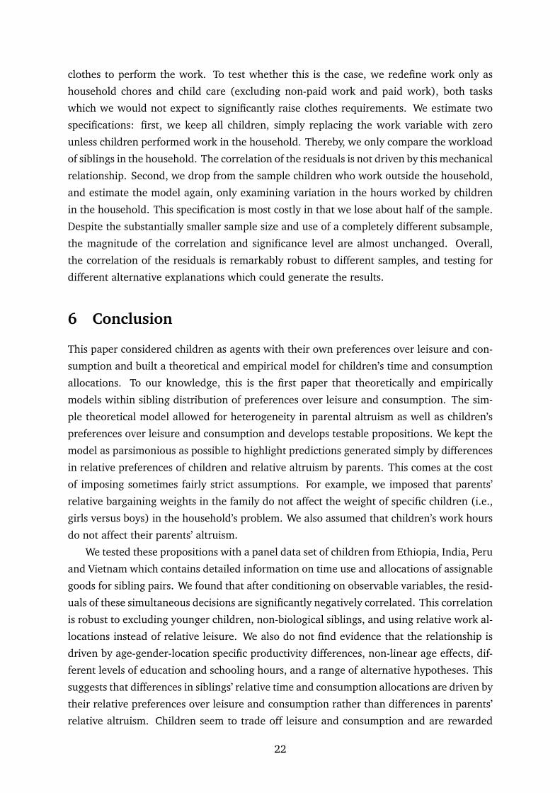
clothes to perform the work. To test whether this is the case, we redefine work only as

household chores and child care (excluding non-paid work and paid work), both tasks

which we would not expect to significantly raise clothes requirements. We estimate two

specifications: first, we keep all children, simply replacing the work variable with zero

unless children performed work in the household. Thereby, we only compare the workload

of siblings in the household. The correlation of the residuals is not driven by this mechanical

relationship. Second, we drop from the sample children who work outside the household,

and estimate the model again, only examining variation in the hours worked by children

in the household. This specification is most costly in that we lose about half of the sample.

Despite the substantially smaller sample size and use of a completely different subsample,

the magnitude of the correlation and significance level are almost unchanged. Overall,

the correlation of the residuals is remarkably robust to different samples, and testing for

different alternative explanations which could generate the results.

6 Conclusion

This paper considered children as agents with their own preferences over leisure and con-

sumption and built a theoretical and empirical model for children’s time and consumption

allocations. To our knowledge, this is the first paper that theoretically and empirically

models within sibling distribution of preferences over leisure and consumption. The sim-

ple theoretical model allowed for heterogeneity in parental altruism as well as children’s

preferences over leisure and consumption and develops testable propositions. We kept the

model as parsimonious as possible to highlight predictions generated simply by differences

in relative preferences of children and relative altruism by parents. This comes at the cost

of imposing sometimes fairly strict assumptions. For example, we imposed that parents’

relative bargaining weights in the family do not affect the weight of specific children (i.e.,

girls versus boys) in the household’s problem. We also assumed that children’s work hours

do not affect their parents’ altruism.

We tested these propositions with a panel data set of children from Ethiopia, India, Peru

and Vietnam which contains detailed information on time use and allocations of assignable

goods for sibling pairs. We found that after conditioning on observable variables, the resid-

uals of these simultaneous decisions are significantly negatively correlated. This correlation

is robust to excluding younger children, non-biological siblings, and using relative work al-

locations instead of relative leisure. We also do not find evidence that the relationship is

driven by age-gender-location specific productivity differences, non-linear age effects, dif-

ferent levels of education and schooling hours, and a range of alternative hypotheses. This

suggests that differences in siblings’ relative time and consumption allocations are driven by

their relative preferences over leisure and consumption rather than differences in parents’

relative altruism. Children seem to trade off leisure and consumption and are rewarded

22

accordingly. As a result, the data are consistent with a model in which families behave as

if they were an internal market in which children select their optimal consumption-leisure

bundle.

One implication of this finding is that in order to understand households’ behavior in low

income countries, it is important to consider heterogeneity in children’s preferences. Given

the stringent data requirements, we were able to undertake this analysis for families with

two children between the ages of 6-17 years in four developing countries. To investigate

the generalizability of the results, future research should focus on extending the analysis to

families with more than two children and application to further countries.

23

References

Andersen, S., S. Ertac, U. Gneezy, J. A. List, and S. Maximiano (2013). Gender, com-

petitiveness and socialization at a young age: evidence from a matrilineal and a

patriarchal society. Review of Economics and Statistics 95(4), 1438–1443.

Attanasio, O., E. Fitzsimons, A. Gomez, M. I. Gutierrez, C. Meghir, and A. Mesnard

(2010). Children’s schooling and work in the presence of a conditional cash transfer

program in rural colombia. Economic development and cultural change 58(2), 181–

210.

Attanasio, O. and V. Lechene (2002). Tests of income pooling in household decisions.

Review of economic dynamics 5(4), 720–748.

Barcellos, S. H., L. S. Carvalho, and A. Lleras-Muney (2014). Child gender and parental

investments in india: Are boys and girls treated differently? American Economic

Journal: Applied Economics 6(1), 157–89.

Basu, K. (2006). Gender and say: a model of household behaviour with endogenously

determined balance of power. The Economic Journal 116(511), 558–580.

Becker, G. (1981). A Treatise on the Family. Harvard Univ Press.

Becker, G. S. and H. G. Lewis (1973). On the interaction between the quantity and quality

of children. Journal of Political Economy 81(2), S279–88.

Becker, G. S. and N. Tomes (1976). Child endowments and the quantity and quality of

children. The Journal of Political Economy 84(4), S143–S162.

Behrman, J. R. (1997). Intrahousehold distribution and the family. Handbook of Popula-

tion and Family Economics 1, 125–187.

Behrman, J. R., R. A. Pollak, and P. Taubman (1982). Parental preferences and provision

for progeny. The Journal of Political Economy, 52–73.

Behrman, J. R., R. A. Pollak, and P. Taubman (1995). From parent to child: Intrahousehold

allocations and intergenerational relations in the United States. University of Chicago

Press.

Behrman, J. R., M. R. Rosenzweig, and P. Taubman (1994). Endowments and the allo-

cation of schooling in the family and in the marriage market: the twins experiment.

Journal of Political Economy, 1131–1174.

Berry, J. (2013). Child control in education decisions: an evaluation of targeted incen-

tives to learn in India. Unpublished manuscript.

Black, S. E., P. J. Devereux, and K. G. Salvanes (2005). The more the merrier? the

effect of family size and birth order on children’s education. The Quarterly Journal of

Economics 120(2), 669–700.

24

Blundell, R., P.-A. Chiappori, and C. Meghir (2005, December). Collective labor supply

with children. Journal of Political Economy 113(6), 1277–1306.

Bobonis, G. (2009). Is the allocation of resources within the household efficient? new

evidence from a randomized experiment. Journal of Political Economy 117(3), 453–

503.

Bonke, J. and M. Browning (2011). Spending on children: Direct survey evidence. The

Economic Journal 121(554), F123–F143.

Browning, M. (1992). Children and household economic behavior. Journal of Economic

Literature, 1434–1475.

Browning, M., F. Bourguignon, P. Chiappori, and V. Lechene (1994). Income and out-

comes: a structural model of intrahousehold allocation. Journal of Political Econ-

omy 102(6), 1067–1096.

Browning, M. and P. Chiappori (1998). Efficient intra-household allocations: A general

characterization and empirical tests. Econometrica 66(6), 1241–1278.

Browning, M., P. Chiappori, and Y. Weiss (2011). Family Economics. Unpublished Text-

book Manuscript, Tel Aviv University.

Browning, M. and M. Ejrnæs (2009). Consumption and children. The Review of Economics

and Statistics 91(1), 93–111.

Browning, M. and M. Gørtz (2012). Spending time and money within the household.

The Scandinavian Journal of Economics 114(3), 681–704.

Browning, M. and V. Lechene (2003). Children and demand: direct and non-direct ef-

fects. Review of Economics of the Household 1(1), 9–31.

Bursztyn, L. and L. C. Coffman (2012). The schooling decision: Family preferences, in-

tergenerational conflict, and moral hazard in the brazilian favelas. Journal of Political

Economy 120(3), 359–397.

Castillo, M., P. J. Ferraro, J. L. Jordan, and R. Petrie (2011). The today and tomorrow

of kids: Time preferences and educational outcomes of children. Journal of Public

Economics 95(11), 1377–1385.

Chang, Y. (2009). Strategic altruistic transfers and rent seeking within the family. Journal

of Population Economics 22(4), 1081–1098.

Chang, Y.-M. and Z. Luo (2011). Endogenous division rules as a family constitution:

Strategic altruistic transfers and sibling competition. Technical report.

Cherchye, L., B. De Rock, and F. Vermeulen (2012). Married with children: A collective

labor supply model with detailed time use and intrahousehold expenditure informa-

tion. American Economic Review 102(7), 3377–3405.

25

Chesnokova, T. and R. Vaithianathan (2008). Lucky last? intra-sibling allocation of child

labor. The BE Journal of Economic Analysis & Policy 8(1).

Chiappori, P. (1988). Rational household labor supply. Econometrica: Journal of the

Econometric Society, 63–90.

Conti, G., J. J. Heckman, J. Yi, and J. Zhang (2010). Early health shocks, parental re-

sponses, and child outcomes. Unpublished manuscript.

Crook, M. (1937). Intra-family relationships in personality test performance. The Psy-

chological Record 1, 479–502.

Daniels, D. and R. Plomin (1985). Differential experience of siblings in the same family.

Developmental Psychology 21(5), 747.

Dauphin, A., A. El Lahga, B. Fortin, and G. Lacroix (2010). Are children decision-makers

within the household? The Economic Journal.

Dornbusch, S., J. Carlsmith, S. Bushwall, P. Ritter, H. Leiderman, A. Hastorf, and R. Gross

(1985). Single parents, extended households, and the control of adolescents. Child

Development, 326–341.

Duflo, E. (2000). Child health and household resources in south africa: Evidence from

the old age pension program. The American Economic Review 90(2), 393–398.

Duflo, E. (2003, June). Grandmothers and granddaughters: Old-age pensions and in-

trahousehold allocation in south africa. World Bank Economic Review 17(1), 1–25.

Dunbar, G. R., A. Lewbel, and K. Pendakur (2013). Children’s resources in collective

households: Identification, estimation, and an application to child poverty in malawi.

The American Economic Review 103(1), 438–471.

Dunn, J. and R. Plomin (1990). Separate lives: Why siblings are so different. Basic Books.

Dustmann, C. and J. Micklewright (2001). Intra-household transfers and the part-time

work of children. Cepr discussion paper no. 2796.

Edmonds, E. (2006). Understanding sibling differences in child labor. Journal of Popula-

tion Economics 19(4), 795–821.

Edmonds, E. (2008). Child labor. Handbook of Development Economics 4, 3607–3709.

Ejrnæs, M. and C. Pörtner (2004). Birth order and the intrahousehold allocation of time

and education. Review of Economics and Statistics 86(4), 1008–1019.

Griliches, Z. (1979). Sibling models and data in economics: Beginnings of a survey. The

Journal of Political Economy, S37–S64.

Grotevant, H. (1983). The contribution of the family to the facilitation of identity for-

mation in early adolescence. The Journal of Early Adolescence 3(3), 225.

26

Harbaugh, W., K. Krause, and T. Berry (2001). GARP for kids: On the development of

rational choice behavior. American Economic Review 91(5), 1539–1545.

Harbaugh, W., K. Krause, and S. Liday (2003). Bargaining by children. Economics de-

partment working paper, University of Oregon.

Kapan, T. (2009). Patriarchal households are unitary: New evidence. Phd thesis,

Columbia University.

Kremer, M., E. Miguel, and R. Thornton (2009). Incentives to learn. The Review of Eco-

nomics and Statistics 91(3), 437–456.

Lundberg, S., R. Pollak, and T. Wales (1997). Do husbands and wives pool their re-

sources? Evidence from the United Kingdom child benefit. The Journal of Human

Resources 32(3), 463–480.

Lundberg, S., J. Romich, and K. Tsang (2009). Decision-making by children. Review of

Economics of the Household 7(1), 1–30.

Moehling, C. (2005). “She Has Suddenly Become Powerful”: Youth Employment and

Household Decision Making in the Early Twentieth Century. The Journal of Economic

History 65(02), 414–438.

Orkin, K. (2011). “see first, think later, then test”: How children’s perspectives can im-

prove economic research. European Journal of Development Research 23(5), 774–791.

Patrinos, H. A. and G. Psacharopoulos (1997). Family size, schooling and child labor in

peru–an empirical analysis. Journal of population economics 10(4), 387–405.

Reggio, I. (2011). The influence of the mother’s power on her child’s labor in mexico.

Journal of development economics 96(1), 95–105.

Roodman, D. (2009). Estimating fully observed recursive mixed-process models with

cmp. Working Paper 168, Center for Global Development.

Rosenzweig, M. R. and J. Zhang (2009). Do Population Control Policies Induce More

Human Capital Investment? Twins, Birth Weight and China’s “One-Child” Policy.

The Review of Economic Studies 76(3), 1149–1174.

Samuelson, P. A. (1956). Social indifference curves. The Quarterly Journal of Eco-

nomics 70(1), 1–22.

Sutter, M., M. G. Kocher, D. Glätzle-Rüetzler, and S. T. Trautmann (2013). Impatience

and uncertainty: Experimental decisions predict adolescents’ field behavior. Ameri-

can Economic Review 103(1), 510–31.

Thomas, D. (1990). Intra-household resource allocation: An inferential approach. The

Journal of Human Resources 25(4), 635–664.

27

Ward-Batts, J. (2008). Out of the wallet and into the purse: Using micro data to test

income pooling. Journal of Human Resources 43(2), 325–351.

Wooldridge, J. (2002). Econometric analysis of cross section and panel data. The MIT

press.

Yee, D. and C. Flanagan (1985). Family environments and self-consciousness in early

adolescence. The Journal of Early Adolescence 1(5), 59–68.

28

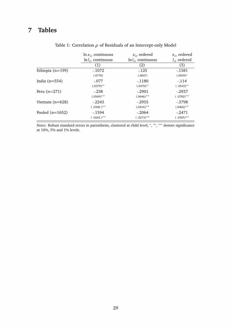
7 Tables

Table 1: Correlation ρ of Residuals of an Intercept-only Model

ln x i t continuous x i t ordered x i t orderedln li t continuous ln li t continuous li t ordered

(1) (2) (3)Ethiopia (n=199) -.1072 -.125 -.1581

(.0778) (.0847) (.0939)∗

India (n=554) -.077 -.1180 -.114(.0379)∗∗ (.0470)∗∗ ( .0543)∗∗

Peru (n=271) -.238 -.2901 -.2937(.0569)∗∗∗ (.0646)∗∗∗ ( .0782)∗∗∗

Vietnam (n=628) -.2243 -.2955 -.3798( .0346 )∗∗∗ (.0416)∗∗∗ (.0466)∗∗∗

Pooled (n=1652) -.1594 -.2064 -.2471( .0242 )∗∗∗ ( .0273)∗∗∗ ( .0305)∗∗∗

Notes: Robust standard errors in parenthesis, clustered at child level; ∗, ∗∗, ∗∗∗ denote significanceat 10%, 5% and 1% levels.

29

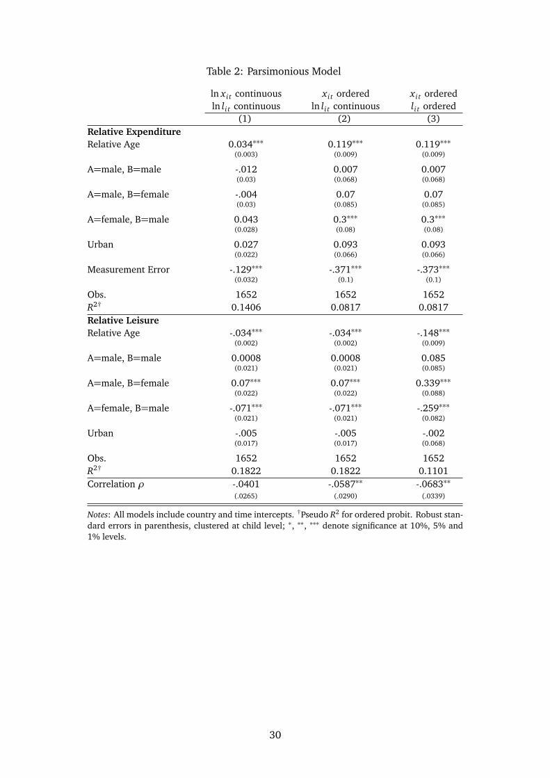
Table 2: Parsimonious Model

ln x i t continuous x i t ordered x i t orderedln li t continuous ln li t continuous li t ordered

(1) (2) (3)Relative ExpenditureRelative Age 0.034∗∗∗ 0.119∗∗∗ 0.119∗∗∗

(0.003) (0.009) (0.009)

A=male, B=male -.012 0.007 0.007(0.03) (0.068) (0.068)

A=male, B=female -.004 0.07 0.07(0.03) (0.085) (0.085)

A=female, B=male 0.043 0.3∗∗∗ 0.3∗∗∗(0.028) (0.08) (0.08)

Urban 0.027 0.093 0.093(0.022) (0.066) (0.066)

Measurement Error -.129∗∗∗ -.371∗∗∗ -.373∗∗∗(0.032) (0.1) (0.1)

Obs. 1652 1652 1652R2† 0.1406 0.0817 0.0817Relative LeisureRelative Age -.034∗∗∗ -.034∗∗∗ -.148∗∗∗

(0.002) (0.002) (0.009)

A=male, B=male 0.0008 0.0008 0.085(0.021) (0.021) (0.085)

A=male, B=female 0.07∗∗∗ 0.07∗∗∗ 0.339∗∗∗(0.022) (0.022) (0.088)

A=female, B=male -.071∗∗∗ -.071∗∗∗ -.259∗∗∗(0.021) (0.021) (0.082)

Urban -.005 -.005 -.002(0.017) (0.017) (0.068)

Obs. 1652 1652 1652R2† 0.1822 0.1822 0.1101Correlation ρ -.0401 -.0587∗∗ -.0683∗∗

(.0265) (.0290) (.0339)

Notes: All models include country and time intercepts. †Pseudo R2 for ordered probit. Robust stan-dard errors in parenthesis, clustered at child level; ∗, ∗∗, ∗∗∗ denote significance at 10%, 5% and1% levels.

30

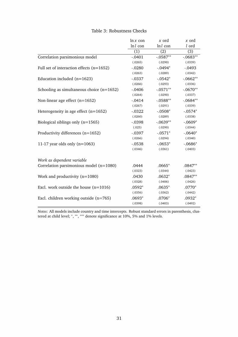
Table 3: Robustness Checks

ln x con x ord x ordln l con ln l con l ord

(1) (2) (3)Correlation parsimonious model -.0401 -.0587∗∗ -.0683∗∗

(.0265) (.0290) (.0339)

Full set of interaction effects (n=1652) -.0280 -.0494∗ -.0493(.0263) (.0289) (.0342)

Education included (n=1623) -.0337 -.0542∗ -.0662∗∗

(.0266) (.0293) (.0336)

Schooling as simultaneous choice (n=1652) -.0406 -.0571∗∗ -.0670∗∗

(.0264) (.0290) (.0337)

Non-linear age effect (n=1652) -.0414 -.0588∗∗ -.0684∗∗

(.0267) (.0291) (.0339)

Heterogeneity in age effect (n=1652) -.0322 -.0508∗ -.0574∗

(.0260) (.0289) (.0338)

Biological siblings only (n=1565) -.0398 -.0639∗∗ -.0609∗

(.025) (.0290) (.0344)

Productivity differences (n=1652) -.0397 -.0571∗ -.0640∗

(.0266) (.0294) (.0340)

11-17 year olds only (n=1063) -.0538 -.0653∗ -.0686∗

(.0346) (.0361) (.0403)

Work as dependent variableCorrelation parsimonious model (n=1080) .0444 .0665∗ .0847∗∗

(.0323) (.0344) (.0423)

Work and productivity (n=1080) .0430 .0632∗ .0847∗∗

(.0328) (.0406) (.0426)

Excl. work outside the house (n=1016) .0592∗ .0635∗ .0770∗

(.0356) (.0362) (.0442)

Excl. children working outside (n=765) .0693∗ .0706∗ .0932∗

(.0398) (.0403) (.0492)

Notes: All models include country and time intercepts. Robust standard errors in parenthesis, clus-tered at child level; ∗, ∗∗, ∗∗∗ denote significance at 10%, 5% and 1% levels.

31

8 Figures

Figure 1: Unconditional Joint Distribution of ln x i t and ln li t

01

23

4as

inh(

expe

nditu

re)

0 .5 1 1.5 2 2.5asinh(leisure)

Ethiopia

01

23

asin

h(ex

pend

iture

)

0 .5 1 1.5 2 2.5asinh(leisure)

India

01

23

asin

h(ex

pend

iture

)

0 .5 1 1.5 2 2.5asinh(leisure)

Peru0

12

3as

inh(

expe

nditu

re)

0 1 2 3asinh(leisure)

Vietnam

Notes: Y-axis shows relative expenditure using the inverse hyperbolic sine transformation; x-axis showsrelative leisure using the inverse hyperbolic sine transformation. The figure contains circles and hexagons.Circles represent individual data points; in a light hexagon each line from the centre represents one ob-servation; in a dark hexagon, each line from the centre represents four observations; overlaid are a linearregression and a local polynomial regression with 95% confidence intervals.

32

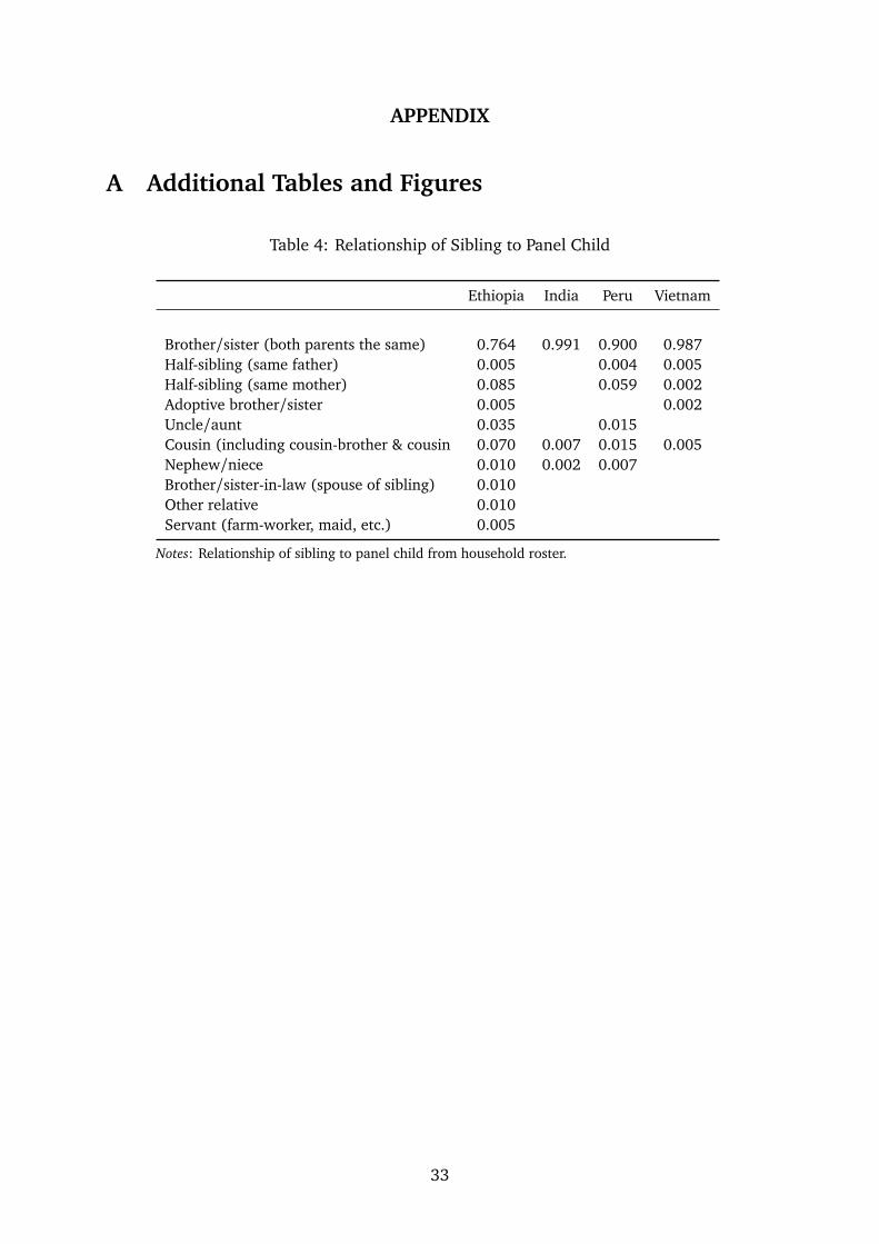
APPENDIX

A Additional Tables and Figures

Table 4: Relationship of Sibling to Panel Child

Ethiopia India Peru Vietnam

Brother/sister (both parents the same) 0.764 0.991 0.900 0.987Half-sibling (same father) 0.005 0.004 0.005Half-sibling (same mother) 0.085 0.059 0.002Adoptive brother/sister 0.005 0.002Uncle/aunt 0.035 0.015Cousin (including cousin-brother & cousin 0.070 0.007 0.015 0.005Nephew/niece 0.010 0.002 0.007Brother/sister-in-law (spouse of sibling) 0.010Other relative 0.010Servant (farm-worker, maid, etc.) 0.005

Notes: Relationship of sibling to panel child from household roster.

33

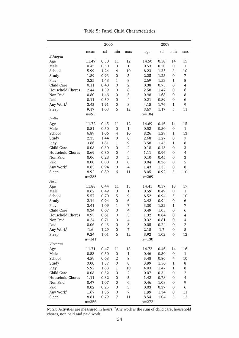
Table 5: Panel Child Characteristics

2006 2009

mean sd min max age sd min maxEthiopiaAge 11.49 0.50 11 12 14.50 0.50 14 15Male 0.45 0.50 0 1 0.53 0.50 0 1School 5.99 1.24 4 10 6.23 1.35 3 10Study 1.89 0.93 0 5 2.25 1.23 0 7Play 3.25 1.48 1 8 2.69 1.53 1 8Child Care 0.11 0.40 0 2 0.38 0.75 0 4Household Chores 2.44 1.59 0 8 2.58 1.47 0 6Non Paid 0.80 1.46 0 5 0.98 1.68 0 8Paid 0.11 0.59 0 4 0.21 0.89 0 6Any Work† 3.45 1.91 0 8 4.15 1.76 1 9Sleep 9.17 1.03 6 12 8.67 1.17 5 11

n=95 n=104IndiaAge 11.72 0.45 11 12 14.69 0.46 14 15Male 0.51 0.50 0 1 0.52 0.50 0 1School 6.89 1.06 4 10 8.26 1.29 1 13Study 2.33 1.44 0 8 2.68 1.27 0 7Play 3.86 1.81 1 9 3.58 1.45 1 8Child Care 0.08 0.30 0 2 0.18 0.43 0 3Household Chores 0.69 0.80 0 4 1.11 0.96 0 4Non Paid 0.06 0.28 0 3 0.10 0.45 0 3Paid 0.00 0.00 0 0 0.04 0.36 0 5Any Work† 0.83 0.94 0 4 1.43 1.35 0 8Sleep 8.92 0.89 6 11 8.05 0.92 5 10

n=285 n=269PeruAge 11.88 0.44 11 13 14.41 0.57 13 17Male 0.62 0.49 0 1 0.59 0.49 0 1School 5.57 0.70 5 9 6.52 0.94 5 10Study 2.14 0.94 0 6 2.42 0.94 0 6Play 2.41 1.09 1 7 3.30 1.32 1 7Child Care 0.34 0.67 0 4 0.49 1.05 0 6Household Chores 0.95 0.61 0 3 1.32 0.84 0 4Non Paid 0.24 0.71 0 4 0.32 0.81 0 4Paid 0.06 0.43 0 3 0.05 0.24 0 2Any Work† 1.6 1.29 0 7 2.18 1.7 0 8Sleep 9.24 1.01 6 12 8.92 1.02 6 12

n=141 n=130VietnamAge 11.71 0.47 11 13 14.72 0.46 14 16Male 0.53 0.50 0 1 0.46 0.50 0 1School 4.59 0.63 2 8 5.48 0.86 4 10Study 3.00 1.57 0 8 3.99 1.56 1 8Play 5.92 1.83 1 10 4.03 1.47 1 8Child Care 0.08 0.32 0 2 0.07 0.34 0 2Household Chores 1.11 0.82 0 5 1.42 0.78 0 4Non Paid 0.47 1.07 0 6 0.46 1.08 0 9Paid 0.02 0.25 0 3 0.03 0.37 0 6Any Work† 1.67 1.36 0 7 1.99 1.34 0 11Sleep 8.81 0.79 7 11 8.54 1.04 5 12

n=356 n=272

Notes: Activities are measured in hours; †Any work is the sum of child care, householdchores, non paid and paid work.

34

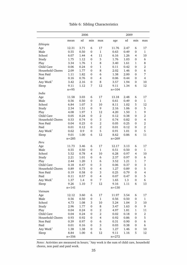
Table 6: Sibling Characteristics

2006 2009

mean sd min max age sd min maxEthiopiaAge 12.31 3.71 6 17 11.76 2.47 6 17Male 0.55 0.50 0 1 0.63 0.49 0 1School 6.07 1.44 4 11 6.16 1.26 4 10Study 1.75 1.12 0 5 1.76 1.03 0 6Play 3.34 1.76 1 8 3.40 1.61 1 8Child Care 0.06 0.24 0 1 0.11 0.42 0 2Household Chores 2.09 1.77 0 8 2.02 1.46 0 6Non Paid 1.11 1.82 0 6 1.38 2.00 0 7Paid 0.16 0.76 0 4 0.06 0.44 0 4Any Work† 3.42 2.16 0 8 3.57 1.94 0 10Sleep 9.11 1.12 7 12 9.11 1.34 6 12

n=95 n=104IndiaAge 11.58 3.03 6 17 13.18 2.48 6 17Male 0.56 0.50 0 1 0.61 0.49 0 1School 6.84 1.07 3 10 8.11 1.02 5 12Study 2.34 1.51 0 9 2.16 1.06 0 5Play 4.08 1.97 1 12 4.20 1.50 1 9Child Care 0.05 0.24 0 2 0.12 0.38 0 2Household Chores 0.53 0.74 0 3 0.74 0.82 0 4Non Paid 0.04 0.23 0 2 0.05 0.25 0 2Paid 0.01 0.12 0 2 0.01 0.12 0 2Any Work† 0.62 0.9 0 5 0.91 1.01 0 5Sleep 9.01 1.00 6 12 8.62 0.86 6 11

n=285 n=269PeruAge 11.73 3.46 6 17 12.17 3.13 6 17Male 0.55 0.50 0 1 0.51 0.50 0 1School 5.52 0.78 4 10 6.28 0.97 4 10Study 2.21 1.01 0 6 2.37 0.97 0 6Play 2.44 1.20 1 6 3.52 1.21 1 7Child Care 0.18 0.47 0 3 0.06 0.37 0 3Household Chores 0.89 0.73 0 4 1.27 0.89 0 5Non Paid 0.19 0.58 0 3 0.25 0.79 0 4Paid 0.11 0.57 0 4 0.07 0.47 0 5Any Work† 1.37 1.4 0 7 1.65 1.3 0 6Sleep 9.26 1.10 7 12 9.16 1.11 6 13

n=141 n=130VietnamAge 12.12 3.60 6 17 11.97 3.54 6 17Male 0.56 0.50 0 1 0.56 0.50 0 1School 4.73 1.08 3 10 5.24 1.04 3 10Study 2.96 1.77 0 8 3.47 1.63 0 9Play 0.04 0.24 0 2 4.97 1.81 1 11Child Care 0.04 0.24 0 2 0.02 0.18 0 2Household Chores 0.93 0.92 0 4 0.92 0.86 0 5Non Paid 0.39 0.97 0 6 0.31 0.90 0 6Paid 0.01 0.16 0 3 0.03 0.38 0 6Any Work† 1.38 1.38 0 6 1.27 1.46 0 10Sleep 8.84 1.00 6 12 9.11 1.16 5 12

n=356 n=272

Notes: Activities are measured in hours; †Any work is the sum of child care, householdchores, non paid and paid work.

35

Table 7: Clothes Expenditure per Child

Ethiopia 2006 2009

mean sd min max mean sd min maxEthiopiaIndex ChildClothes 75.9 52.5 7.5 337.5 164.9 166.3 4.25 1000male 72.0 50.7 7.5 235 151.9 121.1 4.25 600female 79.2 54.3 19 337.5 179.4 206.0 25 1000

SiblingClothes 112.3 114.2 2.5 640 159.7 158.9 12.75 750male 123.2 134.2 2.5 640 169.2 161.3 12.75 710female 99.2 83.6 5 400 143.9 155.7 20 750

IndiaIndex ChildClothes 584.1 424.8 50 2500 1104.4 1133.6 100 13500male 603.5 412.3 120 2500 1072.9 666.3 200 5000female 564.3 437.7 50 2500 1138.6 1485.4 100 13500

SiblingClothes 655.0 550.9 60 5000 1285.7 1287.4 50 15000male 584.5 538.7 60 5000 1260.8 1027.2 50 8000female 745.2 555.3 100 3000 1325.3 1621.8 100 15000

PeruIndex ChildClothes 106.2 91.1 6 750 162.4 201.8 8 1300male 104.3 73.2 6 300 157.8 218.6 8 1300female 109.1 114.9 20 750 169.0 176.5 10 1000

SiblingClothes 108.2 90.6 9 525 138.7 156.1 8 1000male 107.7 95.6 15 525 161.4 244.0 15 1500female 108.7 85.0 9 500 149.9 203.7 8 1500

VietnamIndex ChildClothes 198.4 189.9 15 2000 489.4 790.4 20 10000male 180.6 151.9 45 1500 489.9 712.1 37.5 7000female 218.6 224.2 15 2000 488.9 854.7 20 10000

SiblingClothes 212.0 231.7 15 3000 408.7 767.7 12.5 10000male 220.8 284.8 15 3000 383.6 613.4 12.5 7000female 200.5 135.0 30 750 440.2 926.7 20 10000

Notes: Measured in local currencies.

36

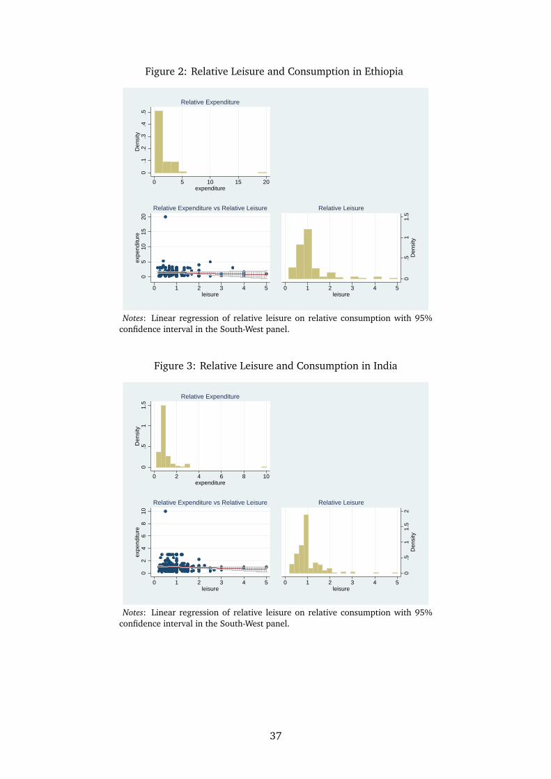
Figure 2: Relative Leisure and Consumption in Ethiopia

0.1

.2.3

.4.5

Den

sity

0 5 10 15 20expenditure

Relative Expenditure

05

1015

20ex

pend

iture

0 1 2 3 4 5leisure

Relative Expenditure vs Relative Leisure

0.5

11.

5D

ensi

ty

0 1 2 3 4 5leisure

Relative Leisure

Notes: Linear regression of relative leisure on relative consumption with 95%confidence interval in the South-West panel.

Figure 3: Relative Leisure and Consumption in India

0.5

11.

5D

ensi

ty

0 2 4 6 8 10expenditure

Relative Expenditure

02

46

810

expe

nditu

re

0 1 2 3 4 5leisure

Relative Expenditure vs Relative Leisure

0.5

11.

52

Den

sity

0 1 2 3 4 5leisure

Relative Leisure

Notes: Linear regression of relative leisure on relative consumption with 95%confidence interval in the South-West panel.

37

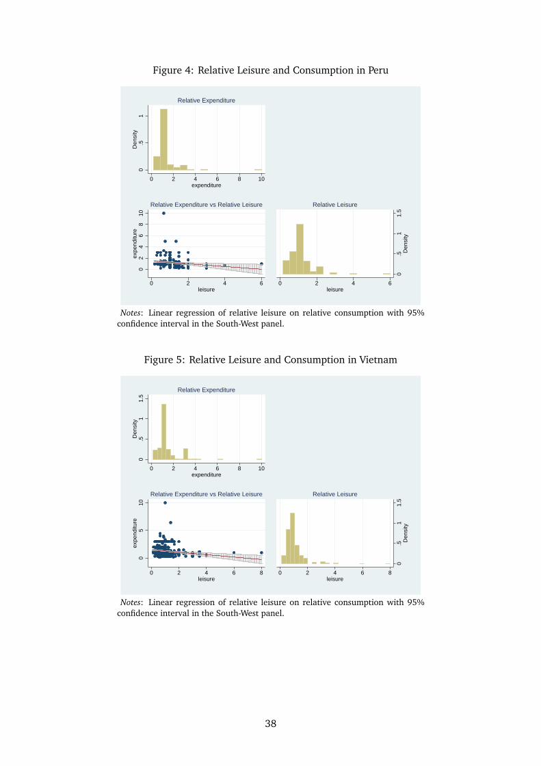
Figure 4: Relative Leisure and Consumption in Peru

0.5

1D

ensi

ty

0 2 4 6 8 10expenditure

Relative Expenditure

02

46

810

expe

nditu

re

0 2 4 6leisure

Relative Expenditure vs Relative Leisure

0.5

11.

5D

ensi

ty

0 2 4 6leisure

Relative Leisure

Notes: Linear regression of relative leisure on relative consumption with 95%confidence interval in the South-West panel.

Figure 5: Relative Leisure and Consumption in Vietnam

0.5

11.

5D

ensi

ty

0 2 4 6 8 10expenditure

Relative Expenditure

05

10ex

pend

iture

0 2 4 6 8leisure

Relative Expenditure vs Relative Leisure

0.5

11.

5D

ensi

ty

0 2 4 6 8leisure

Relative Leisure

Notes: Linear regression of relative leisure on relative consumption with 95%confidence interval in the South-West panel.

38

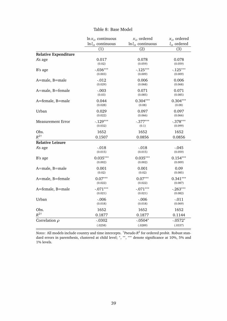
Table 8: Base Model

ln x i t continuous x i t ordered x i t orderedln li t continuous ln li t continuous li t ordered

(1) (2) (3)Relative ExpenditureA’s age 0.017 0.078 0.078

(0.02) (0.059) (0.059)

B’s age -.036∗∗∗ -.125∗∗∗ -.125∗∗∗(0.003) (0.009) (0.009)

A=male, B=male -.012 0.006 0.006(0.029) (0.068) (0.068)

A=male, B=female -.003 0.071 0.071(0.03) (0.085) (0.085)

A=female, B=male 0.044 0.304∗∗∗ 0.304∗∗∗(0.028) (0.08) (0.08)

Urban 0.029 0.097 0.097(0.022) (0.066) (0.066)

Measurement Error -.129∗∗∗ -.377∗∗∗ -.378∗∗∗(0.032) (0.1) (0.099)

Obs. 1652 1652 1652R2† 0.1507 0.0856 0.0856Relative LeisureA’s age -.018 -.018 -.045

(0.015) (0.015) (0.059)

B’s age 0.035∗∗∗ 0.035∗∗∗ 0.154∗∗∗(0.002) (0.002) (0.009)

A=male, B=male 0.001 0.001 0.09(0.02) (0.02) (0.085)

A=male, B=female 0.07∗∗∗ 0.07∗∗∗ 0.341∗∗∗(0.022) (0.022) (0.087)

A=female, B=male -.071∗∗∗ -.071∗∗∗ -.263∗∗∗(0.021) (0.021) (0.082)

Urban -.006 -.006 -.011(0.018) (0.018) (0.069)

Obs. 1652 1652 1652R2† 0.1877 0.1877 0.1144Correlation ρ -.0302 -.0504∗ -.0572∗

(.0258) (.0289) (.0337)

Notes: All models include country and time intercepts. †Pseudo R2 for ordered probit. Robust stan-dard errors in parenthesis, clustered at child level; ∗, ∗∗, ∗∗∗ denote significance at 10%, 5% and1% levels.

39

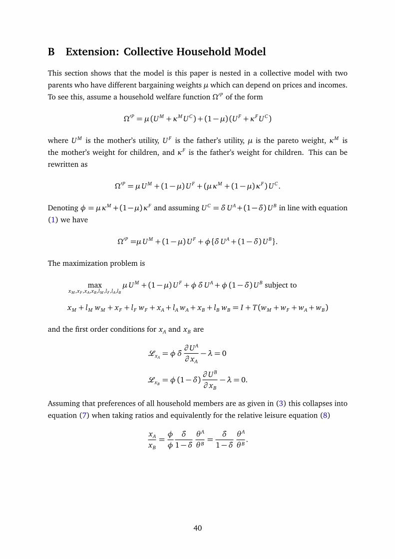
B Extension: Collective Household Model

This section shows that the model is this paper is nested in a collective model with two

parents who have different bargaining weights µ which can depend on prices and incomes.

To see this, assume a household welfare function Ω′P of the form

Ω′P = µ (U M + κM UC) + (1−µ) (U F +κF UC)

where U M is the mother’s utility, U F is the father’s utility, µ is the pareto weight, κM is

the mother’s weight for children, and κF is the father’s weight for children. This can be

rewritten as

Ω′P = µU M + (1−µ)U F + (µκM + (1−µ)κF)UC .

Denoting φ = µκM +(1−µ)κF and assuming UC = δUA+(1−δ)UB in line with equation

(1) we have

Ω′P =µU M + (1−µ)U F +φδUA+ (1−δ)UB.

The maximization problem is

maxxM ,xF ,xA,xB ,lM ,lF ,lA,lB

µU M + (1−µ)U F +φδUA+φ (1−δ)UB subject to

xM + lM wM + xF + lF wF + xA+ lA wA+ xB + lB wB = I + T (wM +wF +wA+wB)

and the first order conditions for xA and xB are

LxA= φδ

∂ UA

∂ xA−λ= 0

LxB= φ (1−δ)

∂ UB

∂ xB−λ= 0.

Assuming that preferences of all household members are as given in (3) this collapses into

equation (7) when taking ratios and equivalently for the relative leisure equation (8)

xA

xB=φ

φ

δ

1−δθA

θ B=

δ

1−δθA

θ B.

40

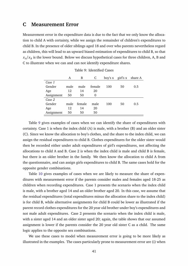
C Measurement Error

Measurement error in the expenditure data is due to the fact that we only know the alloca-

tion to child A with certainty, while we assign the remainder of children’s expenditures to

child B. In the presence of older siblings aged 18 and over who parents nevertheless regard

as children, this will lead to an upward biased estimation of expenditures to child B, so that

xA/xB is the lower bound. Below we discuss hypothetical cases for three children, A, B and

C to illustrate when we can and can not identify expenditure shares.

Table 9: Identified Cases

A B C boy’s x girl’s x share ACase 1Gender male male female 100 50 0.5Age 12 14 20Assignment 50 50 0Case 2Gender male female male 100 50 0.5Age 12 14 20Assignment 50 50 50

Table 9 gives examples of cases when we can identify the share of expenditures with

certainty. Case 1 is when the index child (A) is male, with a brother (B) and an older sister

(C). Since we know the allocation to boy’s clothes, and the share to the index child, we can

assign the residual expenditures to child B. Clothes expenditures for the older sister would

then be recorded either under adult expenditures of girl’s expenditures, not affecting the

allocations to child A and B. Case 2 is when the index child is male and child B is female,

but there is an older brother in the family. We then know the allocation to child A from

the questionnaire, and can assign girls expenditures to child B. The same cases hold for the

opposite gender combinations.

Table 10 gives examples of cases when we are likely to measure the share of expen-

ditures with measurement error if the parents consider males and females aged 18-25 as

children when recording expenditures. Case 1 presents the scenario when the index child

is male, with a brother aged 14 and an older brother aged 20. In this case, we assume that

the residual expenditures (total expenditures minus the allocation share to the index child)

is for child B, while alternative assignments for child B could be lower as illustrated if the

parent record clothes expenditures for the 20 year old brother under boy’s expenditures and

not male adult expenditures. Case 2 presents the scenario when the index child is male,

with a sister aged 14 and an older sister aged 20; again, the table shows that our assumed

assignment is lower if the parents consider the 20 year old sister C as a child. The same

logic applies to the opposite sex combinations.

We use these cases to model when measurement error is going to be more likely as

illustrated in the examples. The cases particularly prone to measurement error are (i) when

41

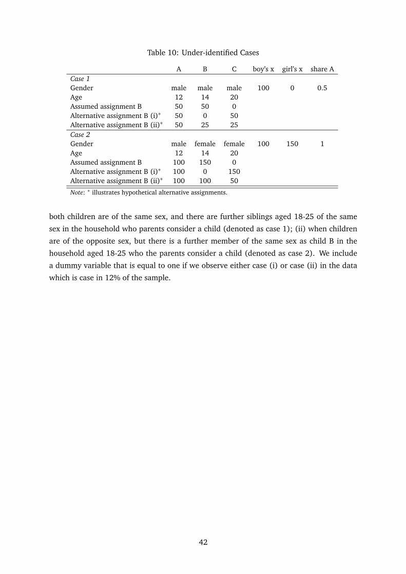
Table 10: Under-identified Cases

A B C boy’s x girl’s x share ACase 1Gender male male male 100 0 0.5Age 12 14 20Assumed assignment B 50 50 0Alternative assignment B (i)∗ 50 0 50Alternative assignment B (ii)∗ 50 25 25Case 2Gender male female female 100 150 1Age 12 14 20Assumed assignment B 100 150 0Alternative assignment B (i)∗ 100 0 150Alternative assignment B (ii)∗ 100 100 50

Note: ∗ illustrates hypothetical alternative assignments.

both children are of the same sex, and there are further siblings aged 18-25 of the same

sex in the household who parents consider a child (denoted as case 1); (ii) when children

are of the opposite sex, but there is a further member of the same sex as child B in the

household aged 18-25 who the parents consider a child (denoted as case 2). We include

a dummy variable that is equal to one if we observe either case (i) or case (ii) in the data

which is case in 12% of the sample.

42