PREFACE - Universiteit Hasselt · PREFACE The master thesis ... Moreover, the annual report...
87
PREFACE The master thesis is the final part of the Master Program of Transportation Sciences at Hasselt University, in which students have to implement all the knowledge they gathered during the two years of studying. The topic of this thesis was chosen in order to expand my knowledge in traffic modelling, which is a useful practice that is frequently used in many transportation planning companies all over the world. I would like to thank my promoter prof. dr. ir. Tom Bellemans for always being able and willing to help me. Many thanks go out to my supervisor Jan Vuurstaek, for his guidance, help and interest shown in my research. I would also like to thank him for his ability to answer all the questions I had. I especially want to thank ir. Luk Knapen for his help, enthusiasm, knowledge and experience in the transportation behavior sciences, which he shared. His supervision allowed my research to be interesting and comfortable. Most thanks go out to my family and friends, who supported me in writing this thesis and during two years I studied at the university and spent in Belgium. I appreciate that I have all of you in my life. Julia Naumova Master student of Transportation Sciences, January 2016
Transcript of PREFACE - Universiteit Hasselt · PREFACE The master thesis ... Moreover, the annual report...

PREFACE
The master thesis is the final part of the Master Program of Transportation
Sciences at Hasselt University, in which students have to implement all the
knowledge they gathered during the two years of studying. The topic of this
thesis was chosen in order to expand my knowledge in traffic modelling, which
is a useful practice that is frequently used in many transportation planning
companies all over the world.
I would like to thank my promoter prof. dr. ir. Tom Bellemans for always being
able and willing to help me.
Many thanks go out to my supervisor Jan Vuurstaek, for his guidance, help and
interest shown in my research. I would also like to thank him for his ability to
answer all the questions I had.
I especially want to thank ir. Luk Knapen for his help, enthusiasm, knowledge
and experience in the transportation behavior sciences, which he shared. His
supervision allowed my research to be interesting and comfortable.
Most thanks go out to my family and friends, who supported me in writing this
thesis and during two years I studied at the university and spent in Belgium. I
appreciate that I have all of you in my life.
Julia Naumova
Master student of Transportation Sciences, January 2016

Building traffic models using freely available data | 2

A case study in Leuven | 3
SUMMARY
This master thesis is aimed at building a traffic model for the region of Leuven,
which ficuses on the traffic generated by the University Hospitals. The model is
aimed at public transport flow predictions, which could aid in the further
development of public transportation systems and urban planning in the future.
Building a traffic model needs operating a traffic simulator, which in this thesis
was MATSim.
The first part of this master thesis consists of a literature study, which focused
on understanding the main principles of building traffic models: their types,
structure, methods of data collection, strengths and weaknesses.
Besides the literature study, the first phase of research included the hospital-
related data collection - which, along with the synthetic plans derived from
FEATHERS, will become components that will be included into the traffic model.
The case study is an activity-based model and therefore has a time-dependent
character. However, the data regarding to the University Hospitals of Leuven
included the time-dependent information about the distribution of the hospital
visitors throughout the day. To collect the information concerning the
distribution, all those people who visited the hospitals have been divided into the
following three main categories:
Patients
Visitors of patients
Personnel
The average number of consultations on a workday, the single-day and multi-day
hospitalizations and the number of beds found in the annual report (Guy
Mannaerts, 2013), allowed to identify the average number of patients that visited
the hospitals every day in 2013.
Based on the average number of trips made by one patient per day, rules
regarding visiting patients found in the literature and data from the official
hospital website (“UZ Leuven - Universitair ziekenhuis,” 2014), the daily
distribution of visitors could be created.
To identify the daily personnel distribution, the total number of employees has
been divided into the following categories:
Doctors
Nurses
Remaining shift staff
Remaining office hours staff
The information related to the hospital - doctors‟ working hours (from 8h30 till
17h30), the list of doctors found on the hospitals website, allowed to find how
many and when doctors arrived and left the hospitals during a single day.

Building traffic models using freely available data | 4
The number of nurses has been calculated by multiplying the number of beds by
the average amount of nurses needed per day per bed. This amount is identified
by the hospitals nursing workforce calculation technique created by J. M. Welton
(2011). For the nurses category, which, according to the same author, consists
of complete shift employees, the hospitals have set shifts with specific start and
end times:
6h00-14h00
14h00-22h00
22h00-6h00
The other remaining personnel is assumed to be composed of 10% shifts workers
(“Vlaamse statistieken,” 2014), who work the same hours as nurses do, and
90% office hours staff working regular hours.
Moreover, the annual report provided the information concerning the mode
choice of personnel of the Gasthuisberg campus. It was found that 14% of the
personnel commuted by public transport, 57% of the staff preferred travelling by
car (Jan Paesen, 2011), 15% of staff were car passengers and the remaining
14% were vulnerable road users (cyclists and pedestrians). In this thesis, the
mode choice per personnel category has been calculated by multiplying the
number of employees with the percentage of commuters mentioned earlier.
Finally, according to the master thesis topic, the data mentioned above has been
collected using freely available sources, which did not demand special access to
acquire.
The second part of the research is aimed at the simulation of the built traffic
model using MATSim, in which the gathered hospital-related data and FEATHERS
synthetic plans served as two kinds of inputs (along with other inputs, such as
PT-schedules, population, network and facilities). From the outputs of this
simulation, which consisted of event logs, information about buses have to be
extracted and converted into the bus-line profiles by the research group of
transportation behaviour at the transportation research institute at Hasselt
University.
The third part has to evaluate the quality of the built model by comparison of the
bus-line profiles obtained during this master thesis and the ones provided by the
Belgian bus company „De Lijn‟. A large number of similarities between
corresponding profiles (e.g. approximately the same number of passengers
alighting at the same bus stop) has to indicate that the built traffic model, based
on the open source data obtained during the first stage of the research, has
enough power to predict public transport flows in the future.
Keywords demand prediction, freely available data, MATSim, public transport,
traffic modelling

A case study in Leuven | 5
TABLE OF CONTENT
PREFACE ................................................................................................... 1
SUMMARY ................................................................................................. 3
TABLE OF CONTENT .................................................................................... 5
LIST OF FIGURES ....................................................................................... 7
LIST OF TABLES ......................................................................................... 8
1. INTRODUCTION ............................................................................... 11
2. OUTLINE THESIS ............................................................................. 13
2.1 Data collection .............................................................................. 13
2.2 Simulation .................................................................................... 14
2.3 Comparing bus-line profiles ............................................................ 15
2.4 Objective ..................................................................................... 17
2.5 Research questions ....................................................................... 18
3. LITERATURE STUDY ......................................................................... 21
3.1 SMART-PT .................................................................................... 21
3.2 Traffic modelling ........................................................................... 21
3.2.1 Four-step model ...................................................................... 23
3.2.2 Activity-based models .............................................................. 25
3.2.3 ALBATROSS ............................................................................ 28
3.2.4 FEATHERS .............................................................................. 29
4. UNIVERSITY HOSPITALS-RELATED DATA COLLECTION ......................... 31
4.1 Daily basis ................................................................................... 32
4.2 The Gasthuisberg campus .............................................................. 34
4.2.1 Mode choice ............................................................................ 36
4.3 Pellenberg campus ........................................................................ 37
4.4 Sint-Rafael and Sint-Pieter campus ................................................. 38
5. SIMULATION ................................................................................... 41

Building traffic models using freely available data | 6
5.1 MATSim software, overview ............................................................ 41
5.2 Data requirements ........................................................................ 42
5.2.1 Configuration file (config.xml) ................................................... 43
5.2.2 Population file (plans.xml) ........................................................ 46
5.2.3 Network file (network.xml) ....................................................... 47
5.3 Public transport simulation in MATSim ............................................. 48
5.3.1 Schedule file (schedule.xml) ..................................................... 48
5.3.2 Vehicles file (vehicles.xml) ........................................................ 50
5.4 Testing of small scenarios .............................................................. 51
5.4.1 Simulating different modes ....................................................... 51
5.4.2 Simulating walking .................................................................. 59
5.4.3 Switching two buses ................................................................ 60
5.4.4 Simulating multi-modal trips ..................................................... 62
5.4.5 Network with link length zero included ....................................... 63
5.4.6 Network with the low capacity link included ................................ 65
5.5 Leuven scenario ............................................................................ 68
CONCLUSION ........................................................................................... 75
DISCUSSION ........................................................................................... 79
REFERENCES ........................................................................................... 81

A case study in Leuven | 7
LIST OF FIGURES
Figure 1 Location of Leuven railway station and hospital campuses on the map
.............................................................................................................. 12
Figure 2 Research methodology ................................................................ 13
Figure 3 The Gasthuisberg campus showed on the map .............................. 15
Figure 4 Example of event log, MATSim output ........................................... 15
Figure 5 Bus-line profile ........................................................................... 16
Figure 6 MATSim basic structure .............................................................. 18
Figure 7 Process of traffic modelling ......................................................... 22
Figure 8 The four-step model ................................................................... 23
Figure 9 An example of how trips are modeled in a four-step model .............. 24
Figure 10 Representation of linkage between activities‟ in activity-based model
.............................................................................................................. 27
Figure 11 FEATHERS‟ input and output data .............................................. 30
Figure 12 Building blocks in MATSim ........................................................ 41
Figure 13 Network #1 ............................................................................. 51
Figure 14 Network #1. Long home and work location parts .......................... 52
Figure 15 Network #1. Short home and work location parts ......................... 53
Figure 16 Example of a U-turn .................................................................. 56
Figure 17 Network #1. Bus station in the form of circle ............................... 58
Figure 18 Network #2 ............................................................................. 59
Figure 19 Network #3 ............................................................................. 60
Figure 20 Network #4 ............................................................................. 62
Figure 21 Network #5 ............................................................................. 63
Figure 22 Network #6 ............................................................................. 65
Figure 23 Leuven city center with suburbs ................................................. 69
Figure 24 Leuven city center .................................................................... 72

Building traffic models using freely available data | 8
LIST OF TABLES
Table 1 List of objectives for every research step ........................................ 17
Table 2 Examples of software packages .................................................... 22
Table 3 The calculation of the simultaneously and not simultaneously active
personnel ................................................................................................ 34
Table 4 The number of personnel per year for the Gasthuisberg campus ........ 35
Table 5 The number of hospitalizations in the Gasthuisberg campus .............. 35
Table 6 The calculation of the simultaneously and not simultaneously active
personnel in the Gasthuisberg campus ........................................................ 36
Table 7 Daily commuting of the simultaneously active Gasthuisberg personnel 36
Table 8 Daily commuting of not simultaneously active Gasthuisberg personnel 37
Table 9 The number of personnel per year for the Pellenberg campus ............ 37
Table 10 The total number of hospitalizations in the Pellenberg campus ......... 38
Table 11 The calculation of the simultaneously and not simultaneously active
personnel in the Pellenberg campus ............................................................ 38
Table 12 The number of personnel per year for the Sint-Rafael and Sint-Pieter
campus ................................................................................................... 39
Table 13 The total number of hospitalizations in the Sint-Rafael and Sint-Pieter
campuses ................................................................................................ 39
Table 14 The calculation of the simultaneously and not simultaneously active
personnel in the Sint-Rafael and Sint-Pieter campuses .................................. 39
Table 15 Distribution of arriving and leaving Gasthuisberg personnel by mode 40
Table 16 Event logs produced after two simulations .................................... 54
Table 17 Network #1. Results/car ............................................................. 55
Table 18 Network #1. Results/bike............................................................ 56
Table 19 Results/U-turns test ................................................................... 57
Table 20 Event logs. Simulation with U-form bus stations included into the
network .................................................................................................. 58
Table 21 Network #2. Results................................................................... 60
Table 22 Network #3. Results................................................................... 61
Table 23 Network #4. Results................................................................... 62
Table 24 Network #5. Results................................................................... 63
Table 25 Network #6. Results/car ............................................................. 66

A case study in Leuven | 9
Table 26 Network #6. Results/bike ........................................................... 67
Table 27 Network #6. Results/bus ............................................................ 67

Building traffic models using freely available data | 10
Code 1 Config.xml ................................................................................... 45
Code 2 Plans.xml ..................................................................................... 47
Code 3 Nodes and links in the network.xml ................................................. 48
Code 4 Schedule.xml ............................................................................... 50
Code 5 Vehicle‟s parameters in vehicles.xml file .......................................... 50

A case study in Leuven | 11
1. INTRODUCTION
It is not a secret that a lot of countries nowadays face the problem of increasing
travel demand. City roads are overcrowded on a daily basis, which leads to
unpleasant consequences for both travelers and the environment, such as air
pollution, congested roads and an unsafe atmosphere in general (Serge
Hoogendoorn & Victor Knoop, 2004). Today, a lot of factors such as growing
population and increasing immigration increases the probability to use private
cars, what definitely leads to more cars on the road, heavy traffic jams and
increased air pollution. Such problems make public transportation an interesting
alternative, since it could save money, has a high capacity and has less
emissions and therefore less impact on peoples‟ health. Governments,
researchers and transportation companies are interested in the prediction of
public transport demand in order to better regulate traffic flows and make public
transportation systems more effective, especially in big cities with intensive
traffic. Moreover, traffic flow control allows governments to avoid expensive, and
in some cases impossible, infrastructural modifications during the urban planning
phase.
To predict traffic flows and public transport demand, stakeholders try to develop
transportation models, which aim is to reflect the real life traffic situation on the
city roads. Besides software and other necessary tools to create such models,
institutions and companies are interested in accurately gathered data, which
plays an important role for further use in model simulating. Moreover, it
influences the performance of the simulations. Researchers use a wide range of
traffic models, but they always follow the idea of gathering the population,
network, plans-related data/information as realistic as possible.
The focus of this thesis is to use freely available data concerning the distribution
of travelers with regard to the University Hospitals of Leuven. Trips made by the
staff, patients and visitors during the day and their mode choice are the points of
interest.
A huge number of scientific papers have been dedicated to the ways and
methods of data collection. The literature shows that interviewing people that
live in the city are the most effective and reliable tool to collect accurate
information (Joe Castiglione, Mark Bradley, & John Gliebe, 2014). Nevertheless,
the topic of this thesis is using freely available data, and not to generate surveys
to gather the necessary data.
The University Hospitals consist of four campuses, spread out over the city. The
Gasthuisberg campus (hospital) is the largest one and located just outside the
ring road, at a distance of four kilometer from the railway station. The smaller
campuses Sint-Pieter and Sint-Rafael, were built less than one kilometer from
each other and are located two kilometers from the train station. Due to the high
demand for hospital services, the travel demand in this area is believed to have a
significant influence on the city traffic. The bus-lines are going through the city

Building traffic models using freely available data | 12
and buses accommodate a lot of passangers from the hospital campus, since 500
hospitalizations are made every day. Therefore, it can be stated that traveling to
this campus is quite influential on the traffic inside of the city. Due to the large
distance between Pellenberg and the station, around eight kilometers, and the
campuses‟ location outside the city center of Leuven, traffic inside this area is
assumed to have a minimal effect on the buses heading towards Pellenberg and
their bus-line profiles. Figure 1 shows the locations of the different campuses.
Figure 1 Location of Leuven railway station and hospital campuses on the map (“Station
Leuven - Google Maps,” n.d.)
This thesis is divided in four main chapters. The first chapter is outline thesis in
which objectives, research questions and detailed structure of the research are
described. The „Literature study‟ contains the theory dedicated to traffic
modelling, its content and the software used to build the models. The third
chapter is dedicated to hospital-related data gathering. All the numbers,
calculations, techniques and other information, which were used to determine the
distribution of people visiting the hospitals are described in this part of the
thesis. Then, the chapter „Simulation‟ focuses on the simulation of the network in
MATSim with full explanations about how it works, what processes happened
inside, what kind of input MATSim required and what kind of output MATSim
provided. Afterwards, conclusions are made and discussed.

A case study in Leuven | 13
2. OUTLINE THESIS
The master thesis is divided in two chapters and spread over the two semesters
of the academic year 2014-2015 and one semester of the academic year 2015-
2016. The first chapter consists of the literature study and hospitals-related data
collection. During this step, the information regarding the amount of people
visiting the hospitals, the time of their arrival, their departure times and
preferred mode choices were collected. This information contributed to the model
creation and its preparation for further network simulation. In the second
chapter, the main goal was to learn how to use the MATSim software. First, some
small networks were generated and then large scenario were simulated. At the
final stage, comparisons of bus-line profiles gathered in this research and given
by De Lijn, were made. Figure 2 shows a schematic of the research methodology.
Figure 2 Research methodology
The following sections give an overview of the stages of this thesis.
2.1 Data collection
The first stage included the collection of hospital-related data that was made
available by the University Hospitals of Leuven. This data included information
about number of personnel, their working hours, arrival and departure times of

Building traffic models using freely available data | 14
visitors, consultations hours and the number of single-day and multi-day
hospitalizations in 2013. The following information was searched for in order to
simulate the traffic generated by the hospitals visitors and make the traffic
model sufficiently powerful for further public transport predictions. To build the
traffic model, which reflects the current situation as close as possible, the
following information was obtained:
How many personnel, patients and visitors do arrive at the hospitals
and how are they distributed over time?
At what time do personnel, patients and visitors leave the hospitals?
How do these people commute?
In order to acquire this data, besides the information provided by the hospitals,
some calculation techniques found in the literature were used. The hospital-
related data and the data produced by FEATHERS schedule predictor, which has
been developed as a framework to improve activity-based models for
transportation demand, play a role of input for the MATSim. Detailed descriptions
of FEATHERS software is discussed in section 3.2.4. FEATHERS is based on the
Onderzoek verplaatsingsgedrag, further abbreviated as OVG (statistics in
Flanders). Travel surveys are needed to generate daily plans. Zone-based
FEATHERS daily plans were disaggregated to street addresses which means that
the activity location zone was replaced by a randomly chosen street address
within that zone. Furthermore, daily plans for hospitals visitors were generated
by sampling individuals from the synthetic population and inserting a hospital
visit into their plans. Examples of such daily plans are:
Home-work-hospital-home
Home-hospital-work-home
Home-work-hospital-leisure-home
Home-family-leisure-hospital-shopping-home etc.
Then, FEATHERS derived daily plans, which were converted into XML files, which
the micro-simulations tool MATSim required.
2.2 Simulation
To run the traffic model, in addition to the previously described inputs (the
hospital visitors distribution throughout the day, the synthetic plans, zoning, PT-
timetable), MATSim also required some transportation and network-related data.
In this case, information concerning stop locations, time tables and other public
transport-related data coded in GTFS format needed to be converted into XML
files (“iRail.be,” n.d.). Moreover, disaggregated locations and BB-zoning (building
block which means one geographical unit level defined by the amount of

A case study in Leuven | 15
population and running time within every block) prepared by the transportation
behavior research group of IMOB (the Transportation Research Institute, Hasselt
University) are considered to complete the network before the simulation.
Particularly, every model demands a network which represents auto, transit,
non-motorized travel routes, distances, travel time and other network-related
attributes that could influence decision making (Joe Castiglione et al., 2014). The
network has been taken from OpenStreetMap (“OpenStreetMap,” 2014,
“OpenStreetMap Wiki,” 2014) and downloaded to MATSim by a master student
during his internship. OpenStreetMap provides geographical network data, such
as roads, trails and railway stations. To see an example, a screenshot of
OpenStreetMap is shown in Figure 3.
Figure 3 The Gasthuisberg campus showed on the map (“OpenStreetMap,” 2014)
The MATSim micro-simulation results in event logs is shown in Figure 4, which
can be characterized as lists of activities that happened during the simulation.
For instance, person with id #1 ends his home activity and enters a vehicle at
26100 sec, what corresponds to 7h15 (one hour contains 3600 seconds and the
simulation starts at 00:00 hours).
Figure 4 Example of event log, MATSim output
Another example is: person with id 25 stepped of bus 601 at the bus stop with id
3426. It can be said that there will be the huge list with lots of activities, but the
last examples are of interest in this master thesis. In other words, the
information regarding buses need to be extracted from every event log.
2.3 Comparing bus-line profiles
The final part of this thesis consists of comparison of bus-line profiles gathered in
this research and delivered by the Belgian bus company „De Lijn‟. For this
reason, event logs extracted from MATSim have to be converted into XML files
what will be done by the transportation behavior research group of IMOB (the
Transportation Research Institute, Hasselt University).
A bus-line profile can be described as a specific graph that indicates how many
passengers get on and off the bus throughout its entire route (Figure 5). After
their generation, the bus-line profiles are analyzed. The y-axis denotes number

Building traffic models using freely available data | 16
of passengers, the x-axis denotes the bus stop id‟s. The green bars indicate how
many people get on the bus, the blue bars how many passengers get off the bus
and the red line indicates how many passengers are on the bus at any moment
during its route.
Figure 5 Bus-line profile
To analyze if the bus-line profiles are of sufficient quality or not, it is necessary
to find similarities or unacceptable differences between them by answering the
following set of questions:
Is the predicted number of passengers entering at a certain bus stop
similar to the observed amount of passengers entering at that stop?
Is the predicted number of passengers leaving the bus at a certain bus
stop similar to the observed amount of passengers leaving the bus at that
stop?
Is the deviation extensive and if so, why?
One possibility of checking if the obtained results are of sufficient quality is to
compare the bus-line profiles provided by „De Lijn‟ with those gathered in this
research. If the predicted bus-line profiles resemble the profiles provided by „De
Lijn‟, the developed traffic model is successful. If differences are observed,
additional questions need to be answered:
Why is the predictive model not succesful in predicting accurate bus-line
profiles?
Does inaccurate data collection at the beginning of the process cause an
insufficient model?

A case study in Leuven | 17
When the model does not seem to be sufficient enough, calibration might be
required. This means that the input data should be checked and, if possible,
modified. One should take into account that the data regarding the simulation of
people‟s activities in Leuven can be affected by the area surrounding the city. For
example, people just passing by the Leuven area can make transit effect on the
bus-line profiles. Finally, the modelling process should be repeated in order to
achieve as similar bus-line profiles as possible, if necessary with modification of
the data.
2.4 Objective
Nowadays, traffic modelling is an important and necessary tool to keep public
transportation systems in congested cities under control (Scott Miller, 2011). As
contribution to the SMART-PT project (see section 3.1), where future public
transportation in the area of Leuven is analyzed (“project_details,” n.d.), this
study focuses on the traffic generated by the visitors of the University Hospitals.
Table 1 shows the set of goals of every research stage.
Table 1 List of objectives for every research step
Phase Goals
data collection
1 Find freely available hospitals-related data 2 Calculate hospitals visitors distribution over a day
3 FEATHERS schedules+hospitals-related data=daily plans
4 Preparation of XML files model simulation
1 Input XML files 2 Run the simulation
3 Get the output (event logs) 4 Extract bus-related information from event logs
comparing bus-line profiles
1 Create bus-line profiles 2 Compare bus-line profiles obtained with the ones delivered by „De Lijn‟
During the first stage of this research, in which the data is collected, it was
important to identify the distribution of the hospitals visitors, in which
information regarding the total number of visitors, time-related information
about visitors arriving and leaving and transport modes visitors use.
In this research to simulate the traffic in Leuven, the MATSim software is used
(“Agent-Based Transport Simulations | MATSim,” 2014). The working process of
this software is depicted in Figure 6. The micro-simulation process consists of the
data input (in the scheme not all the files used in MATSim are depicted. To
overview some more files see Section 5.1), the simulation process and gathering
the outputs.

Building traffic models using freely available data | 18
Figure 6 MATSim basic structure (“Agent-Based Transport Simulations | MATSim,” 2014)
During the final stage of this research, the comparison of the bus-line profiles
plays an important role to determine if calibration is needed or not.
2.5 Research questions
As stated earlier, the study is concerned with obtaining bus-line profiles which
are created by micro-simulation, based on freely available information. The main
goal of this master thesis is formulated as follows:
Building traffic models using freely available data
Since the main goal of this study is to obtain bus-line profiles of high quality, this
research will contribute to the travel estimation of public transport demand in the
city of Leuven. Based on the scientific sources and researchers‟ opinions, further,
importance and benefits to build traffic models were found and explained.
Since, the whole research is divided in different phases, some additional
questions could be asked. For the the data collection stage, at least, the
following questions need to be answered:
Where can the mode choice data of hospital visitors be obtained?
(infrastructure around the hospitals, parking facilities, bus-stop
accessibility)
What are the working hours of the hospitals staff?
What are the visiting hours?
What are the average number of visits per patient per day?
How many hospitalizations do the campuses have in a day?
Where all the data should be found?
What is the quality of the data?

A case study in Leuven | 19
The simulation part of the thesis could have some questions concerning the
principles of the software process. In order to run the simulation properly, some
questions need to be answered:
What kind of input files should be generated?
Which parameters should the configuration file include?
Does the event file have the complete information?
The last stage of the research-the comparison of bus-line profiles with the
generated ones could have the following set of sub-questions, as previously
stated in the methodology (see section 2.3):
Are there similarities between bus-line profiles generated by the
simulation and the bus-line profiles provided by „De Lijn‟?
Is there a big deviation between bus-line profiles generated in this
research and provided by „De Lijn‟?
What causes these differences?
How much influence does the gathered data, from the first phase, has on
the traffic?
Comparison of the bus-line profiles is necessary to evaluate the quality of the
model predictions. Answering the stated sub-questions will help to achieve the
goals at every research stage.

Building traffic models using freely available data | 20

A case study in Leuven | 21
3. LITERATURE STUDY
In order to provide additional information about the importance and goals of
traffic modelling, literature sources have been studied. Most of those dedicated
to traffic modelling contained a description of model types, structure, methods of
data collection for the first input phase, possible software for the traffic model
simulation phase and explanations of output types.
3.1 SMART-PT
This master thesis contributes to the SMART-PT (Smart Adaptive Public
Transport) project, which aims at creating a public transportation system that is
able to adapt itself, based on the changes in travel patterns of its users. The
project recognizes the passengers flows in case of any changes (e.g. growing
population) and estimates them in space and time, to decide how these flow can
be accommodated. Then, those service routes which have a high demand and
those ones which have a lower demand will be transcend to paratransit service.
In this case paratransit is recognized as a special transport services often
provided as a supplement to fixed-route busses and rail systems by public transit
agencies. Afterwards, the slower adapting components such as buses, trams and
LRT (light rail train) will be transcend as well (IMOB, 2014).
To get insight in building traffics, description of the modelling process, its
importance, benefits and disadvantages are described in the next section,
followed by examples of different model types.
3.2 Traffic modelling
The importance of traffic modelling nowadays is shown in many literature
sources. In “Microscopic traffic model for road networks with a representation of
the capacity drop phenomenon at the junctions” (B. Haut, G. Bastin, & Y.
Chitour, 2005), it is said that traffic modelling is a good representation of the
evaluation of a traffic state on a road network, which is necessary for the
analysis of road congestion control strategies.
According to “Modelling transport” (Juan de Dios Ortuzar & Luis G. Willumsen,
2011), several problems with air pollution, road congestion and accidents happen
daily due to the increasing number of cars. Accidents not only deteriorate the
living quality, they also cost the economic systems a lot of money each year.
Traffic modelling is the simulation of transportation systems (roundabouts,
junctions, routes, roads etc.), including the existing network in the region of
interest and observation, socio-demographic situation and peoples‟ behavior.
Modelling should represent the reality as precisely as possible in order to be able
to answer research questions.
Modelling is used to make predictions of traffic and its congestion in case of
different circumstances such as changes in the city layout, the increase of

Building traffic models using freely available data | 22
population, increased number of cars etc. (Scott Miller, 2011). Besides predicting
congestion, modelling also helps to predict CO2 emission and accidents (Davy
Janssens, 2014b).
In addition, traffic modelling allows engineers/researchers to predict queuing
occurrences, their duration and location. Moreover, traffic modelling aims to
support evaluating the methods of road congestion reduction (Serge
Hoogendoorn & Victor Knoop, 2004).
The main core of building traffic models, as most literature shows, consists of
data collection at the first stage; model simulation at the second and output
gathering at the final stage. Figure 7 illustrates the main parts of modelling,
including the simulation and obtaining activity patterns and event logs.
Figure 7 Process of traffic modelling (Davy Janssens, 2014b)
To simulate the model, various traffic modelling software packages exist and are
defined by three different levels (micro, meso and macroscopic), which are
shown in Table 2. Microscopic means that simulation is organized at the city
level: traffic on intersections and road segments can be simulated, mesoscopic
means the area of regions and at the macroscopic level the large networks can
be simulated. The tools related to the macro and mesoscopic levels are
represented here as an example of existing software, in this thesis only the
microsimulation model MATSim is used.
Table 2 Examples of software packages (“Traffic simulation,” 2014)
Level Software
microscopic MATSim
PTV VISSIM
PARAMICS
mesoscopic DYNASMART
DTALite/NeXTA
macroscopic TransCAD
PTV Visum
OmniTRANS
Input (data,
network)
Simulation
Output (activity
patterns, event
logs)
Traffic modelling

A case study in Leuven | 23
Since, the software choice directly depends on which level of traffic model is
needed, starting from the intersection traffic simulation on the microscopic level
finishing by the modelling of traffic of a big networks at the macroscopic level.
As a part of the literature study, to understand the content of the model building,
some different kinds of models are presented and described in this chapter.
3.2.1 Four-step model
Forecasting traffic flows is the main goal of transport modelling. Most models aim
at predicting future traffic, in which factors influencing increasing or decreasing
demand are identified. One of the most known and applied methods to build
traffic models is the traditional four-step model, in which the process of travel
demand is divided in four stages. These stages include the trip generation, the
trip distribution, the mode choice and the route choice (Ahmed, 2012). A
graphical representation of this model is depicted in Figure 8.
Figure 8 The four-step model
Trip generation is based on a zonal network. In every zone it is specified how
much traffic is produced and how much traffic is attracted. Important factors
(variables) influencing this production and attraction can be, the number of
households, the location of hospitals or the number of available vehicles. This list
can be a long. During the second stage, the number of trips produced and
attracted are being linked to each other. Outcomes of the trip distribution phase
include Origin-Destination matrices (OD-matrices), that clearly state how many
persons are traveling from one zone to another. After the trips are distributed on
the network, the third step describes which modes of transport are selected by
the travelers. At this stage OD-matrices are derived to certain modes of
transport. Traffic assignment, or route choice, specifies the different routes that
are taken by the travelers. Based on certain algorithms, for example the least
cost or the shortest path, trips are assigned a certain route on the network.
The total travel demand specified in the stages of trip generation, trip
distribution, mode choice and trip assignments is fixed, with only the route
choice decision to be determined. Most applications of the four-step model
results equilibrated the link between travel times and/or trip distribution models
[1] Trip generation &
attraction
[2] Trip distribution/des
tination
[3] Mode choice/mod-el
split
[4] Route choice/trip assignment

Building traffic models using freely available data | 24
for a second pass (and occasionally more) through the last three steps, but no
formal convergence is guaranteed in most applications.
Literature has shown some disadvantages of the model. First of all, the model is
not able to link different travel decisions that are made within one family. In
many cases, the individual travel behavior significantly influences the entire
network, but the model cannot predict the decisions of an individual traveler.
Four step models cannot make a sequence in travel decisions, which makes it
difficult to take into account the situation where members of one household are
going to work by bus and coming back to home by another mode of transport,
for example the tram (Davy Janssens, n.d.). For better visual understanding of
how this model works, the process of four step models is shown in Figure 9.
Figure shows no start time, duration or end time of an activity because four step
models do not have a time dimension or direction during a trip. It only creates
isolated and independent trips.
Figure 9 An example of how trips are modeled in a four-step model
Daily activities and the transportation network are the data which four step
models need in order to run. Like all other models, four step models demand
data concerning the travel behavior which can be obtained in most cases through
surveying households or acquiring some statistical information. Daily travel plans
and individuals‟ diaries can help to calibrate four step models. In combination
with these diaries, information about the transportation network is needed for
validation of four step models.
Daily households plans (diaries) can provide the following information:
Personal information (age, gender, social status, income, family members,
the number of cars per family, etc.):
who is travelling?

A case study in Leuven | 25
Travel data (e.g. type of trip, origin and destination, duration, sequence of
trips, etc.):
where do people travel to, when, for how long, etc.?
Vehicle data: to develop trip generation, trip distribution and mode choice
levels:
this data contains the information concerning the transport mode that
households use, even though a person uses the public transport-he is
asked to answer which one and how many times per day.
To sum up, four step models require just like other models precise input data.
Despite the fact that four step models do not build individual activity chains, but
only create one agenda per household, FSMs are still frequently used by
transportation companies in order to model the elementary network, predict
travel demand and influence traffic in the way to relief air pollution, car
congestion and other traffic-management related issues.
3.2.2 Activity-based models
There are some techniques that are used for building traffic models according to
individual travel behavior and they are called activity-based models. Following is
a description of models, their nature and an explanation of their benefits and
disadvantages.
Travel demand consists of activities that people usually perform in their lives.
Households and social groups influence travel behavior as well as spatial and
transportation constraints (Davy Janssens, 2014a). Activity-based models predict
the daily plan for each member of the (synthetic) population (UHasselt, 2014).
Synthetic populations in traffic models are individual actors in the form of
households and household members. For each of the households there should be
characteristics like size, income, number of cars and address. Every member of
the household is described by a set of individual characteristics such as sex, age,
religion and work location (Rolf Moeckel & Klaus Spiekerman, 2003).
Activity-based models (ActBMs) focus on the people‟s activities including their
distribution in time. ActBMs describe how people plan their activities by
identification of the following parameters such as:
What type of activities are performed? (e.g. work, shopping, hospitals,
leisure etc.)
Where do these activities take place? (location/address of activities)
When do people perform these activities? (time of the day)
What is the duration of these activities?

Building traffic models using freely available data | 26
Which mode do people choose to go to an activity? (e.g. bike, car, public
transport)
Do people travel in groups?
What is the order of activities? How are they scheduled?
Data collection is the main point for further implementation of the model. Data
collection processes can be based on finding freely-available data, for example
by using the annual reports, or by means of sending questionnaires to
households with a set of questions concerning their daily plans. Information
regarding land use, demographical data and transport network, are required for
model development (Joe Castiglione et al., 2014).
Data collection in activity-based models is primarily based on the activity-based
surveys, which are usually sent out to households in the region of interest.
According to Rye Baerg (2014) the following types of surveys can be used for the
data collection:
Panel surveys
Revealed/stated preference studies
Internet-based surveys
Tool-surveys
The use of global positioning systems (Tom Bellemans et.al., 2010)
Travel survey data is collected in order to develop different models, including
activity-based ones. This data can be used for the estimation and calibration of
models. Literature (Buehler, 2008) showed that in many countries the household
travel survey is one of the main active transportation data collection techniques.
Surveys are used to get the characteristics of different types of trips. For
instance, the National Household Travel Survey (California) asks to mention the
travel purpose, the length of trip and other origin-destination-related questions.
Analysis of all the surveys‟ results collected allows agencies to chain the trips into
tours, to classify the tours and order and convert them into one list of travel
activities for one day.
According to Joe Castiglione (2014), a survey sample should be at least 6,000
households for a medium-to-large region. Since activity-based models require
the collection of variables concerning the socio-economic status and choice
alternatives variables for the respondents, the sample size should be larger
(include more interviews/surveys).

A case study in Leuven | 27
These models also show that activities depend on various factors like gender,
character, age and transportation network (Theo Arentze, Harry Timmermans,
Frank Hofman, & Nelly Kalfs, 1998).
One of the main benefits of activity-based models is that they typically work at
the individual level and contribute to better evaluation of travel behavior. In
addition, activity-based models allow to account for specific reactions of every
individual such as the use of another road or speed reduction to the travel
demand management measures, for instance open the toll roads or to limited
speed (Joe Castiglione et al., 2014).
Besides the benefits, some disadvantages of activity-based models have been
identified. The models require detailed data collection and preparation of
„sequences‟ of people‟s activities during the day.
Activity-based models are more important in research, because they offer
greater behavioral realism than four-step models (UHasselt, 2014). To see
existing differences between activity-based models and FSMs, the process of the
former is shown in Figure 10. It can be clearly seen that the models simulate
detailed segmentation of a person‟s activities over a day. Figure shows that the
models provide sequential activities per person over a day. Moreover, these
activities are being created in a time frame, with a start and an end time of each
activity. Beside the time, these models also represent the mode choice per
activity.
Figure 10 Representation of linkage between activities‟ in activity-based model
To work with activity-based models, it is necessary to generate a synthetic
population for the region of interest (Zmud, Lee-Gosselin, Carrasco, & Munizaga,
2013). This is the main type of input and without this, prediction of households
and personal behavior in the observed area would be impossible. This important
input regarding to the population has characteristics like immigration, gender,
age, socio-economic status, marital status, number of children and the

Building traffic models using freely available data | 28
information about driving licenses. In other words, all this information should be
up to date (Zmud et.al., 2013).
Some examples of data collection methods are described in the following
paragraphs.
Data collection. Parrots
Besides the most frequently used tool to conduct a survey, nececssary data can
also be collected using GPS devices. One of the most famous representatives of
automated data collection methods is named PARROTS (Personal Activity
Registration and Recording of Travel Scheduling), which records car movements.
A PDA (Personal Digital Assistant) can provide information about the owner‟s
location and route choice. The main benefit of the PDA is that all data is being
saved regarding the scheduled and spontaneous routes (Tom Bellemans et al.,
2010).
Land use data
Activity-based models need land use data as input, which can include the
population, the number of jobs in each zone, location of schools and information
regarding their employees and students, their living area and other information
about how the zones are used.
Data collection improvement
Transportation companies should partner with local community-based
organizations to collect data needed for the generation of traffic models. They
should also partner with statistics companies to expand the opportunity to make
data collection more accurately. In addition, regional transportation firms should
implement new technologies in order to improve opportunities for interviewing.
Cities should develop the systems of automated counters for transportation trips
(Rye Baerg, 2014).
To make a conclusion, activity-based models are a powerful tool, most of which
create OD-matrices; all the activities within the models are segmented and
ordered in space.
3.2.3 ALBATROSS
ALBATROSS (A Learning-Based Transportation-Oriented Simulation System) is an
activity-based model, which was built for the Dutch Transportation Department
(“ALBATROSS - Travel Forecasting Resource,” n.d.). This activity-based model is
a representative of activity-travel behavior and has been developed according to
theories of travelers‟ choices and preferences while they make decisions in
complicated and complex environments and transportation networks. Nowadays,
the Flemish activity-based model FEATHERS is based on ALBATROSS. This
scheduler currently has 26 decision trees. Those are a set of decisions that
people can make during a day, for instance trip chains like from home to work,
from work to home. These trees simulate the daily plans at the individual level
(Wang & Wets, 2012).

A case study in Leuven | 29
ALBATROSS is an easy and comprehensive model. It helps users to identify and
predict the set of activities which are made somewhere, at a given point in time,
for some duration with somebody and by some kind of transportation mode
(Arentze, Hofman, van Mourik, & Timmermans, 2000). The model can also
predict some logical sequence of activities, taking into account some spatial and
institutional constraints that are included in the models. The decision trees,
which models use, help to identify the daily activity plans in a logical order.
ALBATROSS focuses on generating activity plans created for one day. Following
is a brief description of how this model works. First of all, the model generates
empty diaries where the activities will be included. Then, these activities will be
added to the time frame, for example when an activity starts and finishes. The
activity duration will also be determined. The locations of the activities are
determined in the second stage of the model.
The ALBATROSS model is incorporated in FEATHERS. To use the model, it should
be modified and adopted for the region of interest. The model demands the data
of the case study regions to run.
In conclusion, this model uses the specific decision trees to represent the
households‟ choices and converts them from the activity travel data. Although
this approach demands quite a large volume of data, ALBATROSS is considered
to be useful for the forecasting of the travel demand (Theo Arentze & Harry J.P.
Timmermans, n.d.).
3.2.4 FEATHERS
FEATHERS (Forecasting Evolutionary Activity-Travel of Households and their
environmental Repercussions) is a framework that has been developed for the
improvement of activity-based models for transportation demand. This software
is a kind of scheduling model which is based on the ALBATROSS activity-based
system. FEATHERS is frequently used by researchers in Flanders in order to
predict of the travel demand and learn the travel behavior (Bruno Kochan, Tom
Bellemans, Davy Janssens, & Geert Wets, 2008).
The FEATHERS model generates agent-based activities per person within a
household. To create the daily plans for individual, this tool demands the
preparation of the following data:
The synthetic population, which should have the socio-economic data,
gender, age, income, education level etc.
Traffic zones of the region of interest
Decision trees based on the travel OVG surveys
This framework consists of a set of decision trees which are generated based on
the data gathered by the surveys. The plans are being created taking into

Building traffic models using freely available data | 30
account household characteristics such as gender, age, number of cars, work
location, the sequence of their activities throughout a day, some geographical
data, network and location of different buildings such as schools, shops and
factories (Bruno Kochan et al., 2008). Figure 11 shows what FEATHERS schedule
generator needs and what the outputs are.
Figure 11 FEATHERS‟ input and output data (Luk Knapen & Jan Vuurstaek, 2014)
To conclude, FEATHERS creates individual daily plans consisting of the travel
trips that are directly linked to activities. Moreover, its framework allows to
predict increase and decrease in the travel demand. In addition, FEATHERS can
make predictions in shifts of travel choices and reallocation of activities inside the
network.
As it is shown in Figure 11, FEATHERS provides specific individual plan per
person as its output.
A case study in Leuven | 31
4. UNIVERSITY HOSPITALS-RELATED DATA
COLLECTION
This chapter represents the data regarding the distribution of people visiting the
hospitals during the day in the year 2013. During the data collection process it
was necessary to get information about everything related to trips from and out
the hospitals (the list of variables has been shown in Section 2.1).
The hospitals-related data has been collected using official sources of information
such as the website and the annual reports of the hospitals. Some calculation
techniques found in the literature were used to make assumptions that could
help to collect the data.
First of all, in the annual report for the year of interest (Guy Mannaerts, 2013)
some basic numbers were found:
There were around 63885 resident multi-day-patients hospitalizations.
The term hospitalization means the act of placing a person in a hospital as
a patient for longer than one day (“Hospitalization | Define Hospitalization
at Dictionary.com,” n.d.)
There were 99711 single-day (in many sources found as outpatient)
hospitalizations. A patient is allowed to stay at the hospitals for the
treatment for no longer than one day
Around 672663 consultations were made
From the 1995 beds (“Over UZ Leuven | UZ Leuven,” 2014) 90%
(accordingly to (Lieve Creemers, 2014)) (1795 beds) were permanently
occupied
Besides the patients-related data, the annual report also showed information
regarding the personnel of the hospitals:
The total number of employees was equal to 8892 people, including:
- 822 doctors (“Vind een specialist via discipline | UZ Leuven,” 2014)
- the number of nurses has been calculated as:
where 1,9 is amount of nurses personnel needed per bed per day
(Welton, 2011)
- the remaining staff:
( )

Building traffic models using freely available data | 32
- around 10% according to Flemish Statistics (“Vlaamse statistieken,”
2014) of the remaining hospital staff works in shifts
the remaining office hours staff
To identify the arrivals and departures of the hospitals employees, the working
hours have been identified for each category of personnel and presented in the
following list:
Doctors and 90% of the remaining staff work 5 days a week during regular
office hours starting from 8h30 till 17h30 (“Overzicht artsen en
specialisten | UZ Leuven,” n.d.)
Nurses and 10% of the remaining staff are assumed to work in shifts:
- from 6h00 till 14h00
- from 14h00 till 22h00
- from 22h00 till 6h00
The emergency department is located in the Gasthuisberg campus and works 24
hours a day, therefore the data has been gathered separately for this
department. Having around 64 beds, there were approximately 53428
registrations (Guy Mannaerts, 2013) or 146 admissions a day, taking into
account that a year includes 365 days. For this department, visitors are allowed
to come whenever they prefer, there are three options when visitors can come.
These are the very brief visits:
11h00-11h30
15h30-15h45
18h30-19h00 (“Emergency medicine | UZ Leuven,” 2014)
Taking into account the rules mentioned on the website, no more than two
visitors per bed are allowed. It can be easily calculated that on 64 beds in the
emergency ward around 128 visitors can come in a day, and in each visiting
hours window, it can be assumed that around 42 visitors are coming to this
department.
4.1 Daily basis
The total number of beds is limited, so hospitalization is only possible for a
person if one patient is leaving. The average number of the resident patient
hospitalizations on a single working day was calculated as follows:

A case study in Leuven | 33
In all of the calculations the rule of mathematical rounding up/down was applied.
For example, if the number is equal to 0.6, it can be converted to 1, and if the
number is equal to 1.4 it is converted to 1.
In this thesis, it was assumed that both single-day and multi-day hospitalizations
for non-urgent reasons is only done on working days. There were 119 weekend
days and official holidays.
Therefore, the total number of the outpatient hospitalizations in a year was
calculated as follows:
According to the annual report, the number of consultations was around 2691
places per day. There was a small difference found between manually calculated
numbers of workdays, when the consultations are allowed:
and the number of working days which was used to calculate the number of
consultations per day in the annual report:
It can be assumed that in order to determine the number of daily consultations,
administration of the hospitals took into account the average number of
consultations according to the past experience one year earlier. Increased
working days opened for consultations can also be justified by personal
employees preferences, working schedule flexibility or compulsory measures due
to the increasing consultation demand.
To calculate the number of visits of all patients per day the following formula was
used:
In this formula, 1.79 is the average number of visits per patient per day (Marvin
R. Duncan & Earl O. Heady, 1976). This value has been calculated according to
the Delphi technique, also known as a forecasting method which relies on a panel
of experts. This method is based on the questionnaires answered by experts two
or even more times till the results are stable (“Delphi method,” 2015). It is
applicable both in the US and Europe, so this value is considered to be
appropriate to calculate the number of visits per day.

Building traffic models using freely available data | 34
Because not everyone is at work every day, it has been decided to find
simultaneously and not simultaneously active personnel during one working day.
Column 2 in Table 3 illustrates the estimated maximum number of staff
simultaneously active in the hospitals at a given moment in time. Column 3
shows the estimated number of people active during a given working day, but
not necessarily all at the same time. This column delivers an estimate for the
number of arrival and departure trips generated by the personnel for a working
day under the assumption that neither full-time nor part-time employed people
leave the hospitals during their workday or shift (whichever applies). Since other
shift personnel has the schedule one working day per four days, the maximum
number of shift personnel members simultaneously active in one working day
has been found by means of division by four.
Table 3 The calculation of the simultaneously and not simultaneously active personnel
Category Maximum number of
personnel members
simultaneously active at
a specific moment of the
day in the hospitals
during a working day
Number of personnel
members active in the
the hospitals during a
working day(not
necessarily
simultaneously)
doctors 822 822
other personnel (office
hours staff)
3851
nurses (shift staff)
other personnel (shift
staff)
total 5728 7838
As it has been mentioned on the map in the introduction, all the campuses are
spread over the city. With this in mind, besides the data gathered for all the
campuses, the distribution of people visiting them has been calculated for each
campus separately.
4.2 The Gasthuisberg campus
After identification of the annual and daily distribution of visitors for all of the
hospitals, both resident patient and outpatient hospitalizations have been
assigned to the campuses proportionally to the number of beds.
The visiting hours of the campus are as follows:
11h00-20h00
According to the information provided by the webpage of the University Hospital,
the Gasthuisberg campus has 1500 beds in total (“Health Sciences campus
Gasthuisberg | UZ Leuven,” n.d.), of which are 1350 permanently occupied.

A case study in Leuven | 35
The number of visits has been calculated with the following formula, where 1.79
is the average number of visits per patient per day:
Then, the number of doctors working at the campus was calculated from the list
of doctors per campus and was equal to 686 doctors per year (“Vind een
specialist via discipline | UZ Leuven,” 2014).
Table 4 The number of personnel per year for the Gasthuisberg campus
Category In total
doctors 686
nurses
the remaining staff ( )
the remaining shift staff
the remaining office hours staff
Regarding to the number of personnel, this campus has a lion‟s share among
other campuses and was found as follows:
(
)
The following Table 5 shows the calculated number of resident and outpatient
hospitalizations made in the year and during one working day of the year.
Table 5 The number of hospitalizations in the Gasthuisberg campus
In a year Daily basis
resident patient
hospitalizations (
)
outpatient
hospitalizations (
)
Table 6 illustrates the number of personnel that are simultaneously and not
simultaneously active during one working day.

Building traffic models using freely available data | 36
Table 6 The calculation of the simultaneously and not simultaneously active personnel in
the Gasthuisberg campus
Category Maximum number of
personnel members
simultaneously active at
a specific moment of the
day in the hospital during
a working day
Number of personnel
members active in the
hospital during a working
day(not necessarily
simultaneously)
doctors
other personnel (office
hours staff)
nurses (shift staff)
other personnel (shift
staff)
total 4311 5893
4.2.1 Mode choice
Taking into account the fact that the Gasthuisberg campus is the biggest campus
and the information regarding the daily commuting for only Gasthuisberg
employees has been provided by officials, the mode choice-related calculations
have been made only for this campus. First, it has been found that 14% of the
personnel consists of vulnerable road users (cyclists and pedestrians). The same
percentage of employees commuted by public transport (Guy Mannaerts, 2013).
Then, based on KU Leuven staff commute survey (2011), around 57% of
respondents prefer using their private car to come to work. The remaining 15%
travels to work as a car passenger. Table 7 represents the number of personnel
per category who arrives at and leaves the campus by the different commuting
types.
Table 7 Daily commuting of the simultaneously active Gasthuisberg personnel
Personnel
category
Car driver
(57%)
Cyclicts/pedes
trians
(14%)
Public
transport
users (14%)
Car
passenger
(15%)
doctors 391 96 96 103
nurses 406 100 100 107
the
remaining
shift staff
45
11
11
12
the
remaining
office hours
staff
1616
397
397
425

A case study in Leuven | 37
In Table 7 and Table 8, the division of personnel per mode choice has been
calculated by multiplying the number of staff members and the percentage of the
commuting type mentioned at the beginning of this chapter.
Table 8 Daily commuting of not simultaneously active Gasthuisberg personnel
Personnel
category
Car driver
(57%)
Cyclists/pedes
trians
(14%)
Public
transport
users (14%)
Car
passenger
(15%)
doctors 391 96 96 103
nurses 1217 299 299 320
the
remaining
shift staff
135
33
33
35
the
remaining
office hours
staff
1616
397
397
425
4.3 Pellenberg campus
According to the information provided by one of the webpages of the University
Hospitals, the Pellenberg campus has around 200 beds of which 180 beds are
permanently occupied (“Health Sciences campus Gasthuisberg | UZ Leuven,”
n.d.). The visiting hours in this campus start at 11h00-20h00.
The number of visits has been calculated using the following formula:
In 2013, the number of employees was equal to 891. Table 9 illustrates the
division of the total personnel by category during the year.
Table 9 The number of personnel per year for the Pellenberg campus
Category In total
doctors 29
nurses
the remaining staff ( )
the remaining office hours staff
the remaining shift staff
Calculations presented in Table 10 made to calculate the number of
hospitalizations in the Pellenberg campus.

Building traffic models using freely available data | 38
Table 10 The total number of hospitalizations in the Pellenberg campus
In a year Daily basis
resident patient
hospitalizations (
)
outpatient
hospitalizations (
)
Therefore, the distribution of personnel working simultaneously and not
simultaneously has been shown in the Table 11.
Table 11 The calculation of the simultaneously and not simultaneously active personnel
in the Pellenberg campus
Category Maximum number of
personnel members
simultaneously active at
a specific moment of the
day in the hospital during
a working day
Number of personnel
members active in the
hospital during a working
day (not necessarily
simultaneously)
doctors
other personnel (office
hours staff)
nurses (shift staff)
other personnel (shift
staff)
total 570 784
4.4 Sint-Rafael and Sint-Pieter campus
Due to the fact that both campuses are in close proximity of each other, the
information was gathered as a total for the two campuses. The visiting hours at
the campuses start from 11h00 to 20h00. The number of beds was equal to 295,
including 265 permanently occupied beds. The number of visits during one day
calculated as follows:
The annual number of employees was equal to 1315 people, which was found as
follows:
( )
Table 12 illustrates the division of the total personnel number per category
during the year.

A case study in Leuven | 39
Table 12 The number of personnel per year for the Sint-Rafael and Sint-Pieter campus
Category In total
doctors 107
nurses
the remaining staff ( )
the remaining office hours staff
the remaining shift staff
Table 13 shows the number of multi and single-day hospitalizations made during
one day.
Table 13 The total number of hospitalizations in the Sint-Rafael and Sint-Pieter
campuses
In a year Daily basis
resident patient
hospitalizations (
)
outpatient
hospitalizations (
)
Table 14 shows the number of simultaneously and not simultaneously active
personnel during one working day at the Sint-Rafael and Sint-Pieter campuses.
Table 14 The calculation of the simultaneously and not simultaneously active personnel
in the Sint-Rafael and Sint-Pieter campuses
Category Maximum number of
personnel members
simultaneously active at
a specific moment of the
day in the hospital during
a working day
Number of personnel
members active in the
hospital during a working
day (not necessarily
simultaneously)
doctors
other personnel (office
hours staff)
nurses (shift staff)
other personnel (shift
staff)
total 845 1157
To sum up, the data related to the commuting behaviour of personnel by
different mode choices is joined in a summary Table 15 for further people‟s plans
generation.

Building traffic models using freely available data | 40
Table 15 Distribution of arriving and leaving Gasthuisberg personnel by mode
Time
(arriving)
Transpo
rt mode
Doctors Nurses The
remaining shift staff
The remaining
office hours staff
6h00 car driver 136 15
cyclists 34 4
PT-users 34 4
car passenger
36 4
8h30 car driver 391 1616
cyclists 96 397
PT-users 96 397
car passenger
103 425
14h00 car driver 135 15
cyclists 33 3
PT-users 34 3
car
passenger
35 4
22h00 car driver
135 15
cyclists 33 4
PT-users 34 4
car
passenger
35 4
Time
(leaving)
Doctors Nurses Other
personnel (shifts)
Other
personnel (not in shifts)
6h00 car driver 135 15
cyclists 33 4
PT-users 34 4
car passenger
35 4
14h00 car driver 136 15
cyclists 34 4
PT-users 34 4
car passenger
36 4
17h30 car driver 391 1616
cyclists 96 397
PT-users 96 397
car
passenger
103 425
22h00 car driver 135 15
cyclists 33 3
PT-users 34 3
car passenger
35 4

A case study in Leuven | 41
5. SIMULATION
This stage of the thesis initially aims at the simulation of the Leuven traffic model
by means of MATSim. In order to simulate such a large case as Leuven, it was
necessary to understand how MATSim works and what kind of processes are
happening before, during and after the simulations. At the beginning of this
chapter, the software, its modules, components and files needed to run MATSim
are described. Afterwards, different networks have been generated, executed
and analyzed in order to investigate the operations allowed when using MATSim.
5.1 MATSim software, overview
MATSim is an agent-based simulation model that aims at providing a framework
to simulate large agent-based traffic models. In this model, every person is
considered to be an agent who has its own values, attributes and plans, which
are usually built according to real-life survey data. MATSim consists of five
execution steps which are shown in Figure 12.
Figure 12 Building blocks in MATSim (Marcel Rieser, 2010)
The software demands initial input data which contains the information related to
the population, network and other files included into the simulation (described in
Section 5.2). Initial data is used by the mobility simulation (in Figure 12 shown
as mobsim), according to the prameters mentioned by the user in the
configuration file (Section 5.2).
All the plans performed during the simulation are being evaluated by a scoring
module. Scoring is implemented in MATSim in order to compare the plans (giving
agents the opportunity to try different schedules) and to let the modules know
that all the initiated agents plans are completely executed.
As for the replanning block, its goal is to optimize agents‟ plans. For instance,
making a person leave home earlier or making a person choose a different route.
The output produced at the end of the simulation can be analyzed. For example,
by extracting all the data regarding the number of vehicles entering/leaving one
link, it is possible to calculate the volume of the traffic flow.
The software is a popular traffic simulator, since it is used by traffic modelers all
over the world. However, it has the most evident disadvantage for non-

Building traffic models using freely available data | 42
professionals. The program can only run the private car traffic (Marcel Rieser,
2010). Nevertheless, the literature study proved that it is possible to extend the
software and support different transport modes. In this research, the public-
transport (PT) module is needed in order to achieve the goals identified initially
in Section 2.2. Hence, in order to simulate the traffic model, the software should
include the following set of files, which are described in detail in section 5.2:
A network that includes links available for public transport vehicles
A file describing those vehicles
Public transport schedule-related data
Daily plans
In general, MATSim has the following list of features:
Car traffic and public transport simulations
Open source tool
Can be used to simulate different network sizes, for instance, simple
network with one person or to simulate large scenario for a region
Detailed information can be specified in all input files (sections 5.2 and
5.3)
Providing detailed output with description of all events occurred during
the simulation
As mentioned in the list of features, the software only supports simulation with a
road-network for cars and public transport traffic simulation. However, agents
with non-car modes, such as walking and cycling, are teleported from one
location to another (Marcel Rieser, 2010). The duration of these teleportations is
based on the start and end times defined by the calculations described later in
Section 5.2.2. The actual departure and arrival events are still written to the log
file, so that they can be further analyzed.
All input data should be in a XML format specified by MATSim. XML (eXtensible
Markup Language) is a language used to code data in a format which can be read
by both computers and programmers (“XML,” 2015).
5.2 Data requirements The software uses a set of files needed for the simulation. To enable running
MATSim, all the input data can be grouped in three categories:
Demand data
Supply data
Configuration parameters
The demand data category includes a population file which contains initiated
plans every agent has and includs activity type, activity time, mode choice and
activity location (coordinates), gender, person id and employment status. The
supply data category requires information about the network such as road type,

A case study in Leuven | 43
road length, the number of nodes and links, capacity, volume of traffic flows,
speeds and number of lanes per link.
Not all files are required for a MATSim simulation. For some simple simulations,
only the files containing the information regarding the population, people‟s daily
plans and description of network are required. For instance, if the simulation
should contain only the simulation of people who are commuting by car, only the
files network.xml, plans.xml and config.xml are required and there is no need to
set up the vehicle.xml, because car parameters are automatically included in
MATSim, and schedule.xml is not needed as well. In contrast, to run PT
simulation, it is necessary to include those files which can be skipped in a car
simulation. Hence, PT simulation requires an extra module which in turn requires
the files mentioned before.
The following sections describe which codes the input files need in order to
successfully run the MATSim simulation.
5.2.1 Configuration file (config.xml)
Configuration needs to be done before the simulation. The file, in most sources
named as config.xml, is aimed at building the connection between MATSim and
the user. According to A. Effendi (2014), the configuration file allows a user to
specify which modules he wants to see in his simulation in order to run both
simple and more complicated scenarios, such as public transportation. Mobility
simulation is used to support both private cars and public transport. Other
settings like coordinates systems, simulation type etc. can also be defined within
this configuration file (Code 1).
<config>
<module name="global">
<param name="randomSeed" value="4711" />
<param name="coordinateSystem" value="Atlantis" />
<param name="numberOfThreads" value="12" />
</module>
<module name="network">
<param name="inputNetworkFile" value="&INBASE;/network.xml" />
</module>
<module name="plans">
<param name="inputPlansFile" value="&INBASE;/plans.xml" />
</module>
<module name="scenario">
<param name="useTransit" value="true" />
<param name="useVehicles" value="true" />
</module>
<module name="qsim">
<param name="startTime" value="00:00:00" />
<param name="endTime" value="30:00:00" />
<param name = "snapshotperiod" value = "00:00:00"/>

Building traffic models using freely available data | 44
</module>
<module name="controler">
<param name="outputDirectory" value="&OUTBASE;" />
<param name="firstIteration" value="0" />
<param name="lastIteration" value="20" />
<param name="eventsFileFormat" value="xml" />
<param name="mobsim" value="qsim" />
</module>
<module name="planCalcScore">
<param name="learningRate" value="1.0" />
<param name="BrainExpBeta" value="2.0" />
<param name="lateArrival" value="-18" />
<param name="earlyDeparture" value="-0" />
<param name="performing" value="+6" />
<param name="traveling" value="-6" />
<param name="waiting" value="-0" />
<param name="activityType_0 value="h" /> <!-- home -->
<param name="activityPriority_0" value="1" />
<param name="activityTypicalDuration_0" value="12:00:00"
<param name="activityMinimalDuration_0" value="08:00:00"
<param name="activityType_1" value="w" /> <!-- work -->
<param name="activityPriority_1" value="1" />
<param name="activityTypicalDuration_1"value="08:00:00" />
<param name="activityMinimalDuration_1" value="06:00:00" />
<param name="activityOpeningTime_1" value="07:00:00" />
<param name="activityLatestStartTime_1" value="09:00:00" />
<param name="activityEarliestEndTime_1" value="" />
<param name="activityClosingTime_1" value="18:00:00" />
</module>
<module name="strategy">
<param name="maxAgentPlanMemorySize" value="5" /> <!-- 0
means unlimited -->
<param name="ModuleProbability_1" value="0.7" />
<param name="Module_1" value="BestScore" />
<param name="ModuleProbability_2" value="0.1" />
<param name="Module_2" value="ReRoute" />
<param name="ModuleProbability_3" value="0.1" />
<param name="Module_3" value="TimeAllocationMutator" />
<param name="ModuleProbability_4" value="0.1" />
<param name="Module_4" value="ChangeLegMode" />
</module>
<module name="transit">
<param name="transitScheduleFile" value="&INBASE;/
schedules.xml"/>
<param name="vehiclesFile" value="&INBASE;/vehicles.xml"

A case study in Leuven | 45
<param name="transitModes" value="pt" />
</module>
<module name="changeLegModes">
<param name="modes" value="car,pt" />
</module>
</config>
Code 1 Config.xml
Code 1 showes that at the beginning of the file the paths to the location of the
input and output files. The number of threads is the parameter that indicates
how many cores the simulation can use to handle events (MATSim User‟s guide,
2013).
One of the modules is called „controler‟. This module is responsible for building
the connection between all other modules and makes sure that the simulation is
running. The module contains the following parameters. Output directory
specifies the path where the results are written. Particularly, in the config file it is
necessary to specify the iteration 0 as the first iteration, since the iteration 0
contains the event log file where the simulation output is built according to the
initiated plans-preffered intentions of an agent. In case of non-specified iteration
#0, it is not possible to see the simulation results based on preffered intentions.
The settings lastIteration allows the user to specify the amount of iterations that
need to be performed. Iteration means one repetition of the scenario. In this
research, 20 iterations were specified. For analysis the iteration #0 and #20 are
taken. Every iteration allows to find an optimal route (if there are choices) for a
person or different departure time from home in case of congestion.
Furthermore, the settings contain an option to define the end time of the
simulation and an event file format. In addition, the module has the mobsim
public interface which enables mobility simulations and plans execution. The
parameter extracts the plans specified in plans.xml and executes them on the
network. Moreover, for the simulation, the QSim public class is being chosen,
because this class is about executing activities, legs and different modes. In
other words, this class is responsible for the moving of vehicles and persons on
the network. The start and end time mean the time when the first event starts
and the last event ends. Module scenario defines if transit should be used in the
simulation or not. The parameters useTransit and useVehicle allow to include
transit and transit vehicles into the simulation. By using the two values „true‟ and
„false‟, these options can be chosen or not respectively.
Furthermore, it is necessary to specify the type and duration of every activity in
the configuration file. In Code 1, different activity names are shown. Moreover,
activity priority defines the level of importance of the activity type. Activity
minimal duration defines the minimum time a person spends on this activity, for
instance, home activity has a different minimal duration than shop activity. As
for the typical duration, a user is allowed to specify a typical time, for example,

Building traffic models using freely available data | 46
of leisure duration (e.g. visiting friends vs shopping). In addition, opening time
indicates how early a person can start this activity. Latest start time indicates
how late a person can start the activity. It is not necessary to fill in Earliest end
time, since it is enough to specify the end time of the activity in plans. Closing
time is obligatory to be mentioned since this time is the signal to the simulation
to stop this activity. For example, the closing time of office can be the signal to
stop the working activity.
Leg can be defined as a route from one location to another, having one transport
mode assigned. Thus, change leg mode means the probability that a person
changes the mode on one leg.
In addition, Code 1 shows the set of parameters, such as maximum agent plan
memory size, what gives the number of plans per agent where 0 means infinity.
The user guide recommends a plan size of 5. This number is close to reality since
on average, a person usually has around five activities per day (MATSim User‟s
guide, 2013). TimeAllocationMutator probability means the probability that an
agent obtains new activity starting and end times. The reroute parameter
modifies the routes by means of calculating the least expensive route. The
parameter enables to find the shortest and fastest path. BestScore means an
opportunity to select the plan having the highest score (scoring parameter is
described in Section 5.1).
5.2.2 Population file (plans.xml)
The MATSim plans file describes the population and its travel demand. Each
person should have his own unique id and a set of plans (minimum one
selected). Each plan includes acts and legs. Acts consists of one travelling goal,
for instance “home”, and one person can perform different activity types during
one day, for example, “home”, “work” and “home” again, but not many of them.
Software limits the number of activities that can be performed by a person up to
five, since this number is close to reality. Besides type, each activity should have
a coordinate (location) on the network, which is a coordinate-pair (x, y), and an
end-time. During the simulation, all the activities are automatically being
assigned to the nearest links, which are specified in the network.xml file
(described in the next section). It is also possible to assign the link numbers
manually. Code 2 shows a code snippet of the plans.xml file. According to the
manual, the last activity should not contain an end time. This is reasonable, since
the last home activity is normally the same activity as the first home activity in
the next day. Legs between activities are routes which need a mode type, but no
information regarding the route is allowed in the plans file. MATSim determines
the route itself.

A case study in Leuven | 47
<plans>
<person id="1" sex="f" age="25" employed="yes">
<plan selected="yes">
<act type="h" x="10" y="1000" end_time="07:15:00"/>
<leg mode="pt">
</leg>
<act type="w" x="2850" y="1000" end_time="17:00:00" />
<leg mode="pt">
</leg>
<act type="h" x="10" y="1000" />
</plan>
</person>
</plans>
Code 2 Plans.xml
Besides the car-based trips, the software allows to simulate non-car trips, for
example walking or cycling. To simulate non-car plans, MATSim requires to have
car plans and then it is necessary to duplicate the plans and switch the modes to
non-car (Marcel Rieser, 2010). However, practice shows that duplication is not
necessary. As it has been mentioned, simulation does not support walking and
cycling as transport modes, but still walking people and cyclists are teleported
from the start to the end of the trip. The duration of such trips is calculated by
multiplying the distance between start and end point of a trip with the speed of
pedestrians or/and cyclists.
5.2.3 Network file (network.xml)
Along with the configuration and plans files, the network.xml is a mandatory file
required by the software. Network files are XML files which contain links and
nodes where traffic on the road and railways are going. The nodes describe the
coordinate/location of the points (x, y) which play the role of the start and the
end of a link. Each node has its own id, which can be specified by a number
and/or letters. Nodes generated in the network.xml file are shown in Code 3.
<network name="julia's network">
<nodes>
<node id="1" x="0" y="1000" />
<node id="2" x="1000" y="1000" />
<node id="3" x="2000" y="1000" />
<node id="4" x="3000" y="1000" />
</nodes>
<links capperiod="1:00:00">
<link id="12" from="1" to="2" length="1000.00" capacity="1000"
freespeed="13.88" modes="bus" permlanes="1" />
<link id="23" from="2" to="3" length="30000.00"
capacity="3000" freespeed="13.88" modes="bus" permlanes="1" />
<link id="34" from="3" to="4" length="1000.00" capacity="3000"
freespeed="13.88" modes="bus" permlanes="1" />
<link id="43" from="4" to="3" length="1000.00" capacity="3000"
freespeed="13.88" modes="bus" permlanes="1" />
<link id="32" from="3" to="2" length="30000.00"
capacity="3000" freespeed="13.88" modes="bus" permlanes="1" />

Building traffic models using freely available data | 48
<link id="21" from="2" to="1" length="1000.00" capacity="1000"
freespeed="13.88" modes="bus" permlanes="1" />
</links>
</network>
Code 3 Nodes and links in the network.xml
To handle and orient in the network easier (also in other input files such as
schedules.xml), each link is assigned a specific id. For example, if a link is
located between the nodes with id 1 and 3, a link has a number 13. In case of a
link has also a lane in the opposite direction, it is possibly to assign the number
31 to this link.
In addition, some extra link attributes should be specified. For instance, a user
can identify the capacity of every link, how many vehicles can go on a link per
one hour. Moreover, it is also to specify length of every link, the maximum speed
a car can drive on this link and the number of lanes per link; in the network file
these attributes are defined as “freespeed” and “permlanes” respectively. Links
have some constraints regarding maneuvers. For example, overtaking, speed
changing or lane changing maneuvers are not possible. Start and end points of
the links are the only places where vehicles can be included/excluded into/from
the traffic flow. As for the type of transport that can be assigned on a link, the
network file allows to specify the transport mode per link.
To simulate PT in MATSim, some extra files are required. The following section is
dedicated to the public transport simulation principles and the files that need to
be created in order to run a simulation with public transport as a mode choice.
5.3 Public transport simulation in MATSim
The software currently supports only a road-network and it does not allow users
to generate a railway or pedestrian network.
To run PT, it is important to create a schedule file, where the information
regarding the route, stop facilities and arrival/departure time of a bus or train
are specified. Besides a schedule file, it is necessary to define the parameters of
the public transport modes. To add these modes to the simulation is possibly by
creating a vehicle file with the description of the vehicle parameters.
The following sections describe in detail how the schedule and vehicle files should
look like.
5.3.1 Schedule file (schedule.xml)
This file is important when PT is simulated, since it allows to specify information
regarding transit schedules, routes and stop locations (shown in Code 4). First,
the network should contain the bus stop locations for PT. These stops are the
places where agents can get on the transit vehicle, switch between vehicles and
get off the vehicle. Bus stops have an id and coordinates on the network.

A case study in Leuven | 49
Moreover, by reffering all the bus stops to links a user can make transit vehicles
depart and arrive at the stops according to the routes.
Second, the transit routes should be generated. A transit route is a specific path
that a transit vehicle follows. For example, a bus starts going from bus stop #1
located in one part of the network, passes other stops which are spread over the
network and arrives at the final stop #208. The route has the set of all the links
where mentioned bus stops are located. One transit line (in this research) has
two routes going in both directions.
Moreover, departure and arriving time need to be specified in the schedule file.
Departure time means at what time a transit vehicle starts the trip. Every stop
location has a set of departure and arrival times for every vehicle. ArrivalOffset
means the trip duration from one stop to the next where this offset was defined.
For instance, if a bus has a DepartureTime equal to 17h00 at bus stop #G and
the next bus stop #H has an arrivalOffset equal to 00:50:00, it means that a
vehicle arrives at stop #H 50 minutes after departure at bus stop #G. In
addition, the schedule file contains information regarding the route profile. A
route profile contains different link id‟s the bus is using.
<transitSchedule>
<transitStops>
<stopFacility id="1" x="100" y="1000" name="street"
linkRefId="12"/>
<stopFacility id="2" x="2500" y="1000" name="work to"
linkRefId="34"/>
<stopFacility id="3" x="2500" y="1050" name="work from"
linkRefId="43"/>
<stopFacility id="4" x="100" y="1050" name="street"
linkRefId="21"/>
</transitStops>
<transitLine id="Blue Line">
<transitRoute id="1to2">
<transportMode>bus</transportMode>
<routeProfile>
<stop refId="1" departureOffset="00:00:00"/>
<stop refId="2" arrivalOffset="00:55:00" />
</routeProfile>
<route>
<link refId="12"/>
<link refId="23"/>
<link refId="34"/>
</route>
<departures>
<departure id="01" departureTime="07:30:00"
vehicleRefId="bs_1"/>
</departures>
</transitRoute>
</transitLine>
<transitLine id="Back Line">
<transitRoute id="3to4">
<transportMode>bus</transportMode>

Building traffic models using freely available data | 50
<routeProfile>
<stop refId="3" departureOffset="00:00:00"/>
<stop refId="4" arrivalOffset="00:55:00" />
</routeProfile>
<route>
<link refId="43"/>
<link refId="32"/>
<link refId="21"/>
</route>
<departures>
<departure id="02" departureTime="17:45:00"
vehicleRefId="bs_2"/>
</departures>
</transitRoute>
</transitLine>
</transitSchedule>
Code 4 Schedule.xml
In addition, MATSim automatically generates a bus driver person while
simulating PT.
This is not the only file needed to simulate PT in MATSim. As it has been
mentioned above, in order to run PT it is necessary to specify the vehicle
parameters in the vehicle.xml file, which is described in the following section.
5.3.2 Vehicles file (vehicles.xml)
As shown in Code 5, every vehicle type should have its own id, with specification
of what kind of PT is supposed to be (e.g. big buses, small buses, small trains,
big trains, mini-vans). In this research, only trains and buses are chosen for PT
simulations. Along with the name of a mode, there should be mentioned how
many seats and standing placing a vehicle contains. Furthermore, the file must
include information about the length of a vehicle, because the term vehicle can
refer to multiple vehicles in reality, for example, a train with several wagons
should be specified as one vehicle.
<vehicleDefinitions>
<vehicleType id="1">
<description>bus</description>
<capacity>
<seats persons="35"/>
<standingRoom persons="67"/>
</capacity>
<length meter="11.53"/>
</vehicleType>
<vehicle id="bs_1" type="1"/>
<vehicle id="bs_2" type="1"/>
</vehicleDefinitions>
Code 5 Vehicle‟s parameters in vehicles.xml file

A case study in Leuven | 51
The following sections are dedicated to network generations in MATSim. First
some simple scenarios with different transport modes and plans are simulated.
Afterwards, the small area of Leuven, including the train station, hospital,
different mode types, population and other parameters, is simulated.
5.4 Testing of small scenarios
This part of the thesis is dedicated to learning how to operate MATSim by means
of generating small network scenarios. All the networks are based on the Atlantis
coordinate system, where the coordinate values are equal to meters, for
example, if the coordinate has the value 70000,0 it means 70000 meters, or 70
kilometers. In addition, all the coordinates are defined on the x and y axis:
X=horizontal axis
Y=vertical axis
The following sections are dedicated to the small scenarios in which different
modes and agent plans are tested. Every section consists of a network‟ scheme,
a description of the network parameters and a description of the output.
5.4.1 Simulating different modes
The network in this scenario (further network #1) has a straight line with four
nodes and two activity locations: home and work. The simulation consists of one
person who is commuting by four different modes (bus, train, car or bike). In the
simulation, the home-work-home activity pattern has been used.
Figure 13 shows a general description of the network, such as nodes location,
number and direction of the links connected the nodes between each other.
Links‟ id‟s have been described in Section 5.2.3.
Figure 13 Network #1
The following sections are describing the simulation of the network #1 with the
different transport modes that were included in the simulation.
After the simulation, the event log file has been read and analyzed. Beside some
expected results, the analysis also showed some logical differences.
5.4.1.1 Bus mode. Long home and work location parts
For the first experiment, the home location part is equal to 1000 meters – this is
not that long distance, but further in the text such a scenario is called long
location parts. In Figure 14 it is shown that the coordinates of the home location

Building traffic models using freely available data | 52
part-nodes #1 (x=0, y=1000) and #2 (x=1000, y=1000) are 1000 meter away
from each other. Meanwhile, the work location part nodes #3 (x=31000,
y=1000) and #4 (x=32000, y=1000) are located in 1000 meters from each
other as well.
Figure 14 Network #1. Long home and work location parts
Event log files show that a person ends his home activity at 07h15 (26100.0sec
in event log) in the morning and starts the walking transit. After approximately
23 minutes, the person arrives at the bus stop and starts waiting for the bus. At
the same time (since a bus does not need to wait too long after picking one
person up) somewhere in the region of 08h01 (28801.0sec), a bus with a person
departures from the bus stop #1 and keeps going to the bus stop #2, which is
located close to the work location.
To reach the nearest bus stop a person needs to walk from his home location. In
this scenario, the distance between the house and the bus stop is equal to 890
meters according to the coordinates. In contrast, the event file shows that the
person has travelled 1158 meters which is 268 meters longer than it was
expected to be. This difference is around 20%. The same phenomenon has been
revealed in analyzing the travel distance walked by the person from bus stop #2
to his work location, where the walking distance was approximately 23% higher
than expected. Initially, when the distance between the bus stop and the work
place was identified as 800 meters because the coordinates of the work location
(x=31900, y=1000) and bus stop #2 (x=31100, y=1050) were defined,
meanwhile the event log file shows that a person walked from the bus stop to his
work location 1042 meters.
In this network the latest start time of the work activity was defined at 9h00.
The output showes that thr person arrives at the work location on time at 8h58.
The duration of the work activity is equal to 8h06, which seems not realistic. If a
person starts his work activity at 8h58 and ends at 17h00, it is in total 8h02 that
the person really worked. Probably, the minimal activity duration, which defined
in the configuration file as 8h00, has more influence during the calculating of the
duration, end time of the activity and starting walk transit from the location to
the bus stop, whatever the start and end activity time in reality is.

A case study in Leuven | 53
After the work activity, the person makes a trip back to home. Leaving the office
at 17h00, the person walks 1042 meters to the nearest bus stop to catch the bus
going to his home location. The transit walk duration was equal to 21 minutes,
which allowed that person to get on the bus that departed at 18h00.
On the way back from work to home, the person spent around 37 minutes going
on the bus from bus stop #3 to bus stop #4, the same time as when he went
from home to work location. Afterwards, the person went from the bus stop to
home by walking and after 23 minutes (at 19h00) he arrived and started the
home activity.
5.4.1.2 Bus mode. Short home and work location parts
In the second simulationt, the home and work locations have been changed from
1000 meters to 20 meters. All the events made by the person have been
repeated like in the first experiment. The only difference between the results was
that the travel time was shorter due to the fact of shorter travel distances the
person had to travel.
The phenomenon of the extended travel distance a person passed remained
stable. Despite the fact that the home and work location were equal to 20
meters, the travelled distance from home to the first bus stop was equal to 10
meters on x axis and 50 meters on y axis. The output showed that a person
walked around 66 meters, what can be caused by the fact that the different
coordinate levels as it has been shown in Figure 15.
Figure 15 Network #1. Short home and work location parts
To summarize the events obtained during the simulation, all the events that
occurred are summarized in Table 16 (see the files and the output in the folder
„network1-bus‟ long and short location parts respectively).
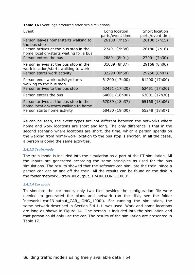
Building traffic models using freely available data | 54
Table 16 Event logs produced after two simulations
Event Long location
parts/event time
Short location
parts/event time
Person leaves home/starts walking to
the bus stop
26100 (7h15) 26100 (7h15)
Person arrives at the bus stop in the home location/starts waiting for a bus
27491 (7h38) 26180 (7h16)
Person enters the bus 28801 (8h01) 27001 (7h30)
Person arrives at the bus stop in the work location/starts walking to work
31039 (8h37) 29168 (8h06)
Person starts work activity 32290 (8h58) 29250 (8h07)
Person ends work activity/starts walking to the bus stop
61200 (17h00) 61200 (17h00)
Person arrives to the bus stop 62451 (17h20) 62451 (17h20)
Person enters the bus 64801 (18h00) 63001 (17h30)
Person arrives at the bus stop in the home location/starts walking to home
67039 (18h37) 65168 (18h06)
Person starts home activity 68430 (19h00) 65248 (18h07)
As can be seen, the event types are not different between the networks where
home and work locations are short and long. The only difference is that in the
second scenario where locations are short, the time, which a person spends on
the walking from home/work location to the bus stop is shorter. In all the cases,
a person is doing the same activities.
5.4.1.3 Train mode
The train mode is included into the simulation as a part of the PT simulation. All
the inputs are generated according the same principles as used for the bus
simulations. The results showed that the software can simulate the train, since a
person can get on and off the train. All the results can be found on the disk in
the folder „network1-train-IN.output_TRAIN_LONG_1000‟.
5.4.1.4 Car mode
To simulate the car mode, only two files besides the configuration file were
needed to generated the plans and network (on the disk, see the folder
„network1-car-IN.output_CAR_LONG_1000‟). For running the simulation, the
same network described in Section 5.4.1.1. was used. Work and home locations
are long as shown in Figure 14. One person is included into the simulation and
that person could only use the car. The results of the simulation are presented in
Table 17.

A case study in Leuven | 55
Table 17 Network #1. Results/car
Event Time
A person ends his home activity 26100 (7h15)
A person enters a car 26100 (7h15)
A person enters link #12 26100 (7h15)
A person leaves link #12 26101 (7h15)
A person enters link #23 26101 (7h15)
A person leaves link #23 28263 (7h51)
A person enters link #34 28263 (7h51)
A person leaves a car 28335 (7h52)
A person starts work activity 28335 (7h52)
A person ends work activity 61200 (17h00)
A person enters a car 61200 (17h00)
A person enters link #43 61201 (17h01)
A person leaves link #43 61274 (17h02)
A person enters link #32 61274 (17h02)
A person leaves link # 32 63436 (17h37)
A person enters link #21 63436 (17h37)
A person leaves link #21 63509 (17h38)
A person enters link #12 63509 (17h38)
A person leaves a car 63581 (17h39)
A person starts home activity 63581 (17h39)
It can be concluded that the agent performs his activities succsesfully using a car
as a transportation mode.
5.4.1.5 Bike mode
As it has been planed, testing a non-car mode is being used on the same
network. The network is the same as for the car and bus. The results (on the
disk, see the folder „network1-bike-IN.output_BIKE_LONG_20‟) of the simulation
are presented in the following Table 18.

Building traffic models using freely available data | 56
Table 18 Network #1. Results/bike
Event Time
A person ends his home activity 26100 (7h15)
A person enters link #12 26100 (7h15)
A person leaves link #12 26100 (7h15)
A person enters link #34 36049 (10h00)
A person leaves link #34 36049 (10h00)
A person starts his work activity 36049 (10h00)
A person ends his work activity 61200 (17h00)
A person enters link #34 61200 (17h00)
A person leaves link #34 61200 (17h00)
A person enters link #12 71149 (19h46)
A person starts his home activity 71149 (19h46)
It can be seen that it is possible to simulate a non-car mode in MATSim. The
person is reaching activity locations by bike, which is proved by the event log
and appropriate time spent on travelling from home to work and from work to
home locations. There is no information regarding the longest links #23 and
#32: the simulation does not show the moment when a person is following these
big links because a person is teleported.
5.4.1.6 U-turns and U-form bus stations
A U-turn (shown in Figure 16) is the maneuver which looks like the letter U (“U-
turn,” 2015). During this maneuver, drivers make a rotation of 180° to change
their direction, for instance if a driver decides to turn back because has to follow
another route due to traffic congestion and for some other reasons.
Figure 16 Example of a U-turn
U-turns are often performed on many roads all over the world. In this thesis, it is
important (since in real traffic drivers make such turns quite often) to
understand if setting up U-turns on the network in MATSim is possible or not in
order to learn the concept and to include it into other traffic models in the future.

A case study in Leuven | 57
Technically, it was not possible to make the curve between two links as it is
shown in Figure 16. The program does not allow to generate U-turns. According
to Rieser (2010), it is not needed because such links may never be part of a
least-cost path. This opinion is supported by the fact that MATSim does not have
the option to generate U-turns. However, it is necessary to find out whether a
person is allowed to turn back in case of an emergency or planned movement. To
check this out, the home location has been placed on link #23 instead of #12 as
in the all other scenarios. For this scenario, the network with short home and
work locations has been used (see Figure 15).
Table 19 shows the results (on the disk see the folder „network1-u-turns-U-
turns_car-car‟), which proved that a person can make a turn in the place where
the nodes are located.
Table 19 Results/U-turns test
Event Time
A person ends his home activity 26100 (7h15)
A person enters link #23 26100 (7h15)
A person enters the car 26100 (7h15)
A person leaves link #23 26101 (7h15)
A person enters link #34 26101 (7h15)
A person leaves link #34 26102 (7h15)
A person starts his work activity 26102 (7h15)
A person ends his work activity 61200 (17h00)
A person enters link #34 61200 (17h00)
A person leaves link #34 61201 (17h00)
A person enters link #43 61201 (17h00)
A person leaves link #43 61203 (17h01)
A person enters link #32 61203 (17h01)
A person leaves link #32 63365 (17h36)
A person enters link #23 63365 (17h36)
A person leaves the car 65526 (18h12)
A person starts his home activity 65526 (18h12)
As can be seen, on the way home, a person does not follow link #21 and #12 to
reach his home location which is located on link #23, but turns on link #23 right
after he passed node #2. Hence, it can be concluded that a person can make a
turn but in the area of nodes, not on the links itself.

Building traffic models using freely available data | 58
In addition, a lot of bus stations have a form similar to U-turns (Figure 17). It is
interesting to know if it is possible to simulate traffic including public transport
departing and arriving at such stations. The scheme of the network shows that
U-turns are generated as a result of making links which start and end at the
same coordinates. In other words, link starts and ends at the same node as it is
shown in Figure 17.
To include this turn into the network, some network modifications have been
made in the network.xml file:
The number of nodes have been limited to two, one for the home location
part and the other for the work location part
In total, four links have been built
Figure 17 Network #1. Bus station in the form of circle
The following Table 20 presents the results after the PT simulation with use of
the U-form stations in the network. The sign „+‟ means that the event mentioned
in the left column is performed.
Table 20 Event logs. Simulation with U-form bus stations included into the network
Events performed by a person Possibility
Leaving/entering location by a person +
Transit walking to/from the bus stop +
Waiting for a bus +
Entering/leaving a bus +
Start/ending an activity +
Events performed by a bus Possibility
Bus departs from a bus stop +
Bus arrives at another bus stop accordingly to the
route
+
Bus waits at the bus stop +
Bus enters/leaves links +
The output shows that the network where the U-turns were constructed did not
have any problems, since buses departures and arrivals at the bus stops
happened according to the schedule. Moreover, there were no problems with a
person‟s plans. The event log file showed that a person is performing his home-
work-home activities without any limitations.

A case study in Leuven | 59
5.4.1.7 Other experiment
In this experiment the coordinates of nodes do not match the link length. For
example, the link length between node #2 and node #3 has been changed from
30000 meters to 30 meters in the network.
As a result (folder „network1-other experiments-do_not‟), a bus entered this link
and left it with the time which suited to the bus speed and distance correctly.
Due to the short link length buses are going through the whole network faster
than in case if the link length was equal to 30000 meters and matched the
coordinates of then nodes where the link is located. Other differences were not
noticed.
5.4.2 Simulating walking
In this scenario (further network #2) the main goal is to find out how an agent
behaves in case walking to work takes less time than taking the bus. The
network consists of four nodes and six links with a link length of 30000 meters
between nodes #2 and #3 (Figure 18). Only one person is included to this
scenario. One bus is running on the links #12, #23, #34, #43, #32 and #21.
Figure 18 Network #2
The results (on the disk see the folder „network2‟) showed that the transit walk
from the home location to the work location is possible and the events are
presented in Table 21.

Building traffic models using freely available data | 60
Table 21 Network #2. Results
Event Time
Person ends his home activity 26100 (7h15)
Person departs from link #12 by walk 26100 (7h15)
Person arrives at his work location 30531 (8h28)
Person starts his work activity 30531 (8h28)
Person ends his work activity 61200 (17h00)
Person departs from link #34 61200 (17h00)
Person arrives on link #12 65631 (18h13)
Person starts his home activity 65631 (18h13)
According to the event log, there is no information regarding the departure and
arrival times on links #23 and #32. This is due to the fact that a person is being
teleported from one location to another, and that walking legs are not mapped
on the road network.
Moreover, the results showed that the bus is going properly and according to the
bus schedule which has been pre-defined in the schedule.xml file. However, the
person ignored the bus and preferred walking directly to the work location.
5.4.3 Switching two buses
The network in this scenario (further network #3) has a straight line, contains six
nodes, eight bus stops and two bus routes which do not interact with each other.
To reach the work location, the person has to switch buses in the middle of the
network between node #3 and node #4 as shown in Figure 19. The first bus
departs at bus stop #1, goes to bus stop #2 and comes back from bus stop #7
to bus stop #8. The second bus departs from bus stop #3 to #4, then goes from
bus stop #5 to #6. The question is if a person can switch buses or not. On this
network, switching buses is possible on links #34 and #43.
Figure 19 Network #3

A case study in Leuven | 61
The results (on the disk see the folder „network3‟) prove that a person can switch
the buses, since to reach the destination, either home or work, a person goes to
the nearest bus stop from where the bus with the needed destination departs.
Table 22 contains the results gathered during the simulation.
Table 22 Network #3. Results
Event Time sec (hours)
Person ends his home activity/starts walking to the
bus stop
26100 (7h15)
Person arrives at bus stop #1 in the home
location/starts waiting for a bus
26100 (7h15)
Person enters bus #1 27901 (7h45)
Person arrives at bus stop #2/starts walking to bus
stop #3
28136 (7h48)
Person arrives at bus stop #3 28292 (7h51)
Person enters bus # 2 30001 (8h20)
Person arrives at bus stop #4/starts walking to the
work location
30294 (8h25)
Person starts his work activity 31545 (8h45)
Person ends his work activity/starts walking to the bus
stop
61200 (17h00)
Person arrives at bus stop #5 62451 (17h21)
Person enters bus #2 63601 (17h40)
Person arrives at bus stop #6/starts walking to bus
stop #7
63836 (17h44)
Person arrives at bus stop #7 63992 (17h46)
Person enters bus #1 65401 (18h10)
Person arrives at bus stop #8 in the home
location/starts walking to home
65694 (18h15)
Person starts his home activity 66945 (18h35)
It can be seen that the results show how a person takes bus #1, reaches the bus
stop in the middle of the network and then walks to another bus stop in order to
take the bus going to the work location. Normally, the event log contains
information regarding the walking distance, between bus stops or the walk from
the location to the bus stop. In this output, the distance of walking for switching
the bus stops on links #34 and #43 have been mentioned as “NaN”, which
means non-available number. MATSim developers explain this by not storing the
route length for all the modes except the car, because of inconsistancies in route
length calculations. Route length is not always updated when MATSim calculates
the optimal decision in every iteration, thus sometimes NaN appears in the
results file.

Building traffic models using freely available data | 62
5.4.4 Simulating multi-modal trips
This scenario (further network #4) has the network (Figure 20) that consists of
two parts, which do not connect with each other. To reach the work location, a
person has to go to the train station by car and then switch mode. Hence, the
main question that should be answered after the simulation is if a person can
switch modes or not. To answer this question, the first part of the network does
not have any PT facilities, but rather is dedicated to the car. To get to the train
station, which is located on links #56 and #65, a person has to reach the train
station by car (on the disk see the folder „network4‟).
Figure 20 Network #4
Results are presented in the following Table 23. As can be seen from the output,
a person is not taking the car, but prefers walking to his work location.
Table 23 Network #4. Results
Event Time
Person ends his home activity 26100 (7h15)
Person walks to the work location 26100 (7h15)
Person arrives at the work location 43417 (12h03)
Person starts work activity 43417 (12h03)
Person ends work activity/person starts walking to
the home location
61200 (17h00)
Person arrives at the home location 78517 (21h48)
Person starts his home activity 78517 (21h48)
The results showed that a person can not switch modes. As it can be seen, a
person is not taking a car as it has been planed in the input data. Instead of this,
a person prefers walking directly to the work location. Thus, the simulation with
car and train transport modes did not succeded, probably due to the fact that a
car should be parked somewhere in the region of station. However, switching two
buses was successful in the network 4 scenario, therefore it can be concluded
that switching modes in MATSim demands more attantion and definetely opens
another question to discuss for further research.

A case study in Leuven | 63
5.4.5 Network with link length zero included
The network in this scenario (further network #5) is a straight line, contains two
persons who are leaving their home at the same time and have a home-work-
home activity. Car mode choice has been chosen for this network. There are six
nodes on the network and the distance between nodes #3 and #4 is equal to 0
meter (Figure 21). The main goal of the simulation is to see how the link with
length 0 meters influences on the whole simulation. The capacity on each link is
defined as three vehicles per hour.
Figure 21 Network #5
The following Table 24 shows the results after the simulation of the network #5
and contains comparison of events happened to both persons and the influence
of the link with 0 meters in length on their behavior. The first two columns
represent the results showed by the initial “intended” plans and the last two
columns represent the results after twenty iterations (on the disk, the files are in
the folder „network5‟).
Table 24 Network #5. Results
Event Iteration 0 Iteration last
Person 1 Person 2 Person 1 Person 2
Person ends
home activity
26100
(7h15)
26100
(7h15)
24529
(6h48)
26100
(7h15)
Person enters
a car
26100
(7h15)
26100
(7h15)
24529
(6h48)
26100
(7h15)
Person enters link #12
27300
(7h35)
26100
(7h15)
24529
(6h48)
26100
(7h15)
Person leaves link #12
27301
(7h35)
26101
(7h15)
24530
(6h48)
26101
(7h15)
Person enters
link #23
27301
(7h35)
26101
(7h15)
24530
(6h48)
26101
(7h15)
Person leaves link #23
27532
(7h38)
26332
(7h19)
24761
(6h52)
26332
(7h19)
Person enters
link #34
27532
(7h38)
26332
(7h19)
24761
(6h52)
26332
(7h19)
Person leaves link #34
27533
(7h38)
26333
(7h19)
24762
(6h52)
26333
(7h19)

Building traffic models using freely available data | 64
Person enters link #45
27533
(7h38)
26333
(7h19)
24762
(6h52)
26333
(7h19)
Person leaves
link #45
27750
(7h42)
26550
(7h22)
24979
(6h56)
26550
(7h22)
Person enters link #56
27750
(7h42)
26550
(7h22)
25051
(6h57)
26550
(7h22)
Person leaves
a car
27822
(7h43)
26622
(7h23)
25051
(6h57)
26622
(7h23)
Work activity starts
27822
(7h43)
26622
(7h23)
25051
(6h57)
26622
(7h23)
Work activity ends
61200
(17h00)
61200
(17h00)
60472
(16h48)
61200
(17h00)
Person enters
a car
61200
(17h00)
61200
(17h00)
60472
(16h48)
61200
(17h00)
Person enters link #56
61200
(17h00)
61200
(17h00)
60472
(16h48)
61672
(17h07)
Person leaves
link 56
62401
(17h20)
61201
(17h00)
60473
(16h48)
61673
(17h07)
Person enters link #65
62401
(17h20)
61201
(17h00)
60473
(16h48)
61673
(17h07)
Person leaves link #65
62474
(17h21)
61274
(17h01)
60546
(16h49)
61746
(17h09)
Person enters
link #54
62474
(17h21)
61274
(17h01)
60546
(16h49)
61746
(17h09)
Person leaves link #54
62691
(17h25)
61491
(17h04)
60763
(16h52)
61963
(17h11)
Person enters
link #43
62691
(17h25)
61491
(17h04)
60763
(16h52)
61963
(17h11)
Person leaves link #43
62691
(17h25)
61492
(17h04)
60764
(16h52)
61964
(17h12)
Person enters link #32
62692
(17h25)
61492
(17h04)
60774
(16h53)
61964
(17h12)
Person leaves
link #32
62923
(17h28)
61723
(17h08)
60995
(16h56)
62195
(17h16)
Person enters link #21
62923
(17h28)
61723
(17h08)
60995
(16h56)
62195
(17h16)
Person leaves
link #21
62996
(17h30)
61796
(17h09)
60995
(16h56)
62268
(17h18)
Person enters link #12
62996
(17h30)
61868
(17h11)
61068
(16h58)
62268
(17h18)
Person leaves a car/starts the
home activity
63068
(17h31)
61868
(17h11)
61140
(16h59)
62340
(17h19)

A case study in Leuven | 65
As can be seen, the link with a length of 0 meters influences the simulation
results significantly. In the initial iteration #0, the results showed that both
persons leave their home at the same time. While person #2 is going through all
the links alone, reaches his work location and starts his work activity, only after
this moment person #1 starts entering link #12 in his car. The same situation
happens on the way back. Both agents leave their work locations at the same
time, but only person #2 is going on the entire network and reaches his home
location alone. Meanwhile, person #1 is waiting in his car at the work location
and starts moving only after (according to the results around 8 minutes) person
#2 has started his home activity.
In marked contrast, after 20 iterations the results showed that during the
simulation it was taken into account the early departure from the home location
for one of the persons. Instead of 7h15 person 1 leaves his home at 6h48, starts
his work activity earlier and before person 2 leaves his home.
In addition, despite the fact that link #12 has enough capacity, a person is not
able to enter link #12 before another person has started his work activity.
However, during the testing of the same network but without the link of a length
equals to zero, it was mentioned that both persons enter link #12 at the same
time and only one of them starts waiting to enter rest of the network while
another one is getting to his work location (on the disk, see the results in the
folder „network5-comment‟).
To conclude, the link with length zero is an unwanted link for the network. First
of all, such a link is not long enough to hold a vehicle, and second, the capacity
of the link before cannot be too large, since it makes all the vehicles arrive at the
link with length zero at the same time. Hence, such a link makes playing with
large link capacity problematic.
5.4.6 Network with the low capacity link included
This scenario (further network #6) has the network that consists of four nodes
with home-work-home activity. Two persons are included into the simulation.
The link between the home and work location parts has a low capacity (no more
than one car per hour). Four transport modes - car, bus, train and bike have
been included in the scenario.
Figure 22 Network #6

Building traffic models using freely available data | 66
Car mode
The simulation includes the network (Figure 14) with two persons. The car is the
transport mode. The results are presented in Table 25 (on the disk, see the
folder „network6-car-network6_car‟).
Table 25 Network #6. Results/car
Event Person 1 Person 2
Person ends his home
activity
26100 (7h15) 26100 (7h15)
Person enters a car 26100 (7h15) 26100 (7h15)
Person enters link #12 26104 (7h15) 26100 (7h15)
Person leaves link #12 26105 (7h15) 26101 (7h15)
Person enters link #23 26105 (7h15) 26101 (7h15)
Person leaves link #23 31863 (8h51) 28263 (7h51)
Person enters link #34 31863 (8h51) 28263 (7h51)
Person leaves a car 31935 (8h52) 28335 (7h52)
Person starts work activity 31935 (8h52) 28335 (7h52)
Person ends work activity 61200 (17h00) 61200 (17h00)
Person enters a car 61200 (17h00) 61200 (17h00)
Person enters link #43 61201 (17h00) 61201 (17h00)
Person leaves link #43 61276 (17h01) 61274 (17h01)
Person enters link #32 61276 (17h01) 61274 (17h01)
Person leaves link #32 67036 (18h37) 63436 (17h37)
Person enters link #21 67036 (18h37) 63436 (17h37)
Person leaves link #21 67109 (18h38) 63509 (17h38)
Person enters link #12 67109 (18h38) 63509 (17h38)
Person leaves link #12 67181 (18h39) 63581 (17h40)
Person leaves a car 67181 (18h39) 63581 (17h40)
Person starts his home
activity
67181 (18h39) 63581 (17h40)
The results showed that persons ended their home activity and entered their cars
at the same time. However, person 2 entered link #12 earlier, since the link #23
can accommodate only 1 vehicle. Thus, person #1 had to wait till a person #2
has started his work activity, since the link capacity was reached. Besides, after
20 iterations the simulation has taken into account the fact of early departure of
person 1. The results performed after 20 ietrations can be found on the disk.
Bike mode
In this simulation, two persons are included and bikes have been chosen as a
mode choice. The following Table 26 shows the results. All the codes and the
output results are included in the folder „network6-bike-network6bike‟ on the
disk.

A case study in Leuven | 67
Table 26 Network #6. Results/bike
Event Person 1 Person 2
Person ends his home activity 26100 (7h15) 26100 (7h15)
Person departs by bike/link #12 26100 (7h15) 26100 (7h15)
Person enters link #34 27504 (7h38) 27504 (7h38)
Person leaves link #34 27504 (7h38) 27504 (7h38)
Person starts his work activity 27504 (7h38) 27504 (7h38)
Person ends work activity 61200 (17h00) 61200 (17h00)
Person enters link #34 61200 (17h00) 61200 (17h00)
Person leaves link #34 61200 (17h00) 61200 (17h00)
Person enters link #12 62604 (17h23) 62604 (17h23)
Person starts his home activity 62604 (17h23) 62604 (17h23)
It can be seen that despite the fact that link # 23 and # 32 have the capacity of
one vehicle, both persons are going through all the links together and without
delays. Therefore, it can be concluded that if a person is using a bike as a mode
choice, a person is not following the rules of the simulation, and as it has been
mentioned in chapter 5.2.2, MATSim is transferring a person from home to work
locations. In addition, in the output there is no information about the longest
part of the road-link #23, #32, since MATSim does not show that a person is
going on these long links on a bike.
Bus mode
The next network includes the simulation of PT. Three persons start their home
activity at the same time. At every bus stop only two buses with a capacity of
two passengers depart. One of them departs before arriving of persons at the
bus stop, so only two buses are available for three persons (one bus has a
capacity of two people). The main idea of the simulation is to see what happens
if the bus is full and there is no extra bus which can accommodate the rest of the
passengers. The following Table 27 represents the results (on the disk see
network6-network6bus_3pers1veh).
Table 27 Network #6. Results/bus
Event Person 1 Person 2 Person 3
Person ends his home
activity
26100 (7h15) 26100 (7h15) 26100 (7h15)
Person arrives at bus
stop #1 by walk
27491 (7h38) 27491 (7h38) 27491 (7h38)
Person enters a bus - 28202 (7h50) 28201 (7h50) Person leaves a bus at
bus stop #2
- 30441 (8h27) 30440 (8h27)
Person arrives at work
location and starts work activity
- 31692 (8h48) 31691 (8h48)
Person ends work
activity
- 61200 (17h00) 61200 (17h00)
Person arrives at bus
stop #3 by walk
- 62451 (17h20) 62451 (17h20)

Building traffic models using freely available data | 68
Person enters the bus - 63002 (17h30) 63001 (17h30)
Person arrives at bus stop #4
- 65241 (18h07) 65240 (18h07)
Person leaves the bus/
starts walking to home location
65241 (18h07) 65240 (18h07)
Person starts his home activity
- 66632 (18h30) 66631 (18h30)
The results showed that all three persons ended their home activity at the same
time and arrived at the bus stop at the same time. Therefore, only two of them
(#2 and #3) could get on the bus in time and completed their plans successfully.
Person #1 could not get on the bus, since there was no extra bus for him. The
output results showed that this person was stuck at the bus stop. It can be
concluded, that a person cannot be transferred to activity location if there are no
vehicles included into the simulation of PT, moreover, according to this output a
person does not prefer walking to his work location, but prefers to stay at the
bus stop.
Train mode
In this network, the train mode is used. There are three persons who leave their
home at the same time. There are three trains with a capacity of one person per
train. All trains depart with an interval of ten minutes.
The results (see the folder „network6-train-train_6‟) showed that if all the
vehicles are full of passengers, the rest of the persons are allowed to get on the
next train which departs a few minutes later. The starting time of the work
activity directly depends on the time of persons arriving at the station, according
to the arrival time of the train.
Afterwards, all six networks have been tested, as it was pointed out in Section 2,
large Leuven scenario can be simulated according to the skills gathered during
simulating the small networks.
5.5 Leuven scenario
The Leuven scenario in this thesis is the small model of the real Leuven network.
This small scenario is the network, which has four areas located outside the city
(on the network these are the A, B, C and D locations) and the city center with
nine „cells‟ inside. On each link in the city center, there are one home and one
work location. On each loop in the outskirts there is also one work and one home
location. Ten people live in each home location in the city center. On each home
location in the outskirts, 25 people are accomodated.
Everybody has the schedule home-work-home activity except those agents
visiting the hospital. These agents have the schedule home-work-home-visit-
home activity. People who work in the hospital do not have the visit activity.

A case study in Leuven | 69
To simulate this Leuven scenario it is necessary to define which input files
needed to be included. First of all, the network.xml should be created according
to the scheme of Leuven shown in Figure 23.
Figure 23 Leuven city center with suburbs
Furthermore, the plans.xml file should be generated using the
MatsimStubDataGenerator (on the disk, see the folder
„MatsimStubDataGenerator‟). This generator has been created by the
transportation behavior research group of IMOB (the Transportation Research
Institute, Hasselt University) specifically for this scenario. It helps generating
plans.xml with a large amount of agents and avoids typing the code manually.
The data generator demands five csv files to fill in:
Home locations
Work locations
Home distribution

Building traffic models using freely available data | 70
Work distribution
Schedules
The Home_locations.csv file contains three columns: type, latitude and longitude.
As for the type, it has been mentioned there are two types of area defined as a
home location: the suburbs and the city center. Suburbs are located in the A, B,
C and D areas, while the city center has 24 links inside. Latitude and longitude
are the x and y axes where locations are situated.
In the Work_locations.csv file, besides the type of columns mentioned above,
there are four additional columns describing the earliest_start_time,
latest_start_time, earliest_start_time and latest_end_time of the work activity.
According to the data gathered and described in Section 4, the time interval to
start a work activity ranges between 08:30:00 and 09:30:00. For the end time of
the work activity this interval is between 17:30:00 and 18:00:00. Moreover,
those people who work at the hospital (calculations can be found in the following
text) have been divided into four categories.
Shift workers who start working at 06:00:00
Shift workers who start working at 14:00:00
Shift workers who start working at 22:00:00
Regular office hours workers who start working at 08:30:00
Regarding the Home_distribution.csv file, the percentage of people living in the
suburbs and the city center should be calculated. In case of the Leuven scenario
in this research, in total 340 people were included into the simulation. As
mentioned above, 25 people live in every suburb area (25*4=100), and 240
people live on every link in the city center (10*24=240). This means that ten
people live on one of the 24 links. Hence, in percentages of amount of people
living in the suburbs area is equal to 29% and those living in the city center
equals to 71%.
Another file that needs to be filled in in order to generate the plans.xml is the
Work_distribution.csv file. There are two types of work: hospital (that means
amount of people working in the hospital) and normal (that means the amount of
people who work in any other random location except hospital). To spread the
total number of living people per type, the data obtained in Section 4 has been
used. Hospital type includes percentage of doctors and staff who are working
regular office hours. Normal type includes nurses and other employees who work
in shifts. Hence, 81% of people work in random locations and 19% work in the
hospital.
The Schedules.csv file contains categories (people who work in random locations
and people who work in the hospital). One category of hospital workers and one
category of workers working in random locations have the schedule home-work-
home. One category of those who work in random locations have the schedule
home-work-home-visit-home activity.

A case study in Leuven | 71
To run the MatsimStubDataGenerator it is necessary to run the following
command:
java -cp MatsimStubDataGenerator.jar MatsimStubDataGenerator 340
1800 3600 "18:00:00" "20:00:00"
Where:
340-total number of people included into the simulation
1800 sec-minimal required default time to get from origin to destination
3600 sec-minimum duration of a hospital visit
18:00:00-start of visiting hours
20:00:00-end of visiting hours
To get the output it is necessary to run the following:
path\output.txt
Afterwards it is possible to save data from txt to the XML format file.
As for the configuration parameters, one more activity type, „visit‟, has been
included. Typical duration is set up as one hour, since the literature review
showed that this time is enough for people to make a hospital visit. Moreover,
the same duration was set up in the MatsimStubDataGenerator, in order to
include this time to the plans.xml. In addition, for PT parameters, transit module
includes „pt‟ parameter name.
In the network, as it has been shown in Figure 24, different modes of transport
have been used. There is a train station and a bus stop at every link. Colored
lines are the bus lines (BL). For clear observation, the scheme of the city center
is shown in Figure 24.

Building traffic models using freely available data | 72
Figure 24 Leuven city center
The simulation of the network was successful and resulted in 16422 events
included in the event log, which can be found in the folder „Leuven‟ on the disk.
Since the plans.xml file contains only car as a mode choice, due to generation of
schedule.xml it was achieved implementation of PT into the network and
possibility to allow agents using buses and trains to reach their destinations in
later iterations. The results showed that in the first iterations agents only used
their cars. Meanwhile, all the PT modes departure and arrived at the locations
according to the schedules.xml file. Vehicles‟ id‟s are the same as the id‟s of
agents. In the later iterations it was noticed that all the agents who were
supposed to take PT did not do that. Instead of the use of PT agents preferred to
walk to their destinations and even avoided car use. Moreover, they did not walk
to bus stops or train stations. This observation is similar to the results gathered
in the network simulated in Section 5.4.4, where agents were not able to
perform multi-modal trips. In addition, according to the results, the work activity
of some agents is located in the region of link #3141 and agents start working
over there in different shifts and in office hours. Those agents working in random

A case study in Leuven | 73
locations start their work activities at different parts of the network. Some
agents work in the hospitals during different shifts as planned.
For some more tests, congestion effects on the network have been analyzed (see
the folder „Leuven-congestion‟ on the disk). For the entire network, an average
capacity of 1000 vehicles per link per hour was specified. In order to provoke
and see the effect of congestion, links #4131, #3141, #4142 and #4241 were
closed by means of reducing the capacity to 0 vehicles per hour. These links
have been chosen, since they were closest to the hospital where 19% of the
agents had a fixed working location. The following results were found:
Closed links do not influence on finishing the home activity of those agents
living in the home locations accomodated in the region of these links
Agents living in the region of closed links cannot do any activities right
after they finish their home activities
Agents whose work location is in the region of closed links are stuck on
these links
Agents whose work location is in the region of closed links cannot start
their work activity
Buses cannot follow these closed links and are being stuck
To sum up, performing activities by agents is significantly decreased by those
parts of the network where capacity reduced. Moreover, based on the practice
gathered during early simulations it can be safely assumed that this problem
does not spread over to non-car modes and trains since those are teleported by
the software.

Building traffic models using freely available data | 74
A case study in Leuven | 75
CONCLUSION
This thesis explores the possibilities to develop a traffic model, based on freely
available data. Data provided by the University Hospitals of Leuven partially
contributed to the Leuven scenario in this thesis and in future research to the
SMART-PT project, which goal is to create a self-adaptive public transportation
system.
The first part of the research consisted of the literature study, which enabled to
get insight in the nature of traffic models, their structure, their benefits and their
drawbacks. Therefore, the hospital-related data was collected for further traffic
modelling. The main focus in this part of the thesis was to identify the
distribution of hospital visitors throughout the day. To begin with, the search was
started with personnel arrivals and departures per category: staff working during
regular office hours (doctors and 90% of administrative personnel) and those
working in shifts (nurses and 10% of administrative personnel). As for
commuting type chosen by personnel, according to the annual report, the
biggest percentage of employees is commuting by car (57%). Fifteen percent
preferred to travel as a car passenger, while the remaining 28% was divided
equally between the use of public transportation and walking and cycling.
Working hours found on the hospital website allowed to determine the time of
employees‟ arrivals and departures. The total number of hospitalizations allowed
to calculate the number of single-day-hospitalizations and consultations in the
year 2013, found in the annual report. The average amount of patients arriving
and leaving the hospital during one day has been calculated. Regarding those
coming to visit patients, the literature study showed the average number of trips
per hospital bed in one day, what allowed to calculate the number of daily visits.
According to visiting hours, mentioned on the hospital webpage, calculated visit
trips were distributed throughout the day. To sum up, gathering freely available
data was quite hard due to limited sources. The administration of the hospitals
does not cooperate with students and can only provide annual reports with
limited information. The annual report should be extended in its information
concerning some daily numbers, as calculated in Table 15.
During the second part, the simulations were performed using MATSim. Different
scenarios, modes of transport and networks‟ characteristics were tested.
In total, six networks were tested and it can be cocnluded that all the simulations
succeeded. As for the first network, the results did show that a person was able
to do his activities according to the schedule intended in the plans.xml. During
the simulation, different transport modes could be used:
Car
Train
Bus

Building traffic models using freely available data | 76
Bike
When a person is using the car, train or bus, the event log shows the entire
route a person traveled through the network from his origin to his destination. In
marked contrast, when a person is going with non-car mode, such as bike, or
with non-road based mode, such as the train, the output results show
independence of a mode from the network, since a person is being teleported
(the same situation occurred in network #2 where walking was analyzed). When
a person has to reach the bus stop to take a bus further, a person is making a
walking transit as the results show. In addition, testing of u-turns showed that a
vehicle can only make a turn in the region of the nearest node, but not on the
link itself. The efficiency of this option in MATSim can be determined and
explained in future research.
According to the network, the distance between the home location and bus stops
is around 20% shorter than the distance walked by a person during his transit.
In one of the networks the walking transit distance was shown as “NaN”, which
means non-available number. Due to the reason explained in Section 5.4.3., the
software creators recommend to develop the model for calculating route length
for every specific scenario, what defenetily can become a future research idea.
Network #3 demostrated that switching buses is allowed in MATSim. It was
found that a person is able to make a walking transfer to a bus station, then pick
up a bus and then switching to another bus on the same link. However, in
network #4, switching different modes was not possible. Due to the fact that a
car should be parked in the area of train station makes switching car-train modes
impossible. Moreover, car mode was replaced by another train and the simulation
did not succeed despite the fact that both modes were public transport. As a
result, a person just preffered walking to his work location. According to the
results gathered in this thesis, it can be concluded that a possibility of network
connectivity in case of lanes laying on different levels is under discussion.
In network #5 and #6, the effect of links with length equal to 0 and low capacity
link have been tested. It was found that the link with 0 meters in length
encourages a person to wait at his home location till the moment another person
has started his work activity. The effect of low capacity links resulted in forcing
one vehicle to wait while another vehicle has reached its destination as well as
the link with length 0 meters. This can influence the early departure time of
agents.
After all testing scenarios, the Leuven scenario was simulated. To run it the
following set of files was required:
Config.xml
Network.xml
Plans.xml
Schedules.xml

A case study in Leuven | 77
Vehicles.xml
Plans.xml has been created by means of the MatsimStubDataGenerator. Results
showed 16422 events. However, multi-modal trips did not occur.
Initially, it was assumed that agents were not allowed to use PT, because they
had a car available for all the activities in their schedule. After the simulation, it
was identified that this was not the reason, since the trial to switch car mode to
pt mode in the plans of some agents did not succeed and just forved agents to
make a transit walk. In the first iterations agents took their cars while in the last
iterations, they just preferred walking to their destinations. Such an effect is
similar to the one revealed during the simulation of multi-modal trips in Section
5.4.4.
In addition, congestion effects have been analyzed. The results showed that
closed links influenced the entire simulation significantly. Those agents working
and leaving in the region of closed links could not perform any activities and just
made „stuck‟ activity, that means no movements.

Building traffic models using freely available data | 78
A case study in Leuven | 79
DISCUSSION
The city of interest is Leuven and only a small region containing the center of the
city has been taken into account for the research. This limitation has a practical
reason: micro-simulation requires a lot of computer resources and detailed
simulations are only feasible when the number of individuals is limited.
In this study, only one day (Tuesday or Thursday) of August is used for the
simulation, so the effect of the students, that is assumed to generate the main
part of the city‟s vulnerable road users (e.g. pedestrians or cyclists), can be
safely ignored.
Some parts of the city were not modeled in detail: the „Interbrew‟ site, the large
offices named „Boerenbond‟ in the center and the new office buildings along the
railway at the opposite side of the train station. For this study they were
assumed to not influence bus operations. However, it can be said that to
determine the impact of those locations on the traffic flow would be an
interesting field for future research.
One of the problems during the simulations of the Leuven network was
considered to be the identification of the effects of multi-modal daily tours of
hospital visitors. In reality, their influence on the bus network is rather unknown,
since they could choose different modes of transport for the different parts of
their journey. For example, one can decide to take the bus to go to work, but
walk to a restaurant during the lunch break. In this case, it was important to
identify if multi-modal tours are handled in MATSim and to estimate the effect on
the demand for bus trips. The fact of impossibility to make multi-modal trips
have been proved in this thesis during the simulating small Leuven scenario in
this research.
Particularly, it was planned that the third part in this research, the comparison of
bus-line profiles, would play a role of the model estimator. However, generating
and comparison these bus-line profiles seemed to be meaningless, since multi-
model trip could not be included in the simulation.
In conclusion, it can be said that this research topic, „Building traffic models
using freely available data‟, has been approached from different sides. Types of
traffic models became familiar based on the knowledge gathered during the
literature study. Bulding and simulating small, but different scenarios have been
done. All the results have been analyzed and discussed. The Leuven network
itself has also been modelled, using the hospital-related data gathered during the
first part of the research. All the results have been analyzed and discussed.

Building traffic models using freely available data | 80

A case study in Leuven | 81
REFERENCES
Agent-Based Transport Simulations | MATSim. (2014). Retrieved November 18,
2014, from http://www.matsim.org/
Ahmed, B. (2012). The Traditional Four Steps Transportation Modeling Using
Simplified Transport Network: A Case Study of Dhaka City, Bangladesh.
International Journal of Advanced Scientific Engineering and Technological
Research, 1(1), 19–40.
ALBATROSS - Travel Forecasting Resource. (n.d.). Retrieved January 4, 2015,
from http://tfresource.org/ALBATROSS
Arentze, T., Hofman, F., van Mourik, H., & Timmermans, H. (2000). ALBATROSS:
Multiagent, Rule-Based Model of Activity Pattern Decisions. Transportation
Research Record, 1706(1), 136–144. http://doi.org/10.3141/1706-16
Arsalan Effendi. (2014). Making MATSim operational for flemish region
(Internship). Belgium, Hasselt: Instituut voor Mobiliteit (IMOB).
B. Haut, G. Bastin, & Y. Chitour. (2005). A MACROSCOPIC TRAFFIC MODEL FOR
ROAD NETWORKS WITH A REPRESENTATION OF THE CAPACITY DROP
PHENOMENON AT THE JUNCTIONS. Universite Catholique de Louvain,
Batiment Euler, 6.
Bruno Kochan, Tom Bellemans, Davy Janssens, & Geert Wets. (2008). Assessing
the impact of fuel cost on traffic demand in Flanders using (p. 7).
Presented at the Travel Demand Management, Vienna: Transportation
Research Institute, Hasselt University.
Buehler, R. (2008). Transport Policies, Travel Behavior, and Sustainability: A
Comparison of Germany and the U.S. ProQuest.
Davy Janssens. (2014a). Management and prediction of travel demand. Hasselt
University.
Building traffic models using freely available data | 82
Davy Janssens. (2014b). Prediction of travel demand and data inputs. Lecture,
Hasselt.
Davy Janssens. (n.d.). Activity based models: course introduction.
Delphi method. (2015, July 25). In Wikipedia, the free encyclopedia. Retrieved
from
https://en.wikipedia.org/w/index.php?title=Delphi_method&oldid=672953
403
Emergency medicine | UZ Leuven. (2014). Retrieved December 25, 2014, from
http://www.uzleuven.be/en/emergencies
Guy Mannaerts. (2013). UZ_Leuven_jaarverslag_2013_innovatie. Leuven.
Health Sciences campus Gasthuisberg | UZ Leuven. (n.d.). Retrieved November
26, 2014, from http://www.uzleuven.be/uz-leuven-bouwt-voor-u/health-
sciences-campus
Hospitalization | Define Hospitalization at Dictionary.com. (n.d.). Retrieved
January 10, 2015, from
http://dictionary.reference.com/browse/hospitalization
IMOB. (2014). “ERA-NET Transport III: Domain 2 Traveller of the Future –
SMART – PT” SMART – PT : Smart Adaptive Public Transport. Buur –
bureau van urbanisme cvba Leuven: Instituut voor Mobiliteit (IMOB).
iRail.be. (n.d.). Retrieved July 28, 2015, from https://irail.be
Jan Paesen. (2011). KU Leuven staff commute survey 2011 – KU Leuven.
Retrieved November 29, 2014, from
http://www.kuleuven.be/transportation/commute-survey-2011
Joe Castiglione, Mark Bradley, & John Gliebe. (2014). Activity-based Travel
Demand Models: A primer (No. 031031-4034) (p. 170). White River
Junction, VT: The National Academies.

A case study in Leuven | 83
Juan de Dios Ortuzar, & Luis G. Willumsen. (2011). Modelling transport (4th ed.).
United Kingdom: John Wiley & Sons, Ltd.
Leuven. (2016, January 3). In Wikipedia, the free encyclopedia. Retrieved from
https://en.wikipedia.org/w/index.php?title=Leuven&oldid=697960533
Lieve Creemers. (2014, February). orderinf.eu » presentations third seminar
available. Retrieved from http://orderinf.eu/?p=886&lang=en
Luk Knapen, & Jan Vuurstaek. (2014, November). Master‟s thesis appointment.
Marcel Rieser. (2010). MATSim-T: Architektur und Rechenzeiten. Berlin: ETH,
Eidgenössische Technische Hochschule Zürich, Institut für
Verkehrsplanung und Transportsysteme.
Marvin R. Duncan, & Earl O. Heady. (1976). A programming model for analysis of
nonmetropolitan hospital services systems and application of the model
(No. 50011). Iowa: Iowa State University.
MATSim User‟s guide. (2013). Retrieved from matsim.org/docs/userguide
OpenStreetMap. (2014). Retrieved October 29, 2014, from
http://www.openstreetmap.org/#map=5/51.500/-0.100
OpenStreetMap Wiki. (2014). Retrieved October 29, 2014, from
http://wiki.openstreetmap.org/wiki/Main_Page
Over UZ Leuven | UZ Leuven. (2014). Retrieved November 26, 2014, from
http://www.uzleuven.be/over-ons
Overzicht artsen en specialisten | UZ Leuven. (n.d.). Retrieved January 10, 2015,
from http://www.uzleuven.be/artsen
project_details. (n.d.). Retrieved January 13, 2015, from
https://www.uhasselt.be/UH/research/Research-structures/Research-
groups-per-discipline-group/en-projecten_DOC/en-
project_details.html?pid=8803&t=en

Building traffic models using freely available data | 84
Rolf Moeckel, & Klaus Spiekerman. (2003). Creating a Synthetic Population.
Presented at the 8th Internation Conference on Computers in Urban
Planning and Urban Management (CUPUM), Sendai, Japan.
Rye Baerg. (2014, May). Improving modeling and data collection for active
transportation. Presented at the Safe Routes to School National
Partnership, Southern California.
Scott Miller. (2011). Traffic modeling (p. 13).
Serge Hoogendoorn, & Victor Knoop. (2004). The transport system and transport
policy. In Traffic flow theory and modelling (p. 35).
Station Leuven - Google Maps. (n.d.). Retrieved January 13, 2015, from
https://www.google.be/maps/place/Station+Leuven/@50.8785794,4.6931
622,15z/data=!4m2!3m1!1s0x47c1672cad4fc3e7:0x7986b49e27588b77?
hl=en
Theo Arentze, & Harry J.P. Timmermans. (n.d.). ALBATROSS-A Learning-based
transportation oriented system (p. 23). 5600 MB, Eindhoven, The
Netherlands: Eindhoven University of Technology.
Theo Arentze, Harry Timmermans, Frank Hofman, & Nelly Kalfs. (1998). Data
needs, data collection, and data quality requirements of activity-based
transport demand models. The Netherlands, Eindhoven: Eindhoven
University of Technology.
Tom Bellemans, Davy Janssens, Geert Wets, Theo Arentze, & Harry
Timmermans. (2010). Implementation framework and development
trajectory of the FEATHERS Activity-Based Simulation platforf. Presented
at the TRB 2010 Annual Meeting.
Traffic simulation. (2014, November 22). In Wikipedia, the free encyclopedia.
Retrieved from

A case study in Leuven | 85
http://en.wikipedia.org/w/index.php?title=Traffic_simulation&oldid=63493
8041
UHasselt. (2014). Behaviourally-sensitive simulator design ready for the
calculation of Mobility-EV scenarios.
U-turn. (2015, August 1). In Wikipedia, the free encyclopedia. Retrieved from
https://en.wikipedia.org/w/index.php?title=U-turn&oldid=674113275
UZ Leuven - Universitair ziekenhuis. (2014). Retrieved November 27, 2014, from
http://www.uzleuven.be/en
Vind een specialist via discipline | UZ Leuven. (2014). Retrieved December 25,
2014, from http://www.uzleuven.be/specialisaties
Vlaamse statistieken. (2014). Retrieved October 29, 2014, from
http://www.ond.vlaanderen.be/onderwijsstatistieken/
Wang, W., & Wets, G. (2012). Computational Intelligence for Traffic and Mobility.
Springer Science & Business Media.
Welton, J. M. (2011). Hospital nursing workforce costs, wages, occupational mix,
and resource utilization. The Journal of Nursing Administration, 41(7-8),
309–314. http://doi.org/10.1097/NNA.0b013e3182250a2b
XML. (2015, July 23). In Wikipedia, the free encyclopedia. Retrieved from
https://en.wikipedia.org/w/index.php?title=XML&oldid=672770310
Zmud, J., Lee-Gosselin, M., Carrasco, J. A., & Munizaga, M. A. (2013). Transport
Survey Methods: Best Practice for Decision Making. Emerald Group
Publishing.

Building traffic models using freely available data | 86

Auteursrechtelijke overeenkomst
Ik/wij verlenen het wereldwijde auteursrecht voor de ingediende eindverhandeling:
Building traffic models using freely available data
Richting: Master of Transportation Sciences-Mobility Management
Jaar: 2016
in alle mogelijke mediaformaten, - bestaande en in de toekomst te ontwikkelen - , aan de
Universiteit Hasselt.
Niet tegenstaand deze toekenning van het auteursrecht aan de Universiteit Hasselt
behoud ik als auteur het recht om de eindverhandeling, - in zijn geheel of gedeeltelijk -,
vrij te reproduceren, (her)publiceren of distribueren zonder de toelating te moeten
verkrijgen van de Universiteit Hasselt.
Ik bevestig dat de eindverhandeling mijn origineel werk is, en dat ik het recht heb om de
rechten te verlenen die in deze overeenkomst worden beschreven. Ik verklaar tevens dat
de eindverhandeling, naar mijn weten, het auteursrecht van anderen niet overtreedt.
Ik verklaar tevens dat ik voor het materiaal in de eindverhandeling dat beschermd wordt
door het auteursrecht, de nodige toelatingen heb verkregen zodat ik deze ook aan de
Universiteit Hasselt kan overdragen en dat dit duidelijk in de tekst en inhoud van de
eindverhandeling werd genotificeerd.
Universiteit Hasselt zal mij als auteur(s) van de eindverhandeling identificeren en zal geen
wijzigingen aanbrengen aan de eindverhandeling, uitgezonderd deze toegelaten door deze
overeenkomst.
Voor akkoord,
Naumova, Iuliia
Datum: 11/01/2016