Preface - · PDF fileFor more detail, we recommend Section 1, ... the letter N with or...
88
Preface Stochastic control theory is a relatively young branch of mathematics. The beginning of its intensive development falls in the late 1950s and early 1960s. ~urin~ that period an extensive literature appeared on optimal stochastic control using the quadratic performance criterion (see references in Wonham [76]). At the same time, Girsanov [25] and Howard [26] made the first steps in constructing a general theory, based on Bellman's technique of dynamic programming, developed by him somewhat earlier [4]. Two types of engineering problems engendered two different parts of stochastic control theory. Problems of the first type are associated with multistep decision making in discrete time, and are treated in the theory of discrete stochastic dynamic programming. For more on this theory, we note in addition to the work of Howard and Bellman, mentioned above, the books by Derman [8], Mine and Osaki [55], and Dynkin and Yushkevich [12]. Another class of engineering problems which encouraged the development of the theory of stochastic control involves time continuous control of a dynamic system in the presence of random noise. The case where the system is described by a differential equation and the noise is modeled as a time continuous random process is the core of the optimal control theory of diffusion processes. This book deals with this latter theory. The mathematical theory of the evolution of a system usually begins with a differential equation of the form at = f(t,xt) with respect to the vector of parameters x of such a system. If the function f (t,x) can be measured or completely defined, no stochastic theory is needed. However, it is needed if f(t,x) varies randomly in time or if the errors of measuring this vector cannot be neglected. In this case f(t,x) is, as a rule,
Transcript of Preface - · PDF fileFor more detail, we recommend Section 1, ... the letter N with or...

Preface
Stochastic control theory is a relatively young branch of mathematics. The beginning of its intensive development falls in the late 1950s and early 1960s. ~ u r i n ~ that period an extensive literature appeared on optimal stochastic control using the quadratic performance criterion (see references in Wonham [76]). At the same time, Girsanov [25] and Howard [26] made the first steps in constructing a general theory, based on Bellman's technique of dynamic programming, developed by him somewhat earlier [4].
Two types of engineering problems engendered two different parts of stochastic control theory. Problems of the first type are associated with multistep decision making in discrete time, and are treated in the theory of discrete stochastic dynamic programming. For more on this theory, we note in addition to the work of Howard and Bellman, mentioned above, the books by Derman [8], Mine and Osaki [55], and Dynkin and Yushkevich [12].
Another class of engineering problems which encouraged the development of the theory of stochastic control involves time continuous control of a dynamic system in the presence of random noise. The case where the system is described by a differential equation and the noise is modeled as a time continuous random process is the core of the optimal control theory of diffusion processes. This book deals with this latter theory.
The mathematical theory of the evolution of a system usually begins with a differential equation of the form
at = f(t,xt)
with respect to the vector of parameters x of such a system. If the function f (t,x) can be measured or completely defined, no stochastic theory is needed. However, it is needed if f(t,x) varies randomly in time or if the errors of measuring this vector cannot be neglected. In this case f(t,x) is, as a rule,

representable as b(t,x) + a(t,x)[, where b is a vector, cr is a matrix, and 5 , is a random vector process. Then
It is convenient to write the equation in the integral form
where xo is the vector of the initial state of the system. We explain why Eq. (2) is preferable to Eq. (1). Usually, one tries to choose the vector of parameters x, of the system in such a way that the knowledge of them at time t enables one to predict the probabilistic behavior of the system after time t with the same certainty (or uncertainty) to the same extent as would knowledge of the entire prior trajectory xs (s 5 t). Such a choice of parameters is con- venient because the vector x, contains all the essential information about the system. It turns out that if x, has this property, it can be proved under rather general conditions that the process 5 , in (2) can be taken to be a Brownian motion process or, in other words, a Wiener process w,. The derivative of 5, is then the so-called "white noise," but, strictly speaking, 5, unfortunately cannot be defined and, in addition, Eq. (1) has no immediate meaning. How- ever, Eq. (2) does make sense, if the second integral in (2) is defined as an Ito stochastic integral.
It is common to say that the process x, satisfying Eq. (2) is a diffusion process. If, in addition, the coefficients b, o of Eq. (2) depend also on some control parameters, we have a "controlled diffusion process."
The main subject matter of the book having been outlined, we now indicate how some parts of optimal control theory are related to the contents of the book.
Formally, the theory of deterministic control systems can be viewed as a special case of the theory of stochastic control. However, it has its own unique characteristics, different from those of stochastic control, and is not considered here. We mention only a few books in the enormous literature on the theory of deterministic control systems: Pontryagin, Boltyansky, Gamkrelidze, and Mishchenko [60] and Krassovsky and Subbotin [27].
A considerable number of works on controlled diffusion processes deal with control problems of linear systems of type (2) with a quadratic per- formance criterion. Besides Wonham [76] mentioned above, we can also mention Astrom [2] and Bucy and Joseph [7] as well as the literature cited in those books. We note that the control of such systems necessitates the construction of the so-called Kalman-Bucy filters. For the problems of the application of filtering theory to control it is appropriate to mention Lipster and Shiryayev [51].
Since the theory of linear control systems with quadratic performance index is represented well in the literature, we shall not discuss it here.
Control techniques often involve rules for stopping the process. A general and rather sophisticated theory of optimal stopping rules for Markov chains and Markov processes, developed by many authors, is described by Shiryayev [69]. In our book, problems of optimal stopping also receive considerable attention. We consider such problems for controlled processes with the help of the method of randomized stopping. It must be admitted, however, that our theory is rather crude compared to the general theory presented in [69] because of the fact that in the special case of controlled diffusion processes, imposing on the system only simply verifiable (and therefore crude) restric- tions, we attempt to obtain strong assertions on the validity of the Bellman equation for the payoff function.
Concluding the first part of the Preface, we emphasize that in general the main aim of the book is to prove the validity of the Bellman differential equations for payoff functions, as well as to develop (with the aid of such equations) rules for constructing control strategies which are close to optimal for controlled diffusion processes.
A few remarks on the structure of the book may be helpful. The literature cited so far is not directly relevant to our discussion. References to the litera- ture of more direct relevance to the subject of the book are given in the course of the presentation of the material, and also in the notes at the end of each chapter.
We have discussed only the main features of the subject of our investiga- tion. For more detail, we recommend Section 1, of Chapter 1, as well as the introductions to Chapters 1-6.
The text of the book includes theorems, lemmas, and definitions, numera- tion of which is carried out throughout according to a single system in each section. Thus, the invoking of Theorem 3.1.5 means the invoking of the assertions numbered 5 in Section 1 in Chapter 3. In Chapter 3, Theorem 3.1.5 is referred to as Theorem 1.5, and in Section 1, simply as Theorem 5. The formulas are numbered in a similar way.
The initial constants appearing in the assumptions are, as a rule, denoted by Ki, ai. The constants in the assertions and in the proofs are denoted by the letter N with or without numerical subscripts. In the latter case it is assumed that in each new formula this constant is generally speaking unique to the formula and is to be distinguished from the previous constants. If we write N = N (Ki,Gi, . . .), this means that N depends only on what is inside the parentheses. The discussion of the material in each section is carried out under the same assumptions listed at the start of the section. Occasionally, in order to avoid the cumbersome formulation of lemmas and theorems, additional assumptions are given prior to the lemmas and theorems rather than in them.
Reading the book requires familiarity with the fundamentals of stochastic integral theory. Some material on this theory is presented in Appendix 1. The Bellman equations which we shall investigate are related to nonlinear partial differential equations. We note in this connection that we do not

assume the reader to be familiar with the results related to differential equa- tion theory.
In conclusion, I wish to express my deep gratitude to A. N. Shiryayev and all participants of the seminar at the Department of Control Probability of the Interdepartmental Laboratory of Statistical Methods of the Moscow State University for their assistance in our work in this book, and for their useful criticism of the manuscript.
N. V. Krylov

Auxiliary Propositions 2
1. Notation and Definitions
In addition to the notation given on pages xi and xii we shall use the fol- lowing:
T is a nonnegative number, and the interval [O,T] is interpreted as an interval of time; the points on this interval are, as a rule, denoted by t, s.
D denotes an open set in Euclidean space, b the closure of D, and 2 0 the boundary of D.
Q denotes an open set in Ed+,; the points of Q are expressed as (t,x) where t E El, x E Ed. d'Q denotes the parabolic boundary of Q (see Section 4.5).
SR = {X E Ed: 1x1 < R), CT,R = (0,T) x SR, CR = Cm,R, HT = (0,T) x Ed.
If v is a countably additive set function, then Ivl is the variation of v, = ~(IvI + v) is the positive part of v, and v- = )(IvI - V) is the negative part v. If T denotes a measurable set in Euclidean space, meas r is the Lebesgue
measure of this set. For p 2 1 8 , ( r ) denotes a set of real-valued Bore1 functions f(x) on r
such that
In the cases where the middle expression is equal to infinity, we continue to denote it by 1 1 f llP,r as before. In general, we admit infinite values for various integrals (and mathematical expectations) of measurable functions. These values are considered to be defined if either the positive part or the

2 Auxiliary Propositions
negative part of the function has a finite integral. In this case the integral is assumed to be equal to + m (- co) if the integral of the positive (negative) part of the function is infinite.
For any (possibly, nonmeasurable) function f(x) on T we define an ex- terior norm in 2,(T), using the formula
where the lower bound is taken over the set of all Borel functions h(x) on T such that I f 1 I h on T. We shall use the fact that the exterior norm satisfies the triangle inequality: I] fl + f2 l lP , , I ]I + ] I f211p,r. Also, we shall use the fact that if ]I f n I I P g r -+ 0 as n -, co, there is a subsequence {n') for which f,.(x) + 0 as n' -+ m (T-a.s.1.
B(T) denotes the set of bounded Borel functions on I' with the norm
C(T) denotes the set of continuous (possibly, unbounded) functions on T. f is a smooth function means that f is infinitely differentiable. We say
that f has compact support in a region D if it vanishes outside some compact subset of D.
C;(D) denotes the set of all smooth functions with compact support in the region D.
We introduce A,,, . . . (,,. These elements are derivatives of f(t,x) along spacial directions. The time derivative is always expressed as (a/at)f(t,x).
C2(D) denotes the set of functions u(x) twice continuously differentiable in D (i.e., twice continuously differentiable in D and such that u(x) as well as all first and second derivatives of u(x) have extensions continuous in D).
C1,2(Q) denotes the set of functions u(t,x) twice continuously differentiable in x and once continuously differentiable in t in Q.
Let D be a bounded region in Ed, and let u(x) be a function in D. We write u E W2(D) if there exists a sequence of functions un E C2(D) such that
as n, m -+ co, where
Under the first condition of (1) and due to the continuity property of un, the functions in W2(D) are continuous in D. The second condition in (1)

1. Notation and Definitions
implies that the sequences u:ixj are fundamental in Yd(D). Hence there exist (Borel) functions ui, uij E Yd(D), to which uti, u:ixj converge in Yd(D). These sequences u",, utiXj converge weakly as well to the functions given above. In particular, assuming cp E C," (D), and integrating by parts, we obtain
sD cpu" dx = - sD cpxiun dx,
Letting n + oo, we obtain
1. Definition. Let D c Ed, let v and h be Borel functions locally summable in D, and let l,, . . . , I , E Ed. The function h is said to be a generalized deriva- tive (in the region D) of the function v of order n in the l,, . . . ,In directions and this function h is denoted by u(,,, . . . (,, if for each cp E Cc(D)
JD cp(x)h(x)dx = (- lr JD ~(~)cp(, , , . . (I") dx.
In the case where the li direction coincides with the direction of the rith - coordinate vector, the above function is expressed in terms of v,,, . . . ,,, -
U ( ~ l ) . . . (In).
The properties of a generalized derivative are well known (see [57,71,72]. We shall list below only those properties which we use frequently, without proving them. Note first that a generalized derivative can be defined uniquely almost everywhere.
Equation (2) shows that ui = uxi in the sense of Definition 1. Similarly, uij = uXixj. Therefore, the functions u E W2(D) have generalized derivatives up to and including the second order. Furthermore, these derivatives belong to 2d(D). We assume that the values of first and second derivatives of each function u E W2(D) are fixed at each point. By construction, for the sequence un entering (I),
1lu:i - uxilld,D + 0, 1Iu:ixj - uxixj/ld,D + 0.
The set of functions W2(D) introduced resembles the well-known Sobolev space W;(D) (see [46,71,72]). If the boundary of the region D is sufficiently regular, for example, it is once continuously differentiable; Sobolev's theorem on imbedding (see [46,47]) shows that, in fact, W2(D) = W:(D). In this case u E W2(D) if and only if u is continuous in D, has generalized derivatives up to and including the second order, and, furthermore, these derivatives are summable in D to the power d.
It is seen that if the function u is once continuously differentiable in D, its ordinary first derivatives coincide with its first generalized derivatives (almost everywhere). It turns out (a corollory of Fubini's theorem) that, for example, a generalized derivative u,~ exists in the region D if for almost

2 Auxiliary Propositions
all (xi, . . . ,x$) the function u(xl,x$, . . . ,x$) is absolutely continuous in x1 on (xl :(xl,xi, . . . ,x$) E D} and its usual derivative with respect to x1 is locally summable in D. The converse is also true. However, we ought to replace then the function u by a function equivalent with respect to Lebesgue measure. It is well known that if for almost all ( x r l , . . . ,x$) the function u(xl, . . . ,xi,x'b+ l, . . . ,x$) has a generalized derivative on ((xl, . . . ,xi) :(xl, . . . , xi,xcl, . . . ,x$) E D) and, in addition, this derivative is locally summable in D, u will have a generalized derivative in D.
Using the notion of weak convergence, we can easily prove that if the functions cp, vn (n = 0,1,2, . . .) are uniformly bounded in D, v" -+ v0 (D-as.),. for some l,, . . . , 1, for n 2 1 the generalized derivatives v ~ ~ , , . . . elk, exist, and v . . .,,, 1s cp (D-as.), the generalized derivative vg , , . . also exists, V(1,). . .,!,)I 5 cp (D-a.s.1, and
0 %) . . . (lk) -+ V(l1) . . . (lk)
weakly in LY2 in any bounded subset of the region D. In many cases, one needs to "mollify" functions to be smooth. We shall
do this in a standard manner. Let c(x), cl(t), c(t,x) = il(t)i(x) be nonnegative, infinitely differentiable functions of the arguments x E Ed, t E El, equal to zero for 1x1 > 1, It1 > 1 and such that
For E # 0 and the functions u(x), u(t,x) locally summable in Ed, El x Ed, let
u(')(x) = E - ~ C - * U(X) (convolution with respect to x), (3 u(O,.")(t,x) = E - ~ C - * u(t,x) (convolution with respect to x), (3
ds)(t,x) = ~-("'l)l -,- * u(t,x) (convolution with respect to (t,x)). (: :) The functions u("(x), ~(~~")(t,x),u(~)(t,x) are said to be mean functions of the functions u(x), u(t,x). It is a well-known fact (see [10,71]) that u'" -+ u as E -+ 0:
a. at each Lebesgue point of the function u, therefore almost everywhere; b. at each continuity point of the function u; uniformly in each bounded
region, if u is continuous; c. in the norm Yp(D) if u E Yp(D) and in computing the convolution of
u(') the function u is assumed to be equal to zero outside D.
Furthermore, u(" is infinitely differentiable. If a generalized derivative u(,) exists in Ed, then [u(~,](~) = [u(')](~). Finally, for p 2 1
IIu(~)IIP,E~ 5 I l ~ l l p , ~ ~ ) I I u ( ~ ) I I B ( E ~ ) 5 IIuIIB(E~).

1. Notation and Definitions
Considering the functions u'", we prove that the generalized derivative uxl of the function u(x) continuous in D does not exceed a constant N1 almost everywhere if and only if the function u(x) satisfies in D the Lipschitz condition with respect to x1 having this constant, that is, if for any points xl,x2 E D such that an interval with the end points x,, x2 lies in D and xi = x i (i = 2, . . . ,d), the inequality (u(xl) - u(x2)( I Nllxl - x21 can be satisfied. It turns out that if a bounded function a has a bounded generalized derivative, o2 has as well a generalized derivative, and one can use usual formulas to find this generalized derivative.
In addition to the space W2(D) we need spaces W2(D), W1s2(Q), and W1,2(Q), which are introduced for bounded regions D, Q in a way similar to the way W2(D) was, starting from sets of functions C2(D), C1,'(Q), and C1,2(Q), respectively, and using the norms
For proving existence of generalized derivatives of a payoff function another notion proves to be useful.
2. Definition. Let a function u(x) be given, and let it be locally summable in a region D. Let v(T) be a function of a set r which is definite, a-additive, and finite on the a-algebra of Bore1 subsets of each bounded region D' c D' c D. We say that the set function v on D is a generalized derivative of the function u in the l,, . . . , I , directions, and we write
v(dx) = U(,,) . . . (,,)(x) (dx),
if for each function rp E C;(D),
The generalized derivative (d/dt)u(t,x)(dt dx) for the function u(t,x) locally summable in the region Q can be found in a similar way.
The definitions given above immediately imply the following properties. It is easily seen that there exists only one function v(dx) satisfying (4) for all rp E C$(D). If the function u(,,, . . . (,,,(x) exists, which is a generalized derivative of u in the l,, . . . , 1, directions in the sense of Definition 1, assuming that v(dx) = u(,,,. . .(,,)(x)dx, we obtain in an obvious manner a set function

2 Auxiliary Propositions
v, being the generalized derivative of u in the I,, . . . , I , directions in the sense of Definition 2.
Conversely, if the set function v in Definition 2 is absolutely continuous with respect to Lebesgue measure, its Radon-Nikodym derivative will satisfy Definition 1 in conjunction with (4). Therefore, this Radon-Nikodym derivative is the generalized derivative u(,,, . . . (,,,(x). This fact justifies the notation of (3). In the case where the direction li coincides with the direction of the rith coordinate vector, we shall write
Using the uniqueness property of a generalized derivative, we easily prove that if the derivatives u(,,, . . . (,,,(x)(dx) for some k exist for all 11, . . . , I,, then
for I1,I . . . 11,1 # 0. Further, if the derivatives u(,,(,,(x)(dx) exist for all 1, all the derivatives u(,,,(,,,(x)(dx) exist as well. In this case, if I1,I . I1,I # 0, then
- (11 - 12)2u(11 - 1*)(11 - l2)(x)(dx)I.
In fact, using Definition 2 we easily prove that the right side of this formula satisfies Definition 2 for k = 2.
Theorem V of [67, Chapter 1, $11 constitutes the main tool enabling us to prove the existence of u(,,, . . . (,,,(x)(dx). In accord with this theorem from [67], the nonnegative generalized function is a measure. Regarding
as a generalized function, we have the following.
3. Lemma. Let u(x), v(T) be the same as those in thejrst two propositions of Definition 2. For each nonnegative cp E C;(D) let the expression (5) be non- negative. Then there exists a generalized derivative u(~, , , , , (,,, in the sense of Definition 2. In this case, inside D
(- l)"(l,,. . . ,,,,(x)(dx) 2 (- l)kv(dx),
that is, for all bounded Bore1 T c fi c D
To conclude the discussion in this section we summarize more or less conventional agreements and notation.
(w,,F,) is a Wiener process (see Appendix 1).

2. Estimates of the Distribution of a Stochastic Integral in a Bounded Region
Fz is the o-algebra consisting of all those sets A for which the set A n {z I t) E Ft for all t.
1UZ(t) denotes the set of all Markov (with respect to {Ft)) times z not exceeding t (see Appendix 1).
C([O,T],E,) denotes a Banach space of continuous functions on [O,T] with range in Ed, Jlr, the smallest o-algebra of the subsets of C([O,T],E,) which contains all sets of the form
where s 2 t, r denotes a Borel subset of Ed.
1.i.m. reads the mean square limit.
ess sup reads the essential upper bound (with respect to the measure which is implied).
inf l21 = a , f (xz) = f (xz)xz < a.
When we speak about measurable functions (sets), we mean, as a rule, Borel functions (sets). The words "nonnegative," "nonpositive," "it does not increase," "it does not decrease," mean the same as the words "positive," "negative," "it decreases," "it increases," respectively.
Finally, az
A = 1 - i = 1 a ( ~ ' ) ~
denotes the Laplace operator. The operators La, F[u], F,[u], used in Chap- ters 4-6 are defined in the introductory section in Chapter 4.
2. Estimates of the Distribution of a Stochastic Integral in a Bounded Region
Let A be a set of pairs (o,b), where a is a matrix of dimension d x d, and b is a d-dimensional vector. We assume that a random process (o,,b,) E A for all (w,t), and that the process
is defined. We shall see further that in stochastic control, estimates of the form
play an essential role, in (I) f is an arbitrary Borel function, z, is the first exit time of x, from the region D, and Q = ( 0 , ~ ) x D. A crucial fact here is that the constant N does not depend on a specified process (ot,bt), but is given

2 Auxiliary Propositions
instead by the set A. In this section, our objective is to deduce a few versions of the estimate (1).
We assume that D is a bounded region in Ed, x, is a fixed point of D, an integer dl 2 d, (w,,F,) is a dl-dimensional Wiener process, o,(o) is a matrix of dimension d x dl, b,(w) is a d-dimensional vector, and c,(w), r,(o) are non- negative numbers. Assume in addition that o,, b,, c,, r, are progressively measurable with respect to (9,) and that they are bounded functions of (t,o). Let a, = 30,o:.
Next, let p be a fixed number, p 2 d, and let
y,,, = 1 ru du, q,,, = 1 cu du, $, = c: -[(dil)l(pil)!(rt det 4)11(pf I).
One should keep in mind that for p = d the expression cp-d)l(p+l) is equal to unity even if c, = 0; therefore $, = (r, det a,)ll(dil) for p = d.
1. Definition. A nonnegative function F(c,a) defined on the set of all non- negative numbers c as well as nonnegative definite symmetric matrices a of dimension d x d is said to be regular if for each E > 0 there is a constant k ( ~ ) such that for all c, a and unit vectors 1
2. Theorem. Assume that Ib,l I F(c,,a,) for all (t,w) for some regular function F(c,a). There exist constants Nl,N, depending only on d, the function F(c,a) and the diameter of the region D, and such that for all s 2 0, Bore1 f (t,x) and g(x), on a set { z D 2 s), almost surely
Before proving our theorem, we discuss the assertions of the theorem and give examples of regular functions. Note that the left sides of the inequalities (2) and (3) make sense because of the measurability requirements.
It is seen that the function F(c,a) = c is regular. Next, in conjunction with Young's inequality,
if x , ~ 2 0, p-l + q-l = 1. Hence for a E ((),I), E E (0,l)
Therefore, ca(tr a)'-' is a regular function for a E (0,l).

2. Estimates of the Distribution of a Stochastic Integral in a Bounded Region
We show that the function (det a)lid not depending on c is regular. Let p1 5 p2 I . . . I pd be eigenvalues of a matrix a. We know that p, I (a2,L) if 121 = 1. Further, det a = p1p2 + . pd, tra = p1 + p2 + . . . + pd. From this, in conjunction with the Young's inequality, we have
Using the regular functions given above, we can construct many other regular functions, noting that a linear combination with positive coefficients of regular functions is a regular function.
The function tr a is the limit of regular functions ca(tr a)'-' as LX 1 0. However, for d 2 2 the function tr a is not regular. To prove this, we suggest the reader should consider
3. Exercise
For p = d, c, = 0, s = 0, g G 1 it follows from (3) that
M (det a,)lld dt i N 2 (rneas D)'/~.
From the statement of Theorem 2 we take D = S,, F(c,a) = K tr a, with K > R-'. It is required to prove that for d 2 2 there exists no constant N 2 depending only
on d, K, R, for which (4) can be satisfied.
This exercise illustrates the fact that the requirement Ib,l I F(c,,a,), where F is a regular function, is essential. In contrast to this requirement, we can weaken considerably the assumption about boundedness of o, b, c, r. For example, considering instead of the process x,, y,,, the processes
where z, is the time of first departure of x, from D, and noting that x, = X,, y,, = Y,,, for t < z,, we immediately establish the assertion of Theorem 2 in the case where a,,,,o,, ~,,,,b,, x ,,,, c,, X, ,,,r, are bounded functions of (t,o).
We think that the case where s = 0, r, - 1, p = d is the most important particular case of Theorem 2. It is easily seen, in fact, that the proof of our theorem follows generally from the particular case indicated. The formal proof is rather difficult, however. It should be noted that according to our approach to the proof of the theorem, assuming s # 0, r, + 1 makes the proving of estimates for s = 0, r, - 1 essentially easier. In the future, it will be convenient to use the following weakened version of the assertions of Theorem 2.

2 Auxiliary Propositions
4. Theorem. Let z be a Markov time (with respect to {SF,}), not exceeding 7,.
Also, let there exist constants K , 6 > 0 such that for all t < z(o), ;i E Ed d
Ibt(o)l I K, C ay(o)lliilj 2 d1;i12. i, j= 1
Then there exists a constant N depending only on d, K, 6, and the diameter of the region D such that for all s 2 0 and Bore1 f(t,x) and g(x) on the set {s I z ) , almost surely
This theorem follows immediately from Theorem 2 for r, - 1, c, = 0, p = d. In fact, we have
x,,, = x , + Ji X . . P ~ ~ W ~ + Ji xU<.budu,
since e-Vs,t$, = (det a,)'Kd+') and det a,, which is equal to the product o f eigenvalues o f the matrix a, for t I z, is not smaller than ad. Furthermore, lxtc7btl r KX1(de t X,,7a,)11d, the function F(c,a) = Kd-'(det a)'ld is regular and, in addition, { s I 7,) 2 {s I 7) .
Next, in order to prove Theorem 2, we need three lemmas.
5. Lemma. Let lbtl I F(ct,at) for all (t ,o) for some regular function F(c,a). There exists a constant N depending only on the function F(c,a) and the diameter of the region D such that on the set {z , 2 s) almost surely
PROOF. W e can assume without loss o f generality that x , = 0. W e denote by R the diameter o f the region D and set u(x) = P - ch ~1x1 for a > 0, P > ch(aR). W e note that u(x) is twice continuously differentiable and u(x) 2 0 for x E D. Applying Ito's formula t o e-'+'s,tu(x,), we have for t 2 s on the set {z, 2 s) that

2. Estimates of the Distribution of a Stochastic Integral in a Bounded Region
Assume that for all x E D, r 2 0
Then
which proves the assertion of the lemma as t -+ oo, with the aid of Fatou's lemma.
Therefore, it remains only to choose constants a, j3 such that (5) is satisfied, assuming obviously that x # 0. For simplicity of notation, we shall not write the subscript r in c,, a,, a,, b,. In addition, let ;l = x/lxl, p = 1x1. A simple computation shows that
= (1 + a sh up)-l{c(P - ch ap) + a sh ap(b,L)
ashap 1 - [tr a - (aA,A)] - F(c,a).
+ l + a s h a p p
We note that ch ap r 1, chap 2 sh ap, a sh ap 2 aZp and for x E D the number p l R. Hence
Therefore, it follows from (6) that
p - chaR a2 a2 I r c + (an,,?) - + - [tr a - (aA,L)] - F(c,a).
1 + ashaR 1 + a 1 + a 2 R
We recall that F(c,a) is a regular function. Also, we fix some E < 1/R and choose a large enough that a2/(1 + a2R) > E, a2/(1 + a) 2 k ( ~ ) + E. Next, we take a number p so large that
Then 1 2 k(~)[c + (al,il)] + E tr a - F(c,a) 2 0, thus proving the lemma.

2 Auxiliary Propositions
6. Corollary. Let G(c,a) be a regular function. There exists a constant N depending only on F(c,a), G(c,a) and the diameter of the region D such that
In fact, let Fl(c,a) = F(c,a) + G(c,a). Then Ib,l I Fl(c,,a,), G(c,,a,) I Fl(c,,a,), and the assertion of our lemma is proved for Fl(c,a).
7. Lemma.LetR > O , h ( t , x ) 2 O , h ~ $ P ~ + ~ ( C ~ ) , h ( t , x ) = O f o r t I O,h(t,x)=O for 1x1 2 R. Then on (- oo,co) x Ed there exists a bounded function z(t,x) 2 0 equal to zero for t < 0 and such that for all sujiciently small if > 0 and non- negative dejinite symmetric matrices a = (aij) on a cylinder CR.
where N(d) > 0. Furthermore, if the vector b and the number c are such that lbl I (R/2)c, then on the same set biz:) 2 cz("), i f if is sujiciently small. Finally, for all t 2 0, x E Ed
This lemma is proved in [42] by geometric arguments.
8. Lemma. Let lbtl < F(ct,at) for all (t,w) for a regular function F(c,a). There exists a constant N depending only on d, F(c,a), and the diameter of D, and such that for all s 2 0, f(t,x) on a set {z, 2 s}, almost surely
In other words, the inequality (2) holds for p = d.
PROOF. Let us use the notation introduced above:
s.,, = [ c. du, $t = (r, det o,)ll(dt l),
We denote by R the diameter of D and we consider without loss of generality that x , = 0. In this case D c S,. Also, we assume that z, is the first exit time of x, from S,. It is seen that z, 2 z,.
Suppose that we have proved the inequality
((7, 2 s)-as.) for arbitrary s, f , where N = N(d,F,R). Furthermore, taking

2. Estimates of the Distribution of a Stochastic Integral in a Bounded Region
in (7) the function f equal to zero for x +! D, we obtain
< Nllf l l d + l , C n = Nllf l l d + l , Q
((2, 2 s)-as.) and, a fortiriori, ({zD 2 s)-as.). It suffices therefore to prove (7). Usual reasoning (using, for example, the
results given in [54, Chapter 1, $21) shows that it suffices to prove (7) only for bounded continuous nonnegative f(t,x). Noting in addition that by Fatou's lemma, for such a function
we conclude that it is enough to consider the case where r,(w) > 0 for all ( t , ~ ) .
We fix T > 0 and assume that h(y,x) = f (T - y, x) for 0 < y < T, x E S,, and h = 0 in all the remaining cases. Using Lemma 7, we find an appropriate function z. Let z = z , , be the first exit time of a process (ys,,,xi) considered for t 2 s from a set [O,T) x S,.
We apply Ito's formula to the expression e-vs~tz")(T - y,,,x,) for E > 0, t 2 s. Then
Using the properties of z(') for small E > 0, we find
Furthermore, z(') )1 0. Hence

2 Auxiliary Propositions
in which we carry the term containing z(" from the right side to the left side. Also, we use the estimate Iz(")I I SUP^,^ I z I < Nllhlld+ I Nllf lid+ l,cR :
~ ( d , ~ ) l l f l l ~ + ~ , ~ . ( 1 + M { l n 7 e-n;ulbuldu19s
where y,,, E (0,T) for u E (s,z) by virtue of the condition r, > 0, and in addi- tion, xu E S R ; hence the function h is continuous at a point (T - yS,,,xu) and h(T - yS,,,x3 = f(y,,,x,). Letting E to zero in the last inequality, we obtain, using Fatou's lemma,
Further, on the set {zR 2 s) it is seen that z I 7,. Therefore, by Lemma 5,
Finally, on the set {z, 2 s) for all T > 0, t > s, we obtain
It remains only to let first t + co, second T + co, and then to use Fatou's lemma as well as the fact that obviously z,,, + z, as T + co on the set {z, 2 s). We have thus proved the lemma.
9. Proof of Theorem 2. We note first that it suffices to prove Theorem 2 only for p = d. In fact, for p > d in accord with Holder's inequality, for example,
< (M{p e-".t(det a t ) l l d l g ( x t ) l p ~ d d t I ~ } ~ ( M { ~ e-ps.tctdtI% - I)' -

2. Estimates of the Distribution of a Stochastic Integral in a Bounded Region
In this case, !I" e-'Ps.tc,dt = 1 - e-Qsr'D I 1, and if we have proved the theorem for p = d, the first factor does not exceed
[N(~F,D) IlgP1dlJd,DldlP = NdlP(dJ,D)llgllp,D I (N(d,F,D) + l)llgJJp,D-
The inequality (2) was proved for p = d in Lemma 8. Therefore, it suffices to prove that
((zD I s)-a.s.) for all g. We can consider without loss of generality that g is a nonnegative bounded function. In this case, since (det a)lld is a regular func- tion
v = sup ess sup x,, , ,M (det ~ , )~l~g(x , )e- 'P~,~ dt I 9, s,o 0
is finite by Corollary 6. If v = 0, we have nothing to prove. Hence we assume that v > 0.
Using Fubini's theorem or integrating by parts, we obtain for any numbers t , < t , and nonnegative functions h(t), r(t) that
+ l: exp{- J: r(u) d u I r ( t ) ( r h(u) du) dt.
From this for s 2 0, A E FS, rt = (l/v)(g(x,)(det a,)lld, h, = (det ~ , )~ l~g(x , ) , we find
My,, ID,, p he-",' dt
+ M,, ,,, p exp{-l r. (r hue-'Ps~u du 1 dt,
where the last term is equal to

2 Auxiliary Propositions
Therefore,
M ~ ~ , r D a s % htf?-qs't df
where f(t,x) = e-zgdl(d+')(x). Consequently, by Lemma 8,
where the constants N (which differ from one another) depend only on d, the function F(c,a), and the diameter of D. The last inequality is equivalent to the fact that {T, 2 s)-as.)
From this, taking the upper bounds, we find
and v I ~ l l g l l ~ , ~ , thus completing the proof of Theorem 2.
10. Remark. Let 6 > 0. The function F(c,a) is said to be ®ular if for some E E (0,d) there is a constant k ( ~ ) such that for all c, a, and unit vectors A
In the sense of the above definition, the function which is ®ular for all 6 > 0, is a regular function.
Repeating almost word for word the proofs of Lemmas 5 and 8 and the proof of Theorem 2, we convince ourselves that if the region D belongs to a circle of radius R, lbtl I F(ct,at) for all (t,o) and if F(c,a) is an R-'-regular function, there exist constants Nl ,N, depending only on d, F(c,a), and R such that the inequalities (2) and (3) are satisfied.
11. Exercise
Let d 2 2, D = S,, E > 0. Give an example illustrating the (R-' + &)-regular function F(c,a) for which the assertions of Theorem 2 do not hold. (Hint: See Exercise 3.)
12. Exercise
Let z(" be the function from Lemma 7. Prove that for sufficiently small E the function z("(t,x) decreases in t and is convex downward with respect to x on the cylinder C,.

3. Estimates of the Distribution of a Stochastic Integral in the Whole Space
3. Estimates of the Distribution of a Stochastic Integral in the Whole Space
In this section1 we shall estimate expressions of the form M f," I f(t,x,)l dt using the 9,-norm off, that is, we extend the estimates from Section 2.2 to the case D = Ed.
We use in this section the assumptions and notation introduced at the beginning of Section 2.2. Furthermore, let
Throughout this section we shall have two numbers K,,K, > 0 fixed and assume permanently that
for all (t,o). Note immediately that under this condition Ibtl does not exceed the regular function F(ct,at) - K,c,.
First we prove a version of Theorem 2.2.
1. Lemma. Let R > 0, let z be a Markov time with respect to {Ft}, and let z, = inf { t 2 z: lx, - x,l 2 R}.' Then there exists a constant N = N(d,K,,R) such that for any Bore1 f(t,x)
PROOF. First, let z be nonrandom finite. For t 2 0 we set F; = Fr+,, W I = Wr+t - wr,
z' is the first exit time of the process xj from S,. It is then seen that
= M ( J ~ e-Vi+if(y; + y,, xi + x,)l d t l ~ b (as.). 1 Also, see Theorem 4.1.8. infd = m.

2 Auxiliary Propositions
Furthermore, (w;,F;) is a Wiener process. In addition, by Theorem 2.2
for any x E Ed, y 2 0. In order to prove our lemma for the constant z, it remains to replace y, x by the Yo-measurable variables y,, x, in the last inequality. To do as indicated, we let rcn(t) = (k + 1)/2" for t E (k/2", (k + 1)/2"], rcn(x) = rcn(xl, . . . ,xd) = (IC,(X), . . . ,rcn(xd)). Note that rc,(t) 1 t for all t E
(- c o , ~ ) , K,(x) --+ x for all x E Ed. From the very start, we can consider without loss of generality that f is
a continuous nonnegative function. We denote by T:, Td, the sets of values of the functions rcn(t), rcn(x) respectively. Using Fatou's lemma, we obtain for the function f mentioned,
M {J: e-Qi+;f( y; + y,, x; + x,) dt l ~ b 1
l/(p+ 1)
5 N 2 ((s,,) J f P+ l(t,x) dx dt)
Further, we prove the lemma in the general case. Taking A E 9, and setting zn = rc,(z),
z; = inf{t 2 zn: lx, - x,.l 2 R),
we can easily see that
zn 1 7, lim z; 2 z,, n+ m
x.<m n-t lim m l' e-Qt+tlf(~t,xt)l dt z e-*.$d f(yt,xJ1 dt,
and that for s E r,l the set

3. Estimates of the Distribution of a Stochastic Integral in the Whole Space
Therefore, in accord with what has been proved,
thus completing the proof of our lemma.
2. Lemma. As in the preceding lemma, we introduce R, z, Z* Also, we denote by p = p(I) the positive root of the equation I - pKl - p2K2 = 0 for I > 0. Then
1 ~ { ~ ~ ~ < ~ e - ~ - l i g r } I a;l;ji e - * - - ~ ~ < ~
PROOF. Let n(x) = ch plxl. Simple computations show that
Taking advantage of the fact that sh plxl 5 ch ~1x1, shplxl 5 plxl ch ~1x1, we obviously obtain
Ic,n(x) - ~ * t , ~ ~ n ( x ) 2 c, ch p)x l ( I - pKl - p2K2) = 0.
Further, using Ito's formula applied to e-A"tn(xt + x), we have from the last inequality that

2 Auxiliary Propositions
Using the continuity property of n(x), we replace x with a variable ( - x i ,, J in the last inequality. Then
which yields for A E F1
We have proved the lemma; further, we shall prove the main theorem of Section 2.3.
3. Theorem. There exist constants N i = Ni(d ,Kl ,Kz) (i = 1,2) such that for all Markov times z and Bore1 functions f(t,x), g(x)
PROOF. We regard f , g as nonnegative bounded functions and in addition, we introduce the Markov times recursively as follows:
Z0 = Z, z n + l = infit 2 zn:lxi - xrnl 2 1).
Note that by Lemma 2,
M { ~ p + l < m e -q*+ l IFI) = M {M { X m + < ' IFIn) IFr)
where p is the positive root of the equation 1 - pKl - pZKz = 0 . It is seen that zn increase as n increases; the variables
- rp,n XI"< we
decrease as n increases. The estimate given shows that as n + co
M x 1 n < we - q = n _ t O , X ~ , ~ ~ ~ - ~ = " - ) O (a.s.).

3. Estimates of the Distribution of a Stochastic Integral in the Whole Space
Due to the boundedness of the function c,(o) we immediately have that 7" --i co (a.s.) as n --i co.
Therefore, using Lemma 1, we obtain (a.s.)
l l ( P + l ) w
N (E sf p+l(t,x) dx dt) M {e-'zn~Tn< 1%) n = O
l / (P+ 1)
ch' e-'T(Jy: j' P + 1(ty) dx dt) . I N - c h p - 1
Having proved the first assertion of the theorem, we proceed to proving the second.
To this end, we use the same technique as in 2.9. The function g is bounded and
c: -(d/p)(det at)l/P 5 C: -(*/P)(tr K$Pct. Hence
and the number
v = sup ess sup M e-'Pz.t c: -(dlp'(det at)liPg(xt) dt I SF, T a, ( SP
is finite. We assume that v > 0, and that r, = (l/u)c: -(dlp)(det 4)11pg(~t), h, = c: -(dlP)(det a,)'/Pg(x,). Using Fubini's theorem, we obtain
+ M {lm rt exp{- qT,, - ru du} (dm hue-".udu dt 1 SF, (a.s.), ) 1 from which it follows, as in 2.9, that
M {r e-'*stht dr 1 SFr} n 2M (J: h, exp { - 9,,2 - r, du} dt / F,].

2 Auxiliary Propositions
Noting that the last expression equals zero on a set {z = oo) we trans- form it into
where f(t,x) = e-'gP/(p+l)(x). Therefore, according to the first assertion of the theorem
Consequently,
0 I Nlv1~'P+1)J(gJJPplt~1)7 v 5 N:+(l/P)l(gl(p,Ed I (1 + N ~ I ( s ( ( ~ , E ~ ,
which is equivalent to the second assertion, thus completing the proof of our theorem.
We give one essential particular case of the theorem proved above.
4. Theorem. Let K3, K, < co, I > 0, 6 > 0, s 2 0, for all t 2 s, w E 0, 5: E Ed
There exist constants Ni = Ni(d,p,I,6,K,,K4) (i = 1,2) such that for all Bore1 functions f (t,x), g(x)
M % e-Yf(tst)l dt 5 Nlllf llp+1,nm7
This theorem follows from the preceding theorem. In fact, for example, let r t = l,ct = Ifor t 2 s,Kl = K,/I,K, = K4/I.ThenIb,l I Klct, tra, I K2c, for t 2 s. For t < s, let us take c, such that the above inequalities still hold, noting that (det aJ1/(p+l) 2 Bd/(p+'). Therefore
< e-".M fi. exp{- J: cu du}cip-d)i(p+l)(rt det ~ ) l ~ ' p t l ) l f ( ~ , ~ ~ l dt -

4. Limit Behavior of Some Functions
5. Exercise
We replace the third inequality in (1) so that det a, 2 6, and we preserve the first two inequalities. Using the self-scaling property of a Wiener process, and also, using the fact that in (3 ) g(x) can be replaced by g(cx), prove
where N(d,K,) is a finite function nondecreasing with respect to K , .
4. Limit Behavior of Some Functions
Theorems 6 and 7 are most crucial for the discussion in this section. We shall use them in Chapter 4 in deducing the Bellman equation. However, we use only Corollary 8 in the case of uniform nondegenerate controlled processes. In this regard, we note that the assertion of Corollary 8 follows obviously from intuitive considerations since the lower bound with respect to a E 23(s,x) which appears in the assertion of corollary 8 is the lower bound with respect to a set of uniform nondegenerate diffusion processes with bounded coeffi- cients (see Definition of B(s,x) prior to Theorem 5).
We fix the integer d. Also, let the number p 2 d and the numbers K1 > 0, K2 > 0, K, > 0. We denote by a an arbitrary set of the form
where (Q,P,P) is a probability space, the integer dl 2 d, (w,,Ft) is a dl- dimensional Wiener process on (Q,F,P), a, = o,(o) is a matrix of dimension d x dl, b, = b,(o) is a d-dimensional vector, c, = c,(o), rt = r,(o) are non- negative numbers, and o,, b,, e,, r, are progressively measurable with respect to {&} and are bounded functions of (t,o) for t 2 0, o E 0 . In the case where the set (1) is written as a, we write 52 = Qa, F = P a , etc.
Denote by 91(Kl,K2,K3) the set of all sets a satisfying the conditions
Ib:l I Klc;, tria:la:l* 5 K2c:, rf I K3c:
for all (t,o). For x E Ed, a E 21(Kl,K2,K3), let
x:,' = x + Ji o: dw: + Ji b: du,
As usual, for p = d, $; = (rfdet

2 Auxiliary Propositions
For the Bore1 function f(t,y), s E (- co,co), x E Ed let
v(s,x) = v ( f ,s,x) = v(K,,K2,K,, f ,s,x)
= sup M a So* e-qF+; f (~ : : x f .~ ) dt, ~ E ( U ( K I , K ~ , K ~ )
where M a denotes the integration over SZa with respect to a measure Pa. In addition to the elements mentioned, we shall use the elements given prior to Theorem 5.
1. Theorem. Let f E $4,+ ,(Ed+ ,). Then v(s,x) is a continuous function of (s,x) on Ed+ ,, and, furthermore,
PROOF. Since IbFl I K,c;, tr E; I K2c;, the estimate of v follows from Theorem 3.3. In this case, we can take N(d,Kl,K2) = N,(d,K,,K,), where N , is the constant given in Theorem 3.3.
Further, we note that for any families of numbers h", h",
Hence
lv(sl,xl) - v(s2,x2)1 I sup M' Som e-qF+:lf(y:sl,xtl.) - f ( y;~2,xf~2)l dt. a
I f f (t,x) is a smooth function of (t,x), with compact support, then
If (y;,",~;."') - f (fl,",~;,"') I
= N(ls1 - s2l + 1x1 - ~ 2 1 ) .
Morever, +; I ( C ; ) ( ~ - d ) l ( ~ + l ) ( ~ ~ , - ; t d - d ( t ~ a a ) d ) l f i ~ + 1) - < K:/(P+ ~ ) K ~ I ( P + 1 ) ~
2
Therefore
Consequently, we have Iv(s,,x,) - v(s2,x2)l I N(ls, - s,l + Ix, - x,l) for f(t,x), with v being a continuous function.
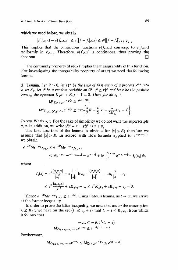
Iff is an arbitrary function in 9,+ ,(Ed+ ,), we take a sequence of smooth functions f, with compact support so that 1 1 f -fn~~,+,,,,+, + 0. Using the property of the magnitude of the difference between the upper bounds,
4. Limit Behavior of Some Functions
which we used before, we obtain
This implies that the continuous functions v(fn,s,x) converge to v(f,s,x) uniformly in E d + , . Therefore, v(f,s,x) is continuous, thus proving the theorem.
The continuity property of v(s,x) implies the measurability of this function. For investigating the integrability property of v(s,x) we need the following lemma.
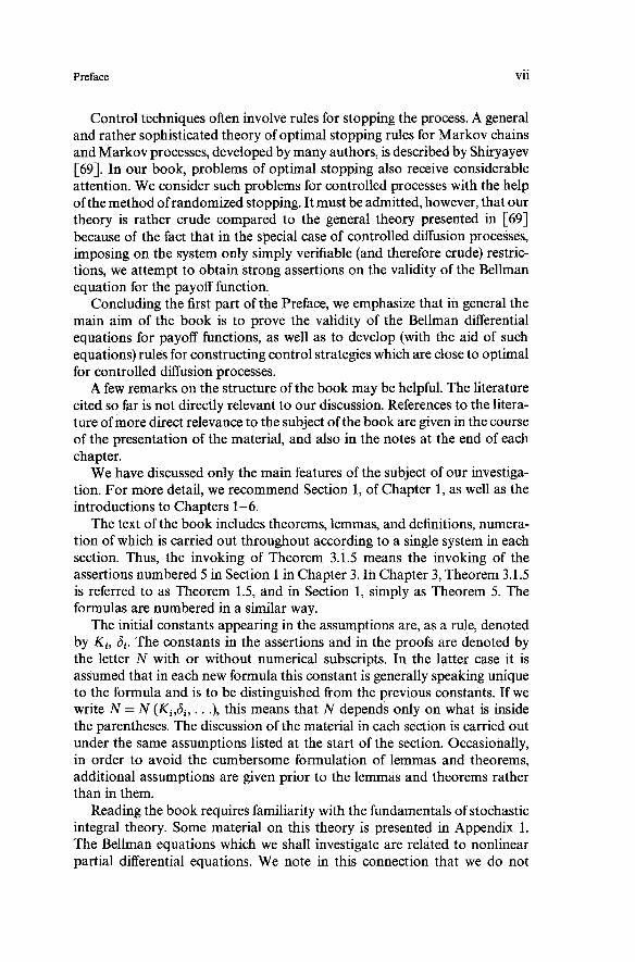
2. Lemma. Let R > 0, let ~2~ be the time ofjirst entry of a process x:3X into a set SR, let ya be a random variable on Qa, ya 2 72" and let E be the positive root of the equation K,E' + K,E - 1 = 0. Then, for all t,, s
rp;= < e & R ~ & l ~ l , M a x y u , ,e- -
PROOF. We fix a, x. For the sake of simplicity we do not write the superscripts a, x. In addition, we write y;ks = s + y;kO as s + y,.
The first assertion of the lemma is obvious for 1x1 < R; therefore we assume that 1x1 > R. In accord with Ito's formula applied to e-'t-Elxtl we obtain
where
Hence e - & R ~ e - r p q X , s t I e-"'"I. Using Fatou's lemma, as t -+ co, we arrive at the former inequality.
In order to prove the latter inequality, we note that under the assumption r, < K3ct we have on the set ( t , I y, + s} that t , - s I K3cp,, from which it follows that
Furthermore,

2 Auxiliary Propositions
Having multiplied the extreme terms in the last two inequalities we establish the second assertion of the lemma, thus completing the proof of the lemma.
3. Theorem. There exists a finite function N(d,Kl) increasing with respect K , and such that for all f E 9p + , (Ed + ,)
PROOF. Suppose that we have proved the theorem under the condition that K 2 = K 3 = 1. In order to prove the theorem under the same assumption in the general case, we use arguments which replace implicitly the application of the self-scaling property of a Wiener process (see Exercise 3.5).
If a E % = %(K1,K2,K3), let
1 1 rRa,Fa,Pa,&,wf,Ft, - a;, - b;,c;,
& 4 G It is seen that a' E % = %(K1/&,l,l). It is also seen that a' runs through the entire set % ( K 1 / G , 1 , 1 ) when a runs through the entire set %(Kl,K2,K3).
Further, for f E 9,. ,(Ed+ ,) let f '(t,x) = f (K3t,&x). We have
= sup M a Sow e-"@ f ( y ~ " , x ; , ~ ) dt a s %
- - K:/(P+ ' ) K ~ ( P + l ) sup M" Som e-@'+trf (s + K , y;',', x + G x ; ' , O ) dt a' E 'U'
Therefore, if we have proved our theorem for K2 = K3 = 1, then
11v(K1,K2,K3,fr',.)Il:zi,Ed+l
- - K:KP12)d S l ~ I ~ ( ~ , l , l , f l , s , x ) r l dxds

4. Limit Behavior of Some Functions
Therefore,it suffices to prove this theorem only for K , = K , = 1. We use in our proof in this case the expression
representable as the "sum" of terms each of which incorporates the change which occurs while the process (yr*",xy) moves across the region associated with the given term.
We assume without loss of generality that f 2 0. Let R be such that the volume of S, is equal to unity. We denote by w(t ,x)
the indicator of a set C,,,. Let At,,xt,(t,x) = w ( t , - t,xl - x)f( t ,x) . It is seen that
Ia(s,x) = S_" rn d t , f dx , Ma Som e-qF$x t,,,,, ( y ; + , x g dt.
In order to estimate the last expectation for fixed t , , x , , we note that At ,,,, )(t,x) can be nonzero only for 0 I t , - t I 1, Ix, - xl r R. Hence, if ya is the time of first entry of the process ( t , - yF%, - xFx) into the set C,,,, then
Furthermore, on the set {ya < co)
0 I t l - y;f I 1 and R 2 Ix, - x;kXI = IXY-~~I. The last inequality in the preceding lemma implies the inequality ya 2 z;*-"'. By Theorem 3.3 and the preceding lemma we obtain
E {4 2 1
I Ni(lAtl ,xl) l lp+i ,Ed+, exp - R - -1x - xll - - ( t i - s - 1) , 2 I where N , = N , ( d , K l , l ) is the constant given in Theorem 3.3. Also, we note that for t , < s the first expression in the above computations is equal to zero since t , - yFS I t l - s < 0 and ya = co. Hence
where .n(t,x) = exp[(&/2)R - (~/2)1x1 + +(t + I ) ] for t I 0, n(t,x) = 0 for t > 0. Therefore, since v = sup, I",

2 Auxiliary Propositions
In the right side of the last expression there is a convolution (with respect to (tl,xl)) of the two functions I l & t l , x l , I I P + l , E d + l and z(tl,xl). It is a well- known fact that the norm of the convolution in 9, does not exceed the product of the norm of one function in 9p and the norm of the other function in 9 , . Using this fact, we conclude that
To complete the proof of the theorem it remains only to show that the last constant N(d,Kl) can be regarded as an increasing function of K , .
Let
where the I l f l l p + i , ~ d + I
In addition,
upper bound is taken over all f E zp+ l(Edtl)such that > 0. According to what has been proved above, N(d,Kl) < m. the sets 'U increase with respect to K,. Hence v, R(d,K,) increase
with respect to K,. Finally, it is seen that Iv( f,s,x)l I v(l f l,s,x) and
IIv(K1,l,l,f,',')llp+l,Ed+l I R(d,Kl)llf llp+l.Ea+l.
The theorem has been proved.
We extend the assertions of Theorem 1 and 3 to the case where the func- tion f(t,x) does not depend on t. However, we do not consider here the process r,, as we did in the previous sections. Let
= sup Ma fow e-@(~f)(P-~)/P(det an1/Pg(x:,") dt. ae%(K1,K2,0)
4. Theorem. (a) Let g E Zp(Ed); then v(x) is a continuous function,
Iv(~)I N(d3K1,K2)11~IIp,Ed'
(b) There exists ajinite function N(d,K1) increasing with respect to K , and such that for all g E YP(Ed)
This theorem can be proved in the same way as Theorems 1 and 3.

4. Limit Behavior of Some Functions
We proceed now to consider the main results of the present section. Let numbers K > 0, 6 > 0 be fixed, and let each point (t,x) E Ed+ (X E Ed) be associated with some nonempty set 23(t,x) (respectively, 23(x)) consisting of sets a of type (1). Let 23 be the union of all sets 23(t,x), 23(x). We assume that a function ct(w) is bounded on 23 x [0,co) x UaSZa and that for all a E 23, U E [ o , ~ ) , O E aa, y E Ed
tr ot[at]* 5 K, r: = 1,
ICCJtl*yl 2 61~1.
It is useful to note that (2) can be rewritten as d 1
(a:y, y) = 1 (a:)"yiyj 2 2621y12, i , j= l
since (a:y, y) = +(o:(o;)*y,y) = 4 1 ($)*yI2.
5. Theorem. (a) Let 1 2 1, > 0, let Q c Ed+ ,, let Q be an open set, and let f E z p + I(Q),
Za = p , s ,x - - inf(t 2 O:(t + s,xFsX) 4 Q),
= sup M' J: e-qT-Uf(t + s, x ~ ~ ) dt. a s B(s,x)
Then ~ l I z ~ I p + i , a 5 N(d,K,J,Ao)llf l l p + l , ~ .
(b) Let A 2 1, > 0, let D c Ed, let D be an open set, and let g E Yp(D),
za = T~~~ = inf (t 2 0 : ~ : ' ~ 4 D),
zyx) = sup Ma f: e-q;-ug(x:,x) dt. a e B(x)
Then
PROOF. Since all eigenvalues of the matrix a: are greater than id2, det a: 2 2a62d.. From this, assuming that f"= I f lxQ, i?: = C: + A, @: = q ~ : + At and noting that i?: 2 1, we find
Iz"s,x)( I N(6)A" -p)l(p + l) SUP M' Jo e-qt -a( Fa ) (p-d)l(p+l) a e B(s,x)
x (r: det a:)ll(~+ly(y:,"x:,s) dt. It is seen that
K 1 tr aa < - i?:, and f < - z;. ' - 1 '-1
Therefore,

2 Auxiliary Propositions
which implies, by Theorem 3, that
thus proving assertion (a) of our theorem since
Proceeding in the same way, we can prove assertion (b) with the aid of Theorem 4. The theorem is proved.
6. Theorem. (a) Suppose that Q is a region in Ed+ ,, fl(t,x) is a bounded Borel function, f E 9,+ l(Q), 1 > 0,
Za = Za.s.x - - infit 2 O:(s + t, xpx) $ Q},
zA(s,x) = zA( f ,s,x)
= a ~ ' t ) ( s , x ) sup M a [ ~ ~ e - Q ~ - A y ( s + t , x ~ 3 d t + e - ~ ~ ~ - " ~ l ( s + ~ , ~ ~ ~ x ) 1 . Then, there exists a sequence 1, + co such that l,zL(s,x) + f (s,x) (Q-as.). (b) Suppose that D is a region in Ed, g,(x) is a bounded Borel function,
g E Tp(D) , 2 > 07 Z~ = z ~ , ~ = inf{t 2 O:xFx $ D},
Then, there exists a sequence 1, + co such that l,zAn(x) + g(x)(D-as.).
7. Theorem. (a) W e introduce another element in Theorem 6a. Suppose that Q' is a bounded region Q' c Q' c Q. Then I(1.z" f f l l p + l , Q , + O as 1 + co. If fl = 0, we can take Q' = Q.
(b) Suppose that in Theorem 6b D' is a bounded region, D' c B' c D; then 1112~" gllp,D' -' 0 as 1 -t co. If g1 = 0, we can take D' = D.
PROOF OF THEOREMS 6 AND 7. It was noted in Section 2.1 that the property of convergence with respect to an exterior norm implies the existence of a subsequence convergent almost everywhere. Using this fact, we can easily see that only Theorem 7 is to be proved.
PROOF OF THEOREM 7a. First, let fl = 0. We take a sequence of functions f" E CF(Q) such that 1 1 f" - f llp+l,Q + 0. It is seen that
11z"f7s,x) - f(s7x)l I 11z"f,s7x) - z"(f",s,x)l + Il.zA(f",s,x) - f"(s,x)l + If " (3 ,~) - f(s,x)l,
4. Limit Behavior of Some Functions
from which, noting that Iz"(f;s,x) - z" f ",s,x)l I z"(J f - f"l,s,x), we obtain, in accord with Theorem Sa,
In the last inequality the left side does not depend on n; the first and third terms in the right side can be made arbitrarily small by choosing an appro- priate n. In order to make sure that the left side of the last inequality is equal to zero, we need only to show that for each n
In short, it suffices to prove assertion (a) for fl - 0 in the case f E C:(Q). In conjunction with Ito's formula applied to f(s + t, X>~)I-~F-" for each
a E B(s,x), t 2 0 we have
where
Since a;, b:, c; are bounded, IL; f(t,x)l does not exceed the expression
Denoting the last expression by h(t,x), we note that h(t,x) is a bounded finite function; in particular, h E Zp+ ,(Q).
Using the Lebesgue bounded convergence theorem, we pass to the limit in (3) as t -+ co. Thus we have
f(s,x) = A M a sz e-ql-uf(s + t,xex) dt - Ma S: e - q ~ - * f L ~ ( s + t, x:,') dt,
which immediately yields

2 Auxiliary Propositions
In short, we have
which, according to Theorem 5a yields
1 I Nllhllp+l,Q lim - = 0,
A+m 1
thus proving Theorem 7a for fl E 0. In the general case
IAz" f ,s,x) - f (s,x)l I il sup ~~e-@'~-"'"l f l(s + za, x:,.) 1 a s5(s ,x )
where the exterior norm ofthe second term tends to zero; due to the bounded- ness of fl the first term does not exceed the product of a constant and the expression
+ il sup M e-'pF-"(s + t, xpx) dt - f (s,x) 1 a , Jr
Therefore, in order to complete proving Theorem 7a, it remains only to show that ]ln"lp+l,Qr -+ 0 as il -+ co for any bounded region Q' lying together with the closure in Q. To this end, it suffices in turn to prove that nA(s,x) -+ 0 uniformly on Q'. In addition, each region Q' can be covered with a finite number of cylinders of the type C,,,(s,y) = {(t,x): 1 y - xl < R, It - sl < r}, so that C,,,,,(s,y) c Q. It is seen that we need only to prove that n"t,x) -+ 0 uniformly on any cylinder of this type.
We fix a cylinder C,,,(s,y) such that C,,,,,(s,y) c Q. Let zs(x) = infit 2 0: I X - xpXl 2 R}. Finally, we denote by p( l ) the positive root of the equation il - pK - p2K = 0. Also, we note that for (t,x) E C,,,(s,y) we have za"*" 2 r A zf;c(x). Hence
,
Furthermore, by Lemma 3.23 the inequality
holds true. Therefore, the function n"t,x) does not exceed Ae-" + I(ch p(il)R)-I on C,,,(s,y). Simple computations show that the last constant tends to zero as A -+ co. Therefore, n"t,x) tends uniformly to zero on C,,(s,y). This completes the proof of Theorem 7a.
Theorem 7b can be proved in a similar way, which we suggest the reader should do as an exercise. We have thus proved Theorems 6 and 7.
In Lemma 3.2, one should take .c = 0, c, = 1.

5. Solutions of Stochastic Integral Equations and Estimates of the Moments
8. Corollary. Let f E 2,+ l(Q), f 2 0 (Q-as.) and for all (s,x) E Q let
inf Ma Sr e-qy(s + t, x;sx) dt = 0. a t B(s,x)
Then f = 0 (Q-as.).
In fact, by Theorem 2.4 the equality (4) still holds if we change f on the set of measure zero. It is then seen that for 2 2 0
inf Ma Sr e-qr-Ay(s + t, x:sX) dt = 0. a E 5(s,x)
Furthermore, for f1 = 0
A z(-f,s,x)= - inf Ma s r e - q ~ - " f (s + t, x?") dt. a E 5(s.x)
Therefore, za = 0 in Q and - f = lim,,, 2,zk = 0 (Q-as.).
5. Solutions of Stochastic Integral Equations and Estimates of the Moments
In this section, we list some generalizations of the kind we need of well- known results on existence and uniqueness of solutions of stochastic equa- tions. Also, we present estimates of the moments of the above solutions. The moments of these solutions are estimated when the condition for the growth of coefficients to be linear is satisfied. The theorem on existence and uni- queness is proved for the case where the coefficients satisfy the Lipschitz condition (condition (2)) .
We fix two constants, T > 0, K > 0. Also, we adopt the following notation: (w,,F,) is a dl-dimensional Wiener process; x, y denote points of Ed; a,, a,(x), F,(x) are random matrices of dimension d x dl; b,(x), &x), t,, 5; are random d-dimensional vectors; r,, h, are nonnegative numbers. We assume all the processes to be given for t E [O,T], x E Ed and progressively measurable with respect to {Fib If for all t E [O,T], w, x, y
we say that the condition ( 9 ) is satisfied. If for all t E [O,T], w, x
lla,(~)11~ I 2r: + 2K21x12,
we say that the condition (R) is satisfied. Note that we do not impose the condition ( 9 ) and the condition (R) on
o",(x), &(x). Furthermore, it is useful to have in mind that if the condition ( 2 ) is satisfied, the condition (R) will be satisfied for r, = Ilot(0)ll, hi = Ibt(0)l

2 Auxiliary Propositions
(with the same constant K) since, for example, IJat(x)I12 I 2110,(0)11~ + 211.t(x) - ~t(O)Il2.
As usual, by a solution of the stochastic equation
we mean a progressively measuable (with respect to {Ft}), process xt for which the right side of (1) is defined4 and, in addition, xt(w) coincides with the right side of (1) for some set SZ' of measure one for all t E [O,T], w E SZ'.
1. Lemma. Let x, be a solution of Eq. (1) for 5, = 0. Then for q 2 1
We prove this lemma by applying Ito's formula to the twice continuously differentiable function I x ~ ~ ~ and using the inequalities
2. Lemma. Let the condition (R) be satisjed and let x, be a solution of Eq. (1) for tt = 0. Then, for all q 2 1, E > 0, t E [O,T]
where A = 4qK2 + E - A,,,. If the condition (9) is satisjed, one can take in (2) hs = lbs(0)l, rs = llcs(O)ll.
PROOF. We fix q > 1, E > 0, to E [O,T]. Also, denote by $(t) the right side of (2). We prove (2) for t = to. We can obviously assume that $(to) < co. We make one more assumption which we will drop at the end of the proof. Assume that xt(w) is a bounded function of w, t.
Using the preceding lemma and the condition (R), we obtain
Next, we integrate the last inequality over t. In addition, we take the expectation from the both sides of this inequality. In this case, the expectation of the stochastic integral disappears because, due to the boundedness of
Recall that the stochastic integral in (1) is defined and continuous in t for t I T if

5. Solutions of Stochastic Integral Equations and Estimates of the Moments
xt(o), finiteness of $(to), and, in addition, Holder's inequality,
M J: ~ x , l * ~ ~ o ( x , ) x ~ ~ t s NM J: llor(xt)llz dt '
Furthermore, we use the following inequalities:
P 1 5 - MIX,^^^ + 2 28
~ I ~ ~ 1 ~ q - ~ r : I MIX^^^^)' -(l/q)(~r:q)l/q.
Also, let
In accord with what has been said above for t 5 to,
m(t) I Ji [lqm(s) + w1 -"~q'(s)] ds.
Further, we apply a well-known method of transforming such inequalities. Let 6 > 0. We introduce an operator F, on nonnegative functions of one variable, on [O,to], by defining
It is easily seen that F, is a monotone operator, i.e., if 0 I ul(t) I u2(t) for all t, then 0 5 F,ul(t) I F,uZ(t) for all t. Furthermore, if all the nonnegative functions u; are bounded and if they converge for each t, then limn,, F,un(t) = F, limn,, un(t). Finally, for the function v(t) = NeQt for all suffi- ciently large N and 6 I 1 we have F,u(t) I v(t) if t E [O,to]. In fact,
for
It follows from (3) and the aforementioned properties, with N such that m(t) I v(t), that m(t) I F,m(t) I . . . I F:m(t) I v(t). Therefore, the limit limn,, F:m(t) exists. If we denote this limit by v,(t), then m(t) I v,(t). Taking the limit in the equality F;+lm(t) = F,(F;m)(t), we conclude that v, = F,v,. Therefore, for each 6 E (0,l) the function m(t) does not exceed some non-

2 Auxiliary Propositions
negative solution of the equation
We solve the last given equation, from which it follows that v,(t) 2 6, v,(O) = 6, and
vb(t) = ilqv,(t) + gv; -'l/q'(t). (4)
Equation (4), after we have multiplied it by v$114)- (which is possible due to the inequality v, 2 6) becomes a linear equation with respect to v;Iq. Having solved this equation, we find v,1/4(t) = 6'14 + $(t).
Therefore, m(t) I ( # I q + ll/(t))q for all t E [O,to], 6 E (0,l). We have proved the lemma for the bounded x,(w) as 6 -+ 0.
In order to prove the lemma in the general case, we denote by z, the first exit time of xi from S,. Then xi ,,,(o) is the bounded function of (o,t), and, as is easily seen,
Therefore the process xi,,, satisfies the same equation as the process x, does; however, o,(x), b,(x) are to be replaced by x ,,,, o,(x), ~,,,,b,(x), re- spectively. In accord with what has been proved above, M 1 ~ , , , , 1 ~ ~ I [$(t)Iq. It remains only to allow R -+ co, to use Fatou's lemma, and in addition, to take advantage of the fact that due to the continuity of x, the time z, -, co as R -+ co. We have thus proved our lemma.
3. Corollary. Let fi llas112 ds < co with probability 1, and let z be a Markov time with respect to (9,). Then, for all q > 1
In fact, we have obtained the second inequality using Holder's equality. The first inequality follows from the lemma, if we take o,(x) = a,X,,,, b,(x) = 0, write the assertion of the lemma with arbitrary K, E, and, finally, assume that K 1 0, E 1 0. %
4. Exercise
In the proof of the lemma, show that the factor 2q in Corollary 3 can be replaced by unity.
5. Corollary. Let the condition (2) be satisfied, let xi be a solution of Eq. ( I ) , and let 2, be a solution of the equation
2, = e + J; ~ , ( z , ) ~ w , + J; %(x;)ds.

5. Solutions of Stochastic Integral Equations and Estimates of the Moments
Then, for all q 2 1, t E [O,T]
+ Ilos(as) - as(ns)112q) ds,
where p = 4q2K2 + q.
PROOF. Let y, = ( x , - 2,) - (5 , - 5). Then, as is easily seen,
in this case
satisfy the condition (9). From this, according to the lemma applied to the process y,, we have
+ 2(zq - 1)s ; e ( l ~ ~ ) * t - ~ ) [M~~o, (x , + t, - 5) - i?s(Ts)112q]1~q ds.
We raise both sides of the last inequality to the qth power. We use Holder's inequality as well as the fact that
Ibs(as + Ss - Es) - Ks(x"s)l I Ibs(% + Ss - f s ) - bs('s)l + lbs(x"3 - ~ s ( ~ s ) l
I K21Ss - 51 + IbS(ZS) - Es(ns)l, (a + b)¶ I 2q - '(aq + bq),
which yields
+ 22q-11bs(~s) - E s ( ~ s ) 1 2 4 + 2q(2q - 1 ) q 2 ~ q - ~ ~ ~ q 1 ( ~ - Q2q
+ P(2q - l)q22q- l llas(Ts) - Zs(Ts)112q] ds.
It remains to note that Ix, - T,l I lytl + ISt - & I , I x , - RtIzq I 22q-11~t12q + 22q-1) t t - z l 2 q , thus proving Corollary 5.
6. Corollary. Let the condition (R) be satisfied, and let x , be a solution of (1). Then there exists a constant N = N(q,K) such that for all q 2 1, t E [O,T]
' q < N M I C , I ~ ~ + NtqP'M S; [ICSIzq + h' + r:q]eN"-s)ds. M l ~ t l -
In fact, the process y, r x, - 5, satisfies the equation
dy, = o(yt + t J d w , + b(y , + S,)dt, Y O = 0,

2 Auxiliary Propositions
the coefficients of this equation satisfying the condition (R), however with different h,, r,, K. For example,
Ilo,(x + 5,)112 121: + 2K2[1x + ttll2 1 2r: + 4K214;,12 + 4K21xI.
Therefore, using this lemma we can estimate Mlyt12q. Having done this, we need to use the fact that I X , / ~ ~ I 22q-11ytl + 2'4-I IttI*
In our previous assertions we assumed that a solution of Eq. (1) existed , and we also wrote the inequalities which may sometimes take the form oo I oo. Further, it is convenient to prove one of the versions of the classical Ito theorem on the existence of a solution of a stochastic equation. Since the proofs of these theorems are well known, we shall dwell here only on the most essential points.
7. Theorem. Let the condition (2') be satisjed and let
Then for t T Eq. (1) has a solution such that M f r Ixtl2 dt < co. If x,, y, are two solutions of (I), then P {s~p , ,~ , ,~~ lx , - ytl > 0) = 0.
PROOF. Due to Corollary 5, MIX, - y,12 = 0 for each t. Furthermore, the process x, - y, can be represented as the sum of stochastic integrals and ordinary integrals. Hence the process x, - y, is continuous almost surely. The equality x, = y, (a.s.) for each t implies that x, = y, for all t (a.s.), thus proving the last assertion of the theorem.
For proving the first assertion of the theorem we apply, as is usually done in similar cases, the method of successive approximation. We define the operator I using the formula
Ix, = Ji os(xs) dw, + fi bs(xs) ds.
This operator is defined on those processes x, for which the right side of (5) makes sense, and, furthermore, this operator maps these processes into processes Ix, whose values can be found with the aid of the formula (5).
Denote by V a space of progressively measurable processes x, with values in Ed such that
It can easily be shown that the operator I maps V into V. In addition, it can easily be deduced from the condition (2) that
MIIx. - Iyt12 I aM Si lxs - ys12 ds,
where a = 2K2(1 + TK2). Let xjO) r 0, xj"") = 5, + Ixj") (n = 0,1,2, . . .). It follows from (6) that

5. Solutions of Stochastic Integral Equations and Estimates of the Moments
Iterating the last inequality, we find
Since a series of the numbers (Ta)"12(n!)-n12 converges, it follows from (7) that a series of functions xj"") - xj") converges in V. In other words, the functions xj"") converge in V, and furthermore, there exists a process x", E V such that Ilxj") - %,I[ - 0 as n -+ GO.
Further, integrating (6), we obtain
IIIxt - IytIl 5 aTIlxt - ill. (8)
In particular, the operator I is continuous in V. Passing to the limit in the equality I(x j"") - (5 , + Ix = 0, we conclude 112, - (5, + I%)[[ = 0 , from which and also from (8) it follows that I%, = I(( + I%), for almost all t, w. However, the both sides of this eqbality are continuous with respect to t for almost all w. Hence they coincide for all t at once almost surely. Finally, taking xi = 5 , + I%,, we have xi = 5, + I(< + I%)), = 5, + Ix, for all t almost surely. Therefore, x, is a solution of the primary equation, ( I ) , thus com- pleting the proof of the theorem.
8. Exercise
Noting that as(x) = [os(x) - as(0)] + us(0), prove that the assertions of the theorem still hold if M j: 1q,12 dt < co, where
We continue estimating the moments of solutions of a stochastic equation.
9. Theorem. Suppose the condition (2) is satisjied, xi is a solution of Eq. ( I ) , and 2, is a solution of the equation
Then, ij- the process 5, - z, is separable, the process x, - 2, is also separable, and for all q 2 1, t E [O,T]
M sup I x , - %,Izq I NeNiM sup It, - ? , I z q s 5 t s 5 f
where N = N(q,K) .
PROOF. It is seen that x, - x", is the sum of 5, - ti, stochastic integrals and Lebesque integrals. Both types of integrals are continuous with respect to t. Hence, the separability property of 5 , - 5 implies that xi - x", is separable, and in particular, the quantity sup,,, lxs - is measurable with respect to w.

2 Auxiliary Propositions
As was done in proving Corollary 5, the assertion of the theorem in the general case can easily be deduced from that in the case where 5, = 5; = - 2, = 0, FS(x) = 0, bs(x) = 0. It is required to prove in the latter case that
M sup lxs12q I Ntq-'eN'M Jd [b.(0)1~~ + 11~~~(0)11'~] ds. S $ t
(9)
Reasoning in the same way as in proving Lemma 2, we convince ourselves that it is possible to consider only the case with bounded functions x,(o) and to assume, in addition, that the right side of (9) is finite.
First, we prove that the process
is a submartingale. We fix c > 0 and introduce an auxiliary function of the real variable r using the formula q(r) = d m . Note that cp(lx1) is a smooth function on Ed. In conjunction with Ito's formula,
xtgt(x*) [ I I g , ( X t ) I 1 2 - I C T t * ( X t ~ 2 ] } dt + eK2tqf(/xtl) - dw,.
Ixt I IxtI Let us integrate the last expression over t from s, up to s2 2 s,, and also,
let us take the conditional expectation under the condition Fsl. In this case, the expectation of the stochastic integral disappears (see Proof of Lemma 2). In addition, we use the fact that since
bt(xt)xt 2 - Ibt(xt)l IxtI 2 - K21xtI2 - lb,(0)1 Ixtl, 0 I cpl(r) I 1, lrl I q(r).
then
Furthermore, cp" 2 0, r la:(xt)xt12. Therefore,
from which, letting E go to zero, we obtain, using the theorem on bounded convergence, M {)I,, 1 Fsl) 2 )I,,. Therefore )I, is a submartingale.
From well-known inequalities for submartingales (see Appendix 2) as well as Holder's inequality we have
M sup I x ~ ~ ~ ~ I M SUP yiq < 4 ~ 1 7 ~ ' ~ sst S $ t
< 4 . 224- l e 2 4 K 2 t ~ I X , 1 2 4 + 4 . 22q- le2qK2t Z q - 1 - t M Jd /bs(0)12q ds.

5. Solutions of Stochastic Integral Equations and Estimates of the Moments
It remains only to use Lemma 2 or Corollary 6 for estimating MIX,^^^, and, furthermore, to note that tae" 2 N ( ~ , b ) e ~ ~ ' for a > 0, b > 0, t > 0. The theorem is proved.
10. Corollary. Let the condition ( R ) be satisfied, and let xt be a solution of Eq. (1). Then there exists a constant N(q,K) such that for all q > 1, t E [O,T]
M sup lxS - P NP-'eNtM Si [1ts12q + h:'I + 121 d ~ . S l t
I f 5, is a separable process, then
M sup lxslzq 5 NM sup 1tt12q + ~ t ' - ~ e ~ ' M Si + h 2 + I : ~ ] ds. S l t sct
First, we note that the second inequality follows readily from the first expression. In order to prove the first inequality, we introduce the process y, = x, - 5,. It is seen that dy, = ot(yt + t,)dw, + bt(yt + <,)dt, yo = 0. In estimating yt it suffices, as was done in proving Lemma 2, to consider only the case where y,(co) is a bounded function. Similarly to what we did in proving our theorem above, we use here the inequality bt(y, + &)yt 2 - Kzly,12 - (K21tt1 + h,)ly,l, thus obtaining that the process
is a submartingale. From the above, using the inequalities for submartingales as well as
Holder's inequality, we find
M sup 1 y t 1 2 q P M SUP r:q 5 4 4 ~ ~ : ~ s s t S l t
For estimating Mly,12q, it remains to apply Lemma 2, noting that ot(x + t,), b,(x + t,) satisfy the condition ( R ) in which we replace r:, h,, K by r: + 2K21tt12, ht + K21tt1, 2K, respectively.
11. Corollary. Let Si IIosI12 ds < m (as.). Then for all q t 1
2q
M sup 1s: dasl 5 2q+ ~ ( 2 9 - I ~ P - ' M ~i llosl12q ds. S l t
This corollary as well as Corollary 10 can be proved by arguments similar to those used to prove the theorem. Taking as(x) = a,, b,(x) = 0, we have the process x, = yo a,dws. The proof of the theorem for K = 0 shows that lxtl is a submartingale. Hence fvl sup,,, I ~ ~ 1 ~ 4 1 MIX,(^^, which can be estimated with the aid of Corollary 3.

2 Auxiliary Propositions
12. Corollary. Let there exist a constant K , such that /la,(x)II + Ib,(x)I I K1(l + 1x1) for all t, o, x. Let x, be a solution of Eq. (1) for 5, = xo, where xo is a j xed point on Ed. There exists a constant N(q,K,) such that for all q 2 0, t E [07T1
M sup Ix, - xOlq I Ntqi2eNt(1 + I X ~ ~ ) ~ , S I t
M sup 1xSl4 5 ~ e ~ ' ( 1 + I X O ~ ) ~ , S S t
In fact, for q 2 2 these estimates are particular cases of the estimates given in Corollary 10. To prove these inequalities for q E [0,2] we need only to take
= sups5,(xs - x01(1 + l ~ o l ) - ~ , q2 = sup,,tlx,l(l + 1x01)- l and, further- more, use the fact that in conjunction with Holder's inequality, ~ l q , 1 ~ I ( M I V ~ I ~ ) ~ ~ ~ .
13. Remark. The sequential approximations x: defined in proving Theorem 7 have the property that
lim M sup Ix: - xtI2 = 0, n-tm t I T
where x, is a solution of Eq. (1). Indeed,
X : + ' = ( ~ + I X ; , x ,=t t+I j z t , x:+l-x ,=Ix:-I jZ, ,
from which, using Corollary 11 and the Cauchy inequality, we obtain
M sup Ix:" - xtl2 5 Z M sup [oS(x:) - as(Xs)] dw, t S T ,ST
+ 2M sup [bs(x:) - bs(ds)] ds t S T
T + NM SoT lbS(x:) - bs(K))12 ds 2 NM So Ix: - jz,12 ds.
As was seen in the proof of Theorem 7, the expression given above tends to zero asn -+ co.
6. Existence of a Solution of a Stochastic Equation with Measurable Coefficients
In this section, using the estimates obtained in Sections 2.2-2.5 we prove that in a wide class of cases there exists a probability space and a Wiener process on this space such that a stochastic equation having measurable coefficients as well as this Wiener process is solvable. In other words, ac-

6. Existence of a Solution of a Stochastic Equation with Measurable Coefficients
acording to conventional terminology, we construct here "weak" solutions of a stochastic equation. The main difference between "weak solutions and usual ("strong") solutions consists in the fact that the latter can be con- structed on any a priori given probability space on the basis of any given Wiener process.
Let o(t,x) be a matrix of dimension d x d, and let b(t,x) be a d-dimensional vector. We assume that a(t,x), b(t,x) are given for t 2 0, x E Ed, and, in addition, are bounded and Bore1 measurable with respect to (t,x). Also, let the matrix a(t,x) be positive definite, and, moreover, let
for some constant 6 > 0 for all (t,x), I E Ed.
1. Theorem. Let x E Ed. There exists a probability space, a Wiener process (w,,F,) on this space, and a continuous process x, which is progressively mea- surable with respect to {F,}, such that almost surely for all t 2 0
x, = x + Jd c(s,xS) dws + Ji b(s,xs) ds.
For proving our theorem we need two assertions due to A. V. Skorokhod.
2. Lemma.5 Suppose that dl-dimensional random processes 5: ( t 2 0, n = 0, 1,2, . . .) are dejined on some probability space. Assume that for each T 2 0, & > O
lim sup sup P { I ~ : I > C } = 0, c+m n f < T
lim sup sup ~{lt: , - 5:,1 > E } = 0. h 1 0 n t t , t z<T
I f ~ - t z l < h
Then, one can choose a sequence of numbers n', a probability space, and random processes 5, defined on this probability space such that all finite- dimensional distributions of 5":' coincide with the pertinent jinite-dimensional distributions of 5:' and P { I ~ ' - -,I > E } -+ 0 as n' -+ cc for a11 E > 0, t 2 0. 3. Lemma.6 Suppose the assumptions of Lemma 2 are satisfied. Also, suppose that dl-dimensional Wiener processes (w:,F:) are defined on the aforegoing probability space. Assume that the functions 5:(0) are bounded on [O,cc) x 52 uni$ormly in n and that the stochastic integrals 1: =yo 5: dw: are dejined. Finally, let 5: -t c:, w: -t w: in probability as n -+ co for each s 2 0. Then 1; -+ I: as n -+ co in probability for each t 2 0.
4. Proof of Theorem 1. We smooth out o, b using the convolution. Let on(t,x) = o('")(t,x), bn(t,x) = b( ' " ' ( t , ~ )~ (see Section 2.1), where E , -+ 0 as n -+ a,
See [70, Chapter 1, $61.
See [70, Chapter 2, $61. ' In computing the convolution we assume that oij(t, x ) = adi', b'(t, x) = 0 for t < 0.
2 Auxiliary Propositions
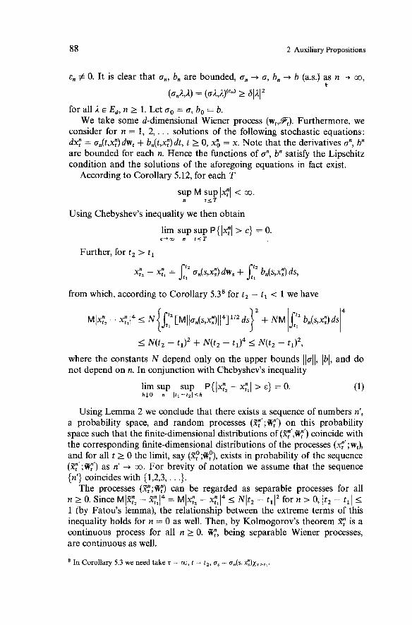
E, # 0. It is clear that on, bn are bounded, on -+ a, bn -t b (a.s.j as n + CO, c.
(onA,l) = (oA,l)(") 2 61A12
for all A E Ed, n 2 1. Let a, = o, bo = b. We take some d-dimensional Wiener process (w,,Ft). Furthermore, we
consider for n = 1, 2,. . . solutions of the following stochastic equations: dx: = on(t,x:) dw, + bn(t,x:) dt, t 2 0, x", x. Note that the derivatives on, bn are bounded for each n. Hence the functions of on, bn satisfy the Lipschitz condition and the solutions of the aforegoing equations in fact exist.
According to Corollary 5.12, for each T
sup M sup Ix:~ < CO. n t < T
Using Chebyshev's inequality we then obtain
lim sup sup ~{lx:l > C) = 0. c + m n t < T
Further, for t, > t,
xY2 - x:, = l2 on(s,xE) dws + J: bn(s,x;) ds,
from which, according to Corollary 5.38 for t, - t1 < 1 we have
where the constants N depend only on the upper bounds /loll, Ibl, and do not depend on n. In conjunction with Chebyshev's inequality
lim sup sup P {lx;, - x:,l > E) = 0. h10 n I t l - t z l < h
Using Lemma 2 we conclude that there exists a sequence of numbers n', a probability space, and random processes (x"y;l:') on this probability space such that the finite-dimensional distributions of (x":',~:') coincide with the corresponding finite-dimensional distributions of the processes (x:';~,), and for all t 2 0 the limit, say (x"P;CP), exists in probability of the sequence (x"?;C;') as n' -+ co. For brevity of notation we assume that the sequence {n') coincides with {1,2,3, . . .).
The processes (x":;C:) can be regarded as separable processes for all n 2 0. Since ~ lx" ; , - %;,I4 = MIX;, - x:,I4 4 NltZ - t1I2 for n > 0, ItZ - tll I 1 (by Fatou's lemma), the relationship between the extreme terms of this inequality holds for n = 0 as well. Then, by Kolmogorov's theorem x": is a continuous process for all n 2 0. C:, being separable Wiener processes, are continuous as well.
In Corollary 5.3 we need take z = co, t = t,, a, = a&. 4 ) ~ ,,,,.

6. Existence of a Solution of a Stochastic Equation with Measurable Coefficients
Further, we fix some T > 0. The processes (x;;w,) are measurable with respect to pT for t I T ; the increments w, after an instant of time T do not depend on F T . Therefore, the processes (x:;w,) ( t I T ) do not depend on the increments w, after the instant of time T. Due to the coincidence of finite-dimensional distributions, the processes (x":; f i : ) ( t 5 T ) do not de- pend on the increments C: after the time T for n 2 1. This property ob- viously holds true for a limiting process as well, i.e., it holds for n = 0. This readily implies that for n 2 0 the processes fi: are Wiener processes with respect to o-algebras of Fj"), defined as the completion of o(x":,C::s I t ) . Furthermore, for n 2 0 and each s I t the variable x": is Fj")-measurable. Since 2: is continuous with respect to s, 2: is a progressively measurable process with respect to {Fj")). These arguments show that the stochastic integrals given below make sense;
Let k-,(a) = 2-"[2"a], where [a] is the largest integer I a. Since o,(t,x";) for n 2 1 are bounded functions of (o , t ) , continuous with respect to t, and since k-,(t) - t as m -+ a, then
lim M Jb l l cn ( t , a - o n ( d t ) , + m . ) ) ~ ~ 2 dt - 0 m-t m
for n 2 1 for each T 2 0. Hence for each t 2 0
Writing similar relations for So a,(s,x:) dw,, Sfo b,(s,2:) ds, 6 b,(s,x3 ds, and using the fact that the familiar finite-dimensional distributions coincide, we can easily prove that for all n 2 1, t 2 0
In other words,
for each t 2 0 almost surely. We have thus completed the first stage of proving Theorem 1. If we had so far the processes xi, the convergence property of which we knew nothing about, we have now the convergent processes 2:. However, in contrast to x;, the processes 57: satisfy an equation containing a Wiener process which changes as n changes.
We take the limit in (2) as n -, co. For each no 2 1, we have
where o,,(s,x,) satisfies the Lipschitz condition with respect to (s,x). Hence llono(t2,x";2) - ~no(tl,x":l)ll N(lt2 - tll + - x":ll).

2 Auxiliary Propositions
In addition, by virtue of (1)
lim sup sup ~{llo,,(t2,Z~~) - a,,(t~,jZ,:)ll > 8 ) = 0. h 1 0 n I t z - t l l < h
From this it follows, according to Lemma 3, that the first term in (3) tends in probability to So ono(s,jzsO)d@,O. Therefore, applying Chebyshev's inequality, we obtain
We estimate the last expression. It is seen that
M j, If (s72;)l ds I etM J: e-'1 f(s,%;)1 ds 5 etM Jr e-.l f(~,z;)l ds.
Therefore, by Theorem 3A9
for n 2 1, where N does not depend on n. For n = 0 the last inequality as well holds, which fact we can can easily prove for continuous f taking the limit as n 4 co and using Fatou's lemma. Furthermore, we can prove it for all Bore1 f applying the results obtained in [54, Chapter 1, $21. Let w(t,x) be a continuous function equal to zero for t2 + 1x1' r 1 and such that w(0,O) = 1,0 I w(t,x) I 1. Then, for R > 0
% M Ji (la. - anol/2(~,Z;) ds 5 NM Ji [I - w (+,;)I ds n-t w
+ E n-r rn M J ~ ~ ( A ~ ) R ' R
+ Nil lloo - ~nol1211d+~,~R,R.
It should be noted that f(a,cr:i) = ilo:A12 2 i621A12 since 61112 I (a,i,A) = (i,a:A) 5 111 (cr:ll.

7. Some Properties of a Random Process Depending on a Parameter
Estimating M Sb I I o , , - ~ ~ l l ~ ( r , n : ) dr in similar fashion, we find
for each no > 0, R > 0. Finally, we note that the last expression tends to zero if we assume first that no -+ oo, and next, that R + co. Therefore,
in probability. We have a similar situation for the second integral in (2). Therefore it follows from (2) that
for each t 2 0 almost surely. It remains only to note that each side of the last equality is continuous with respect to t ; hence both sides coincide on a set of complete probability. We have thus proved Theorem 1.
7. Some Properties of a Random Process Depending on a Parameter
In investigating the smoothness property of a payoff function in optimal control problems it is convenient to use theorems on differentiability in the mean of random variables over some parameter. It turns out frequently that the random variable in question, say J(p) , depends on a parameter p in a complicated manner. For example, J(p) can be given as a functional of trajectories of some process xf which depends on p. In this section we prove the assertions about differentiability in the mean of such or other functionals of the process.
Three constants T, K , m > 0 will be fixed throughout the entire section.
1. Definition. Let a real random process x , ( o ) be defined for t E [O,T]. We write x, E 2 if the process x , ( o ) is measurable with respect to ( o , t ) and for all q 2 1
We write x, E 2 B if x, is a separable process and for all q 2 1
M sup Ix,Iq < m. ,ST
The convergence property in the sets 2 , 2 B can be defined in a natural way.

2 Auxiliary Propositions
2. Definition. Let xp, x:, . . . , x;, . . . E 9 ( 9 B ) . We say that the 9-limit (9B-limit) of the process x: equals xp, and we write 9-limn,, x: = xp(9B-lim,,, x: = xp) if for all q 2 1
T lim M Jo ~x; - xplqdt = o lim M sup x: - xp/q = o). n+ m n + w t s T
Having introduced the notions of the 9-limit (9B-limit), it is clear what is meant by 9-continuity (9B-continuity) of the process xf with respect to the parameter p at a point p,.
3. Definition. Suppose that p , E Ed, unit vector 1 E Ed, yt E 9 ( 9 B ) . Further, suppose that for each p from some neighborhood of the point p , a process xp E 9 ( 9 B ) is given. We say that y, is an 9-derivative (9B-derivative) of xf at the point p, along the 1 direction, and also, we write
We say that the process xf is once 9-differentiable (9B-differentiable) at the point p , if this process xp has 9-derivatives (9B-derivatives) at the point p, along all 1 directions. The process xf is said to be i times (i 2 2) 9-differentiable (9B-differentiable) at the point p , if this process xp is once 9-differentiable (9B-differentiable) in some neighborhoodlo of the point p, and, in addition, each (first) 9-derivative (9B-derivative) of this process xf is i - 1 times 9-differentiable (9B-differentiable) at the point p,.
Definitions 1-3 have been given for numerical processes x, only. They can be extended to vector processes and matrix processes xi in the obvious way.
Further, as is commonly done in conventional analysis, we write yf =
9-(a/al)xf if yp" = 9 - ( a / a l ) ~ p l ~ = ~ , for all p , considered, 9-(dial, d1,)xp - 9-(a/al,)[9-(d/al,)xf], etc. We say that xp is i times 9-continuously 9-differentiable if all 9-derivatives of xp up to order i inclusive are 9- continuous. We shall not dwell in future on the explanation of such obvious facts.
We shall apply Definitions 1-3 to random variables as well as random processes, the former being regarded as time independent processes.
In order to grow familiar with the given definitions, we note a few simple properties these definitions imply. It is obvious that the notion of 9- continuity is equivalent to that of 9B-continuity for random variables. Furthermore, lMxP - MxP0l I MlxP - xPoI. Hence the expectation of an 9-
lo That is, at each point of this neighborhood.

7. Some Properties of a Random Process Depending on a Parameter
continuous random variable is continuous. Since
the derivative of MxP along the 1 direction at a point p, is equal to the expectation of the 9-derivative of xP if the latter exists. Therefore, the sign of the first derivative is interchangeable with the sign of the expectation. Combining the properties listed in an appropriate way, we deduce that (a/dl)MxP exists and it is continuous at the point p, if the variable xP is 9-continuously 9-differentiable at the point p, along the 1 direction. A similar situation is observed for derivatives of higher orders.
Since for z I T
X: is an 9-continuous variable if z(o) I T for all o , xp is an 9B-continuous process, and x: is a measurable function of o . A similar inequality shows that for the same z
if xp has an 9B-derivative along the 1 direction, and if x: and the right side of (1) are measurable functions of o. These arguments allow us to derive the properties of 9-continuity and 9-differentiability of the random variable x: from the properties of 2B-continuity and 9B-differentiability of the process xp. Furthermore, (1) shows that the order of the substitution oft for z and the order of the computation of derivatives are interchangeable.
Suppose that the process xp is continuous with respect to t and is 9 B - continuous with respect top at a point p,. Also, suppose that z (p) are random functions with values in [O,T], continuous in probability at the point p,. We assert that in this case x:&,, x:(,, are 9-continuous at the point p,. In fact, the difference IxS;",, - ~ : ? ~ ' ( " , , , 1 ~ -+ 0 in probability as p + p, and in addition, this difference is bounded by the summable quantity 2q-1 sup, IxpOlq. There- fore, the expectation of the difference indicated tends to zero, i.e., the variable x:tP, is 9-continuous. The 9-continuity of the second variable follows from the 9-continuity of the first variable and from the inequalities
In conjunction with Holder's inequality
M sup X: dS - J: X(" dS[ I M Ix: - x(" dS[ 2 Tq- M Jd Ix: - x("Iq ds. t < T

2 Auxiliary Propositions
Therefore, fi x!ds is an 9B-continuous process if the process xf is 2- continuous. We prove in a similar way that this integral has an 9B-derivative along the 1 direction, which coincides with the integral of the 9-derivative of xf along the 1 direction if the latter derivative exists. In other words, the derivative can be brought under the integral sign.
Combining the assertions given above in an appropriate way, we can obtain many necessary facts. They are, however, too simple to require formal proof.
It is useful to have in mind that if {Ff] is a family of a-algebras in 52 and if the process xf is k times 9-differentiable at the point p, and, in addition, progressively measurable with respect to {Ft-,), all the derivatives of the process xf can be chosen to be progressively measurable with respect to {Ff]. Keeping in mind that induction is possible in this situation, we prove the foregoing assertion only for k = 1. Let yf = 9-(a/al)xf. Having fixed p,
we find a sequence rn + 0 such that (l/r,)(~f+'~' - xp) -+ yp almost every- where dP x dt. Further, we take jj; = limn,, (l/r,)(xf+'"'x;) for those o, t for which this limit exists and jjf = 0 on the remaining set. It is seen that the process yf is progressively measurable. Also, it is seen that
since jjf = yf (dP x dt-as.). We shall take this remark into account each time we calculate 2-deriva-
tives of a stochastic integral. We have mentioned above that differentiation is interchangeable with the
(standard) integration. Applying Corollary 5.11, we immediately obtain that if (wf,Ff) is a dl-dimensional Wiener process, of is a matrix of dimension d, x dl, which is progressively measurable with respect to {Ft} and is 9-continuous at a point po, the integral 6 afdw, is 2B-continuous at the point p,. If of is 9-differentiable along the 1 direction at the point p,, then for p = po
A similar assertion is valid in an obvious way for derivatives of higher orders.
4. Exercise
Prove that if the function xf is continuous (continuously differentiable) with respect to p in the usual sense for all (t,w) and, in addition, the function M jrlxP1q dt(M j:l(a/ax)xfp dt for each I, 111 = 1) is bounded in some region for each q 2 1, the process xf is 9- continuous (9-differentiable and 9-(a/al)xf = (8lal)xf) in this region.

7. Some Properties of a Random Process Depending on a Parameter
Further, we turn to investigating the continuity and differentiability properties of a composite function. To do this, we need three lemmas.
5. Lemma. Suppose that for n = 1,2, . . . , t E [0, T I , x E Ed, the dl-dimen- sional processes x: measurable with respect to (w,t) are dejined, and, in addition, the variables h:(x) measurable with respect to (w,t,x) are given. Assume that x; -+ 0 as n -* co with respect to the measure dP x dt, and that the variable h:(x) is continuous in x for all n, w, t. Furthermore, we assume that one of the following two conditions is satisjied:
a. for almost all (w,t)
lim lim wr(6) = 0, 6-0 n-m
where w:(4 = suplxl sSlh:(x)l; b. for each E > 0
lim ii;;; JOT P { w : ( ~ ) > E } dt = O. S+O n-m
Then Ih:(x:)l I w;(lx;l) + 0 as n -+ co in measure dP x dt.
PROOF. We note that since h:(x) is continuous in x,w:(6) will be measurable with respect to (w,t). Further, condition (b) follows from condition (a) since (a) implies that wy(6) + 0 as n -+ co, 6 -+ 0 almost everywhere; (b) implies the same although with respect to dP x dt.
Finally, for each E > 0, 6 > 0
where the first summand equals zero by assumption. Thus, letting 6 + 0 and using (b), we have proved the lemma.
6. Lemma. Let x; be dl-dimensional processes measurable with respect to (co,t) (n = 0,1,2, . . . , t E [O,T]), such that 9-limn,, x: = xp. Let f,(x) be random variables dejined for t E [O,T], x E Ed, measurable with respect to (w,t), continuous in x for all (o,t), and such that If;(x)l 5 K(l + 1x1)" for all a, t, X . Then 9-limn+, f,(x:) = f(xp).
PROOF. First we note that under the condition ( f , (x ) ( I K( l + 1x1)" the processes f;(x:) E 9 for all n 2 0. Next, we write f;(x:) - f;(xP) as ht(y:), where ht(x) = f,(x + xp) - f,(xp), y: = x: - xp. Since MS:IJJ;I dt + 0, y: + 0 in measure dP x dt, from which we have, using Lemma 5 applied to y: and h,(x), that ht(y;) + 0 in measure dP x dt.
Since the function lal/(lal + 1) is bounded and

2 Auxiliary Propositions
in measure dP x dt, then for each q 2 1
lim M JOT lg/9:12q dt = 0. n-t m
(2)
Moreover, in view of the estimate If,(x)l I K(l + 1x1)" and the fact that
we have sup M SoT lx:12qm dt < m,
n
sup M JoT(l + 1ht(y:)l)2qdt < SUP M SoT [ I + K(1 + / X : ] ) ~ n n
+ K(l + < CO.
Using the Cauchy inequality, we derive from (2) and (3) that
s lim (M J: Ig:12qdt)1'2 (M J:(I + Iht(y:)l)2q dt)li2 = 0 n-t w
for each q 2 1. The lemma is proved.
We note a simple corollary of Lemma 6.
7. Corollary. If for n = 0, 1,2, . . . the one-dimensional processes xi, y: are dejined and 9-limn,, x; = xp, 9-limn,, y: = yp, then
Indeed, the two-dimensional process (x:,y:) has the 9-limit equal to (xp,yp). Furthermore, the function f(x,y) = xy satisfies the growth condition If (x,y)I I (1 + d m ) ' . Hence 9-limn,, f (x;,y;) = f (xp,yp).
8. Lemma. Suppose that the assumptions of Lemma 6 are satisfied. Also, suppose that for n = 1,2, . . , u E [0,1] the dl-dimensional random variables x:(u) are dejined which are continuous in u, measurable with respect to (o,t) and such that (x:(u) - xpI I Ix: - xpI. Then
Y-lim So1 ~ ( x : ( u ) ) du = ~ ( x p ) . n-t m
PROOF. In accord with Holder's inequality, for q 2 1

7. Some Properties of a Random Process Depending on a Parameter
It follows from the inequalities Ix:(u) - xPI < Ix : - X ~ I , Ix:(u)l I I x ; I + I x : - xPI that x:(u) E 3 and 2'-limn,, x;(u) = x; for each u E [0,1]. There- fore, by Lemma 6
In(4 - M JOT I f , ( d ~ ) ) - f,(x;) 1' dt + 0.
Finally, by the inequalities
we have that the limiting expression in (4) belongs to 3, and the totality of variables I,(u) is bounded. By the Lebesgue theorem, as n + co
thus proving the lemma.
Further, we prove a theorem on continuity and differentiability of a composite function.
9: Theorem. Suppose for x E Ed, and p in a neighborhood of a point po E Ed the random processes xp = xp(o), J (x ) = f,(o,x) with values in Ed and El, respectively, are given for t E [O,T] and measurable with respect to (t,o).
(a) For all t , o let the function f,(x) be continuous in x, let If,(x)( I K(l + IxI)", and let the process xp be 3-continuous at po. Then the process ft(xf) is also 9-continuous at po.
(b) Suppose that for all t ,o the functionf,(x) is i times continuously differenti- able over x. Furthermore, suppose that for all t, o the absolute values of the function f,(x) as well as those of its derivatives up to order i inclusively do not exceed K(l + 1x1)". Then, if the process xp is i times (2'-continuously) 3- differentiable at the point p,, the process ft(xp) is i times (2'-continuously) 2'-differentiable at the point po as well. In addition, for the unit vector 1 G Ed
where
for those i, p for which the existence of the left sides of (5) and (6) has been established.
PROOF. For proving (a) it suffices to take any sequence of points pn -+ p,, to put xj"' = xp" an4 finally, to make use of Lemma 6.
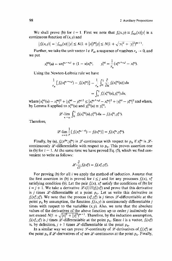
2 Auxiliary Propositions
We shall prove (b) for i = 1. First we note that ft(x,y) -f,(,,(x)lyl is a continuous function of (x,y) and
Ift(x,~)I = Iftcy)(x)I lyl I ~ ( 1 + IX~)~IYI I ~ ( 1 + J m l r n + ' .
Further, we take the unit vector 1 E Ed, a sequence of numbers r, + 0, and we put
Using the Newton-Leibniz rule we have
where Ixj")(u) - xPl2 + lyjn) - yp"12 I IxpO+rnl - xp"lZ + lyjn) - yp"12 and where, by Lemma 8 applied to xj")(u) and yj")(u) E yj"),
Therefore,
Finally, by (a), f,(xPO,ypO) is 9-continuous with respect to po if xpO is 9- continuously 9-differentiable with respect to p,. This proves assertion one in (b) for i = 1. At the same time we have proved Eq. (5), which we find con- venient to write as follows:
For proving (b) for all i we apply the method of induction. Assume that the first assertion in (b) is proved for i I j and for any processes ft(x), xf satisfying condition (b). Let the pair ft(x), xf satisfy the conditions of (b) for i = j + 1. We take a derivative 9-(a/al)ft(xp) and prove that this derivative is j times 9-differentiable at a point po. Let us write this derivative as fr(xf,yf). We note that the process (xf,yf) is j times 9-differentiable at the point po by assumption, the function ft(x,y) is continuously differentiable j times with respect to the variables (x,y). Also, we note that the absolute values of the derivatives of the above function up to order j inclusively do not exceed N(l + J m ) r n + l . Therefore, by the induction assumption, fr(xf,yf) is j times 9-differentiable at the point p,. Since 1 is a vector, ft(xp) is, by definition, j + 1 times 9-differentiable at the point p,.
In a similar way we can prove 9-continuity of 9-derivatives of ft(xf) at the point po if 9-derivatives of xf are 9-continuous at the point po. Finally,
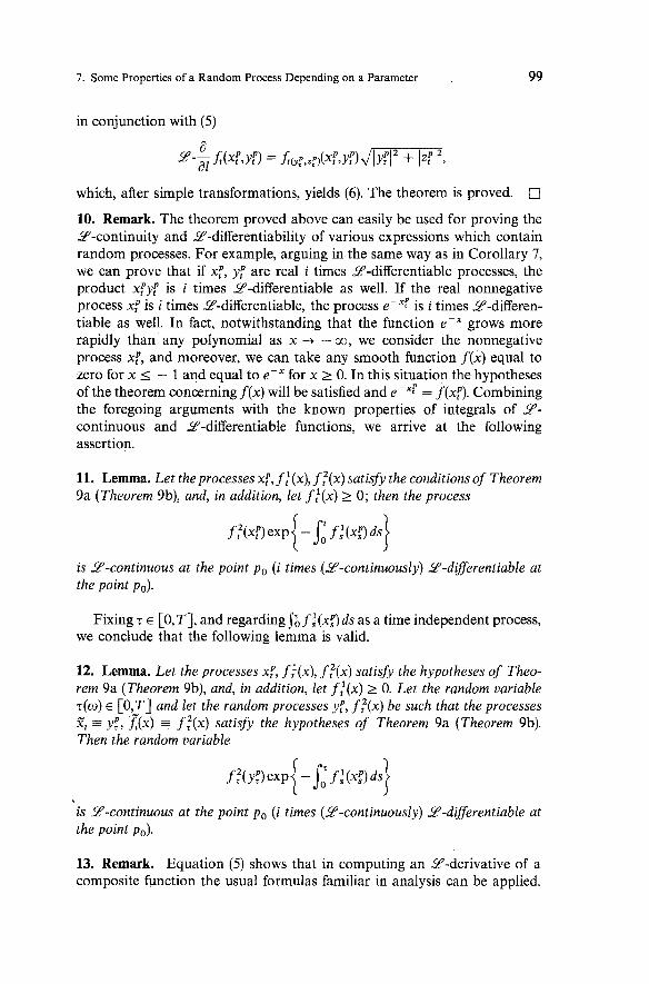
7. Some Properties of a Random Process Depending on a Parameter
in conjunction with (5)
which, after simple transformations, yields (6). The theorem is proved.
10. Remark. The theorem proved above can easily be used for proving the 9-continuity and 9-differentiability of various expressions which contain random processes. For example, arguing in the same way as in Corollary 7, we can prove that if xf, yf are real i times 9-differentiable processes, the product xfyf is i times 9-differentiable as well. If the real nonnegative process xp is i times 9-differentiable, the process e-"4 is i times 9-differen- tiable as well. In fact, notwithstanding that the function e-" grows more rapidly than any polynomial as x -r - co, we consider the nonnegative process xf, and moreover, we can take any smooth function f (x ) equal to zero for x I - 1 and equal to e-" for x > 0. In this situation the hypotheses of the theorem concerning f (x ) will be satisfied and e-"f = f (xf). Combining the foregoing arguments with the known properties of integrals of 9- continuous and 9-differentiable functions, we arrive at the following assertion.
11. Lemma. Let the processes xf, f :(x), f :(x) satisfv the conditions of Theorem 9a (Theorem 9b), and, in addition, let f :(x) 2 0; then the process
f : (x f) exP{- J; f :(.:I ds}
is 9-continuous at the point po (i times (9-continuously) 9-dgerentiable at the point p,).
Fixing z E [0, T I , and regarding S', f f (x f ) ds as a time independent process, we conclude that the following lemma is valid.
12. Lemma. Let the processes xf, f :(x), f :(x) satisfy the hypotheses of Theo- rem 9a (Theorem 9b), and, in addition, let f :(x) 2 0. Let the random variable z (o ) E [O,T] and let the random processes yf, f :(x) be such that the processes % = yf, x (x ) - f :(x) satisfy the hypotheses of Theorem 9a (Theorem 9b). Then the random variable
is 9-continuous at the point p, (i times (9-continuously) 9-diflerentiable at the point p,).
13. Remark. Equation (5) shows that in computing an 9-derivative of a composite function the usual formulas familiar in analysis can be applied.

2 Auxiliary Propositions
14. Exercise
Derive a formula for the derivative of a product, using (5). (Hint: Take a function f(x,y) = XY.)
We have investigated the properties of the functions f,(x:) in the case where f;(x) does not depend on n. We prove a few assertions for the case where f;(x) depends on the parameter n in an explicit manner.
15. Lemma. Let 5 ( 0 ) be a dl-dimensional random vector. Further, let h(x) = h(o,x), w(R,E) = w(o ,R ,~) be measurable variables which are dejined for x E Edl, R 2 0, E 2 0, p E Q. Assume that w(R,E) increases with respect to R and to E, Ih(x) - h(y)l I ~ ( 1 x 1 vlyl , I X - yl) for all o, X , y and (h(x)l I K(l + 1x1)" for all o, x. Then, for all R 2 0, E E (0,l)
PROOF. We fix R 2 0 , E E (0,1), and also we take a dl-dimensional vector q such that it does not depend on 5, w and is uniformly distributed in the sphere { X E Edl : 1x1 < 6).
It is seen that
Mlh(5)I M I ~ ( S ) I X I ~ I > R - ~
+ Mlh(5) - h(l + r ) l x l t ; l I R - l + Mlh(5 f v ) ~ x ~ I R - ~ .
The assertion of our lemma follows from the above expression as well as the assumptions of the lemma since < E < 1, for 151 I R - 1
15 + rl < R, - h(5 + r)( I w(R,E), and
Mlh(5 + v ) ~ x ~ ~ R - I
16. Lemma. Suppose that for x E Ed,, t E [O,T], n = 1,2,3, . . . , R > 0, E > 0 dl-dimensional processes x: are dejined which are measurable with respect to (o,t). Furthermore, suppose that the variables h:(x) and w:(R,E) increasing with respect to R and E are dejined, these variables being measurable with respect to (o,t,x) and (o,t), respectively. Assume that w:(lxl v I yl, I X - yl) 2 Ih:(x) - h:(y)l for all o, t, x, y,

7. Some Properties of a Random Process Depending on a Parameter
and for each R > 0,6 > 0
lim i& JOT P{w:(R,e) > 6 ) dt = 0. 810 n - t m
Finally, let h:(x) -+ 0 as n -+ oo in measure dP x dt for each x E E d . Then, h:(x:) + 0 as n -+ co in measure dP x dt.
We shall prove this lemma later. We derive from Lemma 16 (in the same way as we derived Lemma 6 from Lemma 5 ) the following theorem.
17. Theorem. Let the hypotheses of Lemma 16 be satisfied. Furthermore, let Ih:(x)I < K(l + 1x1)" for all n, w, t, x and for all q 2 1
Then
sup M JOT lx~~:lqdt < m. n
2- lim h;(x;) = 0. n+ m
18. Remark. By Chebyshev's inequality, (7) follows from (9). Using Che- byshev's inequality it can easily be proved that the condition (8) is satisfied if w:(R,E) is nonrandom and
lim JOT w~(R,E) dt = 0. 810 n - t m
For w:(R,E) it is convenient to take KE if Ih:(x) - h:(y)l < KIx - yl.
PROOF OF LEMMA 16. Since the convergence of h:(x:) to zero in measure is equivalent to the same convergence of (217~) arctan h:(x:), and furthermore, since the latter variable is bounded and
we can consider without loss of generality that Ih:l I 1. It is clear that in this case 2 A w: can be taken instead of w: so that w: will
be assumed to be bounded as well. According to Lemma 15 (we take in Lemma 15 K = 1, m = 0) for any
R > 0, E E (0,l)
We make use of the fact that the convergence in measure is equivalent to the convergence in the mean for uniformly bounded sequences. Thus we

2 Auxiliary Propositions
have that the sequence
as n - co for any y E Ed,. Furthermore, each term of this sequence does not exceed T. This implies that the last expression in (10) tends to zero as n - co for any E > 0, R > 0. Letting n + co in (lo), next, E 1 0, R + co, and in addi- tion, using (7), (8) and the fact mentioned above that the convergence in the mean and the convergence in measure are related, we complete the proof of Lemma 16.
8. The Dependence of Solutions of a Stochastic Equation on a Parameter
Let E be a Euclidean space, let a region D c E (D denotes a region of parameter variation), and let T, K, m be fixed nonnegative constants; (wt,Pt) is a dl-dimensional Wiener process. Furthermore, for t E [O,T], x E Ed, p E D, n = 0,1,2, . . . we are given: o,(x), o;(x), o,(p,x) are random matrices of dimension d x dl and b,(x), b:(x), b,(p,x), t:, t,(p) are random d-dimensional vectors which are progressively measurable with respect to {Pi). Assume that for all t , o, x, y
Also, assume that o:(x), b:(x) satisfy (1) for each n 2 0 and, in addition, ot(p,x), b,(p,x) satisfy (1) for each p E D.
Suppose that all the processes in question belong to 8 for all values of x, n, p. Recall that the space 8 was introduced in Section 7. We shall fre- quently use further on other concepts and results given in Section 7.
We define the processes x:, x:, xf as the solutions of the following equations:
x: = x + Jd os(x:) dw, + Ji bs(x;) ds;
x: = t: + Ji of(xS) dw. + J,' b:(xS) ds;
Note that by Theorem 5.7 the above equations have solutions. We also note that by Corollary 5.6 these solutions belong to 8. If t:, t,(p) E 2 B for all n, p, according to Corollary 5.10 x:, x:, xp E 8 B as well for all n, p, x.
1. Theorem. Let o:(x) - op(x), b:(x) - bp(x) in 8 as n - co for each x E Ed and let <: -+ 5: in 9 as n -, co. Then x: - x: in 8 as n + co.
If <: - tP in 8 B as well as n -+ co, then x; -+ x,O in 2 B as n - co.

8. The Dependence of Solutions of a Stochastic Equation on a Parameter
PROOF. Let 8:(x) = o:(x) - o:(O). It is seen that 8:(x) satisfies the Lipschitz condition (1) and the growth condition IlC:(x)II I KIxI. Furthermore, 8:(x) -r
8p(x) in 9 for all x. From this, using Theorem 7.17 and Remark 7.18, we conclude that C:(xp) + 8p(xp) in 9 . Adding the last relation with o:(O) -r
$(O) in 9 , we obtain: o:(xp) + op(xp) in 9 . Similarly, b:(x,O) -r bp(xp). Applying Corollary 5.5 and Theorem 5.9 for (%,i?,,b;) = (xp,op,bp),
(x,,o,,b,) = (x:,<,b:), we immediately arrive at the assertions of the theorem:
2. Corollary. If the process c,(p) is 9-continuous (9B-continuous), and, in addition, for each x E Ed the processes o,(p,x), b,(p,x) are 9-continuous in p at the point p, E D, the process xp is 9-continuous (9B-continuous) at the point po.
3. Lemma. Suppose that for each t E [O,T], p E D, w the functions o,(p,x), b,(p,x) are linear with respect to x. Let the process &(p) and for each x E Ed the processes oXp,x) and b,(p,x) be i times (9-continuously) 9-differentiable at the point p, E D. Then, the process xp is i times (9-continuously) 9- digerentiable at po. If, in addition, &(p) is i times (YB-continuously) 9 B - differentiable at the point p,, the process xf will be the same as the process 5,(~).
PROOF. Due to the linearity of o,(p,x), b,(p,x)
where (x:)j is the jth coordinate of the vector x: in the basis {ej). This implies that the last assertion of the lemma is a corollary of the first assertion as well as the results, which were proved in Section 7, related to the 9 B - differentiability of integrals and the 9-differentiability of products of 9- differentiable processes.
We prove the first assertion. To this end, we make use of the induction with respect to i and, in addition, assume that i = 1. We take a unit vector 1 E E and, in accord with what was said in Section 7, let the processes
be progressively measurable for x E Ed. By Corollary 2, we conclude that the process xp is 9-continuous at the
point p,. It is not hard to see that for p = p, the process

2 Auxiliary Propositions
exists, is progressively measurable (and 2-continuous with respect to p, if
are 2-continuous with respect to p). Furthermore, q,(p,) E 2 . According to Theorem 5.7, the solution of the equation
Y! = qt(p) + J,, ~ S ( P , Y ~ ~ W S + J ~S(P ,Y~) ds
exists and is unique for p = p,. Let us show that yp = 2-(d/dl)xp for p = p,. To this end, we take a
sequence rn -+ 0 and assume that yp(n) = r;'(~p+'~' - xp). It can easily be seen that
where
W e Z e given the expression
In addition, since the 2-limit of the product (sum) equals the product (sum) of 9-limits, we have that in 2 ,
Similarly, in 2
Thus, q,(p,,n) -+ qt(po) in T as n -+ co. Comparing (2) with (3), we have from Theorem 3 that ypO(n) -+ ypO in 2. Hence
for p = p,, proving thereby that xp is 2-differentiable. It is clear that (4) is satisfied at any point p at which there exist 2-deriva-
tives [,(p), at(p,x), bt(p,x). Further, if the foregoing derivatives are continuous

8. The Dependence of Solutions of a Stochastic Equation on a Parameter
at the point p,, they are defined in some neighborhood in which (4) is satisfied. In this case, as we noted above, q,(p) is 9-continuous at the point p,. Also, by Corollary 2; it follows from Eq. (2) that the process yf is 9- continuous at the point p,. This fact implies that the process xf is 9-con- tinuously 9-differentiable at p,.
Suppose that our lemma is proved for i = i, and that the assumptions of the lemma are satisfied for i = i, + 1. We shall complete proving our lemma if we show that each first 9-derivative of xf is i, times (9-con- tinuously) 9-differentiable at the point p,. We consider, for instance, 9-(d/dl)xf. This process exists and satisfies Eq. (2) for p close to po.
Since the assumptions of Lemma 3 are satisfied for i = i, (even for i = i, + I), by the induction assumption, the process xf is i, times (9- continuously) 9-differentiable at p,. From this, it follows that the process q,(p) is i, times (9-continuously) 9-differentiable at p,. Applying the in- duction assumption to (2), we convince ourselves that the process yf is i, times (9-continuously) 9-differentiable at the point p,. The lemma is proved.
4. Theorem. Suppose that the process &(p) is i times (9-continuously) 9- diferentiable at a point p, E D, and that the functions a,(p,x), b,(p,x) for each s, o are i times continuously (with respect to p, x) dzferentiable with respect to p, x for p E D, x E Ed. Furthermore, assume that all derivatives of the foregoing functions, up to order i inclusive, do not exceed K(l + 1x1)" with respect to the norm for any p E D, S, o, X. Then the process xf is i times (9- continuously) 9-difirentiable at the point po. If, in addition, the process &(p) is i times (9B-continuously) 9B-diferentiable at the point p,, the process xf will be the same as the process <,(p).
PROOF. Because the notion of the 9-derivative is local, it suffices to prove the theorem in any subregion D' of a region D, which together with its closure lies in D. We construct an infinitely differentiable function w(p) in such a way that w(p) = 1 for p E D', ~ ( p ) = 0 for p 4 D. Let &(p) = <,(p)w(p), iS,(p,x) = a,(p,x)w(p), E,(p,x) = b,(p,x)w(p). Then <,, E,, 5, satisfy the condi- tions of the theorem for D = E. Further, since the assertions of the theorem hold for 9, 3, 6 in Ej they hold as well for c, b, a in the region D'. This reasoning shows that in proving our theorem, we can assume that the assumptions of the theorem are satisfied for D = E.
In this case we use the induction over i. First, let i = 1. Further, we take a unit vector 1 E E and a sequence of numbers rn -, 0. Let
Using the Newton-Leibniz formula, we easily obtain

2 Auxiliary Propositions
where
We look upon the pair (p + urnl,x~(n,u)) as a process in E x Ed with a time parameter t . It is seen that
I(P + urn& x!(n,u)) - (p,x!)l I I(p + rnl, x!"~') - (p,x!)l.
Furthermore, by Corollary 2 and the 9-continuity of 9-differentiable functions, xpof *"' -+ XP in 9 . In order to apply Lemma 7.8, we note that, for instance, IbS,,,(p,x)l I K(l + d m ) " for all o, s, p, x. By this lemma, for p = po
in the sense of convergence in the space 9 in which
Note that Zs, &, v,, i7:, R, vt(p,n) are progressively measurable for those x, for which they exist. In fact, one can take the derivative 9-(a/al)<,(p) be progressively measurable. Also, for example, a,,,,(p,x) is progressively
measurable (ordinary derivative with respect to the parameter of a progres- sively measurable process) and continuous with respect to p, x. Hence the process ~ , , , ~ ( p + ur,l,x,P(n,u)) is progressively measurable and continuous with respect to u, which, in turn, implies the progressive measurability of the Riemann integral
J,l ~s,xj(p + w.1, x:(n,u)) du
and the progressive measurability of the process E:("(px).

8. The Dependence of Solutions of a Stochastic Equation on a Parameter
Further, since o,(p,x), b,(p,x) satisfy the Lipschitz condition (1) with respect to x, o,,,(p,x), b,,,,(p,x) are bounded variables. This implies that the functions 5,(p,x) and 6s(p,s), linear with respect to x, satisfy the Lipschitz condition (1). By Theorem 5.7, for p = p, there exists a solution of the equation
Y! = %(PI + J; ~S(P.Y:) dws + J; L(P.Y:) ds.
By Theorem 1, comparing (5) with (6), we conclude that
9- lim r; '(xf + *.' - xp) = 9- lim yf(n) = yf n-+ w n+ m
for p = p,. This shows that yp = 9-(a/al)xf for p = p,, and therefore the process xf is 9-differentiable at the point p,. It is also seen that yf = 9-(d/al)xf at each point p at which 9-(a/al)(,(p) exists.
Next, let (,(p) be 9-continuously 9-differentiable at the point p,. Then 9-(d/al)(,(p) exists in some neighborhood of the point p,, yp being the 9-derivative of xf along the 1 direction in this neighborhood. In addition, , the process (p,xp) is 9-continuous at the point p,, and the functions os,,,(p,x), b,,,,(p,x) are continuous with respect to (p,x) and do not exceed K(l + 1x1)" with respect to the norm. Therefore, by Theorem 7.9, the processes o,,,,(p,x:), b,,,,(p,x:) are 9-continuous, and consequently, the process y,(p) is 9- continuous at p,. Similarly, the fact that the functions o,,,,(p,x), b,,,,(p,x) are bounded and continuous with respect to p, x, implies that the processes Zs(p,x) and are 2-continuous at p, for each x. To conclude our reasoning, we observe that, by Corollary 2, the process yp interpreted as the solution of Eq. (6) is 9-continuous at the point p, .
Thus, we have proved the first assertion of the theorem for i = 1. Further, suppose that this theorem has been proved for i = i,, and, in addition, the assertions of the theorem are satisfied for i = io + 1. Consider the deriv- ative 9-(d/dl)xp. As was shown above, we may assume that this process is yp and that it satisfies Eq. (6). By the induction assumption, xp is i, times 9-differentiable at p,. Therefore the pair (p,xf) is i, times 9-differentiable as well. By Theorem 7.9, the processes r~,,,~(p,x:), b,,,,(p,x:), r~,,,~(p,x:), b,,,,(p,x:) are io times 9-differentiable at the point p,. Hence, in Eq. (6) the processes yt(p)LZs(p,x), 6s(p,x) are i, times 9-differentiable with respect to p. Since 5,(p,x), b,(p,x) are linear functions of x, according to the preceding lemma the process yp is i, times 9-differentiable at the point p,. We have thus proved that the derivative (a/dl)xp is i, times 9-differentiable at the point p,. Since 1 is an arbitrary unit vector from E, this implies, by definition, that xf is i, + 1 times 9-differentiable at the point p,.
In addition, if (,(p) is i, + 1 times 2-continuously 9-differentiable at the point p,, we can prove that xp is i, + 1 times 9-continuously 9- differentiable at the point p, if we put the word "9-continuously" in the appropriate places in the above arguments. This completes the proof of the first assertion of Theorem 4.

2 Auxiliary Propositions
For proving the second assertion of the theorem, we need only to prove, due to the equality
that the processes o,(p,xf), b,(p,xf) are i times (9-continuously) 9-differ- entiable at the point p,. It is obvious that a process which is identically equal to (p,O) is i times 9-continuously 9-differentiable. It is also seen that, since the function o,(p,O) is i times continuously differentiable with respect to p and, in addition, the derivatives of this function are bounded, the process o,(p,O) is i times 9-continuously 9-differentiable in accord with Theorem 7.9. Furthermore, the process (p,x:) is i times (9-continuously) 9-differentiable at the point p,, the function o,(p,x) - o,(p,O), with respect to the norm, does not exceed Klxl, and, in addition, the derivatives of this function satisfy the necessary restrictions on the growth. By Theorem 7.9, the process o,(p,x:) - o,(p,O) is i times (9-continuously) 9-differentiable at the point p,; the same holds for the process o,(p,x:) = o,(p,O) + [o,(p,x:) - o,(p,O)]. The process in b,(p,xf) can be considered in a similar way. The theorem is proved.
5. Remark. For i 2 1 we have proved that for any unit vector 1 E E the solution of Eq. (6) is the 9-derivative of xp along the 1 direction:
We have seen that the last equation is linear with respect to yf; also, we applied Lemma 3 to this equation for i 2 2. In Lemma 3 we derived Eq. (2), according to which the solution of the equation which follows is an 9- derivative of y! along the 1 direction, that is, a second 9-derivative of x! along the 1 direction. This equation is the following:
where, according to the rules of 9-differentiation of a composite function (see (2) ),

8. The Dependence of Solutions of a Stochastic Equation on a Parameter
Note that the above equations as well as equations for the highest 9- derivatives of xf can be obtained proceeding from the fact that xf is 9-differentiable the desired number of times, if we differentiate the equality
x! = <,(PI + J; os(~,x:) dws + J b,(p,x9 ds,
interchange the order of the derivatives with those of the integrals, and, in addition, make use of the formula for an 9-derivative of a composite function.
The following assertion is a simple consequence of Theorem 4 and Corollary 2 in the case where D = Ed, &(p) = p, at(p,x) = o,(x), b,(p,x) = b,(x).
6. Theorem. The process x: is 9B-continuous. If os(x), b,(x) are i times continuously differentiable with respect to x for all o, s, and iJ in addition, each derivative of these functions up to order i inclusively does not exceed K(l + 1x1)" with respect to the norm for any s, x, o, the process x: is i times 9B-continuously 9B-differentiable.
In concluding this section, we give two theorems on estimation ofmoments of derivatives of a solution of a stochastic equation. Since, as we saw in Remark 5, it was possible to write equations for such derivatives, it is reason- able to apply Corollaries 5.6 and 5.10-5.12 for estimating the moments of these derivatives. The reader can easily prove the theorems which follow.
7. Theorem. Let there be a constant K , such that for all s, x, p, w
Suppose that the process & ( p ) is 9B-differentiable at apoint p0 E D. Further, suppose that 9B-derivatives of the process & ( p ) have modijications which are progressively measurable and separable at the same time. Let the functions a,(p,x), b,(p,x) for each s, o be continuously differentiable with respect to p, x for p E D, x E Ed. In addition, let the matrix norms of the derivatives of the function a,(p,x) and the norms of the derivatives of the function bs(p,x) be smaller than K( l + 1x1)" (m 2 1) along all directions for all p E D, s, o, x. Then for any unit vector 1 E E, q 2 1, t E [O,T]
where N = N(q,K,m,K,).
8. Theorem. (a) Let the functions as(x), bs(x) be continuously differentiable with respect to x for each s, o. Then for any unit vector 1 E Ed, q 2 1, t E [O,T], X E Ed
s s t
where N = (q,K).

2 Auxiliary Propositions
(b) Let the functions o,(x), b,(x) be twice continuously dlfferentiable for each s, o. Further, for each x, s, o and unit vectors 1 E Ed let
Ilos(l,(l,(x)ll + Ibscl,cl,(x)l i K(1 + 1 ~ 1 ) ~ .
Also, suppose that IloS(x)II + Ib,(x)I I K l ( l + 1x1) for all x, s, o for some constant K,. Then for any q 2 1, t E [O,T], x E Ed and the unit vector 1 E Ed
where N = N(q,K,m,K,).
9. The Markov Property of Solutions of Stochastic Equations
The Markov property of solutions of a stochastic equation with non random coefficients is well known (see [9,11,24]). In this section, we shall prove a similar property for random coefficients of the equation (Theorem 4), and moreover, deduce some consequences from this property.
We fix two constants T , K > 0. In this section we repeatedly assume about (w,,F,), ti, ot(x), bt(x), with indices and tildes or without them, the following: (w,,F,) is a dl-dimensional Wiener process, o,(x) is a random matrix of dimension d x d l , b,(x), 5, are random d-dimensional vectors; ot(x), b,(x), 5, are defined for t E [O,T], x E Ed, progressively measurable with respect to { % I , and
for all possible values of the indices and arguments. We can now specify the objective of this section. It consists in deriving
formulas for a conditional expectation under the condition Fo of functionals of solutions of the stochastic equation
Note that if the assumptions made above are satisfied, in accord with Theorem 5.7 the solution of Eq. (1) on an interval [O,T] exists and is unique.
1. Lemma. Suppose that for all integers i, j > 0, t,, . . . , ti E [O,T], z,, . . . , z j E Ed the vector
{wtp, tip, otp(zq), btp(zq):p = 1, . . . , i, q = 1, . . . . j )
does not depend on Po. Then the process x,, which is a solution of Eq. ( I ) , does not depend on Fo either.
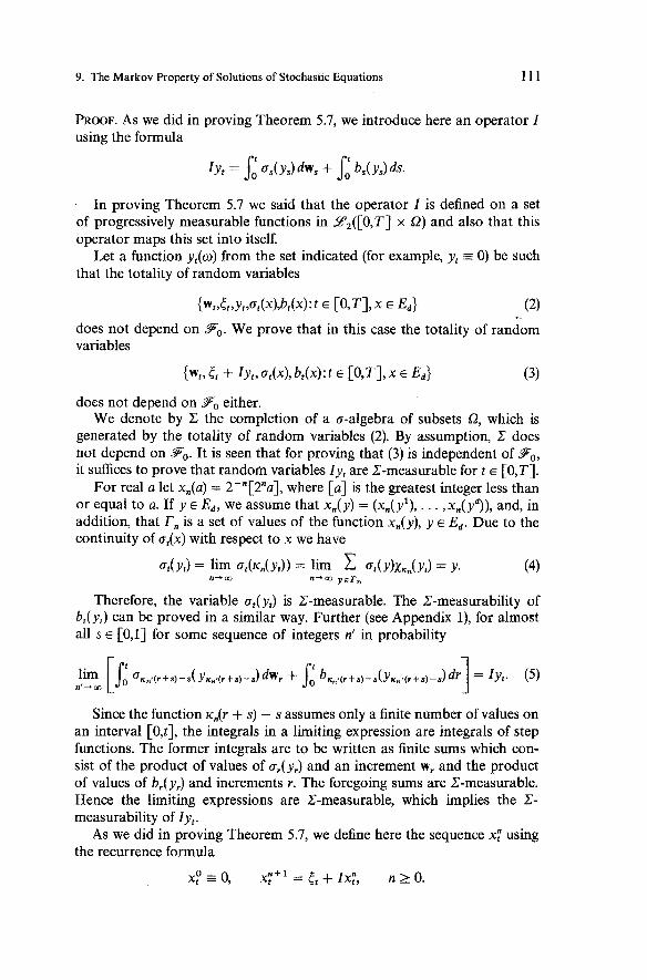
9. The Markov Property of Solutions of Stochastic Equations
PROOF. AS we did in proving Theorem 5.7, we introduce here an operator I using the formula
In proving Theorem 5.7 we said that the operator I is defined on a set of progressively measurable functions in LY2([0,T] x 52) and also that this operator maps this set into itself.
Let a function yt(w) from the set indicated (for example, yt = 0) be such that the totality of random variables
{wt,tt,~t,rrt(x),b~(x):t E [O,T], x E Ed) (2)
does not depend on Fo. We prove that in this case the totality of random variables
does not depend on Fo either. We denote by E the completion of a rr-algebra of subsets 52, which is
generated by the totality of random variables (2). By assumption, C does not depend on Fo. It is seen that for proving that (3) is independent of Po, it suffices to prove that random variables Iy, are C-measurable for t E [O,T].
For real a let xn(a) = 2-"[2"a], where [a] is the greatest integer less than or equal to a. If y E Ed, we assume that xn(y) = (xn(yl), . . . ,xn(yd)), and, in addition, that Tn is a set of values of the function xn(y), y E Ed. Due to the continuity of ot(x) with respect to x we have
Therefore, the variable ot(yt) is C-measurable. The C-measurability of bt(yt) can be proved in a similar way. Further (see Appendix I), for almost all s E [0,1] for some sequence of integers n' in probability
Since the function ~ , ( r + s) - s assumes only a finite number of values on an interval [O,t], the integrals in a limiting expression are integrals of step functions. The former integrals are to be written as finite sums which con- sist of the product of values of rrr(y,) and an increment wr and the product of values of br(yr) and increments r. The foregoing sums are C-measurable. Hence the limiting expressions are C-measurable, which implies the C- measurability of Iy,.
As we did in proving Theorem 5.7, we define here the sequence x: using the recurrence formula
2 Auxiliary Propositions
By induction, it follows from what has been proved above that the pro- cesses x: do not depend on Po for n 2 0, t E [O,T]. According to Remark 5.13, for t E [O,T]
1.i.m. x: = x,. n+ ao
Therefore, the process x, does not depend on P o . The lemma is proved.
In the next lemma we consider (i%,,@), 5",, E,(x), &(x) as well as (wt,Pt), St, ot(x), b,(x). AS we agreed above, we assume here that these elements satisfy the same conditions. Let x", be a solution of the equation
.', = + Si E~(.?.) d i~ , + Sd Er(zr)dr.
2. Lemma. Suppose that for all integers i, j > 0 and t,, . . . , ti E [O,T], z,, . . . , zj E Ed the following vectors are identically distributed:
Then the jinite-dimensional distribution of the process x, is equivalent to that of the process x",.
PROOF. We make use again of the operator I from the previous proof. Let
ifi = Ji cS(jjs) d ~ , + J', 6,(jjS) ds
and let the processes y,, jj, be progressively measurable with respect to {&I, (g}, respectively :
M Jd ly,/'dt < m, M Ji ~jj,~'dt < m.
Further, for any i, j > 0, t,, . . . , ti E [O,T], z , , . . . , zj E Ed let the vectors
have identical distributions. Note that if two random vectors have identical distributions, any (Borel) function of one vector has the same distribution as the other has. From this it follows, in accord with Eq. (4), that for any i, j > 0, t,, . . . , ti E [07T], z l , . . . , z j E Ed the vectors
~ w ~ ~ ~ S ~ ~ ~ Y ~ ~ ~ ~ ~ ~ ( Y ~ ~ ) ~ ~ ~ ~ ( Z ~ ) ~ ~ ~ ~ ( Y ~ ~ ) ~ ~ ~ ~ ( Z ~ ) : P = 1, . . . , i q = 1, . . . ,j),
{~zp,~tp,jjtp,~tp(jjzp),~fp(~q)7~tp(jjzp),b;p(~q):~ = 1, . . . ,i7 q = 1, . . . , j ) (7)
have the same distributions. It is useful to draw the reader's attention to the fact that in order to prove the proposition made above, we need to use vectors of type (6) at the values of z, different from those which appear in (7).
9. The Markov Property of Solutions of Stochastic Equations
We chooses E [0,1] SO that Eq. (5) holds for t = t , , . . . , ti, and, in addition, that similar representations hold for r. Having done this, we can see that the vectors
are representable as the limits in probability of identical functions of vectors of type (7). Therefore, the vectors (8) have identical distributions for any i,j > 0, t i , . . . , t i € [O,T], z,,. . . , z j € Ed.
Next, we compare the vectors (6) and (8). Also, we find sequences of the processes
Passing from vectors of type (6) to vectors of type (8), we prove by induction that the finite-dimensional distribution of x: is equivalent to that of 2:. Therefore, the finite-dimensional distributions of the limits of these processes in the mean square coincide, i.e., x, and j2;. The lemma is proved.
3. Corollary. If ti , a,(x), b,(x) are nonrandom and if, in addition, they are equal to c, F,(x), &x), respectively, for all t E [O,T], x E Ed, the processes x,, 2, have identical finite-dimensional distributions. Furthermore, the process x, does not depend on 9,, and the process jZ; does not depend on go.
This corollary follows from Lemmas 1 and 2 and the fact that all Wiener processes have identical finite-dimensional distributions and that, for example, w, = w, - w, does not depend on F0.
The formula mentioned at the beginning of the section can be found in the next theorem. In order not to complicate the formulation of the theorem, we list the conditions under which we shall prove the theorem.
Let Z be a separable metric space with metric p and let (w;,F:) = (wt,Ft), ob;(x), b;(x) be defined for z E Z. We assume (in addition to the assumption mentioned at the beginning of the section) that the functions o:(x,o), b:(x,o) are continuous with respect to z for all t , o , x and
for all x.
4. Theorem. Suppose that the assumptions made before proving the theorem are satisfied. Let the totality of variables
{w,,of(x),b:(x): t E [(),TI, x E Ed)
be independent of 9, for all z E Z. Further, let 5 be an 9,-measurable random variable with values in Ed and afinite second moment, let be an 9,-measurable

2 Auxiliary Propositions
random function with values in 2. Finally, let y, be a solution of the equation
W e denote by x:," a solution of the equation
Let F(Z ,X[ , ,~~) be a nonnegative measurable function on Z x C([O,T],Ed). Then
M { F ( ~ , ~ [ ~ , ~ ~ ) 190) = @(5,5) (a.s.), (1 1) where
cD(z,x) - MF(Z,XF$~).
PROOF. First we note that due to the conditions imposed, Eq. (9) and Eq. (10) are solvable and, in addition, are continuous with respect to t. Further, it suffices to prove Eq. (11) for functions of the form F(z,x,,, . . . ,x,,), where t i , . . . , tn E [O,T] and F(z,x,, . . . ,xn) is a bounded continuous function of (z,x,, . . . ,x,). In fact, in this case Eq. (11) extends in a standard manner to all nonnegative functions F(Z,X~,,,~), which are measurable with respect to a product of a o-algebra of Borel sets in z and the smallest a-algebra which contains cylinder sets of the space C([O,T],Ed). It is a well-known fact that the latter o-algebra is equivalent to the a-algebra of Borel sets of the metric space C( [O, T ] , E d ) .
In future, we shall consider functions F only of the type indicated. Let A = {z"); i 2 1) be a countable everywhere dense subset in Z . For z E Z we denote by R,(z) the first member of the sequence {z")) for which p(z,z(i) I 2-". It is easily seen that iS,(z) is the measurable function of z and that p(z,En(z)) 5 2-" for all z E Z. In addition, we define the function IC,(X)
as in the proof of Lemma 1. By Lemma 1, almost surely
where we take the limit as n -+ oo. We agreed to consider only bounded continuous functions F(Z,X[,,,~) (moreover, of special type). Hence, the left side of (12) yields the left side of (1 I ) , if we show that for some subsequence {n' >
lim sup Ix:n'"J3"n'(0 - y,l = 0 n ' 4 w t < T
In this case the right side of (12) yields the right side of (1 1) if we prove that @(z,x) is a continuous function of (z,x).

9. The Markov Property of Solutions of Stochastic Equations
Since the variables ~d i ) , K,(() are Fo-measurable, we can bring an indi- cator of the set {~,(i) = z, rc,(() = x) under the sign of a stochastic integral. Multiplying (10) by the indicator of the above set, bringing this indicator under the integral signs, replacing the values z, x by values En([), K,((), which are equal to z, x on the set considered, and, finally, bringing the indicator out, we have that on each set {En([) = z, rc,(c) = x) the process x ~ ~ ( ~ ) , ~ ~ ( ~ satisfies the equation
The combination of the sets {E,(i) = z, K,(() = x) with respect to z E A, x E r, produces all 52. Hence xKn(r)Kn(r) satisfies Eq. (14) on SZ. Comparing (9) with (14), we have in accord with Theorem 5.9 that
+ 1 lazn(5)( y,) - a$( y,) 1 1 '1 dt.
Here 15 - ~~((11 + 0 uniformly on 52, bp(r)(yt) -, bi(yt) for each t, due to continuity of b:(x) with respect to z. Furthermore, Ibp(i)(y,)12 + lb$(yJI2 does not exceed 4 sup, lbf(0)I2 + 4 ~ ~ 1 ytI2.
The last expression is summable over dP x dt. Investigating of(x) in a similar way, we conclude using the Lebesgue theorem that
This implies (13). For proving the continuity of @(z,x) with respect to (z,x) it suffices to prove that for any sequence (z,,x,) -+ (z,x) there is a sub- sequence (z,,,x,,) for which @(z,,,x,,) + @(z,x). From a form of @(z,x) we easily find that it is enough to have
lim sup lx;" ,xn' - xf,xl = 0 n'+m ,ST
The existence of such a subsequence {n') for any sequence (z,,x,) con- verging to (z,x) follows from the considerations which are very similar to the preceding considerations concerning Eq. (13). The theorem is proved.
5. Remark. The function MF(z,x;fT1) is measurable with respect to (z,x). Indeed, the set of functions F(z,x[,,~,) for which @(z,x) is measurable
contains all continuous and bounded functions F. For these functions F, @(z,x) is continuous even with respect to (z,x). From this we derive in a usual way that the set mentioned contains all nonnegative Bore1 functions F ( z , ~ [ ~ , ~ ] ) .

2 Auxiliary Propositions
6. Exercise
Prove that the assumptions of Theorem 4 about the finiteness of
can be weakened, and that it is possible to require instead uniform integrability of the values IJa:(0)112, I&(0)12 over dP x dt for z which run through each bounded subset Z.
Further, we consider the problem of computing a conditional expecta- tion under the condition 9,, where s E [O,T]. We shall reduce this problem to that of computing a conditional expectation under the condition go using a time shift. If the function F(xl0, T- ,] ) is defined on C([O, T - s], Ed) and xIo, ,-,] E C([O, T - s], Ed), we denote by F ( x [ , , ~ ~ ) a value of F on the function 0,x which is given by the formula (O,x), = x,+, for t E [0, T - s]. Sometimes F ( x [ , , ~ ~ ) is written as f3sF(x~o,T~,l). Similar notation can be used for the functions F(x[,,,,).
7. Theorem. Let the assumptions of Theorem 4 be satisjed. Further, let s E [O,T], and let ( = ( ( o ) , 5 = 5(o) be 9,-measurable variables with values in Z and Ed, respectively. Finally, let a:+,(x) and b:+,(x) be independent of o for all t 2 0.
Suppose the process y, satisjes the equation
for t E [s,T]. W e dejine the process xf3s*x for t E [0, T - s] as a solution of the equation
Then for any nonnegative measurable function F ( Z , X [ ~ , ~ - , ~ ) given on x C([O, T - sl, Ed),
{F([ ,~[s ,T]) 1 9s) = @(5,5) (a.s-), where ,
PROOF. Let G, = w, +, - w,, = % + ,, p, = y, +,, a:(x) = a;+ ,(XI, @(x) =.b:+ ,(x). It is seen that
in this case 5, L' are go-measurable, and G, is a Wiener process with respect to g. By Theorem 4
M T 1 9,) = F 0 - ] 1 go} = ( 1 (a.s.1,
9. The Markov Property of Solutions of Stochastic Equations
where $(z,x) = M F ( Z , ~ " ~ ~ ~ ~ - ~ , ) and Z:," is a solution of the equation
It remains to note that, by Corollary 3, the processes xf,"", x " $ s X have identical finite-dimensional distributions. Therefore $(z,x) = @(z,x), thus proving the theorem.
The technique involving a time shift can be applied in the case where s is a Markov time. The following fact, which we suggest the reader should prove using the above technique, leads to the so-called "strong Markovian" property of solutions of stochastic equations.
8. Exercise
Let a,(x) E a(x), b,(x) b(x) be independent of t and w, let z be a Markov time with respect to {Ft}, and let x: be a solution (it is given for each t ) of the equation
Prove that in this situation for any x E Ed and a nonnegative measurable function F = F(xlO,,)) given on C([O,w),E,),
M , { B , F I F ~ } = M,:F ( { z < a } - a s . ) ,
where x indicates that in computing the conditional expectation one needs to take xro,,, for the argument F, and x: indicates that first M,F - MF(X[~ , , , ) is to be found and, second, y is to be replaced by x:.
9. Remark. The assertions of Theorems 4 and 7 hold not only for nonnega- tive functions F. This property of F was necessary to make the expressions we dealt with meaningful. For example, Theorem 7 holds for any measurable function F for which ~ I ~ ( l , y [ , , ~ ) l < co. In fact, by Theorem 7
where @(, ,(z,x) = MF, (Z ,X~~," - ,~ ) . In this case the left side of (15) is finite with probability 1 for both the sign + and the sign - . In particular, the functions @(+,(z,x), @(-,(z,x) are finite for those (z,x) which are values of ([(o),((o)) on some subset S2 which has complete probability. Having subtracted from (15) with the + sign, the same with the - sign, we find
where @(z,x) = MF(z,~fb",',"-,~); in this case the function @(z,x) exists at any rate for those (z,x) which are necessary for Eq. (16) to be satisfied.
Theorem 7 enables us to deduce the well-known Kolmogorov's equation for the case where o,(x) and b,(x) do not depend on o .

2 Auxiliary Propositions
Denote by xFx a solution o f the equation
lo. Theorem. Let c,(x), f,(x), g(x) be nonrandom real-valued functions, c,(x) 2 0. Let ot(x), b,(x), c,(x), f,(x), g(x) be twice differentiable in x, where neither ot(x) nor b,(x) depends on w. Furthermore, let the foregoing functions and their first and second derivatives with respect to x be continuous with respect to (t,x) in a strip [O,T] x Ed. In addition, let the product of the functions at(x), b,(x), c,(x), f,(x), g(x) and their $rst and second derivatives and the function (1 + Ixl)-'" (functions and their derivatives) be bounded in this strip. Then the function v(t,x) has the following properties:
1. Iv(t,x)l I N(l + 1 ~ 1 ) ~ for all x E Ed, t E [O,T], where N does not depend on ( 4 4 ;
2. v(t,x) is once differentiable with respect to t7 is twice dzfferentiable with respect to x, and, in addition, the derivatives are continuous in the strip [O,Tl x Ed;
3. for all t E [O,T], x E Ed
Moreover, any function which has properties (1)-(3) coincides with v in the strip [O,T] x Ed.
PROOF. By assumption, Ilct(0)ll, Ibt(0)l are continuous. Therefore they are bounded on [O,T] and
where N does not depend on t, x. Furthermore, F(S ,X;$~- ,~) is a random variable since F(s,xI,, is a measurable (even continuous) function on

9. The Markov Property of Solutions of Stochastic Equations
C([O, T - s], Ed). From this and the assumptions If,(x)( l N(l + [XI)", Ig(x)I I N(l + 1x1)" and c,(x) 2 0 we deduce the first property of the func- tion v if we use estimates of moments of solutions of a stochastic equation (see Corollary 5.12).
Equation (17) makes sense, in general, only for t E [0, T - s]. It will be convenient to assume further that the process xs3" is defined for t E [O,T] for all s E (- c o , ~ ) , x E Ed. As before, we define the process x?" as a solution of Eq. (17), in which, having redefined the functions o,(x), b,(x) if necessary, we extend these functions from the interval [O,T] to (- co,co) defining ot(x) = crdx), b,(x) = bdx) for t 2 T and o,(x) = oo(x), bt(x) = b,(x) for t I 0. By Theorem 8.6, the process x?" is twice 9B-differentiable with respect to x. By virtue of the results obtained in Section 7 (see Lemmas 7.1 1 and 7.12), the above proves that the random variable F(S,X~&.-~,) is twice 9-differentiable with respect to x for each s E [O,T], and also that the function u(s,x) has all second derivatives with respect to x for each s E [O,T].
In order to prove that the function v(s,x) is continuous with respect to (s,x), we need only assume in (17) that p = (s,x), x = <,(p) , o,+,(y) = o,(p,y), bs+t(y) = ~,(P,Y), write cs+t(y) = ct(p,y), .L+t(y) = ~,(P,Y) in the expression for F, and, in addition, make use of Corollary 8.2 as well as the results from Section 7. Using similar notation, taking the first and second 9B-derivatives of xf3" with respect to x (see Remark 8.5), and the 9-derivatives of F ( x , s ~ ~ ~ - , ] ) and applying Corollary 8.2 as well as the results from Section 7, we prove that the first and second derivatives of v(s,x) with respect to x are continuous with respect to (s,x).
This implies continuity of Lv(s,x) + f,(x) with respect to (s,x). Hence, if the first relation in (18) has been proved, we have continuity of (a/dt)v(t,x). It should be mentioned that the second relation in (18) is obvious. Therefore, it remains only to prove that the derivative (a/at)v(t,x) exists and the first equality in (18) is satisfied. Furthermore, it suffices to prove this fact not for (d/at)v(t,x) but only for the right derivative of the function v(t,x) with respect to t for t E [O,T). Indeed, as is well known in analysis, if f(t), g(t) are continuous on [O,T] and if the right derivative f(t) is equal to g(t) on [O,T), then f '(t) = g(t) on [O,T]. We fix x and take t, > t,, t,, t, E [O,T]. Further, let s = t, - t,. By Theorem 7 (see Remark 9),
where @(y) = M F ( ~ , , X [ ~ , ~ ~ - ~ , ~ ) = v(t,,y). Furthermore, simple computations show that

2 Auxiliary Propositions
From this and (19) we find
where Y:'," - exp[-6 c,,+,(x:',")dr]. Next, let w(y) be a smooth function with compact support equal to 1 for
I Y - xl I 1. Also, let v,(t,,y) = v(t,,y)w(y), vz(t2,y) = v(t2,y) - Vl(t2,~). We represent the second term in (20) as the sum of two expressions starting from the equality u = v, f v,. Using Ito's formula, we transform the expression which contains v,. Note that derivatives of v,(t2,y) are continuous and have compact support, and therefore bounded. We have
where
It is seen that v = v, at a point x. We replace the expression vl(t2,x) in (21) by the expression v(t,,x) and carry the latter into the left-hand side of (21). Further, we divide both sides of the equality by s = t2 - t, and, in addition, we let t2 1 t,. By the mean-value theorem, due to continuity of the expressions considered
Moreover, \(l/s)h:',"l does not exceed the summable quantity
for some suitable values of the constant N, q. Finally, v,(t,,y) = 0 for 1 y - xJ I 1, and, by property 1, Iv2(t2,y)l I N(1 + 1~1)". Hence Iv~(t2,y)l I Nl y - ~ 1 " ' ~ and by Corollary 5.12,
The arguments carried out above enable us to derive from (21) that the right derivative of the function v(t,x) exists at a point t = ti, and also prove that the derivative equals [-J,(x) - Lv(t,,x)] for all ti E [O,T). As was explained above, this suffices to complete the demonstration of properties 1-3 for the function v.
We prove the last assertion of the theorem concerning uniqueness of solution of (18). Let u(t,x) be a function having properties 1-3. In accord

10. Ito's Formula with Generalized Derivatives
with Ito's formula for any R > 0
where zR equals the minimum of T - s and the first exit time of x:," from SR. It is seen that zR + T - s for R + oo. Moreover, the expression in the curly brackets under the sign of the last mathematical expectation in (23) is continuous with respect to zR and, in addition, it does not exceed a summable quantity of the type (22). Therefore, assuming in (23) that R + oo, using the Lebesgue theorem, we can interchange the sign of the limit and the sign of the expectation. Having done this and, further, having noted that u(T,x) = g(x), we immediately obtain u(s,x) = u(s,x), thus proving the theorem.
11. Remark. The last assertion of the theorem shows that v(s,x) depends neither on an initial probability space nor on a Wiener process. The function u(s,x) can be defined uniquely by the functions a,(x), b,(x), ~ ( x ) , f,(x), g(x), i.e., by the elements which belong to (18). The function v(s,x) does not change if we replace the probability space, or take another Wiener process, perhaps, even a d,-dimensional process with d, # dl, or, finally, take another matrix o,(x) of dimension d x d,, provided only that the matrix o,(x)of(x) does not change.
10. Ito's Formula with Generalized Derivatives
Ito's formula is an essential tool of stochastic integral theory. The classical formulation of the theorem on Ito's formula involves the requirement that the function to which this formula can be applied be differentiable a suffi- cient number of times. However, in optimal control theory there arises a necessity to apply Ito's formula to nonsmooth functions (see Section 1.5).
In this section, we prove that in some cases Ito's formula remains valid for functions whose generalized derivatives are ordinary functions. Moreover, we prove some relationships between functions having generalized deriva- tives and mathematical expectations. These relationships will be useful for our further discussion.

2 Auxiliary Propositions
W e fix two bounded regions D c Ed, Q c Ed+, in spaces Ed and Ed+,, respectively. Let dl be an integer, dl 2 d, let (w,,Ft) be a dl-dimensional Wiener process, let 0, = o,(o) be a matrix o f dimension d x dl , let b, = b,(o) be a d-dimensional vector, and, finally, let c, = c,(o) be real-valued. Further- more, let
Assume that o,, b,, c, are progressively measurable with respect t o {F , } and, in addition, for all t 2 0
Under the assumption made above, for each xo E Ed the process
is well-defined.
1. Theorem. Let s, x0 be jxed , xo E Ed, s E (- m,m). Also, let TQ be thejrs t exit time of the process (s + t, x,) from a region Q, let z be some Markov time (with respect to {F,}) such that z I z,, let z, be thejrs t exit time of the pro- cess x, from a region D, and, jnally, let z' be a Markov time not exceeding 2,. Suppose that there exist constants K , 6 > 0 such that Ilo,(o)II + Ibt(o)l + c,(o) 5 K , (a,A,A) 2 61;112 for all A E Ed and (o,t), which satisfy the inequality t < z V 2'.
Then for any u E W 2 ( 0 ) , v E W1,'(Q), t 2 0
+ r e-* grad, u(xr)or dwr,
+ S: e-+'r grad, v(s + r, xr)or dw, (1)
almost surely on the sets {z' 2 t } , { z 2 t ) , respectively. Furthermore, for any u 'E WZ(D), v E W1,'(Q)
u(xo) = - M J le -+ ' r~ru(xr ) dr + Me-qT'u(xr.),
10. Ito's Formula with Generalized Derivatives
PROOF. We prove both the assertions of Theorem 1 in the same way via approximation of u, v by smooth functions. Hence we prove the first assertion only.
Let a sequence vn E C1,2(&) be such that
I I v - v"IIB(Q) + 0, 112, - v"IIw~,~((L) + 07 lllgradx(v - vn)I211d+1,Q -) 0.
Further, let
Y, = xo + Ji ~r < P r dwr + Ji b < & r dr.
We note that y, = x, for t I z < co, which can easily be seen for t < r, and which follows from the continuity property of y, and x, for t = z < co. We prove that the right side of Eq. (1) makes sense. Obviously, for r < z
where N depends only on d, K. From this, using Theorem 2.4" we obtain
Similarly,
Nlllgradxv1211d+l,~. (3)
Further, we apply Ito's formula to the expression vn(t, yt)eCqt. Then, we have on the set {t I z) almost surely
e-q=vn(s + r, xJ - e-nvn(s + t, x,) = 1 e-*. (: + Lr) vn(s + r, x ) dr
+ 1 e-.. grad, vn(s + r, xr)or dwr. (4)
We pass to the limit in equality (4) as n + oo. Using estimates similar to estimates (2) and (3), we easily prove that the right side of (4) tends to the right side of (1).
The first assertion of Theorem 1 can be proved for the function u by an almost word-for-word repetition of the proof given. The slight difference is
'' In Theorem 2.4, we need take for D any region such that (- co,co) x D 3 Q.

2 Auxiliary Propositions
that if for vn the existence of the terms in (4) follows from the obvious bounded- ness of z(o) , then a similar formula for proving the first assertion of the theorem for u is valid since z f ( o ) < co ( a s ) and even Mz' < co (in Theorem 2.4, assume that s = 0, g = 1). The theorem is proved.
Henceforth, when we mention this theorem we shall call the assertions of the theorem Ito's formulas.
The assumption that the process x, is nondegenerate is the most restrictive assumption of Theorem 1. However, we note that the formulation of the well-known Ito formula imposes no requirement for a process to be non- degenerate when only differentiable functions are being considered. In the next theorem the assumption about nondegeneracy will be dropped, and in Ito's formula instead of an equality an inequality will be proved.
Consider the case where o,, b,, and c, depend on the parameter x E Ed. We fix s E E l . Furthermore, for t 2 s, x E Ed let there be given: o,(x), a random matrix of dimension d x d l ; bt(x), a random d-dimensional vector; c,(x) and f,(x), random variables. Assume that o, + ,(x), b, + ,(x), c, + ,(x), f,, ,(x) are progressively measurable with respect to {Ft) for each x, and that c,(x), f,(x) are continuous with respect to x and bounded for (w,t,x) E D x Q, where Q, as before, is a bounded region in Ed+ ,. Also, for all t 2 s, x and y E Ed let
Ilot(x) - ot(y)II + Ibt(x) - bt(y)l 4 Klx - Y I , 11ct(x)11 + Ibt(x)I K(1 + ] X I ) ,
where K is a constant. Under the above assumptions, for each x E E the solution xssx of the
equation
xt = x + Ji g s +r(xr) dwr + Ji bs + dr
exists and is unique (see Theorem 5.7). We denote by zr the first exit time of (s + t, x:") from the region Q ;
2. Theorem. Let (s,x) E Q and, in addition, let a function v E C(Q) belong to W1,2(Q') for each region Q', which together with its closure lies in Q. Assume that the derivatives of v can be chosen so that for some set r c Q, for which meas (Q\r) = 0, for all w and (t,y) E r the inequality

10. Ito's Formula with Generalized Derivatives
can be satisfied. Then for any Markov time z (with respect to (9,";) not exceeding
where cp, = cp;sx, xt = x ; , ~
PROOF. In proving Theorem 2, we drop the superscripts s, x. First, we note that in proving this theorem we can assume that z I zQ,, where Q' c Q' c Q. Indeed, for all such Markov times let our theorem have been proved. We take an arbitrary time z I 7,. It is seen that zQ, f zQ and z A zQP f z when the regions Q', while expanding, converge to Q. Substituting in (6) the variable z A zQ, for z, taking the limit as Q' f Q, and, finally, noting that v is continuous in Q, cp, and x, are continuous with respect to t, and, in addition, z and f,+,(xt) for t I z are bounded, we have proved the assertion of the theorem in the general case.
Thus, let z I ZQ,. Further, we apply a rather well-known method of per- turbation of an initial stochastic equation (see Exercise 1.1.1). We consider some d-dimensional Wiener process Kt independent of {Ft}. Formally, this can be done by considering a direct product of two probability spaces: an initial space and a space on which a d-dimensional Wiener process is defined.
We denote by x; a solution of the equation
x: = x + S, o,+.(x:) dw. + &.Et + fi b,+.(x;) dr,
where E, # 0, E , + 0 as n -+ a. It is convenient to rewrite the last equation in a different form. Let o:(x)
be a matrix of dimension d x (dl + d), such that the first dl columns of the matrix o:(x) form a matrix ot(x), and also the columns numbered dl + 1, . . . , dl + d form a matrix &,I, where I is a unit matrix of dimension d x d. Furthermore, we take a (dl + d)-dimensional Wiener process w, = (w:, . . . ,wfl, Kt, . . . ,Kf). Then
x: = x + Ji o;+.(x:) dm. + S; b,+,(x:) dr. (7)
By Theorem 8.1, sup ,,, Ix: - x,l + 0 as n + co in probability for each t. Therefore, there exists a subsequence ini} such that sup,,, Ix: - x,I + 0 (as.) as i + cc and for each t. In order not to complicate the notation, we assume that {nil = {n}.
Let z& be the first exit time of (s + t, x:) from Q'. It is not hard to show that limn,, 7;. 2 zQ, (as.). Hence, if we assume that
zi = z A inf z;,, nzi
then zi I z,, and zi -, z as i -+ co (as.). Further, we apply Theorem 1 to v, Q', x:, zi for n 2 i . Note that zi I z;
for n 2 i. Moreover, v E W1,2(Q'). Next, it is seen that

2 Auxiliary Propositions
where N does not depend on t, o, n. Finally,
All the assumptions of Theorem 1 have been satisfied. Therefore, com- puting for the process x: (see (7)) the operator L, appearing in Theorem 1, and in addition, assuming that
for n 2 i, we have
V(S,X) = -M S: e-"':g.+r(~;)dr + Me-p:iv(s + T ~ , X : ~ ) .
By the hypothesis of the theorem,
Furthermore, by Theorem 2.4,
Therefore, in integrating over r in the first expression in the right side of (8), we can assume that ( s + r, x:) E r. From (8) we find
- M S: e - ~ : AV(S + r, x:) dr. 2
Because zi does not exceed the diameter T of the region Q', sup,,, I x : - x , I + 0 as n + co, f ,+ , (y ) and c,+,( y) are continuous with respect to y, and zi t z as i + oo, we conclude that in the last expression for v(s,x) the first two terms in the right side as n + co, then as i + co, yield the right side of Eq. (6).
Therefore, for proving the theorem it remains only to show that
lim s:M ST IAv(s + r,x:)l dr = 0. n+ w
Making use of Theorem 2.2, we assume s = 0, c, = 1, F(c,a) = c, b, =
b,+,(x:), r, = 1, p = d, o, = cr:+,(x:). Note that, as was noted before, Ib,l 5

10. Ito's Formula with Generalized Derivatives
N . 1 = Nc, for t < z;l,, where N does not depend on n, and, moreover,
Therefore
where N does not depend on n. The last expression tends to zero as n + co, since v E W1?'(Q'). Therefore, the norm of that expression is finite. The theorem is proved.
3. Remark. It is seen from the proof that if for all ( t , o ) the function f,(x) is upper semicontinuous, lhxn,x f,(xn) 2 f , (x) , the assertion of the theorem still holds.
4. Corollary. If o,(x), b,(x), c,(x) do not depend on o and in addition, L,(x)v(t,x) + av(t,x)/at is a bounded continuous function of (t ,x) E Q, we have in the notation of the theorem
av V(S,X) = Me-..v(s + I ,XJ - M Sd e-* . L,+,(xr)u(s + r,xr) + - ( s + r,x.) dr.
az I 5. Exercise to Theorem 1
(Compare [44, p. 391.) Let d 2 2, a E (0,1), p = [(d - 1)/(1 - a)] - 1, u(x) = Ixla, b ( x ) = m, where aii(x) = 6" + p(xixj/lx12). We take as D a sphere S,, and also, we take as x, some (possibly "weak") solution of the equation dx, = o(xt)dw,, x , = 0 . Let o , = o(xt), b, = 0, C, = 0.
Show that second derivatives of u are summable with respect to D to the power p = ad/(2 - a). (Note that p -+ d as a -, 1.) Also, show that Lu(x,) = 0 (as.) and that Ito's formula is not applicable to u(x,).
6. Remark. In the case where Q = ( 0 ,T ) x S,, we have 7%'" = 0 for s = 0 in the notations introduced before Theorem 2. This suggests that it would be useful to have in mind that if Q = ( 0 ,T ) x S,, one can take in Theorem 2 instead of zs9" (in Theorem 1 instead of zQ) the minimum between T - s and the first exit time of the process xs,X (respectively, the first exit time of the

2 Auxiliary Propositions
process x,) from S,. For s = 0 this minimum is not in general equal to zero. Thus we can derive meaningful assertions from Theorems 1 and 2.
In order to prove the validity of the remark made above, it suffices to repeat word-for-word the proof of Theorems 1 and 2.
Notes
Section 1. The notations and definitions given in this section are of common usage. Definition 2 as well as the concept of an exterior norm are somewhat special.
Sections 2, 3,4. The results obtained in these sections generalize the corresponding results obtained in [32, 34, 36, 401. Estimates of stochastic integrals having a jumplike part can be found in Pragarauskas [62].
Sections 5, 7, 8, 9. These sections contain more or less well-known results related to the theory of Ito's stochastic integral equations; see Dynkin [Ill], Liptser and Shiryayev [51], and Gikhman and Skorokhod [24]. The introduction of the spaces Y , 9 B is our idea.
Section 6. The existence of a solution of a stochastic equation containing measurable coefficients not depending on time was first proved in [28] by the method due to Skorokhod [70]. In this section we use Skorokhod's method in the case when the coefficients may depend on time. For the problem of uniqueness of a solution of a stochastic equation as well as the problem of constructing the corresponding Markov process, see [24,28,38]; also see S. Anoulova and G. Pragarauskas: On weak Markov solutions of stochastic equations, Litovsky Math. Sb. 17(2) (1977), 5-26, also see the references listed in this paper.
Section 10. The results obtained in this section are related to those in [2f, 341.