Preface - imm.dtu.dk · 1.3 REPORT ROADMAP ... 5.1.4 Generating ALFP Logic Formulae ... This thesis...
149
i Preface This M.Sc. Thesis presents the results of my final master project entitled Static Analysis for Protocol Validation in Hierarchical Networks. The master project was carried out in the period of 18 th of January to 27 th of July 2005 and corresponds to 30 ETCS points. It has been the final part of my studies for the Master of Science degree at the Department of Informatics and Mathematics Modelling (IMM), Technical University of Denmark (DTU). I would like to take this opportunity to thank my supervisor, Professor Hanne Riis Nielson, for her counseling, support and not least her interest throughout the period of my M.Sc. Thesis project. I would also like to thank Flemming Nielson, Henrik Pilegaard, Terkel Tolstrup, Esben Heltoft Andersen and Christoffer Rosenkilde Nielson for comments and discussions during my thesis work. Last but not least, I would like to thank my wife, Shanshan Song, for her proof reading as well as emotional support. Lyngby, July 27 th , 2005 Ye Zhang
-
Upload
nguyenkhue -
Category
Documents
-
view
216 -
download
0
Transcript of Preface - imm.dtu.dk · 1.3 REPORT ROADMAP ... 5.1.4 Generating ALFP Logic Formulae ... This thesis...

i
Preface
This M.Sc. Thesis presents the results of my final master project entitled Static Analysis for Protocol Validation in Hierarchical Networks. The master project was carried out in the period of 18th of January to 27th of July 2005 and corresponds to 30 ETCS points. It has been the final part of my studies for the Master of Science degree at the Department of Informatics and Mathematics Modelling (IMM), Technical University of Denmark (DTU).
I would like to take this opportunity to thank my supervisor, Professor Hanne Riis Nielson, for her counseling, support and not least her interest throughout the period of my M.Sc. Thesis project.
I would also like to thank Flemming Nielson, Henrik Pilegaard, Terkel Tolstrup, Esben Heltoft Andersen and Christoffer Rosenkilde Nielson for comments and discussions during my thesis work.
Last but not least, I would like to thank my wife, Shanshan Song, for her proof reading as well as emotional support.
Lyngby, July 27th, 2005
Ye Zhang

ii

iii
Abstract
The ambient calculus presents a high-level view of mobile computation and gives rise to a high-level treatment of the related security issues. Ambients, which are named bounded places, allow us to model the concept of local networks in a natural way. The tree structure formed by ambients just captures the characteristic of our interested network, the hierarchical network. In this M.Sc. thesis, we focus on validating cryptographic protocols working on hierarchical networks. We begin with extending Boxed Ambients with annotations which declare the authentication intentions of cryptographic protocols. We then develop a static analysis for tracking the interested properties of a process. The analysis specification is defined in Flow Logic in order to separate the definition of specification from the actual implementation. Subject to the environment of the hierarchical network, we declare the capability of the attacker of the hierarchical network based on the Dolev-Yao attacker. The program analysis is fully implemented to compute least estimates for a process. Here we use the Succinct Solver as our constraint solver. It computes the least interpretation of predicate symbols given formulae written in Alternative-free Least Fixed Point logic (ALFP). With this tool, we validate symmetric key protocols applied on hierarchical networks. Keywords: Boxed Ambients, Static Analysis, Hardest Attacker, Flow Logic, Hierarchical Network, Cryptographic Protocol.

iv

v
Table of Contents
1 INTRODUCTION .........................................................................................................................1
1.1 MOTIVATION AND OBJECTIVES................................................................................................2 1.2 TECHNICAL CONTEXT OF FORMALISM.....................................................................................3 1.3 REPORT ROADMAP ..................................................................................................................4
2 ABOXED AMBIENTS..................................................................................................................5 2.1 PRINCIPLES: HIERARCHICAL NETWORKS VS. AMBIENTS ..........................................................5 2.2 SYNTAX ...................................................................................................................................7 2.3 SEMANTICS ............................................................................................................................10 2.4 ASSERTIONS FOR THE ORIGIN AND DESTINATION ..................................................................17 2.5 MODELING OF HIERARCHICAL NETWORKS............................................................................20 2.6 THE ABOXED AMBIENTS SPECIFICATION ..............................................................................21
3 CONTROL FLOW ANALYSIS.................................................................................................25 3.1 FLOW LOGIC IN ABOXED AMBIENTS .....................................................................................26
3.1.1 Semantic Correctness of the Ananlysis .............................................................................27 3.1.2 Succinct versus Verbose Flow Logics...............................................................................27
3.2 A CONTROL FLOW ANALYSIS FOR ABOXED AMBIENTS ........................................................28 3.2.1 Domain of the Control Flow Analysis ..............................................................................28 3.2.2 Definition of the Control Flow Analysis ...........................................................................30
3.3 CORRECTNESS OF THE ANALYSIS...........................................................................................35 4 MODELING THE ATTACKER................................................................................................37 5 IMPLEMENTATION .................................................................................................................45
5.1 ANALYSIS IN ALFP LOGIC ....................................................................................................46 5.1.1 From Succinct to Verbose.................................................................................................46 5.1.2 From Infinite Name Space to Finite One..........................................................................48 5.1.3 Encoding Annotations.......................................................................................................51 5.1.4 Generating ALFP Logic Formulae...................................................................................53
5.2 INDEXED ABOXED AMBIENTS ...............................................................................................58 5.3 SUMMARY .............................................................................................................................59
6 VALIDATION OF PROTOCOLS.............................................................................................61 6.1 PROTOCOL VALIDATION IN PUBLIC-ACCESSED NETWORKS...................................................62
6.1.1 Validating WMF ...............................................................................................................62 6.1.2 Validating Needham-Schroeder........................................................................................64 6.1.3 Validating Other Protocols...............................................................................................67
6.2 CHOSEN PROTOCOL ATTACK.................................................................................................67 6.3 PROTOCOL VALIDATION IN HIERARCHICAL NETWORKS........................................................69
6.3.1 Modeling the Key-retrieving in Hierarchical Networks ...................................................70 6.3.2 Experimenting with WMF Protocol in Hierarchical Networks ........................................79
6.4 SUMMARY .............................................................................................................................83 7 CONCLUSION ............................................................................................................................85
7.1 OVERVIEW OF CONTRIBUTION...............................................................................................85 7.2 FUTURE WORK ......................................................................................................................86
APPENDIX A PROTOCOL NARRATIONS ....................................................................................88 APPENDIX B VALIDATION OF OTHER PROTOCOLS .............................................................90
B.1 VALIDATING OTWAY-REES. .........................................................................................................90 B.2 VALIDATING YAHALOM. ..............................................................................................................91 B.3 VALIDATING ANDREW SECURE RPC............................................................................................92

vi
APPENDIX C GENERATION FUNCTION OF THE ATTACKER..............................................94 APPENDIX D PROOFS ......................................................................................................................95
PART 1 CORRECTNESS OF THE ANALYSIS ...........................................................................................95 PART 2 HARDEST ATTACKER..............................................................................................................99
APPENDIX E SOURCE CODE OF ABOXED AMBIENTS TOOL.............................................102 E.1 MLBA.SML...................................................................................................................................102 E.2 ANALYSIS.SML ............................................................................................................................106
APPENDIX F SOURCE CODE OF THE PROCESSES OF PROTOCOLS ...............................114 F.1 WMF..........................................................................................................................................114
WMF Variant 1:...........................................................................................................................116 WMF Variant 2:...........................................................................................................................118
F.2 NEEDHAM SCHROEDER...............................................................................................................120 Correcting the flaw ......................................................................................................................123
F.3 OTWAY-REES. ............................................................................................................................126 F.4 YAHALOM...................................................................................................................................129 F.5 ANDREW SECURE RPC ...............................................................................................................132
Correcting the flaw ......................................................................................................................134 APPENDIX G SOURCE CODE OF TESTING ..............................................................................138 APPENDIX H LIST OF FIGURES ..................................................................................................139 APPENDIX I LIST OF TABLES......................................................................................................140 BIBLIOGRAPHY ..............................................................................................................................141

1
1 Introduction
Nowadays millions of local networks of companies, colleges, etc. are connected through the Internet. This actually gives the whole network a hierarchical structure, a main characteristic of networks. A typical network is illustrated in Figure 1-1. As illustrated, the Internet connects internet users directly as well as all kinds of local networks, such as the home network and the office network which can further have sub-networks.
Database ServerCentral Computer
O1
O2
Internet
H1Laptop
H2
Computation Center
Office Network
Home Network
Gateway
Gateway
Gateway
Figure 1-1: An example of a network with hierarchical structure
By inserting gateways in between two networks the figure also illustrates another important property of the network: Packets transferred between computers will never be leaked to devices outside if the sources and destinations of these packets are located in the same local network. Intuitively this property can be visualized as the boundary of the network - the rectangles in the figure, by which all devices and sub-networks of the network are enclosed.

Introduction 2
In fact, to present the network hierarchy the sub-network boundary should strictly be enclosed by the parent network boundary. In next chapter, we shall see how the above properties and concepts are formalized by ambient calculus perfectly. The hierarchical structure of the network gives rise to the complexity of protocol validation because participants of a protocol may show up on the different locations and communication varies from one local network to another local network. This M.Sc. Thesis investigates and proposes a formal and automatic way to validate cryptographic protocols applied in hierarchical networks. Basing on the analysis results, we can find the flaw of a protocol and then fix the security issues. Furthermore we can optimize a protocol to improve its performance while still ensuring our modification does not introduce any flaw by validating the optimized protocol automatically.
1.1 Motivation and Objectives
Many formal analyses of cryptographic protocols, such as LySa [2], on-the-fly model checker (OFMC) [35] and strand spaces [36], etc., assume that all participants show on the same public-accessed network. This flat space of locations of the analyzed network limits the use of these techniques when the idea of local networks is introduced. The first motivation of this thesis is then to declare a calculus which is able to model protocols applied in hierarchical networks so that a static analysis can pinpoint many kinds of flaws in cryptographic protocols. There are four common properties considered when validating a cryptographic protocol:
(1) Confidentiality. A protocol guarantees confidentiality if only authorized participants can read protected data.
(2) Authenticity. Authenticity requires that sensible information is sent and received by the participant intended by the protocol.
(3) Integrity. In the context of cryptographic protocols integrity means unmodified. That is any change to the sensible message can be detected by the intended participant.
(4) Availability. If any participant can always respond to others’ request timely, then it ensures availability.
In this thesis we are interested in authentication property and take the assumption of perfect cryptography. To validate a cryptographic protocol, we need properly defined attackers to conduct all kinds of attacks to the protocol. As we have pointed out communication varies from one network to another in hierarchical networks. But the classical Dolev-Yao conditions [7] is designed only for the environment of public accessed network. This leads to an adjustment to the Dolev-Yao condition.

1.2 Technical Context of Formalism 3
We shall also consider private key storage and retrieving as part of our protocol validation. Most formal analyses only validate protocol communication. However key storage and retrieve could be the weak point when a protocol is adopted in a real network. Thus we shall model them and analyze whether or not any keys could be acquired by unauthorized participants or attackers.
1.2 Technical Context of Formalism
Our calculus can be considered as a variant of the ambient calculus. Many existing calculi have inspired our work. In particular:
• Mobile Ambients [5, 6]. First introducing the participant of ambients, it presents a high-level abstract of mobile computing and computation. The design of mobile ambients focuses on four basic notions: location, mobility, authorization to move and communication via the shared location. Among them, a topology of boundaries presenting the existence of separate locations (formalized as ambients in the calculus) is very expressive to model the structure of hierarchical networks.
• Boxed Ambients [9,8]. As a variant of Mobile Ambients Boxed Ambients allows communication between adjacent layers of ambients. Accordingly an ambient can read message not only from its local communication box but also from its parent’s or children’s communication box. In particular to read message from the communication box of its children, an ambient has to know the name of its children. This nice feature gives rise to a flavor of decryption. Based on Boxed Ambients, the research in [3] first presents how ambient primitives can be used for cryptographic purpose. It showed symmetric cryptography and many key exchange protocols can be expressed in Boxed Ambients. Our calculus aiming at validating cryptographic protocols will be based on Boxed Ambients.
• LySa-calculus [2]. The work in [2] begins with extending standard protocol narrations with annotations which declare the authentication intensions explicitly. The annotated protocol narrations are then translated into terms of the process algebra LySa so that the protocol can be validated by well-defined static analysis. Our approach acquires inspiration from LySa-calculus in four main aspects:
(1) Syntax. Following LySa, we have annotations declaring authentication intensions.
(2) Semantics. Inspired by LySa, we define reference monitor semantics as well as standard semantics for ABoxed Ambients. Reference monitor semantics defines in which case the executing control flow analysis should be aborted.
(3) Modeling of the attacker. The approach that LySa uses to model an attacker has provided inspiration for us to formalize our attacker.
(4) Implementation. Since both LySa-tool and our tool adopt the Succinct Solver to calculate the sets of approximations, the implementation of LySa

Introduction 4
also functions as a good example for us to implement our analysis in Standard Meta Language (SML).
1.3 Report Roadmap
This thesis consists of seven chapters of which this introduction is the first. A brief presentation of the remaining six chapters is given as the followings: Chapter 2 introduces the concepts of ambients, the syntax and semantics of ABoxed
Ambients. We also discuss how to use ambient calculus for cryptographic purpose. Last we choose Wide Mouthed Frog (WMF) [4] to demonstrate the use of ABoxed Ambients for formalizing cryptographic protocols.
Chapter 3 develops a static analysis for tracking the set of encrypted packets which
are successfully being decrypted at each relevant ambient. The specification of the static analysis is declared in Flow Logic. Moreover we show the semantic correctness of the analysis.
Chapter 4 adjusts the Dolev-Yao conditions [7] to model the ability of attackers in
the context of hierarchical networks. We then show the approach realizes a hardest attacker [11,10].
Chapter 5 sketches our implementation for constraint based program analysis [1]. We
present the steps of defining the generation function which given an ABoxed process returns a formula in Alternation-free Least Fixed Point logic (ALFP). We then present the Indexed ABoxed Ambients which helps us to declare processes modeling man-in-the-middle attack.
Chapter 6 presents the experiment results acquired by using our analysis to validate
many symmetric key protocols. We compare our analysis estimates with those of LySa. Furthermore we illustrate how to use the analysis to assist the design of the protocol in a hierarchical network.
Chapter 7 presents the conclusion and contribution of the project. Future work is also
discussed in this chapter.

5
2 ABoxed Ambients
At the beginning of this chapter, we analyze the characteristics of the structure of hierarchical networks. We then give the definition of ambients and show the relation between the structure of hierarchical networks and that formed by ambients. Next we present our process calculus, ABoxed Ambients, by giving its formal syntax and semantics. For the purpose of validating protocols, we syntactically divide all ambients into two classes: ambients for agents and local networks (they are also called sites in this thesis) and ambients for packets transferred between participants. We shall use these definitions to develop our static analysis and define our attacker in the next two chapters. One problem which keeps us from using ambient calculi for cryptographic purpose is that they are scare of primitives for decryption and encryption. To verify authenticity of a protocol we however need some clearly defined processes for expressing decryption and encryption. Accordingly we could further determine where to add annotations since they are only needed for the encryptions or decryptions. In this chapter we investigate the possible ways to formalize decryption and encryption as ambient calculus. We end our discussion of this chapter by presenting an ABoxed Ambients specification of Wide Mouthed Frog (WMF) protocol.
2.1 Principles: Hierarchical Networks vs. Ambients
We have used the word “Hierarchical” several times in Chapter 1 to emphasize the special structure of the networks and in Figure 1-1 we give an example of such networks. But what is the essential property of hierarchy? To answer this question, let us consider the example network in Figure 1-1 again. If we treat all participants of a protocol, local networks and the whole network (including all stuff on the network) as a set of nodes, then we could build up a tree structure as below.
Figure 2-1: Tree structure of the network shown in Figure 1-1

ABoxed Ambients 6
The branches can be understood as “enclosing” relation between the upper node and the lower one. For example, the whole network encloses the office network which then encloses the computer O1, and so on.
We use the above example to show that the idea behind hierarchy is the tree structure. Actually hierarchical structure is very popular in computer systems. For example, file systems, where directories have files and subdirectories beneath them.
An ambient is a named bounded place where computation happens. The boundary of an ambient determines what is outside and what is inside. For example we could consider a laptop (bounded by its case and ports) as an ambient.
Formally ambients have following structure:
• Each ambient contains a collection of threads (also known as processes) running in parallel. These threads, as a whole, move with their enclosing ambient;
• Each ambient has a name by which other ambients can access to the ambient. The names of ambients are unforgeable;
• Each ambient contains a number of subambients. Each subambient has its own name, threads and subambients.
From the view of the structure of ambients, the most interesting characteristic of ambients is that they can be nested inside another ambient and form a tree structure. Thus ambients are able to model hierarchical networks with same or similar hierarchical structure. In other words, we can capture the characteristic of hierarchical network with ambients. Now the network in Figure 1-1 can be formalized with ambients as:
The Whole Network
Office Network
Computation Center
Central Computer Database Server O1 O2
Office Network
H1 H2Laptop
Figure 2-2: Ambient structure of the network in Figure 1-1.
Now “enclosing” relation is visualized as such that the boundary of an ambient directly surrounds that of another one. As the figure presents, ambients also construct a tree structure which completely matches the tree structure in Figure 2-1. Intuitively the ambient for the whole network provides a background environment within which all computation is supposed to happen but no ambients enclosed directly or indirectly by the background environment can move out of it. We shall give formal definition

2.2 Syntax 7
for the background environment after presenting the syntax and semantics of our calculus.
In the context of protocol validation specifically, we have two main classes of ambients:
(1) Site. For instance, laptops, desktops, servers and databases are typical sites. Local networks are also thought as sites which are bounded by all stuff connected by the corresponding local network. Intuitively some of sites may move around, i.e. laptops. Others, in contrast, seldom change their locations, i.e. local networks, desktops, servers, etc. Here we shall not allow any site to move in order to avoid handling too complex cases in defining attackers. In particular attackers are considered as sites; it means they can not change their locations by themselves.
(2) Packet. In cryptographic protocol, a packet is a single data object (bounded by ‘self’) moving from one site to another. A packet may output messages to its enclosing site but it has no primitives of input. This assumption works for modeling of cryptographic protocols since no executable code is enclosed by packets and thus a packet is as simple as a movable data.
2.2 Syntax
ABoxed Ambients consists of five components: processes P, capabilities M, namings N, and communication direction η. The syntax of processes P is as below
:: ( ) introduces a process with private name | ( ) introduces a process with secret name
P v C P Cvk n P n
=
1 2
which is transparent to the attacker within the scope of | 0 the inactive process | |
C
P P parallel composition | ! replication: any number of occurrences of | [ ] ambient containing
P PN P P
1 k
1 j 1
and named ( ) | . a capability followed by | < , , > asynchronous polyadic output
| ( , , ; , , )j k
N NM P M P
M M
M M x x
η
η+
∈
⋅⋅⋅
′ ′⋅ ⋅⋅ ⋅ ⋅ ⋅
N
. input with matching
| attacker process
P
•
Table 2-1: The syntax of ABoxed Ambients
Here ( )v C P introduces a new private name C into process P. It is known by the attacker who is inside P. We also have an operation ( )vk C P which is same as ( )v C P except that to the attacker inside P secret name C is not counted as part of his initial knowledge any more. Its function will become clearer after we present our attackers in Chapter 4.

ABoxed Ambients 8
The naming N of an ambient name can be either a constant or a variable but not both and that is defined as:
:: name ( )| variable ( )
N C Cx x
= ∈∈
CX
where N ∈V and \ =X V C .
The distinction between constant and variables (introduced by input) adds clarity both to semantics and to the analysis. Furthermore among constants we distinguish between the constants for site names and those for non-site names as:
:: site name | non-site name
s s s
P
C n nn n
= ∈∈
CC
where \ P S=C C C
Following [9, 8] auxiliary syntactic categoryη is introduced for the communication direction as:
:: names and variables | enclosing ambients | local
Nη =
↑
Considering that the message composed in cryptographic protocols is often polyadic we adopt polyadic communication here. In particular inspired by Lysa calculus [2], we introduce a simple form of patterns, 1 j 1( , , ; , , )j kM M x x η
+′ ′⋅ ⋅⋅ ⋅ ⋅ ⋅ , to be matched against a k-tuple of values 1 k( , , )M M⋅ ⋅⋅ . If the first 1 ≤ i ≤ j values iM pairwise
correspond to the values iM ′ , the matching should succeed and accordingly the remaining k - j values are bound to the variables 1, ,j kx x+ ⋅⋅ ⋅ . The pair matching and binding are syntactically separated by a semi-colon. For example, let P =
y | ( ; )x< > then the communication succeeds only if y = x. If we modify the process a little to be y | (; )x< > , this time the communication always succeeds as no check is needed here and as the result variable x will bind with the value y. The capabilities M are declared as:
:: in enter siblings named | out exit from parent ambient |
M N NN N
N
=
naming
Here we have in-capability and out-capability but not open-capability following the designers of Boxed Ambients. Open-capability is required in Mobile Ambients since it only allows local communication: If two ambients need communicate with each other, they have to form a shared location at first. That is one of them must be ‘opened’ by the other. The whole progress could be graphically presented as

2.2 Syntax 9
The first step shows that the packet must move into the site A before it can be opened by the site A. Then the site A opens the packets. Last the local communication is executed and x is bound with the message m. In Boxed Ambients, however, communication primitives between adjacent layers are introduced and thus open-capability is, in that sense, not necessary. Furthermore to simplify our presentation our calculus is different from Boxed Ambients in excluding the formation of composite capabilities, such as nil capabilities ε and the capability concatenation M1.M2. Also since we are interested in authenticity of the security properties of cryptographic protocols, we do not adopt co-capabilities as would be needed for expressing access control in Safe Ambients [32], Discretionary Ambients [3], BioAmbients [33], etc. We use the solid circle • to declare our assumption about which locations the attacker may access to. In LySa only one location is assumed for the attacker because the analyzed network has a flat structure. However we are working with hierarchical network now. Thus it is necessary to explicitly specify which location they can access to (besides the location for the Internet). Different from the calculi in [3], we have not the concept of group. But we still need similar concept to make sure the result of our control flow analysis makes sense in α − conversion systems. We thus borrow the idea from LySa and introduce canonical representative for each naming. Specifically we declare that there is a canonical name
C⎢ ⎥⎣ ⎦ for each name C. Similarly each variable also has a corresponding canonical variable. We impose that two names or variables are α − convertible if and only if they have the same canonical name or variable respectively. The operation ⋅⎢ ⎥⎣ ⎦ is extended in a pointwise way to sets of names or variables. We further extend it to capabilities: M⎢ ⎥⎣ ⎦ is the capability where the name or variable is replaced by its canonical version. If there is no ambiguity then we shall use M for M⎢ ⎥⎣ ⎦ to avoid overloading our notation. To describe the intentions of protocols in ABoxed Ambients, we annotate processes with crypto-points (labels attached to program points where encryptions and decryptions occur) and, origin and destination of encrypted messages. In the syntax of our calculus, we shall only annotate local output and input (from child ambients) in ABoxed Ambients as:

ABoxed Ambients 10
1 k' '1 j j+1 k
<M , ..., M [dest ]
(M , ..., M ; x , ..., x ) [orig ]n
> L
L
where crypto-points are from some enumerable set D, which is disjoint from N and X and includes a special symbol ε expressing a trivial crypto-point. The assertion [dest L] specifies all intended crypto-points L⊆D for the decryption of the encrypted value and [orig L] presents the encryption points L⊆D where a message is allowed to have been encrypted. Following the conventions in LySa [2] we shall simply write [dest ] and [orig ] instead of the standard [dest { }] and [orig { }] if no misunderstanding is introduced. This completes the definition of the syntax of ABoxed Ambients. It is reasonable to postulate that other communication primitives can be used to express encryption and decryption. As we need some knowledge about the semantics of the calculus before discussing other possibilities, we shall present the relevant discussion after presenting our semantics. Example 2.1 Suppose there are two sites A and B and a packet p inside A will be sent from A to B. Then this could be formalized as ABoxed Ambients process as:
[ [out .in ]] | []A p A B B
As the process presents, we use three ambients named as A, B and p to formalize site A, site B and the packet p respectively. The mobility of the packet is expressed by the capabilities of ambients p. Intuitively these capabilities direct the packet p to move out of site A and then enter site B. We shall illustrate the evolvement of the process formally after presenting the semantics of ABoxed Ambients.
2.3 Semantics
Following the standard approach of the π-calculus, the semantics of ABoxed Ambients is specified by a structural congruence between processes, ≡ , and a reduction relation → .
The structural congruence, ≡ , is defined on processes to be the least congruence satisfying the conditions listed in Table 2-2 on next page.

2.3 Semantics 11
! | !
P P P P PP Q Q R P R≡ ≡≡ ∧ ≡ ⇒ ≡ !0 0
( )0 0
( ) ( ) ( )( ) ( )( ) if n n| |
P Q Q Pv n
P Q v n P v n Q v n v n P v n v n PP Q P R Q R
≡≡ ⇒ ≡
≡′ ′ ′≡ ⇒ ≡ ≡ ≠
≡ ⇒ ≡ ( )( | ) | ( ) if fn( )! ! ( )( [ ]) [( ) ] if fn( )
[ ] [ ] ( ) ( m)( { })
v n P Q P v n Q n PP Q P Q v n N P N v n P n NP Q N P N Q v n P v P n m
≡ ∉≡ ⇒ ≡ ≡ ∉≡ ⇒ ≡ ≡ ← if m fn( )
. .
| | ( | ) | | ( | )
| 0
PP Q M P M Q
P Q Q PP Q R P Q R
P P
∉≡ ⇒ ≡
≡≡
≡
1 1
( , , ) . ( , , ) .
k kP Q x x P x x Qη η≡ ⇒ ⋅⋅⋅ ≡ ⋅⋅⋅
Table 2-2: Structural Congruence; P P′≡
The structural congruence relation allows rearranging the syntactic appearance of processes and performing α-renaming over private names. Following the idea of [3] we here restrict α-renaming only to private names.
The function fn(P), which collects all the free names in a process P, is defined in Table 2-3.
1 2 1 2
fn(( ) ) fn( ) { } fn(( ) ) fn( ) { }fn(0) fn(in ) fn( )fn( | ) fn( ) fn( )
v n P P n vk P P nN N
P P P P
µ µ− −
∅
∪
1
fn(out ) fn( )fn(! ) fn( ) fn( ) { }fn( [ ]) fn( ) fn( ) fn( )fn( . ) fn( ) fn( )fn(< , ,
N NP P n n
N P N P xM P M P
M M
∪ ∅
∪
⋅⋅⋅ k 1 k
1 j j 1 k 1 j
> ) fn( ) fn( )
fn(( , , ; , , ) . ) fn( ) fn( ) fn( )
M M
M M x x P M M P
η
η+
∪⋅⋅⋅∪
⋅⋅⋅ ⋅⋅ ⋅ ∪⋅⋅⋅∪ ∪
Table 2-3: Free names; fn(P).
As the variables are introduced by inputs, the function fv(P) is defined in Table 2-4 to collect all free variables in a process P.

ABoxed Ambients 12
1 2 1 2
fv(( ) ) fv( ) fv(( ) ) fv( )fv(0) fv(in ) fv( )fv( | ) fv( ) fv( )
v n P P vk n P PN N
P P P P∅
∪
1
fv(out ) fv( )fv(! ) fv( ) fv( )fv( [ ]) fv( ) fv( ) fv( ) { }fv( . ) fv( ) fv( )fv(< , ,
N NP P n
N P N P x xM P M P
M M
∅
∪
∪
⋅⋅⋅ k 1 k
1 j j 1 k j 1 k
> ) fv( ) fv( )
fv(( , , ; , , ) . ) fv( ) (fv( ) fv( ))
M M
M M x x P P x x
η
η+ +
∪⋅⋅⋅∪
⋅⋅⋅ ⋅⋅ ⋅ − ∪⋅⋅⋅∪
Table 2-4: Free variables; fv(P).
Both definitions of fn(P) and fv(P) are straightforward but presented for the completeness. Especially the attacker process is omitted or for now one can simply consider it as the inactive process 0 in the calculation. We shall discuss the free names and variables of the attacker in detail in Chapter 4.
The transition relation is summarized as two tables, Table 2-5 and Table 2-6.
(New) (News) (Amb)
( ) ( ) ( ) ( ) [ ] [ ]
(Par) (Congr)
| |
P Q P Q P Qv n P v n Q vk n P vk n Q n P n Q
P Q P PP R Q R
→ → →→ → →
′→ ≡→
R R R
R R R
R
R
(In)[in . | ] | [ ] [ [ | ] | ]
where (out)[ [out . | ] | ] [ | ] | [ ]
where
P
P
P Q Q QP Q
m n P Q n R n m P Q Rm
n m n P Q R m P Q n Rm
′ ′ ′∧ → ∧ ≡→
→
∈
→
∈
R
R
R
R
C
C
Table 2-5: Transition relation (1); P P′→R ; parameterized on R.
As the tables present, there are two variants of reduction relation →R where R identifies two instantiations of the relation: One variant ( RM→ ) takes care of annotations, the other (→ ) omits them. In both instantiations the reduction relation is the least relation on closed processes i.e. processes without free variables. The differences between the two instances are described below:
• The standard semantics written P→Q will treat R to be universally true.

2.3 Semantics 13
• The reference monitor semantics written P RM→ Q takes RM( , , , ′ ′L L ) = ( ′ ′∈ ∧ ∈L L ). By this way we require that decryptions may only happen at the crypto-points designated when the corresponding encryptions were made and vice-versa. Otherwise the execution is aborted.
The rules in Table 2-5 specify all reduction rules which are not communication-related. The rule (Resn) expresses that the restriction construct of private names is transparent with respect to reduction.
The reduction rule (Amb) specifies capabilities nested inside ambients may be actively running if they are not prefixed with other capabilities. The inference rule (Par) reduces on the left branch; reduction on the right part can be obtained by commutativity given by structure congruence. The rule (Congr) allows us using equivalence during reduction.
The in-capability navigates the enclosing ambient to move into some sibling ambient running in parallel. This can be depicted as:
If successful, the reduction reorganizes a sibling n of the ambient m to be a child ambient of n. After the execution, the process “in n.P” continues with P and both the two parallel processes P and Q are at a lower level in the tree of ambients.
The out-capability instructs the ambients surrounding the process “out m.P” to move out of its parent ambient. That is illustrated as:
We shall write { }P x M← for the substitution of the capability or name for each free occurrence of the free variable x in the process P. Usually we omit trailing inactive process by writing M for M.0.
Example 2.2 Following Example 2.1, the standard semantics of the process is illustrated as:
[ [out .in ]] | [ ][] | [in ] | [ ] (Out)[] | | [ []] (In)
A p A B BA p B BA B p
→→
by the rules (Out) and (In).

ABoxed Ambients 14
1
1 1 1
1 1
1
(LocCom) ( , , , )
, , [dest ] | ( , , ; , , ) .
{ } { }
(Output-Chd1)
ji i i
k j j k
k k
ji i
M MM M M M x x P
P x M x M
M M
ε=
+
=
′∧ = ∧′ ′< ⋅⋅⋅ > ⋅⋅⋅ ⋅ ⋅ ⋅ →
← ⋅⋅⋅ ←
′∧ =
R
R D LL
1 1 1
1 1
1
1
, , | [( , , ; , , ) . | ]
[ { } { }| ]
(Output-Chd2)
( , , , ), , [dest
in
k j j k
k k
ji i i
k
M M n M M x x P Q
n P x M x M Q
M MM M
ε
+
=
′ ′< ⋅⋅⋅ > ⋅⋅⋅ ⋅ ⋅ ⋅ →
← ⋅⋅⋅ ←
′∧ = ∧< ⋅⋅⋅ >
R
R D LL 1 1
1 1
1
1 1 1
] | [( , , ; , , ) . | ]
[ { } { }| ]
(Output-Par1)
( , , ; , , ) . | [ , , | ]
j j k
k k
ji i i
j j k k
n M M x x P Q
n P x M x M Q
M MM M x x P n M M R
↑+
=↑
+
′ ′⋅ ⋅ ⋅ ⋅ ⋅ ⋅ →
← ⋅⋅⋅ ←
′∧ =′ ′⋅⋅⋅ ⋅⋅ ⋅ < ⋅⋅⋅ > →
R
R
1 1
1
1 1 1
{ } { } | [ ]
(Output-Par2)
( , , , )( , , ; , , ) [orig ]. | [ , , [dest ] |
k k
ji i in
j j k k
P x M x M n R
M MM M x x P n M M R
=
′+
← ⋅⋅⋅ ←
′ ′ ′∧ = ∧′ ′ ′⋅⋅ ⋅ ⋅⋅ ⋅ < ⋅⋅⋅ >
R L LL L
1 1
]
{ } { } | [ ]k kP x M x M n R
→
← ⋅⋅⋅ ←R
Table 2-6: Transition relation (2); P P′→R ; parameterized on R.
Five rules for communication primitives are specified in Table 2-6. We first explain their standard semantics in which all annotations can be removed and R is always true. To simplify our presentation we illustrate them in their monadic version: Only one message is communicated at a time and thus no matching is needed. One can easily extend them to the polyadic ones. Additionally as we shall only apply the transition relation to closed processes, all message of output 1, , kM M η< ⋅⋅⋅ > is variable free, saying that 1fv( , , )kM M η< ⋅⋅⋅ > = ∅ .
The first rule is for local communication that happens between any two sibling ambients, i.e.

2.3 Semantics 15
and binds the variable x with the message M in the receiving process as no matching is needed in the input. There are two rules for output to child ambients: One is the enclosing ambient explicitly uses the child’s mailbox to exchange message as below figure shows.
Another way is to make use of the enclosing ambients mailbox to exchange message
The last two rules is for output to a parent
and
(;x)n .Pn
<M> | R P {x M}n
R
Particularly, according to the transition relation in Table 2-6, output for a grandchild is not allowed, such as:
| [ [(; ) . ] | ]cM c g x P Q↑< > ⋅⋅⋅
But one can take advantage of the child to forward a message to the grandchild as below
| [(; ) . ; | [(; ) . ] | ]cM c x x g x P Q↑< > < >
Now we take matching into account. All rules in Table 2-6 expresses that an output 1 1, , , , ,j j kM M M M+< ⋅⋅⋅ ⋅ ⋅ ⋅ > is matched by an input 1 1( , , ; , , )j j kM M x x+′ ′⋅ ⋅ ⋅ ⋅ ⋅ ⋅ if the first
j elements are pairwise the same. Otherwise no variable binding occurs.
Last we consider the reference monitor semantics in which the annotated labels are concerned with; it means we need consider the condition RM( , , , ′ ′L L ) for the rules (LocCom), (Output-Chd2) and (Output-Par2).

ABoxed Ambients 16
Besides matching, the rules (LocCom) and (Output-Chd2) specify that RM( , , , ε LD ) is true if the destination set L includes the trivial crypto-point ε . Here the check of the pair ( , )D is trivially true.
For the rule (Output-Par2) it expresses that the message contained by the child ambient and encrypted with the name n is decrypted by the enclosing ambient. When successful, each iM is bound to the corresponding ix . Furthermore the reference monitor ensures that the crypto-point of the encrypted message is acceptable at the decryption, i.e. ′∈L , and the crypto-point of the decryption is acceptable for the encryption, i.e. ′∧ ∈L . In the standard semantics the condition ( , , , )′ ′R L L is universally true and thus can be ignored.
The reason that we check the condition RM( , , , )′ ′L L in the reference monitor semantics in the rules (LocCom) and (Output-Chd2) is because there is not an explicit primitive for encryptions or decryptions in ambient and the local output primitive is used for the communication of the same as well as adjacent layer(s) (i.e. parent or child ambient(s)). With the help of ε , we can take advantage of labels to distinguish an encrypted message from a plain one. For example, a message is plain if the local output is in the form of 1 kM , ,M [dest ]ε< ⋅⋅⋅ > D . For any encrypted message, the crypto-point must not be ε . Similarly if an input from a child is supposed to model a decryption, we use labels other than ε . Otherwise the crypto-point of the input is ε and the message received is supposed to be plain. Example 2.3 Based on the process presented in Example 2.1, we let the packet contain two messages, a public message 1m and a secret message 2m . This could be programmed as
1 2 A
1 2 B
[ [out .in .( | [dest B])]] |
[(; ) . | (; ) [orig A]. ]p
A p A B m m
B x P x P
↑< > < >
′
Using child-to-parent output, we mean that 1m is public-accessed by any enclosing ambient. But to get 2m the enclosing ambient must know the name p at first. In that sense we say 2m is secret. Also according to the syntax, we add annotations for the local output and parent-child input. The standard semantics of the process is then presented as below.
1 2 A 1 2 B
1 2 A 1 2 B
1 2 A 1 2 B
[ [out .in .( | [dest B])]] | [(; ) . | (; ) [orig A]. ]
[] | [in .( | [dest B])] | [(; ) . | (; ) [orig A]. ]
[] | [ [ | [dest B]] | (; ) . | (; ) [orig A]
p
p
p
A p A B m m B x P x P
A p B m m B x P x P
A B p m m x P x
↑
↑
↑
′< > < >
′→ < > < >
→ < > < >
2 A 1 1 2 B
1 1 2 2
. ]
[] | [ [ [dest B]] | { } | (; ) [orig A]. ][] | [ [] | { } | { }]
p
P
A B p m P x m x PA B p P x m P x m
′
′→ < > ←′→ ← ←

2.4 Assertions for the Origin and Destination 17
2.4 Assertions for the Origin and Destination
In the syntax of our calculus, we only annotate local output and input (from child ambients). Such annotations should be attached to the program point where encryptions and decryptions occur. In Lysa calculus, there are explicit cryptographic primitives for these two operations. For Boxed Ambients, however, they are implicit. Thus we investigate if there are other possibilities for expressing encryptions and decryptions in Boxed Ambients. First we investigate how encryptions and decryptions can be expressed in Boxed Ambients. As far as we can see, there are two ways to express encryptions and decryptions:
(1) Encoding a message in an anonymous packet. Typically a packet consists of two kinds of information: (1) public names which is just plain text and (2) secret names which are encrypted by some key K. The first way to formalize this kind of packets in Boxed Ambients is to use an anonymous packet as:
[out .in .(< > | [out .< > ])]p A B public K p secret↑
Once the capabilities “out A” and “in B” have been executed the enclosing ambient could have access to the public parts of the package. Here “anonymous” means that the enclosing ambient do not have to know the name of the packet when it reads the contents of the packet. This could be illustrated by following process evolvement.
[( | [ . sec ])] | ( ) . [ [ . sec ]] | [] | [ sec ] |
p public K out p ret x xp K out p ret publicp K ret public
↑< > < >
→ < >
→ < >
Please note that in order to decrypt the secret parts of the message the enclosing ambient needs knowledge of the key K. That can be illustrated as:
[ sec ] | ( ) . [] | secKK ret x x K ret< > →
(2) Reusing the cryptographic key K as packet name A more concise way to encode a packet is to reuse the cryptographic key K and take advantage of the primitive of output communication with enclosing ambients as:
[out .in .( | sec )]K A B public ret↑< > < >
After the capabilities out A and in B have been executed, the public part of K is still accessible to the enclosing ambient without the key K, e.g.
[ | sec ] | ( ) . [ sec ] | K public ret x x K ret public↑< > < > → < >
However to get hold of the secret parts of the packet the enclosing ambient still needs to know the key K before it can access to the secret names, e.g.
[ sec ] | ( ) . [] | secKK ret x x K ret< > →

ABoxed Ambients 18
Summarizing the above two ways of encoding a message, we find that the encryptions are modeled by nesting local output communication primitive into a packet ambient. Decryptions are expressed with child-parent input between the ambients of packets and sites. But before we reach final conclusion that where the annotation should be added, let us check whether or not other communication primitives could be used to express encryptions and decryptions.
Suppose the ambients of sites never turn up inside the ambients of packets, we search for which primitive(s) could be used for modeling encryptions and decryptions. As we have not open-capability, child-to-parent communication is the only way a site could use to get message from a packet. Among the six communication primitives, this could be implemented by two pairs of communication primitives depicted as the below figure shows:
In the upper figure the enclosing ambient must know the name p to retrieve the mailbox of the packet p. In the case shown at the lower part of the figure, however, the enclosing ambient can always get the message sent by the packet p and does not have to know the name p.
Since we have two pairs of primitives to express child-to-parent communication, could both of them be proper to present encryptions and decryptions? As we have presented at the beginning of this section, the pair of local output, such as M< > , and input from child, such as ( ) px , can express encryptions and decryptions, we here focus on analyzing the output primitive M ↑< > and input primitive ( )x . By the nature of M ↑< > , we can not control which site shall receive the message so that the message M is always public to any site enclosing the packet. Therefore we can only adopt the output M< > to transfer secret names in a packet. Correspondingly the input message ( )x can not be used to read the message from its enclosed packets. Thus we reach our conclusion: Only the pair local output and child-parent input can be used to model encryption and decryption in Boxed Ambients. And we are sure that only these two communication primitives need annotating with labels.
Until now we only consider annotating the communication primitives. But are there other places for annotating the orig and dest? For example, could we annotate an ambient? The answer to the question lies in that to which part of a packet

2.4 Assertions for the Origin and Destination 19
authentication intention should be checked, i.e. to the whole packet or to the encrypted part. Our answer is the later one. To be illustrative we consider following process annotated on ambients:
[out . in . ( | , )] [dest ]AAS ABK A S A B K S↑< > < >
Assume the packet is cached by an attacker M and then the destination S will be different from the decryption point. However we could not specify that any authentication intention is violated before the attacker could decrypt the secret parts of the message. Thus annotating two communication primitives will give us better approximation in analysis. If one prefers to annotate ambient then a possible choice is the original Mobile Ambients [6,5]. With Mobile Ambients we could take advantage of open-capability to model decryption, and then we do not rely on the communication primitives between adjacent layers of ambients. The encryption is to enclose secret names into an ambient named with the secret key K
[ sec ]K ret< >
The message encoded in anonymous packets is
[out .in .( | [ sec ])]p A B public K ret< > < >
After the packet moves into the ambient B, the enclosing ambient gets public and secret names by opening the ambients p and K sequentially and then communicating with their local box. The evolvement of the process is illustrated below.
p K
p K
K p
K p
p K
p[<public>| K[<secret>]] | open p.(x ).open K.(x ).P
<public>| K[<secret>] | (x ).open K.(x ).P
K[<secret>] | open K.(x ).P{x public}
<secret> | (x ).P{x public}
P{x public, x secret}
→
→
← →
← →
← ←
Since opening ambients are used to model encryption and decryption we could annotate ambients to check authentication intentions. As the [9, 8] states that open-capability is somewhat coarse in allowing all contents of an enclosed ambient to be resolved. We here would like to base our calculus on Boxed Ambients and will not discuss the effects of introducing “open” capability further in this thesis. Summarizing the above discussion, we are sure that we can annotate local output and child-parent input only in our syntax as:
1 k' '1 j j+1 k
<M , ..., M [dest ]
(M , ..., M ; x , ..., x ) [orig ]n
> L
L

ABoxed Ambients 20
2.5 Modeling of Hierarchical Networks
To model a hierarchical network, basically our calculus should be able to represent the concepts of networks including the public-accessed network and local networks, and participants of a protocol. In this subsection we address the formalism of these concepts. They are important in both directing the formalization of a protocol and defining the attacker.
To program a hierarchical network in ABoxed Ambients calculus, the program of interest is the ambient of the form n★[P★] where n★ ∉fn(P★), and where P★ satisfies the conjunction of the following conditions
P★ is closed; formally fv(P★) = Ø. P★ is well-formed with respect to the well-formedness Γ wfs(P★).
Here the type environment is given by
: ( )MΓ → ∪N P C
which maps a constant to itself or maps a variable to its possible values. The well-formedness predicate Γ wfs(P★) (see Table 2-7) serves five purposes: (1) Declaring that site ambients can not move. (2) Imposing the conditions that the name of a site and a packet ambient have the type of S and P respectively. (3) Enforcing attacker processes act just like sites. (4) Allowing site ambients to contain both site ambients and packet ambients which is then defined by the well-formedness Γ wfp(P★). (5)
Disallowing a site read its enclosing ambient’s mailbox by child-parent input ( )x ↑ .
1
1 2
1 2
[ ][ ]
( ) ( )
< ,
( ) ( ) ( )(0)
( ) ( ) (! )
: ( ): ( )( ) ( ) ( )( ) (
( | )( )( ) if if
S S SS
S S S
PS
S SSS S
Sps
N PN P
P P P
v C P vk n P P
PPP P
MP P
wf wf wfwf
wf wf wf
N wfN wfwf wf wfwf wf
wfNN
⋅
Γ Γ ΓΓ
Γ Γ Γ
Γ ΓΓ ΓΓ Γ
ΓΓ ΓΓ
Γ ⊆Γ ⊆
PS
CCk
1 j 1
, >
( , , ; , , ) .
)
( )( )
( )
where j k
SS
S
M
P
M M x x P
wfwf
wf
η
η
η+
⋅⋅
′ ′⋅ ⋅⋅ ⋅ ⋅ ⋅
ΓΓ •
Γ
↑≠
Table 2-7: Well-formedness of site processes with respect to Γ : Γ wfs(P★)
The predicate Γ wfp(P★) defined on the next page serves four purposes: (1) Stating that packet ambients is movable. That is the major difference between site ambients and packet ambients. (2) Imposing that the name of a packet ambient has type P . (3) Enforcing the condition that packet ambients can only contain packet ambients and (4) that packet ambients do not have input primitives.

2.6 The ABoxed Ambients Specification 21
1 1
1 2
1 k
( )
( ) ( ) ( ) ( )(0)
( | ) (! ) ( . )
: ( )( ) ( )
( [ ])(( ) ) (( ) )
if ( )
(< , , > ) p
p p p p
p
p p p
p
p p
p
p p
p
p
wf P
wf P wf P wf P wf Pwf
wf P P wf P wf M P
N wf Pwf P wf P
wf N Pwf vk n P wf v N P
N
wf M M η Γ
Γ
Γ Γ Γ ΓΓ
Γ Γ Γ
Γ ΓΓ Γ
ΓΓ Γ
Γ ⊆
Γ ⋅ ⋅⋅
P
C
1 j 1(( , , ; , , ) . )
p j kwf M M x x P
η+
′ ′⋅ ⋅⋅ ⋅ ⋅ ⋅
Table 2-8: Well-formedness of packet processes with respect to Γ : Γ wfp(P★)
Under most cases we focus our discussion on the process P★ while the n★ becomes implicitly assumed.
2.6 The ABoxed Ambients Specification
Cryptographic protocols usually involve several roles, such as server S, participants A (initiator) and B (responder). It is quite normal for a server to look up a key in its key table for the corresponding agents. With ambients we can model the key storage and retrieving in a quite natural way. This idea is first introduced in [3] and illustrated as below.
We can have a process of the form
1 m1! [dest ] ! [dest ]KeyTable = [ , ] | | , ]mn K n Kdatafile ε ε< > < >⋅⋅⋅D D
where we model a data file on the server with an ambient named datafile. The name of agents and its private key Ki stored in the file are modeled by local output. The replication (!) is necessary to present that the key table is persistent and can be queried any number of times. The trivial crypto-point ε and the destination D imply that the file are not supposed to be encrypted. Correspondingly looking up key table is in the form of
datafilek kKeytable | ( ; ) [dest ]. .in y yε ⋅ ⋅ ⋅ ⋅ ⋅ ⋅D
The name of the agent ni is first checked in input. If success, the private key of the agent ni will be bound with the variable yk and used in the following process.
We sometimes need to test if two numbers or names are equal before proceeding. In Mobile Ambients this can be coded by creating an ambient, n[ ] and then let an “open” capability, i.e. open m, to block its following process P as
n[ ] | open m.P
In Boxed Ambients there is not “open” capability and then communication is used: an ambient, n[<> ] performs a local nullary output and make use of an input, ()m, to block its following processes

ABoxed Ambients 22
n[<> ] | ()m. P
However the guard condition can be coded in a quite natural and concise way in ABoxed Ambients. We simply take advantage of the matching of input and output as:
n< > | (m;) . P
By this way we do not need to introduce a new ambient.
Wide Mouthed Frog We consider the following version of the Wide Mouthed Frog protocol [31] where two agents A and B share master keys KAS and KBS respectively with a trusted server S. The protocol aims at first exchanging a secret session key KAB for the use between A and B, and then communicating secret message M with the session key. The protocol narration is
1. : , [ , ]2. : [ , ]3. : [ ]
AS AB
BS AB
AB
A S A K B KS B K A KA B K M
→→→
where we write K[M] for the message M encrypted under the key K. This kind of protocol narration is informal and some important information is unclear or missing when we need program a protocol including that (1) the outputs and inputs between participants are not distinguished, (2) the encryption and decryption are unclear, (3) fresh keys and key-checking in a protocol are implicit and specifically (4) the authentication intentions and origins are missing while they are needed to validate the authenticity of a protocol. To make them clear, we borrow the idea of [2] in declaring an extended narration for the corresponding protocol. The narration of WMF is then expanded as below.
1. : , [ , ][dest S] {assuming is a new key} : , {check } : decrypt as [ , ][orig A] {check }
2. : [ , ]AB
AB
AS AB AB
A A
AS B K B
B A K
A A K B K KS x x x AS x K x x x B
S x x x
→→ =
=
→ [dest B]
: : decrypt as [ , ][orig S] {check }
3. : [ ][dest B] : : decrypt as [ ][orig A]
AB
AB
BS A K A
AB
K M
B yB y K y y y A
A K MB zB z y z
→=
→→
For now we assume all participants show up at the same network and later on we shall consider more complex cases. As presented before, the KeyTable to be used by S is in the form of
[ ] [ ]KeyTable = [!< , > dest |!< , > dest ]AS BSdatafile A K B Kε εD D
The protocol can be formalized in ABoxed Ambients as:

2.6 The ABoxed Ambients Specification 23
1
2
1
A 1
A 2
ydatafileS
( )( )
( [( ) [out . in . (< > | , [dest S ])] |
( ) [out . in . < > [dest B ]]
|[KeyTable |
( ; ) .( ; ) [dest ].( ; y ) KA
AS AB
AS BS
AB AS AB
AB
K K
v K v K
A v K K A S A B K
v M K A B M
S
A A y Bε
↑ < >
D
2
1 2
1
datafileS 1
zB 2 B 2
[orig A ].
( ;y ) [dest ].y [out . in . , y > [dest B ]]
|
[( ; z ) [orig S ].(; ) [orig A ]])
S
BS BS AB
KBS AB
AB
K K K
KK
B S B A
B A z
ε <D
Table 2-9: WMF in ABoxed Ambients
We explain it step by step:
1. A generates a new session key KAB by restriction construct
( )ABv K
and then sends the message to the server S. As the new session key ABK is encrypted by A’s master key ASK , we annotate the local output as
1AB A 1[out . in . (< > | , [dest S ])]ASK A S A B K↑ < >
Once the capabilities out A.in S have been performed, the agent name A can be received by any enclosing ambient. But B’s name and the session key (B, ASK ) can only be read by the enclosing ambients knowing the master key ASK .
2. First, the server receives A’s name and query her master key from KeyTable. Then she decrypt the encrypted part ( yB = B and y
ABK = KAB) of the packets where the reference monitor will check the authentication intentions with the fixed labels:
1
ydatafileS 1KeyTable | ( ; ) .( ; ) [dest ].( ; y ) [orig A ]KAS
AS ABK KA A y Bε D
Second the server queries B’s master key ( KyBS
= BSK ) for KeyTable, then encrypts the name A and the session key ( y
ABK = KAB) with B’s master key and send it to B ( yB = A):
2
datafileS 1( ;y ) [dest ].y [out . in y . y , y > [dest B ]]
BS BS ABK K B A KB Sε <D
Again we add annotations at local output as the encryption occurs there.
The agent B receiving message from the server S decrypts the message with his master key BSK :

ABoxed Ambients 24
1B 2( ; z ) [orig S ]BS
AB
KKA
3. Last the agent A sends the message M encrypted with the new session key ABK to B
2A 2(v ) [out . in . < > [dest B ]]ABM K A B M
B receives and decrypts it with the session key (ABKz =KAB) and the reference
monitor will verify the authentication intention for the decrypted message:
KAB
2
zB 2(; ) [orig A ]x
This completes the programming of the protocol.

25
3 Control flow analysis
The analysis approach used in this thesis originates from a technique called static analysis. It is a long-history-studied field which was developed to optimize compilers at the beginning. The technique is called static because it calculates some aspect of the property of a program statically at compile-time without actually running the program. To keep it computable static analysis focuses on calculating approximation to certain program behavior rather than exact answers. Basically we need guarantee our approximation to be safe with respect to a formal semantics. There are two classes of approximation compared with exact answers: over-approximation and under-approximation. An over-approximation covers all exact answers while an under-approximation is strictly covered by exact answers. We present the idea graphically in below diagram.
universe
exact answers
over-approximation
under-approximation
It is important to be clear which kind of approximation are needed when a specific question is asked. Usually a question asking ‘what must happen’ requires under-approximation and a question asking ‘what may happen’ implies over-approximation. We could then divide the corresponding static analysis into may analysis and must analysis. Our analysis thus belongs to the group of may analysis (over-approximation) because we take care of all decryptions that may happen in a cryptographic protocol. We could also classify analyses according to whether they calculate data flow or control flow. However when process calculi are considered, it becomes not easy to distinguish between data and program control structures due to their succinct and expressive nature. Like the analysis for LySa-calculus [2], mobile ambients [3], etc. we consider our analysis a kind of control flow analysis. There are several classic approaches to static analysis, such as Data Flow Analysis [15], Constraint Based Analysis [16], Abstract Interpretation [17], and Type and Effect Systems [18], etc. A thorough and good introduction to them could be found at [1]. Flow Logic is a relatively new technique in static analysis field compared with above analyses. But still its development is mainly based on three existing technologies, Data Flow Analysis, Constraint Based Analysis and Abstract Interpretation. The specification of an analysis in Flow Logic declares a set of constraints that analysis estimation must satisfy in order to be acceptable to a program. Thus a flow logic

Control flow analysis 26
specification focuses on not how the analysis is computed but what the analysis does. By this way specification and implementation give rise to be independent and an analysis designer can then concentrate on specifying the analysis and not worry about its design and implementation at the same time. That is why we choose Flow Logic to specify our control flow analysis. The presentation of this chapter will be in three parts: First we describe some general concepts of Flow Logic that will be used in the control flow analysis of ABoxed Ambients. Then the specification of the analysis is given and explained. Last a short summary reviews the topics discussed in this chapter.
3.1 Flow Logic in ABoxed Ambients
Flow logic, which is based on logical systems, is a form of formalism for static analysis. It was first developed in [19] for a pure functional language, λ − calculus. After that this technique has been applied on many calculi such as Ambient Calculus [10], spi-calculus [37], and so on. A good tutorial on the approach could be found at [14]. A flow logic specification consists of three parts:
(1) The universe of discourse for the analysis estimates; usually the universe is given by complete lattices;
(2) The format of the judgements;
(3) The defining clauses. This high abstraction clearly separates analysis specification from its implementation and thus facilitates analysis design. In Flow Logic we normally define a predicate in the format of
PA
which holds when A is an acceptable approximation of the interested property of the process P. Then the analysis is defined by a well-defined predicate which, in this thesis, will be the form
and logic formulas specifying constraints should followP P′A A A iff
where P′ is always the subprocesses of P. Therefore our flow logic specification is inductively defined. In Flow Logic this kind of specifications are called compositional since the analysis of a process is only relevant to the analysis of its part. Apparently there may be many acceptable approximations A for a process P. Fortunately flow logic specifications enjoy the Moore family property that guarantees the existence of a best or most precise analysis result.

3.1 Flow Logic in ABoxed Ambients 27
3.1.1 Semantic Correctness of the Ananlysis
In Chapter 2 we gave a reduction semantics for ABoxed Ambients and therefore the behaviors of an ambient process can be described by a series of reduction steps that the process can make. The semantic correctness of the analysis should then be established in terms of whether the analysis follows the semantics in a reasonable way. As we mentioned at the beginning of this chapter our analysis will make an over-approximation that means the analysis must strictly over approximate the behavior of the given semantics. This is normally easy to check or prove by reviewing the specification (that is also a benefit given by Flow Logic). On the other hand the static nature of control flow analysis requires that the analysis domain has enough information about the whole execution of a process. For the induction semantics this can be formally proved by stating that
If and then P P →A AQ Q
It states that if the analysis A is an acceptable analysis result for P and P may evolve to Q then A is also an acceptable analysis result for Q. Next we prove that
* If and then P P →A AQ Q
Here * stands for the transitive and reflexive closure of the relation. Since Q is any process P can evolve to, we are sure that A indeed has all necessary information to be an acceptable analysis result for the entire execution of P.
3.1.2 Succinct versus Verbose Flow Logics
The form of flow logic specifications we presented above is called verbose. In a verbose specification, the components A and P are supposed to be universally quantified and that means these components could be thought as global data structures through the definition of the specification. There is another form of flow logic specifications which records information about a process locally. Its judgements are in the form of
: some logic formula holdsP ′A A iff
where ′A contains the analysis result about the behavior of the process P only. In Flow Logic this form of specifications is called succinct. The succinct components in the left hand side of iff are considered to be existentially quantified so that their scope is constrained in the left part of the clause and not known to the entire analysis. A verbose flow logic specification is more implementation oriented while its succinct version sometimes is more elegant. One can always convert a succinct flow logic specification into its equivalent verbose form with the technique developed in [14].

Control flow analysis 28
In next section we shall present the control flow analysis of ABoxed Ambients as well as illustrate the concepts in Flow logic discussed so far.
3.2 A Control Flow Analysis for ABoxed Ambients
ABoxed Ambients is an ambient calculus designed to model security issues in hierarchical network applications, in particular, cryptographic protocols. The control flow analysis presented in this section aims at approximating the communication of different locations as well as validating the authenticity of a protocol based on the information of communication analysis [3]. In reference monitor setting (defined in Chapter 2) we need to safely approximate when the reference monitor may abort the computation of a process P. 3.2.1 Domain of the Control Flow Analysis
To describe the communication in hierarchical locations, we need at least an analysis component κ to record the tuples that may appear in the mailboxes of locations. Additionally we also need another two analysis components: (1) An analysis component γ that tracks the contents of an ambient including ambients and capabilities, and (2) an analysis component ρ that records the tuples a variable may be bound to. Borrowing the idea from LySa the analysis only records the canonical representatives of names and variables of a process. There are at least two reasons for adopting canonical values instead of semantic values: The first is to deal with arbitrary naming space; the second is to ensure the analysis result meaningful under α − conversion. We explain them one by one as below. Even though a process can use replication together with restriction to create unlimited number of names at run-time, our analysis simply treats them as the same one. As the result two names distinguished in the semantics are not distinguishable in the analysis components if they share the same canonical name. This ambiguity can cause the imprecision of analysis result as illustrated by the following example process:
As figure shows there are two ambients named A and semantically they are two different ambients. According to the semantics presented in Chapter 2 the input of the ambient B can not be executed and therefore the variable x has no bound value. The analysis, nevertheless, will combine the mailbox of the two ambients having the same

3.2 A Control Flow Analysis for ABoxed Ambients 29
name A and attempt to allow that the input primitive can be executed successfully. As the result, the canonical variable x⎢ ⎥⎣ ⎦ may be bound to the canonical name M⎢ ⎥⎣ ⎦ . However this imprecision in the analysis only causes the analysis to over approximate the behavior of a process. Thus we still safely describe the property of a process as well as not lose any necessary information. Another benefit of using the canonical name is to remain the control flow estimate correct for the α − converted system. This can be illustrated by considering the following example process
( )( ) [ [0]]v A v packet A packet
Suppose our analysis can correctly estimate that packet⎢ ⎥⎣ ⎦ occurs inside A⎢ ⎥⎣ ⎦ but not vice versa. We consider to α − convert A to A′ and packet to packet′ respectively and the above process is changed to
( )( ) [ [0]]v A v packet A packet′ ′ ′ ′
Since α − conversion is stable under the canonical name, we are sure that A⎢ ⎥⎣ ⎦= A′⎢ ⎥⎣ ⎦ and packet⎢ ⎥⎣ ⎦ = packet′⎢ ⎥⎣ ⎦ . As the result our estimate is still correct under the α − conversions. Actually a very similar concept can be found at [3] in which every name is given a type called group. This group is stable under α − conversion and the analysis only distinguishes between two groups. The formal definitions of the four analysis components are given as below:
(1) A component keeps track of the contents of the mailboxes:
: (( )*)Mκ → ∪⎢ ⎥ ⎢ ⎥ ⎢ ⎥⎣ ⎦ ⎣ ⎦ ⎣ ⎦ PC C
that for every ambient name records the tuples of messages that may show up in an ambient’s mailbox.
(2) A component records the contents of given ambients
: ( )Mγ → ∪⎢ ⎥ ⎢ ⎥ ⎢ ⎥⎣ ⎦ ⎣ ⎦ ⎣ ⎦ PC C
that for every ambient name (canonical version) approximates which ambients and capabilities may be contained
(3) A component keeps track of the relevant bindings of names:
: (( )*)Mρ → ∪⎢ ⎥ ⎢ ⎥ ⎢ ⎥⎣ ⎦ ⎣ ⎦ ⎣ ⎦X P C
that for every variable records the tuples of possible values including names and capabilities.

Control flow analysis 30
(4) A component describes the possible violation of authenticity:
: ( )ϕ × P D D
Since we can not restrict any variable, there are always limited variables introduced in a process. Thus it seems that the canonical version for variables is introduced for only the second reason discussed above. But soon this concept of canonical representative will also be useful to handle the case of unlimited variables the attacker may occupy.
3.2.2 Definition of the Control Flow Analysis
The judgement of the analysis takes the form
( , , ) :Pµγ κ ρ ϕ
expressing that when P is contained by an ambient having canonical name µ ; ( , , )γ κ ρ is an acceptable analysis estimate for the process P – meaning that γ includes all ambients and capabilities that may appear inside the ambients as P evolves, κ reflects all messages may be available in the mailboxes of the ambient µ and ρ will contain all the name bindings that occur. Here ϕ may be an empty set or it may report errors of the form ( , ′ ) which tell us some message encrypted at was unexpectedly decrypted at ′ .
Analysis Specification:
Table 3-1 (on the next page) specifies the analysis of composite process (non-communication rules). These rules require that each acceptable analysis ( , , )γ κ ρ of a composite process is also a valid analysis estimation of its sub-process.

3.2 A Control Flow Analysis for ABoxed Ambients 31
* *
* *
*
* * *1 2 1 2
*
( , , ) ( ) : iff ( , , ) :
( , , ) ( ) : iff ( , , ) :
( , , ) 0 : iff true
( , , ) | : iff ( , , ) : ( , , ) :
( , , ) ! :
v n P P
vk n P P
P P P P
P
γ κ ρ ϕ γ κ ρ ϕ
γ κ ρ ϕ γ κ ρ ϕ
γ κ ρ ϕ
γ κ ρ ϕ γ κ ρ ϕ γ κ ρ ϕ
γ κ ρ ϕ
∧*
*
* *
iff ( , , ) :
( , , ) [ ] : iff ( ) : ( ) ( , , ) :
( , , ) in . : iff (in ) ( ) ( , , ) :
in
P
N P N P
N P N P
µρ
ρ
γ κ ρ ϕ
γ κ ρ ϕ µ µ γ γ κ ρ ϕ
γ κ ρ ϕ γ γ κ ρ ϕ
µ
∀ ∈ ∈ ∗ ∧
⊆ ∗ ∧ ∧
∀
N
M
in
* *
out
* *
(in ) : ( )
( , , ) out . : iff (out ) ( ) ( , , ) :
out (out ) : ( )
( , , ) . : iff ( ) ( ) ( , , ) :
N
N P N P
N
N P N M P
ρ
ρ
ρ
ϕ µ
γ κ ρ ϕ γ γ κ ρ ϕ
µ ϕ µ
γ κ ρ ϕ γ γ κ ρ ϕ
∈
⊆ ∗ ∧ ∧
∀ ∈
⊆ ∗ ∧ ∧∩
M
M
M
M
in
out
in ( ) : ( )
out ( ) : ( )
N
Nρ
ρ
µ ϕ µ
µ ϕ µ
∀ ∈ ∧
∀ ∈
M
M
Table 3-1: Analysis specification (Part 1): ( , , ) :Pµγ κ ρ ϕ
In the first two clauses the analysis ignores the two kinds of restrictions. The clause for parallel construct requires that the analysis result is also valid for both the two branches. The rule for replication ignores the multiplicity and continues checking the continuation process P. That means the multiplicity does not add any new constraint into the analysis. The clause for ambients makes sure that the analysis estimate γ records that the canonical representative µ of the naming N is inside the current ambient called * and then the sub-process P should be analyzed under the updated ambient µ . Since the naming N could also be given by a variable, we use the function : ( )ρ → ⎢ ⎥⎣ ⎦CN V P to map namings to their canonical values. It is specified in the upper part of Table 3-2 below.
( ) ( )( ) { }
x
n
xn
ρ
ρ
ρ= ⎢ ⎥ ⎢ ⎥⎣ ⎦ ⎣ ⎦= ⎢ ⎥⎣ ⎦
∩ C N
N
(in ) {in | ( )}
(out ) {in | ( )}( ) ( )( ) { }
x
n
N NN Nxn
ρ ρ
ρ ρ
ρ
ρ
µ µ
µ µ
ρ
= ∈
= ∈
= ⎢ ⎥⎣ ⎦= ⎢ ⎥⎣ ⎦
M N
M N
M
M
Table 3-2: Functions ρN and ρM

Control flow analysis 32
As the table shows, capabilities are excluded from the domain as well as range of the function ρN . Thus to handle in-capability and out-capability we need one more function : ( )MMρ → ⎢ ⎥⎣ ⎦M P that map capabilities to sets of canonical capabilities.
The last three clauses deal with prefixed processes and are explained below:
(1) In-capability. It first records the set of the actual capabilities and analyzes the continuation process. The “closure condition” inϕ (See the upper part of the Table 3-3) reflects the semantics of in-capability into the analysis. The precondition of the universally quantified implication specifies that if aµ has the capability in µ , pµ is the enclosing ambience of aµ and aµ has a sibling µ , then the analysis records that
aµ may be inside µ .
(2) Out-capability. The clause “closure condition” outϕ (See lower part of the Table 3-3) is quite similar to inϕ except that now it corresponds to the operational semantics for the out-capability.
(3) Naming N. Here N can be a name or a variable. If it is a name or a variable bound with a name, there is not corresponding semantic rule for the process N.P. Thus the analysis omits N and simply analyzes the continuation process. Otherwise the closure conditions inϕ or outϕ will be applied for the potential capabilities of the value of N.
in ( ) iff , : in ( )
( ) ( )
a p a
aP
a p
p
ϕ µ µ µ µ γ µ
µ
µ γ µ
µ γ µ
∀ ∈ ∧
∈ ∧⎢ ⎥⎣ ⎦∈ ∧
∈
C
( )
aµ γ µ⇒ ∈
out ( ) iff , : out ( )
( ) ( )
a p a
aP
a
g
ϕ µ µ µ µ γ µ
µ
µ γ µ
µ γ µ
∀ ∈ ∧
∈ ∧⎢ ⎥⎣ ⎦∈ ∧
∈
C
( )a gµ γ µ⇒ ∈
Table 3-3: Closure conditions in ( )ϕ µ and out ( )ϕ µ
Example 3.1 We consider the process
[ [out .in ] | []A p A B B
of example 2.1 again. The analysis estimate

3.2 A Control Flow Analysis for ABoxed Ambients 33
( ) { , , } ( ) ( ) ( ) ( )( ) { } ( ) {out , in }( ) { }
n A B p n A B pA pp A BB p
γ κ κ κ κγ ϕγγ
= = = = =∅
= =∅==
★ ★
will show the possible behavior of the process. It can be verified that this estimate is the best estimate found by the analysis specified in Table 3-1. According to the estimate γ , p may turn up inside n★ , A and B. As there is no communication in the process, κ is empty for every ambient. So is ϕ . Note that the name recorded by the analysis is their canonical representative and thus the estimate is stable under α − conversion.
In Table 3-4 (on the next page) we define the clauses of inputs and outputs for each of the three directions. Their explanation is as below. For the local output, the clause (1) collects the possible values of each capability iM (2) puts all k-tuples of messages of the form 1 2, ,..., [dest ]kv v v< > L taken from
1 2( ) ( ) ... ( )kM M M× × ×M M M into the local mailbox ( )κ ∗ . For any available k-tuple of messages 1< , , [dest ]kv v⋅ ⋅ ⋅ > L in local mailbox ( )κ ∗ , the clause for local input (1) tests whether the first j elements of 1 1< , , , ,...,j j kv v v v+⋅⋅⋅ > are pointwise included in ( )iMM . In case the check is successful, then (2) the values
1,...,j kv v+ are included into the analysis estimates for the variables 1, ,j kx x+ ⋅⋅⋅ , respectively. At last, (3) the componentϕ − must include ( , )ε if the destination assertion might be violated, i.e. if ε ∉L . Here a special crypto-point ε is added by the analysis and reserved for annotating any non-encrypted message. Therefore if ε ∉L then the candidate message is not supposed to be received by local input but by child input as only child input can have crypto-point other than ε . The origin assertion D , also added automatically in the analysis, means that local input does not care where the message comes from. In the clause for the communication with a child, we (1) collect all the possible values µ of the ambient N and (2) check whether the corresponding ambient might show up in the ambient *. For each successful value µ , the communication is recorded by little adjusting the clauses for local communication on the annotation: the messages of output have the form 1 2, ,..., [dest ]kv v v ε< > D where the crypto-point ε and the default destination D are added by the analysis silently for the judgement of ϕ − component. Since the input the cryto-point ′ and the origin assertion ′L have been declared explicitly which the analysis need not insert or modify. As the result, the componentϕ − should include ( , )′ if the destination or origin assertions are violated, i.e. ( )′∈L or ( )′∈L .

Control flow analysis 34
*1 1 1
1
*
( , , ) , , [dest ]: iff , , : ( )
< , , [dest ] ( )
( , , ) (
kk k i i i
k
M M v v v M
v vργ κ ρ ϕ
κ
γ κ ρ
=< ⋅⋅⋅ > ∀ ⋅⋅⋅ ∧ ∈
⇒ ⋅⋅⋅ > ∈ ∗
L M
L
1 1 1
1
, , ; , , ) . : iff < , , [dest ] ( ):
( )
j j k k
ji i i
M M x x P v v
v Mρ
ϕ κ+
=
⋅⋅⋅ ⋅⋅ ⋅ ⋅⋅ ⋅ > ∈ ∗
∧ ∈
L
M
1 ( )
( RM( , , , ) ( , ) )
ki j i iv xρ
ε ε ϕ= +⇒ ∧ ∈ ∧
¬ ⇒ ∈ ∧D L*
*1
( , , ) :
( , , ) , , : iff ( ) : (*) Nk
P
M M Nρ
γ κ ρ ϕ
γ κ ρ ϕ µ µ γ< ⋅⋅⋅ > ∀ ∈ ∈ ∧N
1 1
1
*1 1
, , : ( )
< , , [dest ] ( )
( , , ) ( , , ; , , ) [or
kk i i i
k
Nj j k
v v v M
v v
M M x x
ρ
ε κ µ
γ κ ρ
=
′+
∀ ⋅⋅⋅ ∧ ∈
⇒ ⋅⋅⋅ > ⊆
⋅⋅⋅ ⋅⋅ ⋅
M
D
1
ig ]. : iff ( ) : (*)
, , [dest ] ( ):
k
P N
v vρϕ µ µ γ
κ µ
′ ∀ ∈ ∈ ∧
∀ < ⋅⋅⋅ > ∈
L N
L
1
1
( )
( )
ji i i
ki j i i
v M
v xρ
ρ=
= +
∧ ∈
⇒ ∧ ∈ ∧
M
*
*1
( RM( , , , ) ( , ) ) ( , , ) :
( , , ) , , k
P
M M
ϕ
γ κ ρ ϕ
γ κ ρ
′ ′ ′¬ ⇒ ∈ ∧
< ⋅⋅⋅ >
L L
1 1
: iff :* ( )
, , : ( )
kk i i iv v v Mρ
ϕ µ γ µ↑
=
∀ ∈ ∧
∀ ⋅⋅⋅ ∧ ∈M
1
*1 1
< , , [dest ] ( )
( , , ) ( , , ; , , ) . : iff :* ( )
k
j j k
v v
M M x x Pε κ µ
γ κ ρ ϕ µ γ µ↑+
⇒ ⋅⋅⋅ > ⊆
⋅⋅⋅ ⋅⋅ ⋅ ∀ ∈ ∧
D
1
1
, , [dest ] ( )):
( )
kji i i
v v
v Mρ
κ µ
=
∀ < ⋅⋅⋅ > ∈
∧ ∈
L
M
1 ( ) ( )
( RM( , , , ) ( , ) )
j j k kv x v xρ ρ
ε ε ϕ+⇒ ∈ ∧⋅⋅⋅∧ ∈ ∧
¬ ⇒ ∈ ∧D L* ( , , ) :
Pγ κ ρ ϕ
Table 3-4: Analysis specification (Part 2): ( , , ) :Pµγ κ ρ ϕ
The clause for the communication with an enclosing ambient (1) obtains all the possible ambients µ that might be parent of the ambient * and (2) for each possible ambient µ the communication is recorded by adopting the clause for local communication except that the crypto-point ε and the default destination D are inserted or used by both input and output as there is not any annotation for the two communication primitives.

3.3 Correctness of the Analysis 35
A little imprecise of the analysis is that the massage sending out to a child or parent is always successfully delivered to the mailbox of the ambients even though there may be not a corresponding input to receive message. This can be illustrated by following example with the annotation removed,
a(; ) | a[b[<m> ]]x ↑
The communication will not succeed according to the semantics, formally
a(; ) | a[b[<m> ]]x ↑ .
But the analysis will pretend it succeeds. In fact, what the analysis approximates is the program (for the presentation clarity we omit the annotation here)
a(; ) | a[(y) .<y> | b[<m> ]]x ↑ Another limitation of our analysis is that the analysis is flow-insensitive. That is we can record the presence of capabilities but not the order in which they appear. Thus we can not capture the order in which capabilities are executed. Also we can not capture the order of the presence of inputs. To record the order of capabilities, one may refer to [26]. Example 3.2 We consider the process
1 2 A
1 2 B
[ [out .in .( | [dest B])]] |
[(; ) . | (; ) [orig A]. ]p
A p A B m m
B x P x P
↑< > < >
′
presented in Example 2-3. The analysis estimate
1 1 1
1 2 2
1
( ) { , , } ( ) { } ( ) { } = ( ) { } ( ) { } ( ) { }( ) {out , in } ( ) { }( ) { } ( )
n A B p n m x mA p A m x mp A B B mB p p
γ κ ρ ϕγ κ ργ κγ κ
= = = ∅
= = == == =
★ ★
2{ }m
will show the possible behavior of the process. We can check the estimate with the rules in Table 3-1 and 3-4 and it can be verified that this estimate is the best estimate found by the analysis. The estimate component ϕ is empty which implies authenticity is guarantied.
3.3 Correctness of the Analysis
We need prove the correctness of our analysis with respect to the operational semantics defined in Table 2-5 and 2-6. As we explained in sub-section 3.1.1, this amounts to proving a subject reduction result for both the standard and the reference

Control flow analysis 36
monitor semantics: If ( , , ) :Pµγ κ ρ ϕ , then the same estimate is also valid for all the states that may be passed through in the execution of P. For the convenience of the proof, we first prove two lemmas. Lemma 1: Substitution
( , , ) :Pµγ κ ρ ϕ and ⎣ ⎦( )xM ρ′ ∈⎢ ⎥⎣ ⎦ imply ( , , ) { }:P x Mµγ κ ρ ϕ′← . The proof is done by straightforward induction on process P and applying induction hypothesis on any subprocess. The proof relies on the fact the α − conversion is stable under the canonical name. Lemma 2: Congruence
If P ≡Q then ( , , ) :Pµγ κ ρ ϕ iff ( , , ) :µγ κ ρ ϕQ . The proof is by induction in the definition of P ′≡P defined in Table 2-2. The most interesting case is when the considered process is !P , we need proof that ( , , ) ! :µγ κ ρ ϕP | P . This can be justified by below calculation since by the definition of the analysis:
( , , ) ! : iff ( , , ) : iff ( , , ) : ( , , ) :
iff ( , , ) : ( , , ) ! : iff ( , , )
µ µ
µ µ
µ µ
γ κ ρ ϕ γ κ ρ ϕ
γ κ ρ ϕ γ κ ρ ϕ
γ κ ρ ϕ γ κ ρ ϕ
γ κ ρ
∧
∧
P P
P P
P P
! :µ ϕP | P
Theorem 1: Subject reduction
If P → QR and ( , , ) :Pµγ κ ρ ϕ then ( , , ) :µγ κ ρ ϕQ . The formal proof is given in Appendix D.1, for your reference. Last we declare that Theorem 2: Static check for reference monitor
If ( , , ) :Pµγ κ ρ ∅ then RM can not abort P. It shows that the analysis can correctly estimate when we can dispense with the reference monitor safely. To prove the theorem, we show there is no Q , ′Q such that P ∗ ′→ →Q Q and P ∗→ QRM RM . This is proved by contradiction: Suppose such Q , ′Q exist, then by Theorem 1 we have that P ∗→ Q gives ( , , ) :Pµγ κ ρ ∅ . Since by
the general subject reduction (proved in Appendix D.1), ′→Q Q gives ′→Q QRM that is a contradiction.

37
4 Modeling the Attacker
There may be malicious attackers in a network environment where cryptographic protocols are applied. To validate a protocol, we need model the behaviors of attackers and let attackers and protocols execute in parallel. Formally we write Psys for the implementation of the protocol. The attacker shall be declared as one of top level processes in the distinguished ambient n★ or any site ambients of Psys. This can be graphically described as below
n★orSite A
P
There is no default location for the attacker and where they appear depends on our assumption. In this thesis the process which have no attacker inside, i.e. Psys , is called target process. With ambient calculi, there may be several different kinds of attackers that one can model. The basic capabilities of attackers follow the classical Dolev-Yao condition [7] under which attackers can
(1) receive messages by eavesdropping,
(2) decrypt messages using the key they knows,
(3) construct new messages (encrypted or plain),
(4) send messages they have Subject to the hierarchy of the network environment, the conditions (1) and (4) become unclear and need further clarifying. For the first condition we need declare the communication of which location an attacker can overhear as there may be many locations that an attacker can nest in and also communication happens in several different locations. For the same reason, we should also make it clear in the fourth condition that which location(s) an attacker can deliver message to. Since our protocols run in hierarchical networks in which communication inside a local network and its enclosed network(s) are thought to be secret to outside, we here suggest attackers can only eavesdrop on the communication of their nested places. For the fourth condition, we suggest allowing attackers to deliver messages to every site, called A, that are reachable from the attacker-nested sites, called S• ; here reachable means that there is a route (consists of a series of sites) from S• to A along which every name of the site is known by the attacker. We illustrate the concept by the following example. Suppose there is a network whose structure is represented by a tree as below

Modeling the Attacker 38
where the bullet circle denotes the attacker, white color circles denote the sites whose names are known by the attacker and gray color circles are nodes unknown to the attacker. The root of the tree, the whole network, is always known by attackers. Then the reachable sites are S1, S3, S4 and S5. But S6 is not reachable as the name of S2 is not available to attackers. Considering the multiple locations attackers may nest in, we need one more condition to specify the relation between attackers. We shall suppose they share all the information and knowledge each other via a private channel. By this way attackers maximize their capabilities in attacking a network. Summarize the above discussion, the adjusted Dolev-Yao condition with respect to the hierarchical network is written as below.
(1) Attackers can eavesdrop on only the message presenting in their locations;
(2) They can decrypt message using the key he knows;
(3) They can construct new messages (encrypted or plain);
(4) They can send messages they have to their reachable sites; (5) Initially they have some knowledge about the environment; a private channel
is used by attackers to share knowledge and information with each other. The characteristic of this kind of attackers is that they have fixed work locations given by our assumption. Same with the Dolev-Yao attacker, the attacker only works on the network but does not intrude into the participants of the protocols. That is the packets they send are just data and not executive. For our calculus specifically “executive” means a packet can not collect information from the enclosing site by the input. With ambient calculus, we can further extend the attacker’s capabilities in three ways at least. First an attacker can also be equipped with mobility and therefore can move around any their reachable sites. The capability of the attackers may be too powerful. Under most cases of protocol validation, however, we still prefer to be clear that where an attacker can access to. The second way of extending the capabilities of attackers is to allow the attacker’s packet to collect information of the sites which the packet passes by, and send the information back to the attacker; that is attacker can compose packets including the input. This kind of attackers could be modeled by ambient calculi but what is more this extension benefits protocol validation needs further investigation. Moreover, in

39
the real life, any code can only be executed in some environment, i.e. computers, servers, etc. But the calculus would also allow the execution of an input in a local network. Thus the attacker can acquire more information in our model than he is expected to get in a real network. The third extension to the attacker capabilities allows attackers to be attached in a packet and be sent into other sites along with the packet. Again this kind of attackers acquires the capability to attack any their reachable sites. Similar to the attacker with mobility, they are somewhat too strong for protocol validation. But they may be useful for analyzing the behaviors of some virus i.e. Troy house. If that is the case, we need some mechanism to model the activation of the malicious code inside the packet. In this thesis we shall adopt and implement the adjusted Dolev-Yao condition to capture the capabilities of attackers. Furthermore we claim that the processes of attacker should follow the rules of the well-formednesses Γ wfS(P★) andΓ wfP(P★) and call such attackers well-formed. Inspired by the studies of LySa, we aim at finding a formula A_DY
RMF which characterizing all well-formed attackers. Accordingly whenever an estimate ( , , , )γ κ ρ ϕ satisfies A_DY
RMF then we are sure ( , , ) :µγ κ ρ ϕQ
for all well-formed attackers Q. The technique used here, therefore, is quite similar to that used in LySa [2]. To benefit the control flow analysis we shall say that a target process P is of type
f( , )KN A whenever: (1) P is closed, (2) it is a well-formed site, i.e. Γ wfS(P), (3) its free name are in fN , (4) all the arities used for input and output are in KA . We can easily find minimal fN and KA such that P is of type f( , )KN A and it is also of type
f( , )′ ′KN A given that f f and′ ′⊆ ⊆K KN N A A . We claim the ability of the well-formed attacker process Q to use:
• Additional free names may be masked by restricting the names so as to become local within Q,
• A “private channel” based on k-ary communication for k∉ KA does not increase its computational power.
To have control over the canonical names and variables attackers may use, we first inspect a target process to find the finite set cN of all canonical names used in the target process and the finite set cX of all canonical variables used. Then we postulate a fresh canonical names n• not in cN and a fresh canonical variable z• not in cX .
Provided there is a process Q of type f( , )KN A , we can translate it into the
semantically equivalent process ′Q by the following steps: (1) all restrictions (v n)P or (vk n)P are α − converted into (v n’)P’ or (vk n’)P’ in which n’ has the canonical name n• ; (2) all occurrences of variables ix in inputs 1 j 1( , , ; , , ) .j kM M x x Pη
+′ ′⋅ ⋅⋅ ⋅ ⋅ ⋅ are α − converted into the variables ix′whose canonical name is z• . By this way, all the

Modeling the Attacker 40
canonical names and variables that attackers may have are coalesced into n• and z• and therefore only finitely many canonical names and variables are used in the process ′Q . For the annotations of attacker-encrypting messages, we use the trivial ones i.e. [dest D] or [orig D] for authentication intentions of attackers and all crypto-points of attackers are coalesced into one crypto-point • which is fresh to the target process P.
The resulting process is written to be Q (here the annotations of attackers are not used to express the intentions of a protocol but to comply with the syntax.).
We then define the formula A_DYRMF of type f( , )KN A for expressing the adjusted
Dolev-Yao condition for ABoxed Ambients. The formula is defined as the conjunction of the five components (may have sub-components) in Table 4-1 where ∗ represents the location of the attacker.
k
k
k
1 1
1 1
1
Component 1:1.1 ,..., [dest ] ( ): genCap( )
1.2 : ( )
< ,..., [dest ] ( ) , ,..., [dest ] ( )Component 2:2 , ,..., [dest
kk i ik A
pk A
k k
kk A
v v v
v v v v t
v v
ε κ
µ µ γ µ
κ µ µ ρ
µ
=∈
∈
•
∈
∧ ∀ < > ∈ ∗ ∧
∧ ∀ ∈ ∗ ∧ ∈ ∧
> ∈ ⇒< > ∈
∧ ∀ < >
D
C
L L
k
1
1 1
1
] ( ) : ( )
( ( ) ( RM( , , , ) ( , ) ))Component 3:3.1 ,..., : ( )
( ) : ( ) ( ) , ,..., [dest ] ( )
3.2
ki i
kk i ik A
p
k
t z
v z
v v v z
z in m out mv v t
ρ µ ρ
ρ ϕ
ρ
µ ρ µ µ µ
µ ρ•
• •
= • • •
= •∈
•
•
∈ ∈ ⇒
∧ ∈ ∧ ¬ ⇒ ∈
∧ ∀ ∧ ∈
∀ ∈ ≠ ∧ ≠ ∧ ∈
⇒ < > ∈
L
C L
C
D
k
k
1 1
1
,..., : ( )
: Reach( ) , ,..., [dest ] ( )Component 4:4.1 , : ( ) in( ) out( ) : Reach( ) ( )4.2 ,
kk i ik A
k
p
k A
v v v z
v v t
t m t z t m t m t
tv
ε
ρ
µ µµ ρ
ρ
µ µγ µ
µ
= •∈
•
•
∈
∧ ∀ ∧ ∈
∀ ∈ ∗⇒ < > ∈
∀ ∈ ∧ ≠ ∧ ≠ ∧ ∈ ∧
∀ ∈ ∗⇒ ∈∧ ∀ <
D
C
1 1
f v
f v
,..., [dest ] ( ): ,..., [dest ] ( )
Component 5:5.1 { } { } ( )
5.2 { } : in( ) ( ) out( ) ( )
k kv t v v
n n z
m n m z m z
ρ κ µ
ρ
ρ ρ
•
• •
• • •
> ∈ < > ∈
⊆
∀ ∈ ∈ ∧ ∈
∪ ∪ ∪∪ ∪
L L
★N N
N N
Table 4-1: Adjusted Dolev-Yao condition.

41
As the table shows, we use an additional fresh variable t• to record the messages attackers may have. This should have no semantic consequence but for the convenience of presenting the adjusted Dolev-Yao condition. Each component in Table 4-1 corresponds to an item of the adjusted Dolev-Yao condition and we explain every component below. The attacker initially has some knowledge about the environment and this is represented by the fifth component including two sub-components 5.1 and 5.2. Here
vN is the set of all the restricted names, the ranges of which cover the process of the attacker excepting for the secret restricted name introduced by (vk n). Note that the attacker may be located in several different places, vN is the set including all restricted names whose range cover one or several attackers. Furthermore once the attacker knows a name n, he also knows the corresponding capabilities in(n) and out(n). As we suppose no ambient move out of the background envieronment formalized as the ambient n★ , the attacker should not have capabilities in( n★ ) or out( n★ ) either. The first component expresses that the attacker can eavesdrop on messages presenting in his location. Especially, the sub-component 1.2 tell us the formula only records the message in the packet that may show up in the ambient ∗ . The function genCap: Cap Cap( )z•→ →⎢ ⎥ ⎢ ⎥⎣ ⎦ ⎣ ⎦P is given by the conjunction of the three components
(1) : in( ) out( ) ( ) ( )(2) : out( ) in( ) ( ) ( )(3) : in( ) out( ) out( ) ( ) in( ) ( )
i
i
i i i i
t v t t z t zt v t t z t zt v t v t v z v z
ρ ρρ ρ
ρ ρ
• •
• •
• •
∀ = ⇒ ∈ ∧ ∈∀ = ⇒ ∈ ∧ ∈∀ ≠ ∧ ≠ ⇒ ∈ ∧ ∈
The second component expresses that the attacker decrypts messages with the key already known. For the third component, the two sub-components represent that the attacker constructs new encryptions (3.1) and plain-text messages (3.2) recorded by the variable t• . The function Reach: ( )s s→⎢ ⎥ ⎢ ⎥⎣ ⎦ ⎣ ⎦C CP is given by the conjunction of the following components
1 2
1 2 2 1
2 1
1 2
2 1
1 2
1 2 3 2 1
(1) SITE: Reach( )(2) SITE, SITE: ( ) ( ) ( ) Reach( )(3) SITE, SITE: Reach( ) Reach( ) (4) , , : Reach( )
z z
µ µ µµ µµ µ µ γ µµ µ
µ µµ µµ µ
µ µ µ µ µ
• •
∀ ∈ ∈∀ ∈ ∀ ∈
∈ ∧ ∈ ∧ ∈⇒ ∈
∀ ∈ ∀ ∈∈
⇒ ∈∀ ∈
R R
3 2
3 1
Reach( ) Reach( )
µ µµ µ
∧ ∈
⇒ ∈
The first component specifies that any site is reachable to itself. The second rule together with the third rule declares that two adjacent sites are reachable each other if both of them are known by the attacker. The fourth rule says that the relation of Reach

Modeling the Attacker 42
is transitive. As the result, given a site named ∗ , the function Reach returns all its reachable sites according to the knowledge of the attacker. In the fourth component the attacker delivers all messages he has in t• to the reachable sites. Sharing knowledge between attackers is implemented by using the same canonical name n• and canonical variables z• and t• for all of them. This completes the explanation of the formula for the adjusted Dolev-Yao condition. To establish the correctness of the adjusted Dolev-Yao condition for ABoxed Ambients, we present one assumption and two lemmas. Assumption 1: Including sites in the well-formed attacker process Q does not increase its computational power. This can be observed by inspecting all primitives that can be used to construct Q. Only input primitives can help it to learn more about environment. Packet ambients together with capabilities and output can be used to actively attack the network. Constructing site ambients in Q, however, just means some packets may be
intercepted by the attacker process Q. To learn something about these packets input
primitives are the only choices for Q. It means intercepting them can do nothing more. As there is no way for the attacker-constructed sites to control the captured packets, we can not count on the sites attacking the network with the captured packets.
Lemma 3: If a packet called aµ is enclosed by another packet called fµ , and aµ does not move out of fµ , then any input of ambient gµ that may enclose fµ can not reduce with any output of aµ , i.e. that
kg 1 f a 1[(; ,..., ) . | [ [ ,..., ] | ] | ] |k kk A
x x P M M Pη ηµ µ µ∈
′∧ < > Q
The configuration described above can be presented graphically as:
g
f
a
ga f
PP P
µ
µ
µ
Proof. The proof is based on the fact that fµ is a packet which has no input and we have no rule for output-to-grandfather, i.e.
(; ) | [ [ . ] | ]cx c g M P↑< > ⋅⋅⋅Q

43
Lemma 4: Including the process that a packet is enclosed by another packet in the well-formed attacker process Q does not increase its computational power; in other words the packets of the attacker process do not have to enclose any other packets and this does not impair the computational power of the attacker process. Proof. The proof is based on the fact that if the enclosed packet never moves out of its enclosing packet, then by Lemma 1 it can not output any message to any site. Otherwise we can let Q include the two packets directly instead of the case that one
encloses another. By this way we are still sure that Q has the same computational power because any packet is “useless” to sites until it is not enclosed by any other packet.
Based on Assumption 1 and Lemma 4, we try to set up the relation between adjusted Dolev-Yao attacker and the hardest attacker as below theorem. Theorem 3: Soundness of adjusted Dolev-Yao attacker
If ( , , , )γ κ ρ ϕ satisfies A_DYRMF of type f( , )KN A then ( , , ) :γ κ ρ ϕ∗ Q for all well-
formed processes Q of type f( , )KN A . The formal proof is given in Appendix D.2 for your reference. As one may note, that our attacker has the capability to cache encrypted messages, which are expressed as an ambient named by a private key, and forward them to reachable sites. This capability is necessary for a network attacker but can not be implemented by our calculus. However this limitation should not affect our analysis to get sensible estimate for the purpose of protocol validation since we more concern whether or not the formula A_DY
RMF captures all necessary capabilities that the attacker are supposed to have.


45
5 Implementation
In this chapter we aim at developing an automatic tool which can compute our control flow analysis correctly. To achieve that, we need specify the implementation of the analysis specification in order to compute the estimate for a process. For our analysis, specifically, it means that given a process P the implementation should come out the approximation ( , , , )γ κ ρ ϕ such that ( , , ) :Pµγ κ ρ ϕ . The overall strategy for implementation is to define a generation function, ( )PG that given an ABoxed Ambients process returns a formula. Some logic solver is then used to compute the estimate predicates for the formula. Here our formula shall be written in Alternation-free Least Fixed Point (ALFP) logic and the design of the tool could be sketched as below
As the figure presents, the initial input of the tool is a process written in ABoxed Ambients which is then translated into ALFP formulae by the generation function. The definition of the function is directed by analysis specifications. Sometimes an analysis specification can not be used directly to define a generation function and several additional steps are required. At last the solver system computes the generated formula and provides the analysis results in the form of predicates. Many systems can serve for the computation, such as iterative-base worklist algorithm, XSB Prolog v2.6 [21] [20] and Succinct Solver v2.0 [13,12]. A well-designed experiment that compares the Succinct Solver with XSB Protolog can be found at [22]. It shows that the performance of Succinct Solver against XSB Prolog is quite encouraging. Furthermore Succinct Solver may deal with the specification for which XSB Prolog can not produce a solution in a few cases. We here choose Succinct Solver as our constraint solver to obtain an efficient implementation. Many kinds of applications have been used to validate the robustness of the specification language and to suggest additional features that can be provided by Succinct Solver in order to improve the usability of the tool for even non-expert users. These applications include security properties of Java Card bytecode [23], access control features of Mobile and Discretionary Ambients [3] and so on. Especially it has been used for the implementation of the control flow analysis of both Boxed Ambients and LySa calculus, which impact the design of our analysis

Implementation 46
essentially. The strategy they used, therefore, serves as a good reference for implementing our analysis. Our tool has been implemented in Standard ML of New Jersey and the syntax of ABoxed Ambients is modified a little to deal with some implementation issues, i.e. there is no explicit function defined for canonical operation as its domain is over infinite name space. Moreover we introduce the Indexed ABoxed Ambients for the convenience of declaring multi-sites which run protocols at the same time. All these changes have no semantic consequence and thus do not affect the analysis specification.
5.1 Analysis in ALFP Logic
ALFP logic is a powerful fragment of first-order predicate logic. It extends Horn clauses by allowing both existential and universal quantifications in pre-conditions, negative queries (that is subject to the notion of stratification), disjunctions of pre-conditions and conjunctions of conclusion. In this sub-section we present the necessary steps to transform the analysis into the formula of ALFP logic. That formula serves as the input of Succinct Solver which, in return, outputs the least interpretation of predicates satisfying a given formula. 5.1.1 From Succinct to Verbose
The analysis specified in Table 3-1 and 3-4 is succinct as there is a component ϕ on the right hand side of the judgment, ( , , ) :Pµγ κ ρ ϕ . As we explained in Chapter 3 the Flow Logic of this style creates a local scope for the analysis component ϕ . The ALFP logic that is supported by Succinct Solver, however, can not provide scoping mechanisms for predicates. Thus our first step is to ensure that every analysis component has global scope. In other words we need transform the Flow Logic from its succinct form into verbose form. The approach for transforming a succinct Flow Logic into its equivalent verbose one was developed in [14]. The essential idea of the technique is to provide a global pointer pointing into the local components by adding labels in the syntax where succinct judgments are used. But after inspecting the analysis we found that the succinct formulation of the observation predicate ϕ is actually a global component and can, therefore, be equally rewritten into verbose form. It also means that there is no need for yielding the syntax with labels attached. The verbose form of the control flow analysis specification is defined in Table 5-1 and the explanation is the same as the one for Table 3-1 and 3-4.

5.1 Analysis in ALFP Logic 47
*
* *
*
* * *1 2 1 2
*
( , , , ) ( ) iff ( , , , )
( , , , ) ( ) iff ( , , , )
( , , , ) 0 iff true
( , , , ) | iff ( , , , ) ( , , , )
( , , , ) !
v n P P
vk n P P
P P P P
P
µγ κ ρ ϕ γ κ ρ ϕ
γ κ ρ ϕ γ κ ρ ϕ
γ κ ρ ϕ
γ κ ρ ϕ γ κ ρ ϕ γ κ ρ ϕ
γ κ ρ ϕ
∧*
*
* *
iff ( , , , )
( , , , ) [ ] iff ( ) : ( ) ( , , , )
( , , , ) in . iff (in ) ( ) ( , , , )
in
P
N P N P
N P N P
µρ
ρ
γ κ ρ ϕ
γ κ ρ ϕ µ µ γ γ κ ρ ϕ
γ κ ρ ϕ γ γ κ ρ ϕ
∀ ∈ ∈ ∗ ∧
⊆ ∗ ∧ ∧
∀
N
M
in
* *
out
*
(in ) : ( )
( , , , ) out . iff (out ) ( ) ( , , , )
out (out ) : ( )
( , , , ) . iff ( ) ( ) ( ,
N
N P N P
N
N P N M
ρ
ρ
ρ
ρ
µ ϕ µ
γ κ ρ ϕ γ κ ρ ϕ
µ ϕ µ
γ κ ρ ϕ γ κ
∈
⊆ ∗ ∧ ∧
∀ ∈
⊆ ∗ ∧∩
M
M I
M
M I
1
*
in
out
*1, ,
, , )
in ( ) : ( )
out ( ) : ( )
( , , , ) [dest ] iff , , : k kM M
P
N
N
v v
ρ
ρ
ρ ϕ
µ ϕ µ
µ ϕ µ
γ κ ρ ϕ
Γ
⋅ ⋅ ⋅
∧
∀ ∈
∀ ∈
< > ∀ ⋅⋅ ⋅
M
M
L 1
1
*1 1 1
( )
< , , [dest ] ( )
( , , , ) ( , , ; , , ) . iff < , , [dest ] ( ):
i
ki i
k
j j k k
Mv
v v
M M x x P v v
ρ
κ
γ κ ρ ϕ κ
=
+
∧ ∈
⇒ ⋅⋅ ⋅ > ∈ ∗
⋅ ⋅ ⋅ ⋅ ⋅ ⋅ ⋅ ⋅ ⋅ > ∈ ∗
M
L
L
1
1
( )
( )
ji i i
ki j i i
v M
v x
ρ
ρ
=
= +
∧ ∈
⇒ ∧ ∈ ∧
M
*
* N1
1 1
( RM( , , , ) ( , ) ) ( , , , )
( , , , ) , , iff (N) : (*)
, , : ( )
k
kk i i i
P
M M
v v v M
ρ
ρ
ε ε ϕ γ κ ρ ϕ
γ κ ρ ϕ µ µ γ
=
¬ ⇒ ∈ ∧
< ⋅⋅ ⋅ > ∀ ∈ ∈ ∧
∀ ⋅⋅ ⋅ ∧ ∈
D L
N
M
1
*1 1
< , , [dest ] ( )
( , , , ) ( , , ; , , ) [orig ]. iff (N) : (*)
k
Nj j k
v v
M M x x P
ε
ρ
κ
γ κ ρ ϕ µ µ γ′+
⇒ ⋅⋅ ⋅ > ⊆ ∗
′⋅ ⋅ ⋅ ⋅ ⋅ ⋅ ∀ ∈ ∈ ∧
D
L N
1 1
1
, , [dest ] ( ): ( )
( )
( RM( , , , ) ( ,
jk i i i
ki j i i
v v v M
v xρκ µ
ρ
=
= +
∀ < ⋅ ⋅ ⋅ > ∈ ∧ ∈
⇒ ∧ ∈ ∧
′ ′¬ ⇒
L M
L L*
*1 1 1
) )
( , , , )
( , , , ) , , iff : * ( ) , , : ( )
kk k i i i
P
M M v v v Mρ
ϕ
γ κ ρ ϕ
γ κ ρ ϕ µ γ µ↑=
′ ∈ ∧
< ⋅⋅ ⋅ > ∀ ∈ ∧∀ ⋅⋅ ⋅ ∧ ∈M
1
*1 1
1 1
< , , [dest ] ( )
( , , , ) ( , , ; , , ) . iff : * ( )
, , [dest ] ( )): ( )
k
j j k
jk i i i
v v
M M x x P
v v v M
ε
ρ
γ
γ κ ρ ϕ µ γ µ
κ µ
↑+
=
⇒ ⋅⋅ ⋅ > ⊆ ∗
⋅ ⋅ ⋅ ⋅ ⋅ ⋅ ∀ ∈ ∧
∀ < ⋅⋅ ⋅ > ∈ ∧ ∈
D
L M
1
*
( ) ( )
( RM( , , , ) ( , ) ) ( , , , ) P j j k kv x v xρ ρ
ε ε ϕ γ κ ρ ϕ+⇒ ∈ ∧ ⋅⋅ ⋅ ∧ ∈ ∧
¬ ⇒ ∈ ∧D L
Table 5-1: Verbose formulation of the analysis.

Implementation 48
5.1.2 From Infinite Name Space to Finite One
We defined a canonical function which maps a naming to its canonical version. The domain of this function is an infinite set in principle. But to ensure the analysis specification can be realized we have to define how a canonical naming is calculated given a process. One way is to declare the canonical name for every name or variable explicitly in syntax including free names, restricted names and variables. Then even though two names are different semantically, they may share a same canonical name. The idea is partly realized in the control flow analysis of Boxed Ambients in [3] in which the type of a restricted name is declared in syntax explicitly. Another way to solve the problem is to treat the semantic value as just its canonical one and accordingly any two names different in name are always considered different in analysis. This solution is used by LySa tool [24]. Our solution is somewhat a kind of compromise between them: we choose to declare canonical names for free names and restricted names in syntax as well as treat the variable names as their canonical one in the tool. By this way we keep the flexibility of combining two names (semantically different) into one canonical name. The syntax for the two restriction primitives are extended to be
( , ) and ( , )v n P vk n Pµ µ
where µ is the canonical name of a name n is recorded by analysis. The changes have no semantic consequence: we treat them as original primitives and it simply provides information for the convenience of implementing analysis. We then need another environment function :Γ → ⎢ ⎥⎣ ⎦CC to store the information. The auxiliary function and N M are then refined as
,
,
( ) ( )( ) { } where ( )
x
n n
xn n
ρ
ρ
ρΓ
Γ
= ⎢ ⎥ ⎢ ⎥⎣ ⎦ ⎣ ⎦= = Γ⎢ ⎥ ⎢ ⎥⎣ ⎦ ⎣ ⎦
∩ C N
N
,
,
,
,
(in ) {in | ( )}(out ) {in | ( )}
( ) ( )( ) { } where ( )
x
n n
N NN Nxn n
ρ ρ
ρ ρ
ρ
ρ
µ µ
µ µ
ρ
Γ
Γ
Γ
Γ
= ∈
= ∈
= ⎢ ⎥⎣ ⎦= = Γ⎢ ⎥ ⎢ ⎥⎣ ⎦ ⎣ ⎦
M N
M N
M
M
As the information contained by Γ is acquired by the syntax we would rather consider it as an environment than an analysis component and, therefore the judgment of analysis is defined as:
( , , , ) Pµγ κ ρ ϕ Γ
The canonical name for the free names of a process can be declared by restriction i.e.

5.1 Analysis in ALFP Logic 49
1 k1 f k f( fn , )...( fn , )v v Pµ µ
Surely the rewritten process as a whole has no free variable but we can always pick up the interested part, i.e. P, and calculate its free name separately. The added restriction serves for providing environment information for the analysis.
The process is now a little cumbersome. But soon we found that this style is worthy when attackers are considered. For example, for the process |P • we shall rewrite it to be
1 k1 f k f( fn , )...( fn , )( | )v v Pµ µ •
By this way, all names available to attackers become clear. As the complexity introduced by the hierarchical structure of ambients, it becomes important that we are able to clearly present the initial knowledge of the attacker in order to check if he acquires more knowledge than expected.
We have given a specific definition for the canonical operation. There is, however, another issue about infinite set: The sets of site names and packet names are infinite and are impossible to be listed in a concrete implementation. We thus turn to finite sets. There are at least two ways for achieving that goal. The first way is to pre-define a finite set of site names and then others simply belong to packet names. The limitation is that we can not name a site any name as we like. The second way, similar to the solution for canonical names, lets syntax declare that which name is for site. This is feasible since we now restrict all names and thus we can declare a name is for site when we introduce it. We choose the second way as it only causes little extension to the syntax and in return we can name sites in a more friendly and understandable style. We add a new restriction primitive
( , )vs n µ
which claims that n is a site name. Again from semantic view, this primitive is just ( , )v n µ . But it benefits our implementation in defining the set of site names used in a process. Now the names restricted by ( , )v n µ and ( , )vk n µ are considered as packet names. Here we do not extend the secret restriction ( , )vk n µ to be ( , )vks n µ since a secret name usually is used as packet name. Two environment components
: {true,false}→⎢ ⎥⎣ ⎦CS and : {true,false}→⎢ ⎥⎣ ⎦CP is then needed and the judgment is thus modified as
, ,( , , , ) Pµγ κ ρ ϕ Γ S P
The resulting analysis specification is listed in Table 5-2. Compared with those of Table 5-1, the predicates of the three kinds of restrictions are modified or added for defining the canonical operation and the set of site or packet names.

Implementation 50
*, , [ ], , [ true]
* *, , [ ], , [ true]
* *, , [ ], [ true],
( , , , ) ( , ) iff ( , , , )
( , , , ) ( , ) iff ( , , , )
( , , , ) ( , ) iff ( , , , )
(
n
n
n
v n P P
vk n P P
vs n P P
µµ µ
µ µ
µ µ
γ κ ρ ϕ µ γ κ ρ ϕ
γ κ ρ ϕ µ γ κ ρ ϕ
γ κ ρ ϕ µ γ κ ρ ϕ
Γ Γ → →
Γ Γ → →
Γ Γ → →
S P S P
S P S P
S P S P
*, ,
* * *, , 1 2 , , 1 , , 2
* *, , , ,
*, ,
, , , ) 0 iff true
( , , , ) | iff ( , , , ) ( , , , )
( , , , ) ! iff ( , , , )
( , , , ) [
P P P P
P P
N P
γ κ ρ ϕ
γ κ ρ ϕ γ κ ρ ϕ γ κ ρ ϕ
γ κ ρ ϕ γ κ ρ ϕ
γ κ ρ ϕ
Γ
Γ Γ Γ
Γ Γ
Γ
∧
S P
S P S P S P
S P S P
S P , , ,
* *, , , , ,
, in
] iff ( ) : ( ) ( , , , )
( , , , ) in . iff (in ) ( ) ( , , , )
in (in ) : ( )
( ,
N P
N P N P
N
µρ
ρ
ρ
µ µ γ γ κ ρ ϕ
γ κ ρ ϕ γ γ κ ρ ϕ
µ ϕ µ
γ κ
Γ Γ
Γ Γ Γ
Γ
∀ ∈ ∈ ∗ ∧
⊆ ∗ ∧ ∧
∀ ∈
S P
S P S P
N
M
M* *, , , , ,
, out
*, , ,
, , ) out . iff (out ) ( ) ( , , , )
out (out ) : ( )
( , , , ) . iff ( ) ( ) ( , , ,
N P N P
N
N P N M
ρ
ρ
ρ
ρ ϕ γ κ ρ ϕ
µ ϕ µ
γ κ ρ ϕ γ κ ρ
Γ Γ Γ
Γ
Γ Γ
⊆ ∗ ∧ ∧
∀ ∈
⊆ ∗ ∧∩
S P S P
S P
M I
M
M I
1
*, ,
, in
, out
*, , 1, ,
)
in ( ) : ( )
out ( ) : ( )
( , , , ) [dest ] iff ,kM M
P
N
N
v
ρ
ρ
ϕ
µ ϕ µ
µ ϕ µ
γ κ ρ ϕ
Γ
Γ
Γ
Γ ⋅ ⋅ ⋅
∧
∀ ∈
∀ ∈
< > ∀ ⋅
S P
S P
M
M
L ,1
1
*, , 1 1 1 1 ,
( )
, :
< , , [dest ] ( )
( , , , ) ( , , ; , , ) . iff < , , [dest ] ( ):
i
kk i i
k
jj j k k i i
Mv v
v v
M M x x P v v v
ρ
κ
γ κ ρ ϕ κ
Γ=
Γ + = Γ
⋅ ⋅ ∧ ∈
⇒ ⋅⋅ ⋅ > ∈ ∗
⋅ ⋅ ⋅ ⋅ ⋅ ⋅ ⋅ ⋅ ⋅ > ∈ ∗ ∧ ∈S P
M
L
L M
1
( )
( )
( RM( , , , ) ( , ) ) ( , , ,
i
ki j i i
M
v xρ
ρ
ε ε ϕ γ κ ρ ϕ
= +⇒ ∧ ∈ ∧
¬ ⇒ ∈ ∧D L *, ,
* N, , 1 ,
1 1 ,
1
)
( , , , ) , , iff (N) : (*)
, , : ( )
< , , [des
k
kk i i i
k
P
M M
v v v M
v v
ρ
ρ
ε
γ κ ρ ϕ µ µ γ
Γ
Γ Γ
= Γ
< ⋅ ⋅ ⋅ > ∀ ∈ ∈ ∧
∀ ⋅⋅ ⋅ ∧ ∈
⇒ ⋅⋅ ⋅ >
S P
S P N
M
*, , 1 1 ,
1 1 ,
t ] ( )
( , , , ) ( , , ; , , ) [orig ]. iff (N) : (*)
, , [dest ] ( ): ( )
Nj j k
jk i i i
M M x x P
v v v Mρ
ρ
κ
γ κ ρ ϕ µ µ γ
κ µ
′Γ + Γ
= Γ
⊆ ∗
′⋅ ⋅ ⋅ ⋅ ⋅ ⋅ ∀ ∈ ∈ ∧
∀ < ⋅⋅ ⋅ > ∈ ∧ ∈
S P
D
L N
L M
1 ( )
( RM( , , , ) ( , ) )
ki j i iv xρ
ϕ= +⇒ ∧ ∈ ∧
′ ′ ′¬ ⇒ ∈ ∧L L*, ,
*, , 1 1 1 ,
1
*, , 1
( , , , )
( , , , ) , , iff : * ( ) , , : ( )
< , , [dest ] ( )
( , , , ) ( , , ;
kk k i i i
k
j
P
M M v v v M
v v
M M x
ρ
ε
γ κ ρ ϕ
γ κ ρ ϕ µ γ µ
γ
γ κ ρ ϕ
Γ
↑Γ = Γ
Γ
< ⋅ ⋅ ⋅ > ∀ ∈ ∧∀ ⋅⋅ ⋅ ∧ ∈
⇒ ⋅⋅ ⋅ > ⊆ ∗
⋅ ⋅ ⋅
S P
S P
S P
M
D
1
1 1 ,
1
, , ) . iff : * ( )
, , [dest ] ( )): ( )
( )
j k
jk i i i
j j
x P
v v v M
v xρ
µ γ µ
κ µ
ρ
↑+
= Γ
+
⋅ ⋅ ⋅ ∀ ∈ ∧
∀ < ⋅⋅ ⋅ > ∈ ∧ ∈
⇒ ∈ ∧ ⋅
L M
*, ,
( )
( RM( , , , ) ( , ) ) ( , , , ) P k kv xρ
ε ε ϕ γ κ ρ ϕ Γ
⋅ ⋅ ∧ ∈ ∧
¬ ⇒ ∈ ∧ S PD L
Table 5-2: Analysis with new environment functions , and Γ S P .

5.1 Analysis in ALFP Logic 51
5.1.3 Encoding Annotations
The Communication component need record a set of crypto-points which are used to declare intended encryption or decryption points. Because Succinct Solver works on unstructured universes, we can not use it to represent these sets directly. Therefore we need a further transformation for the analysis in Table 5-2. The transformation is standard [14, 24] and is conducted by introducing a unique label into the syntax at every set of crypto-points and add a global analysis component δ : ( )Lab → P D . The function of the component is to store the sets of crypto-points for each label. The communication analysis component ⎣ ⎦ ⎣ ⎦ ⎣ ⎦: (( )*)Mκ → ∪PC C is accordingly modified to be
⎣ ⎦ ⎣ ⎦ ⎣ ⎦2: (( )* Lab )Mκ → ∪ ×PC C
In Table 5-3 (presented on next page) we list the modified analysis for all communication primitives. For other rules in Table 5-2 we simply add a new analysis component δ on the left right hand side of the judgment. The explanation to the rules in Table 5-3 is given below. For the primitive of local output which declares crypto-points explicitly, we first introduce a unique label called cl into the syntax of local output, i.e.
1, , [dest ] clkM M< ⋅⋅ ⋅ > L
The analysis then generate a set of predicates together with the estimate of communication
1 1 , 1( ) ( , , : ( )) < , , , , ( )kc c k i i i k cc l v v v M v v lρδ γ∈ = Γ∧ ∈ ∀ ⋅⋅ ⋅ ∧ ∈∧ ⇒ ⋅⋅⋅ >∈ ∗L M
For the local input we check if the available message is a plain text. Remember that we use trivial crypto-point ε and the whole set D to express plain message. As D is theoretically infinite, however, we can not list all its members. This can be solved by introducing a special label, AW (anywhere): If the label pointing into destinations of an output is declared as AW, then the check of decryption point in the input side always succeeds. Similarly if the label for the origins of an input is AW then we omit checking the encryption point. The parent-to-child output predicate adds the special label AW into tuples of communication estimate silently in analysis. The predicate for the parent-child input extends the syntax with the label cl that is adopted to generate a set of predicates like those created in local output. To handle the case of plain message, it uses three clauses
( AW AW) ( ( ) ( )) ( , )
( AW =AW) ( ( ) ( , ) )
( =AW AW) ( ( ) ( , ) )
c c c c
c c c
c c c
l l l l
l l l
l l l
δ δ ϕ
δ ε ϕ
δ ε ϕ
′ ′ ′ ′≠ ∧ ≠ ⇒ ∈ ∨ ∈ ⇒ ∈ ∧
′ ′ ′≠ ∧ ⇒ ∉ ⇒ ∈ ∧
′ ′∧ ≠ ⇒ ∉ ⇒ ∈

Implementation 52
*, , 1
1
( , , , , ) , , [dest ]
iff ( , ,( )
clk
c c
M M
v vc l
γ κ ρ ϕ δ
δΓ
∈
< ⋅⋅ ⋅ >
∀ ⋅ ⋅ ⋅∧ ∈ ∧S P
L
L
1 ,
1
*, , 1 1
: ( )
< , , , , ( )
( , , , , ) ( , , ; , , ) .
iff
)kk i i i
k c
j j k
v M
v v l
M M x x P
ρ
γ
γ κ ρ ϕ δ
= Γ
Γ +
∧ ∈
⇒ ⋅⋅ ⋅ >∈ ∗
⋅⋅ ⋅ ⋅ ⋅ ⋅S P
M
1
1 ,
1
< , , , , ( ):
( )
( )
k c
ji i i
ki j i i
v v l
v M
v xρ
γ
ρ
= Γ
= +
⋅ ⋅ ⋅ >∈ ∗
∧ ∈
⇒ ∧ ∈ ∧
M
*, ,
*, , 1 ,
( AW ( ) ( , ) )
( , , , , )
( , , , , ) , , iff (N) : (*)
c c
Nk
l l
P
M M ρ
ε δ ε ϕ
γ κ ρ ϕ δ
γ κ ρ ϕ δ µ µ γ
Γ
Γ Γ
≠ ⇒ ∉ ⇒ ∈ ∧
< ⋅⋅ ⋅ > ∀ ∈ ∈ ∧
S P
S P N
1 1 ,
1
*, , 1 1
, , : ( )
< , , , , AW ( )
( , , , , ) ( , , ; , , ) [orig ]. c
kk i i i
k
lNj j k
v v v M
v v
M M x x P
ρ
ε γ
γ κ ρ ϕ δ
= Γ
′′Γ +
∀ ⋅ ⋅ ⋅ ∧ ∈
⇒ ⋅⋅ ⋅ >⊆ ∗
′⋅ ⋅ ⋅ ⋅ ⋅ ⋅S P
M
L
,
1 1 ,
iff ( ) ( (N) : (*)
, , , , ( ): ( ))
c c
jk c i i i
c l
v v l v Mρ
ρ
δ µ µ γ
κ µ
′ ′∈ Γ
= Γ
′ ′∧ ∈ ∧ ∀ ∈ ∈ ∧
∀ < ⋅⋅ ⋅ >∈ ∧ ∈
L N
M
1 ( )
( AW AW) ( ( ) ( )) ( , )
ki j i i
c c c c
v x
l l l l
ρ
δ δ ϕ= +⇒ ∧ ∈ ∧
′ ′ ′ ′≠ ∧ ≠ ⇒ ∈ ∨ ∈ ⇒ ∈ ∧
( AW =AW) ( ( ) ( , ) )
( =AW AW) ( ( ) ( , ) )
c c c
c c c
l l l
l l l
δ ϕ
δ ϕ
′ ′ ′≠ ∧ ⇒ ∉ ⇒ ∈ ∧
′ ′ ′∧ ≠ ⇒ ∉ ⇒ ∈ ∧*, ,
*, , 1 1 1 ,
1
*, , 1
( , , , , )
( , , , , ) , , iff : * ( ) , , : ( )
< , , , , AW ( )
( , , , ) ( ,
kk k i i i
k
P
M M v v v M
v v
M
ρ
γ κ ρ ϕ δ
γ κ ρ ϕ δ µ γ µ
ε κ
γ κ ρ ϕ
Γ
↑Γ = Γ
Γ
< ⋅ ⋅ ⋅ > ∀ ∈ ∧∀ ⋅⋅ ⋅ ∧ ∈
⇒ ⋅⋅ ⋅ >⊆ ∗
⋅⋅ ⋅
S P
S P
S P
M
1
1 1 ,
, ; , , ) .
iff : * ( )
, , , , ( )): ( )
j j k
jk c i i i
M x x P
v v l v Mρ
µ γ µ
µ
↑+
= Γ
⋅ ⋅ ⋅
∀ ∈ ∧
∀ < ⋅⋅ ⋅ >∈ ∧ ∈C M
1 ( ) ( )
( AW) ( ( ) ( , ) )
j j k k
c c
v x v x
l l
ρ ρ
ε δ ε ϕ+⇒ ∈ ∧ ⋅⋅ ⋅ ∧ ∈ ∧
≠ ⇒ ∉ ⇒ ∈ ∧*, , ( , , , , ) Pγ κ ρ ϕ δ Γ S P
Table 5-3: Encoding annotations in the analysis
to determine which crypto-points should be checked. If both two labels, and c cl l′ , are AW, no label pair can be added into ϕ . The predicate for child-to-parent input and output are modified in the similar way presented above. This completes the whole transformation.

5.1 Analysis in ALFP Logic 53
5.1.4 Generating ALFP Logic Formulae
We are now ready to define a generation function G , which takes a process as input and returns an ALFP formula. In this sub-section, we first give a brief introduction to ALFP logic and the Succinct Solver. Then the generation function for the analysis is declared. Last we present the ALFP formula for the attacker process.
5.1.4.1 ALFP Logic and Succinct Solver
Alternation-free Least Fixed Point logic (ALFP) is a fragment of first order predicate logic. An ALFP formula cl is consists of a fixed countable set X of variables x, a finite set C of constant symbols c, a finite ranked alphabet R of predicate symbol R, a finite set F of function symbols f and pre-conditions pre , following the grammar in Table 5-4.
1
1 1 1 2
1 2 1 2 1 2
1
:: | | ( ,..., ) :: ( ,..., ) | ( ,..., ) |
| | : | | | 1 | 0
:: ( ,..., ) | 1
k
k k
k
t c x f t tpre R t t R t t pre pre
pre pre x pre t t t t
cl R t t
=
= ¬ ∧∨ ∃ = ≠
= 1 2 | | | :
cl clpre cl x cl
∧
⇒ ∀
Table 5-4: Abstract syntax of ALFP clauses
As presented in Table 5-4, R is a k-ary predicate symbol for k≥ 0, t1, …, tk denote arbitrary variables and 1 is always true clause. We call R(…) and ¬R(…) occurring in pre-conditions queries and negative queries respectively whereas the other occurrences are called assertions of the predicate R.
The notion of stratification is introduced by the Succinct Solver to ensure the negation can be handled conveniently. A clause cl is an alternation-free Least Fixpoint formula if it has the form 1 2 ... ncl cl cl cl= ∧ ∧ ∧ and there is a function rank: →R N such that for all j=1, …, n, the following properties hold:
(1) all predicates of assertions in jcl have rank j;
(2) all predicates of queries in jcl have ranks at most j;
(3) all predicates of negated queries in jcl have ranks strictly less than j.
We illustrate the concept of stratification by the following example.
Example 5.1 Given two 1-ary predicates P and Q, then:
1. The clause ( ) ( : ( ) ( ))a x x P x∧ ∀ ¬ →Q Q is stratified, where rank(Q) = 1 and
rank(P) = 2.

Implementation 54
2. The clause ( : ( ) ( )) ( : ( ) ( ))x P x x x x P x∀ → ∧ ∀ ¬ →Q Q is not stratified since it is impossible to have rank(P) ≤ rank(Q) as well as rank(Q) < rank(P).
In the current version of the solver, the stratification is implicitly given by the user. That means users are responsible for ensuring that the predicate occurring in the negative query has been defined in the lower strata, and will not appear anymore thereafter.
Given a non-empty and countable universe U , and interpretations ρ and σ for predicate symbols and free names respectively, we define the satisfaction relations
( , ) preρ σ and ( , ) clρ σ
for pre-conditions and clauses in a straightforward manner as shown in Table 5-5.
1 1
1 1
1 2 1 2
1 2 1
( , ) ( ,..., ) iff ( ( ),..., ( )) ( )( , ) ( ,..., ) iff ( ( ),..., ( )) ( )( , ) iff ( , ) and ( , )( , ) iff ( , ) or ( ,
k k
k k
R x x x x RR x x x x R
pre pre pre prepre pre pre
ρ σ σ σ ρρ σ σ σ ρρ σ ρ σ ρ σρ σ ρ σ ρ
∈¬ ∉
∧∨ 2)
( , ) : iff ( , [ ]) for some ( , ) : iff ( , [ ]) for all
prex pre x a pre ax pre x a pre a
σρ σ ρ σρ σ ρ σ
∃ ∈∀ ∈
UU
1 1
1 2 1 2
( , ) ( ,..., ) iff ( ( ),..., ( )) ( )( , ) 1 iff always( , ) iff ( , ) and ( , )( , ) iff ( , ) whenever ( ,
k kR x x x x R
cl cl cl clpre cl cl
ρ σ σ σ ρρ σρ σ ρ σ ρ σρ σ ρ σ ρ σ
∈
∧⇒ )
( , ) : iff ( , [ ]) for all
prex cl x a cl aρ σ ρ σ∀ ∈U
Table 5-5: Semantics of ALFP clauses
We shall consider the free variables occurring in a formula as constant symbols or atoms from the finite universe U . Here we write ( )Rρ for the set of k-tuples ( 1,..., ka a ) from U associated with the k-ary predicate R. We also write ( )xσ for the atom of U bound to x and finally [ ]x aσ stands for the mapping that is as σ except that x is mapped to a. As we mentioned at the beginning of this chapter, the Succinct Solver takes the ALFP formula as input and compute the least solution for the analysis which enjoys Moore family property. In the previous sections, we have transformed our analysis to work on global analysis components over finite domains. We are now ready to express the analysis in ALFP formulae.

5.1 Analysis in ALFP Logic 55
5.1.4.2 The Generation Function for the Analysis
We first consider the translation of the analysis components. The component Cap: ( )γ →⎢ ⎥ ⎢ ⎥ ⎢ ⎥⎣ ⎦ ⎣ ⎦ ⎣ ⎦∪PC C can be encoded isomorphically as a binary predicate γ ∈P
Cap( ( ))× ∪⎢ ⎥ ⎢ ⎥ ⎢ ⎥⎣ ⎦ ⎣ ⎦ ⎣ ⎦C C . Following the similar idea we represent the components
⎣ ⎦ ⎣ ⎦Cap: ( )ρ ∪→⎢ ⎥⎣ ⎦X P C and ⎣ ⎦ ⎣ ⎦2Cap: (( )* Lab )κ ∪→ ×⎢ ⎥⎣ ⎦ P CC to be (ρ ∈ ×⎢ ⎥⎣ ⎦XP
⎣ ⎦ ⎣ ⎦Cap( ))∪C and ⎣ ⎦ ⎣ ⎦2Cap )* Lab( (( ))κ ∪ ×∈ ×⎢ ⎥⎣ ⎦P CC respectively.
For the analysis considered in Table 5-3 and the non-communication related rules in Table 5-2, the following transformations are suggested at the same time:
• Set membership such as ( )µ γ µ′∈ is written as ( , )γ µ µ′ • Subset relations such as ( ) ( )γ µ γ µ′⊆ are coded by explicitly quantifying the
elements in the first set: : ( , ) ( , )e e eγ µ γ µ′∀ ⇒ . • Quantifications in the form of ( ) : ...e γ µ∀ ∈ are expanded as
, : ( , ) ...e eµ γ µ∀ ⇒ We define a generation function G that takes a process as input and returns an ALFP formula. The strategy is to take each rule from the analysis and translate them into an ALFP formula equivalent to the hypothesis of the rules. The translation is relevant easy since the analysis has been refined over a finite and unstructured universe. The generation function takes the form G(P, ∗ ) where ∗ is the enclosing ambient name of the process P. We specify the generation function in Table 5-6 and Table 5-7. The auxiliary functions ,ρΓN and ,ρΓM are written as auxiliary generation function
NG and MG listed below.
( ) : ( , ) ( , )( ) : ( , )
: in( ) out( ) ( , )
(in ) ( )
n n nx x
t t tx
N N
µ µ µµ ρ µ
µ µµ
= ∀ Γ ⇒
= ∀ ∧
∀ ≠ ∧ ≠⇒
= ∧
N
N
M N
G N G
N
G G : ( , ) (in( ), in( ))
(out ) ( ) : ( , ) (out( ),out( )) ( ) ( )
N NN N
N NN N
µ µ µ
µ µ µ
∀ ⇒= ∧
∀ ⇒=
M N
M N
N MG G
N MG G
As one can see, the transformation is quite straightforward with respect to the original function definition.

Implementation 56
1 2 1 2
(0,*) true(( , ) ,*) ( , ) ( ,*)(( , ) ,*) ( , ) ( ,*)(( , ) ,*) ( , ) ( ) ( ,*)( | ,*) ( ,*) ( ,*)(! ,*)
v n P n Pvk n P n Pvs n P n n P
P P P PP
µ µµ µµ µ
== Γ ∧= Γ ∧= Γ ∧ ∧= ∧
GG GG GG S GG G GG ( ,*)
(! ,*) ( ,*)( [ ],*) ( )
: ( , ) (*, ) ( ,*)(in . ,*) (in )
PP P
N P NN P
N P Nµ µ γ µ
=== ∧
∀ ⇒ ∧= ∧
N
M
GG GG G
N GG G
1 1 1
2 2 2
in 2
: (in( ), ) (*, ) , : (in( ), ) ( in ) ( , ) ( ,*)
(out . ,*) (out( ))
t N t tt N t t
t PN P N
γµ µϕ µ
∀ ⇒ ∧∀ ∧ =⇒ ∧
= ∧M
MM
GG G
1 1 1
2 2 2
out 2
: (out( ), ) (*, ) , : (out( ), ) ( out( )) ( , ) ( ,*)
( . ,*)
t N t tt N t t
t PN P
γµ µϕ µ
∀ ⇒ ∧∀ ∧ =⇒ ∧
MM
GG
1 1 1 1 1 1 1 1
2 2 2 2 2 in 2 2
( ) , : ( , ) ( in( ) out( )) (*, ) , : ( , ) ( in( )) ( , )
Nt N t t t tt N t t t
µ µ µ γµ µ ϕ µ
= ∧
∀ ∧ = ∨ = ⇒ ∧∀ ∧ = ⇒ ∧
MGMM
3 3 3 3 3 out 3 3 , : ( , ) ( in( )) ( , ) ( ,*)t N t t t Pµ µ ϕ µ∀ ∧ = ⇒ ∧M G
Table 5-6: The generation function (1).
We still use closure condition inϕ and outϕ to keep our presentation compact. Their predicates are then transformed as
in a p a
a
p a
p
out a g a
( , ) , : ( , )
Pack( ) ( , )
( , ) ( , )
( , ) , : ( , )
a
t t
t t
ϕ µ µ µ γ µ
µγ µ µ
γ µ µ γ µ µ
ϕ µ µ µ γ µ
= ∀ ∧
∧∧
⇒
= ∀ ∧
a
a
g
Pack( ) ( , ) ( , ) ( , )g a
µγ µ µγ µ µ γ µ µ
∧
∧⇒
The generation function declared in Table 5-6 and 5-7 is isomorphically transformed from analysis rules. In most cases, such transformation is quite straightforward. But still we need be very careful of the negation used in the rules: To keep the clarity of the presentation, the definition of the generation function is not strictly compliant with

5.1 Analysis in ALFP Logic 57
1
1 1
1 1
1
1
, , [dest ]
, , : ( )
( , , ; , , ) .
( , ) ( , ) ( )
, ( , , , , , )
( , )
cl
k i
kk i i i
j j k
kc c i
k c
i
M M M
v v M v
M M x x P
l c
v v l
δ
γ=
+
∈ =
=
< ⋅ ⋅ ⋅ >
∀ ⋅ ⋅ ⋅ ∧ ⇒
⋅⋅ ⋅ ⋅ ⋅ ⋅
∗ = ∧ ∧ ∧ ∧
∗ ⋅⋅⋅
∗ = ∧
L ML
M
G G
G
1 1
1
1
, , , ( , , , , , )
( )
( ) , :
,
i
k c k c
ji i i
j M
v v l v v l
M v
γ
=
∀ ⋅ ⋅ ⋅ ∗ ⋅ ⋅ ⋅
⇒ ∧
∧M
M
G
1
1 1
( )
( AW ! ( ) ( , ) )
, ,
,, ( , )
( , ) ( ) ( )
i
ki j i i
c c
Nk
ki M
x v
l l
M M
P
N
ρ
δ ε ϕ ε= +
=
⇒ ∧ ∧
≠ ⇒ ⇒
< ⋅⋅ ⋅ >
∧ ∗
∗ = ∧ ∧ ∧N M
G
G G G
1 1, , : ( )
( : (N, ) ( , ) ,k
k i i iv v M v
µ µ γ µ
=∀ ⋅⋅ ⋅ ∧
∀ ∧ ∗ ∧
M
N
1
1 1
1
( , , , , , AW))
( , , ; , , ) [orig ].( , )
( ) ( )
c
i
k
lNj j k
ji
c
M
v v
M M x x P
N
γ ε′
′+
=
′∈
⇒ ∗ ⋅⋅ ⋅
′⋅ ⋅ ⋅ ⋅ ⋅ ⋅ ∗ =
∧ ∧ ∧
∧N M
LG
G G
1 1 1
( : (N, ) ( , )
, , , , ( , , , , , ) ( )
( )
: ,jk c k c i i i
i
c
v v l v v l M v
c l µ µ γ µ
κ µ
δ
=
=
′ ∀ ∧ ∗
⇒ ∀ ⋅⋅ ⋅ ⋅ ⋅ ⋅ ∧ ∧
⇒ ∧
′ ′∈ ∧L N
M
1
( AW AW) (! ( ) ! ( )) ( , )
( AW =AW) (
( )
, ,
,
c c c c
c c
kj i i
l l l l
l l
x v
δ δ ϕ
ρ+
′ ′ ′ ′≠ ∧ ≠ ⇒ ∨ ⇒ ∧
′≠ ∧ ⇒
∧
1
! ( ) ( , ) )
( =AW AW) ( ( ) ( , ) )
,
,
, ,
( , ))( ,*)
c
c c c
k
l
l l l
M M
P
δ ε ϕ
δ ε ϕ
↑
′ ′⇒ ∈ ∧
′ ′∧ ≠ ⇒ ⇒ ∈ ∧
< ⋅⋅ ⋅ >
∧ ∗G
G
1 1
1
1
, , : ( )
( ) ( : ( , )
,( , , , , , AW)
i
kk i i i
ki
k
M
v v M v
v v
µ γ µ
κ ε=
=
∀ ⋅ ⋅ ⋅ ∧
= ∧ ∧ ∀ ∗ ∧
⇒ ∗ ⋅⋅⋅
M
M
G
1 1
1
1( , , ; , , ) .
: ( , )
, , , , ( ,
)
( , ) ( ) (
:
ij j k
k c
ji MM M x x P
v v l
µ γ µ
κ µ
↑+ =⋅ ⋅ ⋅ ⋅ ⋅ ⋅
∀ ∗ ∧
∀∀ ⋅⋅ ⋅
∗ = ∧ ∧MG G
1 1
1
, , , , ) ( )
( ) ( )
( AW) (! ( ) ( , )
,, ,
,
jk c i i i
j j k k
c c
v v l M v
x v x v
l l
ρ ρ
δ ε ϕ ε
=
+
⋅ ⋅ ⋅ ∧ ∧
⇒ ∧ ⋅⋅ ⋅ ∧ ∧
≠ ⇒ ⇒ ∧
M
)( , )P ∗G
Table 5-7: The generation function (2).
the stratified negation required by the Succinct Solver. These negation operations can be found in Table 5-7. To ensure our implementation is compliant with the requirement of the stratification, we use a technique called pending query introduced in [24] to solve the stratification issue. We replace every clause such as
(! ( , ) ! ( , )) ( , )c cl lδ δ ϕ′ ′ ′∨ ⇒
with the clause

Implementation 58
( , , , )c cP F l l′ ′Q
At the end of all clauses, the below clause is inserted to complete the query
, , , : ( , , , ) ((! ( , ) ! ( , )) ( , ))
c c c c
c c
l l P F l ll lδ δ ϕ
′ ′ ′ ′∀ ⇒′ ′ ′∨ ⇒Q
With this further refinement, our implementation are expected to strictly meet the stratification requirement of the Succinct Solver.
5.1.4.3 The Generation Function for the Attacker
Similar to the generation function for the analysis, the generation function for the attacker takes the form G( • , ∗ ) where ∗ is the enclosing ambient name of the attacker • . It is defined by rewriting the component in Table 4-1 into ALFP formulae. The transformation is apparent and listed in Appendix ? for reference.
5.2 Indexed ABoxed Ambients
When validating a cryptographic protocol we often need declare multiple sites which run the same protocol in parallel in order to model the man-in-the-middle attack. This will sharply increase the effort of programming. Taking WMF protocol for example: Suppose we need program two initiators and two responders together with one server. To ensure every initiator can communication with any responder, the size of the process for initiator is not doubled but four times as big as the one of the case of single site. So is the size of responder and server program. The problem is much worse if three initiators and three responders are considered to model man-in-the-middle attack. The program size is 3×3 times as big as that of the case of single-site. As the result the effort for checking and maintaining a program becomes quite large and the reusing of the process is not easy either. This issue motivates us to introduce indexes into a naming and consider indexes as part of the naming. Then these indexes are treated as the arguments of a process. Once the range of its values is given, the process is unfolded into its instantiated version. This idea is similar to the principle of Meta-LySa except that we shall keep the change only within the syntax. In other word we would rather consider it as a convenient way to program a protocol and do not pretend to define semantics and thus change our analysis. All indexed processes must first be unfolded into the standard ABoxed Ambients process which is the only object language accepted by our tool. This is graphically represented as below diagram.

5.3 Summary 59
The extended syntax is listed below
{1,..., }
{1,..., }
{1,..., }
{1,..., }
:: |
|
|
|
... (others are the same as before)
i n i
i n i
i n i
i n i
P P
v name
vk name
vs name
∈
∈
∈
∈
=
and their equivalent relation with respect to the original ABoxed Ambients process are
{1,..., } 1
{1,..., } 1
{1,..., } 1
{1,..., } 1
| | ... |
( )...( )
( )...( )
( )...( )
i n i n
i n i n
i n i n
i n i n
P P P
v name v name v name
vk name vk name vk name
vs name vs name vs name
∈
∈
∈
∈
≡
≡
≡
≡
We can easily generalize the idea to any number of indexes following the same ideas. Example 5.1 Supposing there are two initiators and two responders, we rewrite WMF protocol with the indexed ABoxed Ambients as below.
1
{1,2} _ {1,2} _
{1,2} {1,2} _
_ _ A 1
{1,2}, {1,2} _
{1,2}, {1,2}
( )( )
(| [ | ( )
[out . in . (< > | , [dest S ])] |
( ) [out i
i AS i j BS j
i i j AB ij
AS i i i j AB ij
i j ij AB ij i
i j
v K v K
A v K
K A S A B K
v M K A
∈ ∈
∈ ∈
↑
∈ ∈
∈ ∈
< >
2
_
_ _ 1
_ _
A 2
{1,2} {1,2}
ydatafileS 1
datafile
. in . < > [dest B ]]
|[KeyTable | | |
( ; ) .( ; ) [dest ].( ; y ) [orig A ].
( ;y ) [dest ].y [out . in . , y
i
KAS i
AS i AB j
BS j BS j
j ij
i j
i i K j K i
j K K j i K
B M
S
A A y B
B S B Aε
ε
∈ ∈
<
D
D_ 2
_ _
_ 1j 2j
S 1
{1,2} {1,2}
zB 2 B 2
> [dest B ]]
|| [ |
( ; z ) [orig S ].(; ) [orig A ]])
AB ij
KBS j AB ij
AB ij
j
j i
Ki K i
B
A z
∈ ∈
It can be seen that the process is quite compact and readable. Especially the labels in the process are also indexed to keep the check for authentication clear.
5.3 Summary
This chapter presented the transformations from the original analysis to the analysis that can be represented with the features available in ALFP. The correctness of these

Implementation 60
transformations can be verified by checking if the new analysis loses any estimate information compared with the original one. Based on the transformed analysis we defined the generation function which creates an ALFP formula representing the analysis of an ABoxed Ambients process. To program a protocol and model man-in-the-middle attack in a more compact way, we little extended our syntax to profit the declaration of multi-sites. It is not part of the implementation of the analysis but defines the additional primitives and the way that how they are interpreted corresponding to the original syntax. All of these definitions are implemented by our tool in SML. The relevant code is in Appendix E for your reference.

61
6 Validation of Protocols
Most existing techniques for protocol validation focus on communication happening between the participants of a protocol. They assume a server can always get private keys safely. When a protocol is applied in a real network, however, this assumption is somewhat too strong. After all, a server may maintain thousands of private keys. How these keys are managed is interesting to attackers and may become the security weakness of the whole system. With the help of ambient structure, we can model key-retrieving as well as communication between participants. Thus we can remove the assumption that the private key is always safely stored and retrieved, and treat it as a part of protocol validation. The boundary of ambients also allows us to model a private channel between two participants by assuming the location that they exist in is inaccessible to attackers. Also ambient structure enables us to allocate agents into locations other than the public-accessed network when analyzing a protocol. We can change the location of attackers and check whether the authenticity is still maintained or not during these changes. In this chapter we first present the analysis results we have done for a number of symmetric key protocols including Wide Mouthed Frog [31], Needham-Schroeder [30], Otway-Rees [27], Yahalom [29] and Andrew Secure RPC [28]. We implement these protocols in ABoxed Ambients and present the analysis results. If any flaw is found, we shall analyze the reason and try to fix the problem. All these protocols are analyzed in a flat space of network for the convenience of comparing our analysis results with those of LySa [2]. Then we present a new attack, called chosen-protocol attack, which is reported in [25]. We show that the attacks can be detected by our tool automatically. In the last part of this chapter, we extend our analysis into the field of hierarchical networks. First we model key-retrieving in ABoxed Ambients calculus. Then we design a series of configurations which actually are a set of assumptions about the network environment. Some protocols are supposed to execute in such configurations and validated by our analysis. To keep our presentation clear and concise, we write processes in standard syntax specified in Chapter 2 through the presentation of this chapter. By this way our readers do not have to be disturbed by too much implementation details like canonical names, site names, indexes, etc. In the actual experiments we have taken the number of each role (except server) to be 3 in order to be sure that the man-in-the-middle attack can be modeled. The SML code of these processes available in appendix should provide such information and thus keep the completeness of the whole presentation.

Validation of Protocols 62
6.1 Protocol Validation in Public-accessed Networks
In this section we assume (1) all participants work on the unique network and (2) keys are always safely stored and retrieved. That is for the ease of comparison between the results of LySa and those of ABoxed Ambients. We shall remove these assumptions in the later sections. 6.1.1 Validating WMF
Based on above assumption, we simplify our process for WMF by removing the process for key-retrieving as below.
1
2
1
1
2
1
( )( )
( [( ) [out . in . ( | , [dest S ])] |
( ) [out . in . [dest B ]]
|
[( ; ) .( ; ) [orig A ].
[out . in
AS
AB
AS BS
AB AS AB A
AB A
KK S
BS
v K v K
A v K K A S A B K
v M K A B M
S A B y
K S
↑< > < >
< >
2
1 2
1
2 2
. , [dest B ]]
|
[( ; ) [orig S ].(; ) [orig A ]])
|
AB
KBS AB
AB
K S
zKK B B
B A y
B A z z
< >
•
We compute the least estimate that satisfies the formula A_DY
RMF and the location of the attackers shows that they can access only to the public-accessed network. The analysis result shows that there is no authentication violation just as the result presented in [2]. The two variants of the protocol discussed in [2] are also analyzed here: the initiator’s name and the responder’s name are not encrypted respectively in them (Please refer to Appendix A). Variant 1 The specification in ABoxed Ambients for the first variant is defined as below.

6.1 Protocol Validation in Public-accessed Networks 63
1
2
1
1
2
1
( )( )
( [( ) [out . in . ( | , [dest S ])] |
( ) [out . in . [dest B ]]
|
[( ; ) .( ; ) [orig A ].
[out . in
AS
AB
AS BS
AB AS AB A
AB A
KK S
BS
v K v K
A v K K A S A B K
v M K A B M
S A B y
K S
↑< > < >
< >
2
1 2
1
2 2
.( | [dest B ])]
|
[( ; ) . (; ) [orig S ].(; ) [orig A ]])
|
AB
KBS AB
AB
K S
zKK B B
B A y
B A z z
↑< > < >
•
The ϕ − component of the analysis results is
2 2 2 1{( , ) |1 , } {( , ) |1 }i j jA B i j n S B j n≤ ≤ ≤ ≤∪
showing that static authentication fails. The pair 2 2( , )i jA B shows that some value encrypted at 2iA has wrongly been decrypted at 2 jB ; similarly the pair 2 1( , )jS B shows that a value encrypted at 2S has been decrypted at 2 jB . It would be interesting to compare the estimate with that of LySa presented as below
2 2 2{( , ) | ,1 , } {( , ) |1 }i j jA B i j i j n B j n•≠ ≤ ≤ ≤ ≤∪
Here the pair 2( , )jB• means that a value created by attackers has been decrypted at
jB . For the pair 2 2( , )i jA B our estimate covers the result of LySa. But the pair 2 1( , )jS B has no overlap with the pair 2( , )jB• and that phenomena need further investigating. By analyzing our result, we found the pair 2 1( , )jS B is actually over-estimation. It is introduced because the analysis can not tell apart the order of the two inputs,
1 2( ; ) and (; ) [orig S ]BS
AB
KK BA z , in ambient B. As the result our analysis simply keeps the
set of all available messages for the second input which, in deed, should be little smaller if the effect of the first input is considered. The precision of estimate is therefore a little reduced but still safe. After inspecting the result of LySa, we found that the pair 2( , )jB• also belongs to the part of over-estimation. The root cause for such over-approximation is that the tree grammar used in LySa allows attackers modify the contents of an encrypted message even though they don’t know the private key of the message. As this in fact strengthens the power of attackers, the approximation of LySa is still in the safe side. The attacks illustrated in [2] can also be used to explain how the dynamic authentication fails and will not be repeated here.

Validation of Protocols 64
Variant 2 The second variant of WMF protocol is that the responder’s name is not encrypted in the message from A to S. The specification is modified as the below process.
1
2
1
1
2
1
( )( )
( [( ) [out . in . ( , | [dest S ])] |
( ) [out . in . [dest B ]]
|
[( , ; ) .(; ) [orig A ].
[out . in
AS
AB
AS BS
AB AS AB A
AB A
KK S
BS
v K v K
A v K K A S A B K
v M K A B M
S A B y
K S B
↑< > < >
< >
2
1 2
1
2 2
.( | [dest B ])]
|
[( ; ) . (; ) [orig S ].(; ) [orig A ]])
|
AB
KBS AB
AB
K S
zKK B B
A y
B A z z
↑< > < >
•
This time the ϕ − component of the analysis results becomes
2 2 1 1{( , ) |1 , } {( , ) |1 }i j iA B i j n A S i n≤ ≤ ≤ ≤∪
Here the pair 1 1( , )iA S is over-estimate. This is observed at the two continuous inputs,
1 1( , ; ) and (; ) [orig A ]AS
AB
KK SA B y in ambient S, where the estimate of the second input
does not consider the existing of its previous one. In LySa, the reported result is
2 2
1 1
{( , ) |1 , }
{( , ) |1 } {( , ) |1 }i j
i j
A B i j n
A i n B j n• •
≤ ≤
≤ ≤ ≤ ≤
∪∪
For the similar reason presented in the variant 1, the last two pairs are over-approximation.
The comparison of the estimate for WMF between LySa and ABoxed Ambients shows that both of them are safe and correct. The over-approximations introduced by these two analyses, however, are different depending on the properties of the estimate of their analysis specifications. 6.1.2 Validating Needham-Schroeder
Following the approach we applied when programming WMF protocol in Chapter 2, we first expand the protocol narration to bridge the gap between informal and formal specification as below.

6.1 Protocol Validation in Public-accessed Networks 65
[ , ][dest B]
1. : , , {assuming is a new value} : , , {check , }
2. : [ , , , ][dest A] {assuming is A
BS A AB
A A
A B R A B
AS A B AB ABK y K
A A B R RS y y y y A y B
S K y y K K
→→ = =
→
1
1 [ , ]
[ , ]
1
1
a new key} : : decrypt as [ , , , ][orig S] {check , }
3. :
: : decrypt as [ , ][orig S]
A AB BS AB A
BS AB
AB
AS R B K K A K R A B
K A K
BS A K
A xA x K x x x x x R x B
A x
B zB z K z z
→= =
→
→
2
2
2
2 1
{check }
4. : [ ][dest A]
: : decrypt as [ ][orig B]
5. : [ 1][dest B]
: : decrypt as [ ][orig A]
AB
AB B
AB B
AB B
A
K B
K R
K R
K R
z A
B z R
A xA x x x
A x x
B zB z z z +
=
→
→
→ +
→
1
3
3
{check 1}
6. : [ ][dest B] {assuming is a new value}
: : decrypt as [ ][orig A]
B
AB
AB
R B
K
K M
z R
A x M M
B zB z z z
+ = +
→
→
As presented in the above extended narration, we need check the successor of the random number BR at the third line of the step 5. Since successor operation has not been provided in ABoxed Ambients, we can not encode it directly but have to find an alternative way which can capture the characteristic of the operator. The characteristic of the successor operation is identified and could be summarized as below:
• If the attacker gets the random number BR then he has knowledge of 1BR + .
Following the participant we encode 1BR + as the pair ( , )B BR R . The arity of the message including 1BR + is correspondingly increased one. If the attacker for some reason knows BR , then he can create the message including two BR s.
Following the extended protocol narration the Needham-schroeder protocol in ABoxed Ambients is then programmed as the following process.

Validation of Protocols 66
1
2 3
1
2 3
( )( )
( [( ) [out . in . , , ] |
( ; ) [orig S ].
( ) [orig B ]. [out . in . , [dest B ]] |
( ) [out . in . < >
AS
AB
KAB
B AB B B
AB
AS BS
A AK
A K A
xR A K R R A
K A
v K v K
A v R p A S A B R
R x
x x A B x x
v M x A B M
↑< >
< >
4
1
2
1
4
1
oBS S 1
2
[dest B ]] )]
|[( , ; ) .( )
[out . in . ( , [dest A ] |
K [out .out .in . , > [dest B ]])]]
|[( ; ) [orig S ].( ) ( [out
A
A
BS
AB AB
R AB
AS R AB S
AS AB
KK B B K
S A B y v K
K S A y K
K A B A K
B A z v R z
< >
<
2
3 4
2
3 4
. in . [dest A ] ]|
( , ; ) [orig A ].( ) [orig A ]. )])
|
K KAB AB
B B
z zB B B M B M
B A R
R R z z
< >
⋅⋅⋅ ⋅ ⋅⋅
• The analysis result is summarized as
1 1 1 1 2 2
3 3 4 4
4 2 2 4
{( , ) |1 } {( , ) |1 } {( , ) | ,1 }
{( , ) | ,1 } {( , ) | ,1 }
{( , ) |1 } {( , ) |1 }
i j j i
i j i j
i i j j
S A i n S B j n B A i j i n
A B i j i n A B i j j n
A A i n B B j n
≤ ≤ ≤ ≤ ≠ ≤ ≤
≠ ≤ ≤ ≠ ≤ ≤
≤ ≤ ≤ ≤
∪ ∪∪ ∪
∪
By inspecting the results, we found that the messages sent by some participants are received by themselves or others unexpectedly. The flaw is also reported by LySa.
Correcting the flaw The fix for the flaw suggested in [2] is to add extra components 1 2( , , )u u ⋅ ⋅ ⋅ in the encrypted messages. The extended narration for the corrected steps
is presented below.
1 1
1
2
2 1
2
2
2
4. : [ , ][dest A]
: : decrypt as [ , ][orig B] {check }
5. : [ , 1][dest B]
: : decrypt as [
AB
AB B
AB B
AB
K B
K u R u
K R
K
B z u R
A xA x x x x x u
A x u x
B zB z z x
→
→=
→ +
→
2 21 2 1, ][orig A] {check , 1}B Bu R u R Bz x u z R+ += = +
Our experiment shows that the change fixes the problem and the ϕ − component is empty now.

6.2 Chosen Protocol Attack 67
6.1.3 Validating Other Protocols
Similar to the experiment on Needham-Schroeder, we also validate other symmetric key protocols, including Otway-Rees, Yahalom and Andrew Secure RPC. For every protocol we give its extended narration and the corresponding process in ABoxed Ambients in Appendix B. Also their analysis results are discussed and flaws (if any) are corrected.
6.2 Chosen Protocol Attack
A protocol may be completely secure alone, but may become insecure when another protocol exists that can be carried out with the same key pair. This idea has been shown to be possible in [25] which discussed how protocol interactions can weaken the security of one or both protocols. Accordingly a new attack, the chosen-protocol attack, is defined: A new protocol is designed to interact with an existing protocol to create a security hole. In this section we analyze one example of the chosen-protocol attack presented in [25] and show our analysis can detect this kind of attack besides the classical attacks,such as replay attack, modification, man-in-the-middle, and so on. In the chosen-protocol attack, there are one target protocol and one chosen protocol. In our case, the target protocol is the WMF protocol and the chosen protocol is Secure Login protocol. The WMF protocol is just as before and specifically the private key length is 192-bit which is used in the example of [25]. We here give a brief introduction to the Secure Login protocol. Secure Login Protocol proceeds as below steps: 1. Mallory sends to Alice:
0 ,M LoginChallenge N=
where N is a 64-bit random number.
2. Alice responds by sending the server S:
1 , , [ , ( ), ]ASM LoginRequest A K N hash passphrase M=
where hash(passphrase) is the hashed login password of Alice for logging on Mallory, and A and M are IDs for Mallory and Alice individually.
3. Server S verifies the IDs and then sends to Mallory:
2 , [ , ( , ( ))]MSM LoginMessage K A hash N hash passphrase=
4. Mallory verifies the hash last. Please note that only Alice and the server S know the original passphrase of Alice, and Mallory just knows hash(passphrase) and N in the protocol. We summarize the two protocols in Table 6-1.

Validation of Protocols 68
1. : , [ , ]
2. : [ , ]
3. : [ ]
AS AB
BS AB
AB
A S A K B K
S B K A K
A B K M
→
→
→
1. : ,2. : , , [ , ( ), ]
3. : , [ ( , ( )), ]AS
MS
M A LoginChallenge NA S LoginRequest A K N hash passphrase M
S M LoginMessage K hash N hash passphrase A
→
→
→
Table 6-1: WMF protocol and Secure Login protocol
The chosen-protocol attack then conducts as the following steps:
1. Mallory sends B as N in the first step of Secure Login protocol.
2. Mallory eavesdrops on and catches Alice’s response to the server S, removes the LoginRequest header and forwards the rest of the message to the server S as the first step of WMF protocol.
3. S thinks the request is valid for a secure session with Bob from Alice. So he sends the message to Bob.
4. Now Mallory can impersonate Alice to send messages to Bob. Bob is convinced.
We aim at modeling the protocol interactions and detect the security hole with our analysis. First, Mallory, a malicious legal site, is treated as an attacker which knows hash(passphrase), its own ID M and the private key MSK . We model the actions of Alice, the server S and Bob. The interactions of the two protocols are modeled by combining the activities of the same role in the two protocols. Based on the activities of WMF protocol, for instance, Alice should have following activities of Secure Login protocol:
• be able to receive the message LoginChallenge, N;
• send , , [ , ( ), ]ASLoginRequest A K N hash passphrase M to S. In [25], the length of the pair hash(passphrase), M together is equal to that of ABK . So hash(passphrase) with M can be thought as one private key ABK . To capture this we use one name hash(passphrase)_M to represent the pair. By this way, the arities of the two messages encrypted by ASK are equal and the interactions of the protocols become possible. As Mallory knows both hash(passphrase) and M, he certainly have the knowledge hash(passphrase)_M also. Similarly we extend the activities of the server S of WMF protocol as below.
• Receiving the message , , [ , ( ), ]ASLoginRequest A K N hash passphrase M from Alice.
In the step 3 of Secure Login protocol, the action of sending message from S to Mallory is not so interesting since these messages are sent to the attacker and their contents are supposed to be accessible to the attacker.
Observing that the headers of the messages are not part of the interactions, we remove them from the messages and the activities of Alice, the server S and Bob are

6.3 Protocol Validation in Hierarchical Networks 69
programmed as the below process (we underline the added sub-processes compared with the original process of WMF).
1
2
1
2
( _ _ )(( )( )
( [( ) [out . in . ( | , [dest S ])] |
( ) [out . in . [dest B ] |
(; ) . [out . in . ( | ,
AS BS
AB AS AB A
AB A
N AS N
v hash pwa Mv K v K
A v K K A S A B K
v M K A B M
x K A S A x h
↑
↑
< > < >
< >
< > <3
1
2
3
1
3
1
1
_ _ 3
2
_ _ [dest S ])]]
| [( ; ) .( ; ) [orig A ].
[out . in . , [dest B ] |
( ; ) .(; , ) [orig A ]]
|
[( ; ) [orig S ].(; )
AS
AB
AB
AS
BS
AB
A
KK S
BS B K S
Kn hash pwa M S
KK B B
ash pwa M
S A B y
K S y A y
A y y
B A z x
>
< >
2 2[orig A ]])
| )
KABz
•
The experiment result is
3 1
1 3 2
{( , ) |1 }{( , ) |1 } {( , ) |1 }
i
i j
A S i nA S i n B j n•
≤ ≤≤ ≤ ≤ ≤
∪∪
As expected, the estimate 2( , )jB• confirms the flaws pointed by [25] by showing that attacker-composed messages are successfully decrypted by Bob who, however, think the message is from Alice. In particular, the pairs 3 1( , )iA S and 1 3( , )iA S provide more useful information about the problem itself. They tell us the messages encrypted at 3A and 1A are decrypted at 1S and 3S wrongly respectively. By reviewing their intended crypto-points, we found the expected intention for 1A and 3A is 1S and 3S . Since the activities at the points 1 1( , )A S and 3 3( , )A S belong to the object protocol and chosen protocol individually, the estimate clearly shows there are unexpected interactions between two protocols. Following this clue, we found the root cause of the problem is that the server S uses the same key ASK for both two protocols. Therefore the correction of the flaw is to let Secure Login protocol use another private key ASK ′ . The experiment on the modified protocol then shows the static authentication success on the corrected version.
6.3 Protocol Validation in Hierarchical Networks
From this section we turn to the field of hierarchical networks. We first remove the assumption about key-retrieving on authentication servers and then consider it as part of protocol validation: If any key can be gotten by unauthorized participants or

Validation of Protocols 70
attackers, our analysis should find the problem and report that the protocol is insecure. We here model two cases: (1) All private keys are stored in a data file; (2) A special database server is allocated for the services of key-storing and key-querying. The first case gives rise to a hierarchical structure between an authentication server and a data file. In the second case, an authentication server and a database server are first arranged in a flat space. But our analysis shows that to ensure authenticity a local network should be introduced to provide a private channel between the servers. As the result we form a hierarchical network in which the servers are nested in the local network that is further embedded in the public-accessed network. In a hierarchical space, both agents and attackers have more choices on locations. For agents this means that they may work at different network environment other than the Internet. For example, we can model the change of locations by specifying separate processes for every possible location although a site is not movable in our calculus. For attackers this implies that they may access to some local networks besides the Internet so that they may access to some private channels. Where participants and attackers may appear depends on the structure of the analyzed network and our assumptions. In this section we shall construct some example networks and experiment with them by adjusting the position of participants or attackers in these networks. We restrict our attention to the estimates that satisfy the formula A_DY
RMF . Therefore, usually a cryptographic protocol is also secure in hierarchical networks if it is secure in the unique network, the Internet. This is because the boundary of local network actually protects the communication between agents inside the local network from the eavesdropping of the attacker outside. Even though we can assume the attacker is able to access to any local networks, they just acquire their capability as before in the flat space of network. On the other hand, we could take advantage of the boundary of local networks to improve the performance of a protocol by removing some encryptions. Under proper assumptions about participants and attackers, we illustrate how our analysis assists to the optimization of a protocol implemented in a hierarchical network. We chose WMF protocol and its variants as our target protocols because the protocol is simple as well as typical. It has all roles used in most cryptographic protocols, including authentication server(s), initiators and responders. Also the authentication server need acquire a mass of keys for the initiators and responders. The presentation in this section is organized as a serial of configurations in which assumptions for every participant of the protocol and the attacker are claimed at first. Then the protocols are validated under the assumed configuration. Last the estimate is summarized and analyzed. 6.3.1 Modeling the Key-retrieving in Hierarchical Networks
Configuration 1: Private keys are stored in a file on the authentication server.
(1) All participants are on the Internet;

6.3 Protocol Validation in Hierarchical Networks 71
(2) The key file is located in the authentication server; attackers have no knowledge about the file, i.e. file name, but they know the name of all participants of the protocol;
(3) Attackers can access to the Internet only. Test 1 The idea is to use an ambient to represent a data file inside the server ambient which reads key values with the parent-child input. The corresponding process has been programmed in Table 2-9, Chapter 2. We here graphically present its ambient structure together with attackers in Figure 6-1.
Figure 6-1: Ambient structure of Configuration 1
The experiment shows the protocol is safely applied under above structure and assumptions. One, however, may suggest that attackers could show up inside the server. But the location bounded by the boundary of the server S is actually not a network location where attackers may exist. We here think that the process is modeling the computer (CPU) reading a file from its local hard disk. The communication between them usually can not be disturbed by any network attackers. Configuration 2: Private keys are stored on a database server (which is on the Internet).
(1) All participants are on the Internet;
(2) Attackers’ initial knowledge includes the name of all participants and the name of the database server;
(3) Attackers can access to the Internet only. We present the structure of the ambients as below figure according to our assumptions.
P1
Site A
P2
Site BDatabase
ServerSite S
P3 P4
Figure 6-2: Ambient structure of Configuration 2

Validation of Protocols 72
Test 1 The communication between the authentication server and the database server is through the packet now. For example, if S needs the private key of A, we can describe the process as below extended narration:
1. : 1 . : {check }2. : ,2 . : , {check }
AS
A A
A AS
A K A
S ADBS y y A
DBS y KS x x x A
→′ → =
→′ → =
The first line describes that S asks the private key of A from DBS while line 1´ checks the ID of A. Then DBS replies the message including A’s ID and its private key in the second step. Last S checks the ID to determine which participant the private key is for. We can similarly apply the method for reading other keys stored on the authentication server. We modify our process of WMF protocol as below and the sub-processes for communication between S and DBS are underlined.
1
2
1 2
A 1
A 2
zB 2 B 2
( )( )
( [( ) [out . in . (< > | , [dest S ])] |
( ) [out . in . < > [dest B ]]
|
[( ; z ) [orig S ].(; ) [orig A ]]
|
[ ( ; ) .( [out
KBS AB
AB
AS BS
AB AS AB
AB
KK
v K v K
A v K K A S A B K
v M K A B M
B A z
S A p
↑ < >
1
2
yS 1
S 1
.in .< > ] | ( ; ) .( ; y ) [orig A ].
( [out .in .< > ] | ( ;y ) .y [out . in . , y > [dest B ]]))]
|
[!( ; ) . [out .in .< , > ] |
!( ; ) . [out
KAS
AS AB
BS BS AB
K K
K K K
AS
S DBS A A y B
p S DBS B B S B A
DBS A p DBS S A K
B p DBS
↑
↑
↑
<
.in .< , > ]]
| )BSS B K ↑
•
Table 6-2: Process for Test 1 of Configuration 2
As the process presents, the messages transferred between S and DBS are public-accessed. This could leave security flaws for the attacker. Our analysis also shows that attackers’ knowledge includes ASK , BSK and ABK , and thus the protocol are totally cracked. One choice to fix the problem could be to encrypt the messages containing private keys with another private key shared by S and DBS. However it is not very secure to encrypt all these messages with the same key since all these messages may be cached by attackers to analyze the key.

6.3 Protocol Validation in Hierarchical Networks 73
In the real life, authentication server and database server are not located in the Internet directly but are often put in a local network for their importance and expensive value. Suppose attackers can not access to a local network, then the local network serves as a private channel between S and DBS. That idea is presented in the next Configuration. Configuration 3: Private keys are stored on a database server which is in a local network.
(1) Initiators and responders are on the Internet; the authentication server and database server are located in the office network; (2) Attackers’ initial knowledge includes the name of all participants, the name of the
office network and the name of the database server; (3) Attackers can access to the Internet only. We present the structure of the ambients as below figure according to our assumptions.
P2
Site DBSSite S
P3 P4
Office
Site B
P1
Site A
Figure 6-3: Ambient structure of Configuration 3
Test 1
In the first test of this configuration, we try to keep the original processes for the ambients S and DBS. The changes are then focused on the structure of ambients and mobility primitives which direct the move of packets. The process is declared in Table 6-3 where the changes compared with the process in Table 6-2 are underlined.
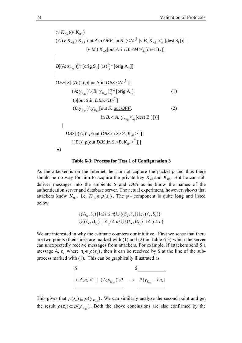
Validation of Protocols 74
1
2
1 2
1
2
z2 2
( )( )
( [( ) [out .in . in . (< > | , [dest S ])] |
( ) [out . in . < > [dest B ]]
|
[( ; z ) [orig S ].(; ) [orig A ]]
|
[ [ (
KBS AB
AB
AS BS
AB AS AB A
AB A
KK B B
v K v K
A v K K A OFF S A B K
v M K A B M
B A z
OFF S A
↑ < >
1 1
; ) .( [out .in .< > ] |
( ; ) .( ; y ) [orig A ]. (1)
( [out .in .< > ] | ( ;y ) .y [out . out .
KAS
AS AB
BS BS
yK K S
K K
p S DBS A
A y B
p S DBS BB S OFF
↑
↑
2 1
(2)
in . , y > [dest B ]]))]
|
[!( ; ) . [out .in .< , > ] |
!( ; ) . [out .in .< , > ]]]| )
ABK S
AS
BS
B A
DBS A p DBS S A K
B p DBS S B K
↑
↑
<
•
Table 6-3: Process for Test 1 of Configuration 3
As the attacker is on the Internet, he can not capture the packet p and thus there should be no way for him to acquire the private key ASK and BSK . But he can still deliver messages into the ambients S and DBS as he know the names of the authentication server and database server. The actual experiment, however, shows that attackers know BSK , i.e. ( )BSK zρ •∈ . The ϕ − component is quite long and listed below
2 2 1
1 2
{( , ) |1 } {( , )} {( , )}{( , ) |1 } {( , ) |1 }
i
j j
A i n S SB j n B j n• • •
• •
≤ ≤≤ ≤ ≤ ≤
∪ ∪∪ ∪
We are interested in why the estimate counters our intuitive. First we sense that there are two points (their lines are marked with (1) and (2) in Table 6-3) which the server can unexpectedly receive messages from attackers. For example, if attackers send S a message A, n• where ( )n zρ• •∈ , then it can be received by S at the line of the sub-process marked with (1). This can be graphically illustrated as
, | ( ; ) . { }
AS ASK K
S S
A n A y P P y n• •< > → →
This gives that ( ) ( )ASKz yρ ρ• ⊆ . We can similarly analyze the second point and get
the result ( ) ( )BSKz yρ ρ• ⊆ . Both the above conclusions are also confirmed by the

6.3 Protocol Validation in Hierarchical Networks 75
automated analysis. Attackers may also deliver messages to DBS. But they only cause DBS to send more packet p to S that in fact has no side-effect for authenticity. The analysis results, on the other hand, tell us that ( )
ABBS KK yρ∈ . Since this is the only way BSK can be sent onto the Internet, we can immediately sense that reconstructing how it happens is very important for identifying whether or not
( )BSK zρ •∈ is an over-estimate. After inspecting the possible values for the variables
ASKy and BSKy , we can simulate how analysis computes the estimate as below steps:
1. In the analysis the mailbox of DBS is initially
, | < ;
AS BS
DBS
A K B K< > >
by the over-approximation of the child-to-parent output from the packet p to the enclosing ambient DBS.
2. Suppose both
ASKy and BSKy are the name DBS which is given by attackers’
message. The continuous processes at the line (1) and (2) in Table 6-3 give the following structure of S and its evolvement
, | ( ; ) . , { }
,
AB AB
AS DBSK AS K BS
BS
S SDBS DBS
A KB y P A K P y K
B K
< >→ < > →
< >
This illustrates the reason for ( )ABBS KK yρ∈ . Please note that we are
simulating the computation of analysis: The ambient DBS constructed inside S is treated just as the same one outside S. Therefore their mailboxes are merged together.
As only DBS’ message contains the key BSK , we are sure that above steps is the only way used by analysis to achieve the estimate ( )
ABBS KK yρ∈ . 3. Now suppose
BSKy at the line (2) in Table 6-3 is any packet name known by attacker, i.e. p• , the continuous process gives an estimate of the ambient in the form

Validation of Protocols 76
out . out .in .
,
BS
OFFS
pS OFF B
A K
•
< >
As the figure shows, the mobility primitives will direct the packet to move onto the Internet. Then attackers can catch it and eventually get the key BSK as ( )p zρ• •∈ . Our assumption is possible even though in the second step we have chosen
BSKy to be DBS while now we assign BSKy the value p• . By reviewing the
scratch of the process
( ;y ) .y [...]BS BSK KB
we know that the analysis will attempt to simulate the creation of all ambients with the name that
BSKy may be bound to.
Summarizing the above steps, we are sure that the estimate ( )BSK zρ •∈ is an over-approximation given by the estimates of the first and third steps. Accordingly we can remove the pair 1( , )jB• for the ϕ − component since BSK is needed to decrypt message at the point of 1 jB .
But the other pairs are still useful and can be illustrated by the attacks listed below.
: , : [ , ]
: [ ]
A
BS
A
M S A KS B K A KM B K m
•
•
• •
→→→
: , [ , ] : [ , ] : ,
: [ , ] : [ ]
AS AB
BS AB
B AB
AB
A S A K B KS B K A KM S B KS M K A KA B K m
•
•
→→→→→
Attack 1 Attack 2
In attack 1, B finally believes that he is communicating with A although he is communicating with the attacker. The second attack makes use of the security hole at the line (2) in Table 6-3 by cheating S to send the attacker the key ABK and accordingly the attacker can read any message sent from A to B.
Test 2
In the first test we introduced the local network OFF and showed the keys ASK and
BSK are secure stored and retrieved. But there are still other security flaws existing in

6.3 Protocol Validation in Hierarchical Networks 77
the protocol. The root cause for these security issues is that the authentication server can not distinguish the packets from the database server with the packets from attackers. In this sub-section we try to fix the problem with a private key _S DBK only shared between the authentication server and the database server. Since now attackers can not cache packets communicated between the two servers which are both located in the office network, we do not have to worry about that the key may be explored by attackers.
The process is then declared in Table 6-4 on the next page and the major changes compared with the process in Table 6-3 are underlined.
1
2
1 2
1
2
z2 2
_
( )( )
( [( ) [out .in . in . (< > | , [dest S ])] |
( ) [out . in . < > [dest B ]]
|
[( ; z ) [orig S ].(; ) [orig A ]]
|( )
KBS AB
AB
AS BS
AB AS AB A
AB A
KK B B
S DB
v K v K
A v K K A OFF S A B K
v M K A B M
B A z
v K
↑ < >
_
1 1
_
2
1 1
2
[ [ ( ; ) .( [out .in .< > ] |
( ; ) [orig D ].( ; y ) [orig A ].
( [out .in .< > ] |
( ;y ) [orig D ].y [out . out . in
KS DB AS
AS AB
S DB
BS BS
yKK SD K S
KK SD K
OFF S A p S DBS A
A y B
p S DBS B
B S OFF
↑
↑
2
1
2
1
_ 1
_ 2
. , y > [dest B ]]))]
| [!( ; ) . [out .in .< , > [dest SD ]] |
!( ; ) . [out .in .< , > [dest SD ]]]]
| )
ABK S
S DB AS D
S DB BS D
B A
DBS A K DBS S A K
B K DBS S B K
<
•
Table 6-4: Process for Test 2 of Configuration 3
Comparing with the process in Table 6-3, we use the parent-child input instead of the local input in S and symmetrically replace the child-to-parent output with the local output in DBS. We also add labels to declare the crypto-points and authentication origins or intentions to compliant with the definition of the syntax.
The estimate of the process shows that there is no security flaw in the protocol.
Test 3
When there are thousands of keys managed by the database server, one can imagine that encrypting and decrypting every key required by the authentication server are very time-consuming. To fix this problem, we here suggest another way for the authentication server to determine whether or not a packet is from the database server.

Validation of Protocols 78
The idea is we use a unique number shared between the two servers but not known by others. This idea can be illustrated as:
1 1
1
1
1. : 1 . : {check }2. : , ,2 . : , , {check and }
AS
A A
A AS
u A K u A
S ADBS y y A
DBS u y KS x x x x u x A
→′ → =
→′ → = =
The first line describes that S asks the private key of A from DBS while line 1´ checks the ID of A. This time DBS replies the message including A’s ID and its private key together with the unique number 1u . By checking the unique number S ensures that the message is from DBS and believes the key received is not compromised. We can similarly apply the method for reading other keys stored on the authentication server. The process is then declared in Table 6-5 and the changes compared with the process in Table 6-3 are underlined.
1
2
1 2
1
2
z2 2
1
( )( )
( [( ) [out .in . in . (< > | , [dest S ])] |
( ) [out . in . < > [dest B ]]
|
[( ; z ) [orig S ].(; ) [orig A ]]
|( )(
KBS AB
AB
AS BS
AB AS AB A
AB A
KK B B
v K v K
A v K K A OFF S A B K
v m K A B m
B A z
v u v
↑ < >
1
2
2
1 1
2 1
)
[ [ ( ; ) .( [out .in .< > ] |
( , ; ) .( ; y ) [orig A ].
( [out .in .< > ] | ( , ;y ) .y [out . out . in . , y > [dest B ]]
KAS
AS AB
BS BS AB
yK K S
K K K S
u
OFF S A p S DBS A
u A y B
p S DBS Bu B S OFF B A
↑
↑
<
1
2
))]
|
[!( ; ) . [out .in .< , , > ] |
!( ; ) . [out .in .< , , > ]]]
| )
AS
BS
DBS A p DBS S u A K
B p DBS S u B K
↑
↑
•
Table 6-5: Process for Test 3 of Configuration 3
Our experiment result shows no authentication is violated in this solution and more important we do not encrypt or decrypt messages sent by DBS any more.
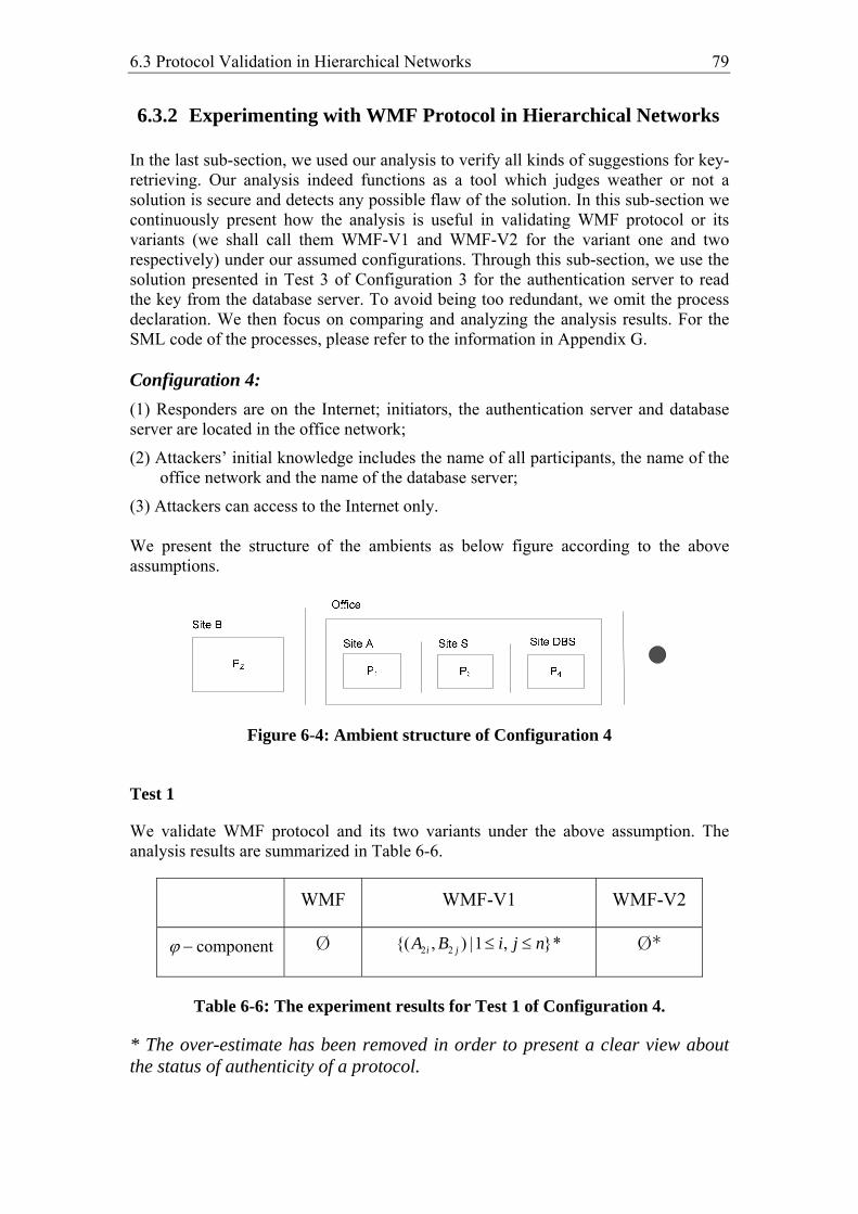
6.3 Protocol Validation in Hierarchical Networks 79
6.3.2 Experimenting with WMF Protocol in Hierarchical Networks
In the last sub-section, we used our analysis to verify all kinds of suggestions for key-retrieving. Our analysis indeed functions as a tool which judges weather or not a solution is secure and detects any possible flaw of the solution. In this sub-section we continuously present how the analysis is useful in validating WMF protocol or its variants (we shall call them WMF-V1 and WMF-V2 for the variant one and two respectively) under our assumed configurations. Through this sub-section, we use the solution presented in Test 3 of Configuration 3 for the authentication server to read the key from the database server. To avoid being too redundant, we omit the process declaration. We then focus on comparing and analyzing the analysis results. For the SML code of the processes, please refer to the information in Appendix G. Configuration 4: (1) Responders are on the Internet; initiators, the authentication server and database server are located in the office network;
(2) Attackers’ initial knowledge includes the name of all participants, the name of the office network and the name of the database server;
(3) Attackers can access to the Internet only. We present the structure of the ambients as below figure according to the above assumptions.
Figure 6-4: Ambient structure of Configuration 4
Test 1
We validate WMF protocol and its two variants under the above assumption. The analysis results are summarized in Table 6-6.
WMF WMF-V1 WMF-V2
ϕ − component Ø 2 2{( , ) |1 , }*i jA B i j n≤ ≤ Ø*
Table 6-6: The experiment results for Test 1 of Configuration 4.
* The over-estimate has been removed in order to present a clear view about the status of authenticity of a protocol.

Validation of Protocols 80
The results for WMF and WMF-V1 are just as those of the case that both initiators and responders are on the Internet. The change happens at the WMF-V2. It is flawless now. Here one implicit assumption is necessary to clarify that malicious legal sites belong to the class of attackers since they are malicious. These bad behavior sites could be initiators or responders. This concept is implicit in LySa as there is only one network and thus attackers and participants of a protocol stay on the same location. In a hierarchical network, however, we must be careful which site could be malicious. Take the above descriptions of the configuration for example, it actually forces the condition that every initiator is friendly; otherwise, attackers should be supposed to be in the office network and our assumption is violated. When we analyze the result for the WMF-V2, this implicit condition is applied to determine which pair(s) of the ϕ − component is(are) over-estimate.
Test 2
Observing that communication between A and S is transparent to attackers, we try to remove encryption of messages in the first step of WMF and extend the message with a unique number only known by S and A. The suggested protocol is described as:
1. : , , ,2. : [ , ]3. : [ ]
AB
BS AB
AB
A S u A B KS B K A KA B K M
→→→
There are three benefits given by the optimization: (1) This change saves the time for encrypting and decrypting the message in line 1; (2) It saves the space on the database server for storing the key ASK ; (3) It saves the time for the authentication server to get the key ASK from the database server. Even though we can expect that the protocol is secure, the actual experiment on our computer unfortunately can not afford the heavy computation and reported the error – “the RAM is used up”. This is because we have a four-tuple message (instead of three-tuple) that means the number of quantifications in ALFP formula is also increased. Suppose the number of the set of the universe U is n. Then increasing the number of quantification of a formula by one means the new computation time is up to n times as big as that of the former. Correspondingly, the space consumed by the solver is increased much too. Configuration 5: (1) Initiators are on the Internet; responders, the authentication server and database server are located in the office network;
(2) Attackers’ initial knowledge includes the name of all participants, the name of the office network and the name of the database server;
(3) Attackers can access to the Internet only.

6.3 Protocol Validation in Hierarchical Networks 81
We present the structure of the ambients as below figure according to the above assumptions.
Figure 6-5: Ambient structure of Configuration 5
Test 1
The analysis results are summarized in Table 6-7.
WMF WMF-V1 WMF-V2
ϕ − component Ø Ø* 2 2{( , ) |1 , }i jA B i j n≤ ≤ *
Table 6-7: The experiment results for Test 1 of Configuration 5.
* The over-estimate has been removed in order to present a clear view about the status of authenticity of a protocol.
Compared with the results in Table 6-6, the new results reflect the exchange of the locations of initiators and responders. As expected, now the communication between the server and responders are protected from the eavesdropping of attackers. Similar to the idea in the Test 2 of Configuration 4, we can remove the message encryption and decryption in the step 2.
1. : , [ , ]2. : , ,3. : [ ]
AS AB
AB
AB
A S A K B KS B u A KA B K M
→→→
The corresponding test shows that the optimized protocol is still secure with respect to authenticity.
Configuration 6: (1) Initiators are on the Internet; responders, the authentication server and database server are located in the office network; responders are movable and they may work on the Internet;
(2) Attackers’ initial knowledge includes the name of all participants, the name of the office network and the name of the database server;
(3) Attackers can access to the Internet only.

Validation of Protocols 82
We present the structure of the ambients as below figure according to the above assumptions.
Figure 6-6: Ambient structure of Configuration 6
Test 1
As no sites can move in our calculus, we normally need declare two separate processes: one is for the case that B is inside office network; another is for the case that B is on the Internet. After analyzing the two processes and removing the over-estimates in their ϕ − components individually, we unite the two ϕ − components. This will be treated as the estimate for the whole configuration. However, one can expect that the result will be the same as the case that the responders are on the Internet only (described by Configuration 3). If the protocol is flawed in the case that the responder is in the local network, then it also flawed when the responder is on the Internet as the attacker can get more information now. Our experiment on WMF and its two variants also confirmed our conjecture: for the three protocols the estimates based on this configuration are same with those based on Configuration 3. The analysis results for the two configurations are summarized in Table 6-8.
WMF WMF-V1 WMF-V2
ϕ − component Ø 2 2{( , ) |1 , }*i jA B i j n≤ ≤ 2 2{( , ) |1 , }i jA B i j n≤ ≤ *
Table 6-8: The experiment results for Test 1 of Configuration 6.
* The over-estimate has been removed in order to present a clear view about the status of authenticity of a protocol.
Configuration 7: (1) Initiators are on the Internet; responders, the authentication server and database server are located in the office network;
(2) Attackers’ initial knowledge includes the name of all participants, the name of the office network and the name of the database server;
(3) Attackers can access to the Internet and the office network. The structure of the ambients is specified as below figure according to the above assumptions.

6.4 Summary 83
Figure 6-7: Ambient structure of Configuration 7
Test 1
This time attackers acquired full capability to eavesdrop on any packet transferred between any two participants. We can reasonably guess that this configuration will have same estimates with the configuration described in Figure 6-2. The guess is proved by our experiment again: For all of the WMF, WMF-V1 and WMF-V2, attackers know all keys including ASK , BSK and ABK and thus the three protocols are completely cracked by the attacker.
Configuration 8: (1) Responders are on the Internet; initiators are in the office network; the authentication server and database server are located in the computation center;
(2) Attackers’ initial knowledge includes the name of all participants, the name of the office network, the name of the computation center and the name of the database server;
(3) Attackers can access to the Internet and the office network only. The structure of the ambients is specified as below figure
Figure 6-8: Ambient structure of Configuration 8
Test 1
The estimates for the three protocols are same as those in Table 6-8. As the two attackers share their knowledge each other, the effect of the boundary of the office network diminishes and thus in that sense site B can be thought to be on the Internet. This explains why we get the same result as the Test 1 of Configuration 6.
6.4 Summary
We have experimented on symmetric key protocols both in the flat space of networks and in hierarchical networks. Our estimate results show that our analysis works well

Validation of Protocols 84
for both of the two kinds of networks. In particular, our tool can safely approximate the behavior of the protocols which are applied on a hierarchical network. Some protocols are further optimized to improve their performance according to the specific network environment and assumptions. Our experience about the experiment can be summarized as below:
(1) As ambients can be used to formalize the objects which may be very different in properties considered in our model, such as local networks, data files, etc. one must be careful when locating the attacker to make sure the assumption is proper.
(2) The estimate computed by the analysis is an over-estimate. Therefore the skill of distinguishing between real answer and over-estimate is necessary. The two kinds of typical over-estimate in the analysis are illustrated in Test 1 of Configuration 3. As far as we know, they are the reason of all over-estimates found in our experiment.

85
7 Conclusion
In this chapter we summarize the key contributions and conclusions of this M.Sc. Thesis work that has been carried out in relation to the project “Static Analysis for Protocol Validation in Hierarchical Networks”. We end the chapter with the discussion of future work that could be performed to investigate interesting areas or lead to further clarifications or improvements on the existing work.
7.1 Overview of Contribution
The contribution of our work could be summarized as four aspects: The calculus. We have investigated how encryptions and decryptions could be expressed in ABoxed Ambients. This is important for deciding where to add annotations declaring the origin and destination of encrypted messages in order to check authentication property. We have also presented how hierarchical networks and protocols applied on such networks can be formalized as ABoxed Ambients processes. Participants of protocols and local networks are modeled as ambients. Packets are also modeled as ambients and their ability to move around is governed by the mobility primitives possessed. Since ambient calculus is very expressive, it sometimes attempts to assign the modeled objects more capabilities than what they are supposed to have, and thus some properties of the object are changed or vanished. To describe the characteristic of objects more precisely, we remove the undesired capabilities from these objects. This was achieved by our well-formednesses which classify the ambients into the ambients of sites and the ambients of packets. Static analysis. The static analysis has been developed for tracking the set of encrypted messages decrypted at each relevant point successfully. Since the notion of authentication is directly captured by the operational semantics, it can also be safely estimated by the analysis. We have also proved the correctness of the analysis with respect to the operational semantics in order to ensure that the analysis can safely estimate the behavior of a process throughout its execution. Network attacker. Our attacker is based on the classic Dolev-Yao attacker. Moreover we have added necessary assumptions onto the Dolev-Yao condition to complaint with the environment of the hierarchical network. We then defined the adjusted Dolev-Yao condition. Last we have proved that the attacker is hardest with respect to the well-formednesses. Other kinds of attackers that may be modeled by ambient calculus have also been discussed. The implementation and experiments on protocols. Following the implementation of the analysis, we have developed a tool in SML of New Jersey to automate our analysis. With the help of the tool, we validated many symmetric key protocols which are formalized as ABoxed Ambients processes. Our experiment results have shown that the analysis can pinpoint many kinds of errors that can be captured by LySa in the environment of hierarchical networks.

Conclusion 86
7.2 Future Work
Several areas or solutions have been examined in thought but have not been put into practice for the restriction on time. They are listed as below. • Extending the calculus with asymmetric keys.
Our framework can be adapted to deal with perfect asymmetric cryptography as demonstrated in [2, chapter 8]. The idea can be sketched as follows. First we define the set of names for pairs of asymmetric keys m+ and m− :
:: site name | non-site name
| non-site name
| non-site name
s s s
P
P
P
C n nn n
m m
m m
+
−
= ∈∈
∈
∈
CC
C
C
The process P has two more constructs for creating a new pair of public/private keys.
::... | ( ) key pair creation | ( ) key pair creation which is transparent to the attacker
P
v m Pvk m P
=
±±
We shall say that ⎣ ⎦m , m+⎢ ⎥⎣ ⎦ , m−⎢ ⎥⎣ ⎦ are pairwise distinct. Surely we need modify the rules for substitution and add more rules for congruence like LySa does. In particular, we add three additional reduction rules
1
1 1 1
(A-New) (A-News)
( ) ( ) ( ) ( )
( Output-Par2)
( , , , )( , , ; , , ) [orig ]. | [ , , [dest
ji i im
j j k k
P Q P Qv m P v m Q vk m P vk m Q
A
M MM M x x P m M M
+=
−′+
→ →± → ± ± → ±
−
′ ′ ′∧ = ∧′ ′ ′⋅ ⋅ ⋅ ⋅⋅ ⋅ < ⋅⋅⋅ >
R R
R R
R L LL
1 1
1
1 1 1
] | ]
{ } { } | [ ]
( Output-Par3)
( , , , )( , , ; , , ) [orig ]. | [ , ,
k k
ji i im
j j k k
R
P x M x M n R
A
M MM M x x P m M M
−=
+′+
→
← ⋅⋅⋅ ←
−
′ ′ ′∧ = ∧′ ′ ′⋅ ⋅ ⋅ ⋅⋅ ⋅ < ⋅⋅⋅
RL
R L LL
1 1
[dest ] | ]
{ } { } | [ ]k k
R
P x M x M n R
> →
← ⋅⋅⋅ ←RL
Accordingly we can extend our analysis, attacker and implementation to subject to the changes in the calculus. Certainly the theorems or lemmas relating to the changes should be modified or extended too.

7.2 Future Work 87
• Optimizing the Flow Logic specification to improve the performance of the Succinct Solver.
The actual formulation of the analysis has a great impact on the execution time on the solver. Two strategies are suggested in [34] to fasten the computation of the Succinct Solver. They are
(1) Adjusting the order of the parameters of relations.
The Succinct Solver uses prefix trees as an internal representation of relations [13]. Therefore, a generic strategy is to try to put the bound parameters ahead of the unbound ones. For example, assume that a relation 1 2( , )x xγ is a precondition in which 1x is always unbound but 2x is always bound. Then querying the inverse relation 2 1( , )x xγ ′ would be faster than querying 1 2( , )x xγ .
(2) Adjusting the order of conjunctions in preconditions.
Preconditions of an ALFP formula are evaluated from left to right. During the evaluation the environment which records the successful bindings of variables are kept updating. When checking a query to a relation γ , the evaluation of the remaining preconditions is performed under the updated environment that is calculated by unifying the current environment with the elements in γ . If the unification fails, then no further evaluation is needed. That is the earlier a unification fails, the less effort is in environment updating. Therefore we should arrange the query, which restricts the variable binding most, ahead of other preconditions. For example, for the clause
, : ( , ) ( )x y x y Site xγ∀ ∀ ∧ ⇒ ⋅⋅⋅
if x may be bound with more values in relation γ than those in relation Site, then reordering the preconditions as
, : ( ) ( , )x y Site x x yγ∀ ∀ ∧ ⇒ ⋅⋅⋅
is more efficient. As we have one incomplete experiment whose computation is too large to be afforded by our computer, we expect the optimizations of the specification can reduce the size of computation and complete the experiment. • Defining other attackers Our attacker is basic among the attackers could be modeled by the ambient calculus. Although we discussed three more powerful attackers in Chapter 4, what security property these attackers may be useful to validate need further investigation. Still more other attackers not listed in this thesis may exist and are waiting for us to explore.

88
Appendix A Protocol Narrations
Wide Mouthed Frog. [31]
1. : , [ , ]2. : [ , ]3. : [ ]
AS AB
BS AB
AB
A S A K B KS B K A KA B K M
→→→
The initiator’s name is not encrypted: 2. : , [ ]BS ABS B A K K→ The responder’s name is not encrypted: 1. : , , [ ]AS ABA S A B K K→ NeedHam-Schroeder (symmetric key). [30]
1. : , , 2. : [ , , , [ , ]]3. : [ , ]4. : [ ]5. : [ 1]6. : [ ]
A
AS A AB BS AB
BS AB
AB B
AB B
AB
A S A B RS A K R B K K A KA B K A KB A K RA B K RA B K M
→→→
→→ −→
Correcting the flaw
1
2
4. : [ , ]5. : [ , 1]
AB B
AB B
B A K u RA B K u R→→ −
Otway-Rees. [27]
1. : , [ , , , ]2. : , [ , , , ], [ , , , ]3. : , [ , ], [ , ]4. : , [ , ]5. : [ ]
AS A
AS A BS B
AS A AB BS B AB
AS A AB
AB
A B N K N N A BB S N K N N A B K N N A BS B N K N K K N KB A N K N KA B K M
→→→→
→
Yahalom. [29]
1. : ,2. : , [ , , ]3. : [ , , , ], [ , ]4. : [ , ], [ ]5. : [ ]
A
BS A B
AS AB A B BS AB
BS AB AB B
AB
A B A NB S B K A N NS A K B K N N K A KA B K A K K NA B K M
→→→→
→
Andrew Secure RPC. [28]

89
1. : , [ ]2. : [ 1, ]3. : [ 1]4. : [ , ]5. : [ ]
AB A
AB A B
AB B
AB AB B
AB
A B A K NB A K N NA B K NB A K K NA B K M
→→ +→ +
′ ′→′→
Correcting the flaw:
1
2
3
4
1. : , [ , ]2. : [ , 1, ]3. : [ , 1]4. : [ , , ]
AB A
AB A B
AB B
AB AB B
A B A K u NB A K u N NA B K u NB A K u K N
→→ +→ +
′ ′→

90
Appendix B Validation of Other Protocols
B.1 Validating Otway-Rees.
The extended protocol narration of Otway-Rees is specified as
1
1
1 2
1. : , [ , , , ][dest S] {assuming , are new values} : ,2. : , , [ , , , ][dest S] {assuming is new value} : , , [
AS A A
N
N BS B N B
N AS A
A N K N N A B N NB z z
B z z K N z A B NS y y y K N
→→
→→
1
2
, , , ], [ , , , ] : decrypt as [ , , , ][orig A] {check , and }
decrypt as [ , , , ][orig B] {check ,A
B
BS B
AS N N A B N N A B
BS N N A B N N
N A B K N N A BS y K y y y y y y y A y B
y K y y y y y y
′ ′= = =
′′ ′ ′ ′′ ′=
2 3
3
and }
3. : , [ , ][dest A], [ , ][dest B] {assuming is new value}
: , , {check } : decrypt as [ , ][ori
A B
B AB
A B
N AS N AB BS N AB AB
N N N
BS N K
y A y B
S y K y K K y K K
B z z z z zB z K z z
′ ′= =
→
′ ′→ =
2
1
1
g S] {check }
4. : , : , {check } : decrypt as [ , ][orig S] {check }
5. : [ ][dest B] {assum
B
A AB A
AB
N B
N
N N
AS N K N A
K
z N
B z zA x x x NB x K x x x N
A x M
=
→→ =
=
→
4
4
ing is a new value}
: : decrypt as [ ][orig A]
ABK M
M
B zB z z z
→
The ABoxed Ambients specification of the protocol is accordingly declared as
1
2
3
1
4
3
( )( )
( [( ) ( ) ( [out . in . ( | out B.in S.( | , , , [dest S ]))] |
( ;) .( ; ) [orig S ].
( ) [out . in . < > [dest B ]] )]
|[(; )
AS
AB
AB
AS BS
A AS A A
KA K A
K A
N
v K v K
A v N v N K A B N N A B N N
N N x
v M x A B M
S y
↑ ↑< > < > < >
1 2
3
4
1 1
2
2
. ( , , ; ) [orig A ].( , , ; ) [orig B ].( )
[out . in . ( | , [dest B ] |
[out .out .in .( | . [dest A ]])]]]
|
AS BS
A B
B
A
K KN N S N N S AB
BS N N AB S
AS BS N N AB S
A B y y A B y y v K
K S B y y K
K K B A y y K
B
↑
↑
< > < >
< > < >
1
2 3
2
3 3
[(; ) .( )( [out . in . , , , [dest S ]] |
(; ) .( ; ) [orig S ].(; ) [orig A ]. )])
|
KBS AB
AB
N B BS N B B
zKN B K B M B M
z v N K B S A B z N
z N z z z
< >
⋅⋅⋅ ⋅ ⋅⋅
•

91
The experiment result shows there is no authentication violation in Otwee-Rees as expected. But a phenomenon caused our attention: The computing time of the analysis for the protocol is apparently longer than the one of WMF and Needham-Schroeder. By analyzing the result of Otwee-Rees we found a large number of four-tuple messages and it is believed that the most of them are created by A_DY
RMF attackers. Thus we conclude that the longer the arity is, the more messages attackers can make.
B.2 Validating Yahalom.
The extended protocol narration of Yahalom is specified as
1
1. : , {assuming is a new value}
: , {assuming }
2. : , [ , , ][dest S] {assuming is a new value}
: , {check
A
A
A A
A N A
BS A N B B
B
A A N N
B z z z A
B B K z z N N
S y y y
→
→ =
→
→
1
1 2
}
: decrypt as [ , , ][orig B] {check }
3. : [ , , , ][dest A], [ , ][dest B] {assuming is a new value}
: ,
:
A B
A B
B
BS A N N A
AS B AB N N BS A AB AB
B
S y K y y y y A
S K y K y y K y K K
A x x
A
=
=
→
→
1
2
1 2
1
decrypt as [ , , , ][orig S] {check }
4. : , [ ][dest B]
: ,
: decrypt as [ , ][orig S] {check }
decry
AB A B
AB B
AB
AS B K N N B
K N
BS A K A
x K x x x x x B
A x x x
B z z
B z K z z z A
=
→
→
=
2
3
3
pt as [ ][orig A]
5. : [ ][dest B] {assuming is a new value}
:
: decrypt as [ ][orig A]
B
AB
AB
AB N
K
K M
z K z
A x M M
B z
B z z z
→
→
Based on the above extended protocol narration, we program the protocol below.

92
1 2
2 3
2 3
2 3
( )( )
( [( ) [out . in . , ] |
( , ; , ) [orig S ]. [out . in . [dest B ]]
( ) [orig B ]. [out A. in B. [dest B ]] |
AS
AB B AB B
KAB
B AB B
AS BS
A AK
A K N A K N A
xR A K N A
v K v K
A v N p A B A N
B N x x x A B x
x x x
↑< >
< >
< >
4
1
2
4
1
2
( ) [out . in . < > [dest B ]] )]
|[( ; ) .( ; , ) [dest B ]( )
[out . in . ( , , , [dest A ] |
[out .out .in . , >
AB
BS
A B
A B
K A
KN N S AB
AS N AB N S
BS AS AB
v M x A B M
S B A y y v K
K S A B y K y
K K A B A K
< >
<3
1
2 3 4
2
1
3 3 4
[dest B ]])]]
|
[( ; ) .( ) [out . in .( | , , [dest S ])] |
( ; ) [orig S ].( ;) [orig A ].(;z ) [orig A ]. ])
|
A A
K KBS AB AB
AB
S
N B BS N B B
z zKK B B B M B M
B A z v N K B S B A z N
A z N z
↑< > < >
⋅⋅⋅ ⋅ ⋅⋅
• The ϕ − component of the estimate reports a pair which is actually an over-estimation.
B.3 Validating Andrew Secure RPC.
We expand the protocol narration for Andrew Secure RPC as
1
1
1. : , [ ][dest B] {assuming is a new value} : , {check } : decrypt y as [ ][orig A]
2. : [ 1, ][dest A] {assuming is a nA
A
AB A A
A A
AB N
AB N B B
A A K N NB y y y AB K y
B K y N N
→→ =
→ +
1
1 1 1
2
2 1
ew value}
: : decrypt as [ , ][orig B] {check 1}
3. : [ 1][dest B]
: : decrypt y as [ ][orig A] {check
A B A
B
B
AB N N N A
AB N
AB N
A xA x K x x x N
A K x
B yB K y y
+ +
+
→= +
→ +
→
1
2
2
5. : [ ][dest B] {assuming is
1}
4. : [ , ][dest A] {assuming and are new values} : : decrypt as [ , ]
AB
B
AB B
K
N B
AB AB B AB B
AB K N
A x M M
N
B K K N K NA xA x K x x
′
+
′ ′
→
= +
′ ′ ′ ′→→
3
3
a new value}
:
: decrypt as [ ][orig A]ABK M
B y
B y z z
→

93
The corresponding specification in ABoxed Ambients is coded as
1
2 3
4
1
2 3
4
( )
( [( ) [out . in . ( | [dest B ])] |
( , ; ) [orig B ]. [out . in . , [dest B ])] |
(; , ) [orig B ]. ( ) [out . in
AB
B B B
AB
AB B AB
AB
A AB A A
KA A N A AB N N A
KK N A K
v K
A v N K A B A N
N N x K A B x x
x x v M x A
↑
′ ′ ′
< > < >
< >
5
1 2
3 4
5
1 2
3 4
. < > [dest B ]] )]
|[( ; ) .(; ) [orig A ].( ) ( [out . in . , , [dest A ] ]|
( ,N ;) [orig A ].( )( ) ( [out . in . , [dest A ] ]|
AB
A A A
AB
A
KN B B AB N N B B
KB B B AB B AB AB B B
B M
B A y v N K B A y y N
N v K v N K B A K N
< >
′ ′ ′ ′< >
5 5 (; ) [orig A ]. ))])
|
ABKM B My y′ ⋅ ⋅ ⋅ ⋅ ⋅⋅
•
Similar to Needham-schroeder, Andrew Secure RPC has successor operation. And the operation is encoded by the pair of a number. The estimate is summarized as
3 4{( , ) |1 }i iA A i n≤ ≤
Correcting the flaw The problem is quite similar to the flaw reported for Needham-schroeder. The way for fixing the flaw, therefore, is also similar: Add extra components 1 2( , , )u u ⋅ ⋅ ⋅ in the encrypted messages. The extended narration for the corrected steps is presented below.
1 1
1
1
1 1
2
1. : , [ , ][dest B] {assuming is a new value} : , {check } : decrypt y as [ , ][orig A] {check }
2. : [ , 1, ][A
A
AB A A
A A
AB u N u
AB N B
A A K u N NB y y y AB K y y y u
B K u y N
→→ =
=
→ +
2 2
1
1 1 2 1
3
2
dest A] {assuming is a new value}
: : decrypt as [ , , ][orig B] {check and 1}
3. : [ , 1][dest B]
:
A B A
B
B
AB u N N u N A
AB N
N
A xA x K x x x x u x N
A K u x
B yB
+ +
→= = +
→ +
→
3 32 1 3 1
4
2
2
: decrypt y as [ , ][orig A] {check and 1}
4. : [ , , ][dest A] {assuming and are new values} : : decrypt as [
B BAB u N u N B
AB AB B AB B
AB u
K y y y u y N
B K u K N K NA xA x K x
+ += = +
′ ′ ′ ′→→
4 4 4, , ] {check }AB BK N ux x x u′ ′ =
The experiment on the modified protocol shows the static authentication success. This should also guarantee the dynamic authentication.

94
Appendix C Generation Function of the Attacker
The generation function G(• , ∗ ) is written in ALFP logic as the conjunction ∧ of below formulae.
+k
+k
+k
1 1 1
1 1
1
1 1
1.1 ,..., : ( , ,..., , , ) genCap( )
1.2 , ,..., , , : ( , ) Pack( ) ( , ,..., , , )
( , , ,..., , , )2 , ,..., , , : ( , , ,...
kk k i ik A
k c k ck A
k c
k ck A
v v v v AW v
v v l v v l
t v v lv v l t v
κ ε
µ γ µ µ κ µ
ρ µµ ρ µ
=∈
∈
•
•∈
∧ ∀ ∗ ⇒ ∧
∧ ∀ ∗ ∧ ∧
⇒∧ ∀
+k
+k
1
1 1
1
1 1
, , , ) ( , )
( , ) (( AW) ( , ))
3.1 ,..., , : ( , ) ( , ) ( ) ( ) Pack( )
( , , ,..., , ,AW)
3.2 ,..., , : ( ,
k c
ki i c
kk i ik A
kk
k ik A
v l z
z v l
v v z v z in m out m
t v v
v v z v
ρ µ
ρ ϕ
µ ρ ρ µ µ µ µ
ρ µ
µ ρ
•
= • •
= • •∈
• •
= •∈
∧ ⇒
∧ ∧ ≠ ⇒
∧ ∀ ∧ ∧ ∧ ≠ ∧ ≠ ∧
⇒
∧ ∀ ∧
+k
1
1 1 1
) Reach( , )
( , , ,..., , ,AW)4.1.1 , : ( , ) in( ) out( ) Pack( ) : Reach( , ) ( , )4.2 , ,..., , , : ( , , ,..., , , ) ( , ,..., , , )
5.1
i
k
k c k c k ck A
t v vt m z t t m t m t
tv v l t v v l v v l
µ
ρ µ ερ µ µ
γ µµ ρ µ κ µ
•
•
•∈
∧ ∗
⇒
∀ ∧ ≠ ∧ ≠ ∧ ∧∀ ∗⇒∧ ∀ ⇒
f v
f
v
( , ) ( , ) ( : ( ) ( , )) ( : ( ) ( , ))5.2 ( , in( )) ( ,out( )) ( : ( ) ( ,in( )) ( ,out( )))
( : ( ) ( ,in( )) ( ,out( )))
z n z n t t z t t t z tz n z nt t z t z t
t t z t z t
ρ ρ ρ ρρ ρ
ρ ρ
ρ ρ
∗• • • • •
• • • •
• •
∗• •
∧ ∧ ∀ ⇒ ∧ ∀ ⇒
∧∀ ⇒ ∧ ∧
∀ ⇒ ∧
★ N N
N
N
The auxiliary function Reach and genCap are transformed as the conjunction of the below formulae.
Formulae for Reach Formulae for genCap
1 2 1 2
1 2 1 2
1 2
1 2 1 2
1 2
2 1
1 2 3 1 2 2
1 :Site( ) Reach( , )2 , :Site( ) Site( ) ( , ) ( , ) ( , ) Reach( , )3 , :Site( ) Site( ) Reach( , ) Reach( , )4 , , : Reach( , ) Reach( ,
z z
µ µ µ µµ µ µ µρ µ ρ µ γ µ µ
µ µµ µ µ µ
µ µµ µ
µ µ µ µ µ µ µ
• •
∀ ⇒∀ ∧ ∧
∧ ∧⇒∀ ∧ ∧
⇒∀ ∧ 3
1 3
) Reach( , )µ µ⇒
1 : in( ) ( ,out( )) ( , )2 : out( ) ( ,in( )) ( , )3 : in( ) out( ) ( ,out( )) ( ,in( ))
i
i
i i
i i
t v tz t z t
t v tz t z t
t v t v tz v z v
ρ ρ
ρ ρ
ρ ρ
• •
• •
• •
∀ =⇒ ∧∀ =
⇒ ∧∀ ≠ ∧ ≠
⇒ ∧

95
Appendix D Proofs
D.1 Correctness of the Analysis
Theorem 1: Subject reduction If P → QR and ( , , ) :Pγ κ ρ ϕ∗ then ( , , ) :γ κ ρ ϕ∗ Q . Proof. We prove the more general result
If P → QR and ( , , ) :Pγ κ ρ ϕ∗ then ( , , ) :γ κ ρ ϕ∗ Q ; furthermore, if ϕ = Ø then RMP → Q .
The proof proceeds by structural induction in the reduction steps. Case (New). Assume that ( , , ) ( ) :v n Pγ κ ρ ϕ∗ i.e. that ( , , ) :Pγ κ ρ ϕ∗ . Assume also that ( ) ( )v n P v n P′→ using (New) because P P′→ . Then by the induction hypothesis ( , , ) :Pγ κ ρ ϕ∗ ′ , which by the analysis definition allows to conclude ( , , ) ( ) :v n Pγ κ ρ ϕ∗ ′ . Case (News) is similar to the case (New). Case (Amb). Assume that ( , , ) [ ] :n Pγ κ ρ ϕ∗ i.e. that ( ) : ( ) ( , ,nρµ µ γ γ κ∀ ∈ ∈ ∗ ∧N
) :Pµρ ϕ . As ( )nρN is { n⎢ ⎥⎣ ⎦ }, we can write the formula equivalently to be
( ) ( , , ) :nn Pγ γ κ ρ ϕ⎢ ⎥⎣ ⎦∈ ∗ ∧⎢ ⎥⎣ ⎦ (where n is its canonical version). We further assume that [ ] [ ]n P n P′→ by (Amb) because P P′→ . Then by the induction hypothesis ( , , ) :n Pγ κ ρ ϕ⎢ ⎥⎣ ⎦ ′ , which together with ( )n γ∈ ∗⎢ ⎥⎣ ⎦ and ( ) nnρ = ⎢ ⎥⎣ ⎦N allows to
conclude ( , , ) [ ] :n Pγ κ ρ ϕ∗ ′ by the analysis definition. Case (Par). Assume that 1 2( , , ) | :P Pγ κ ρ ϕ∗ i.e. that 1( , , ) :Pγ κ ρ ϕ∗ and
2( , , ) :Pγ κ ρ ϕ∗ . Furthermore, assume that 1 2 1 2| |P P P P′→ by (Par) because P P′→ . The applying the induction hypothesis ( , , ) :Pγ κ ρ ϕ∗ ′ . The analysis allows to conclude that 1 2( , , ) | :P Pγ κ ρ ϕ∗ ′ . Case (Congr) is directly given by the induction hypothesis and Lemma 2. Case (In). Let 1 2[in . | ] | [ ]P m n P n P= Q and 1 2[ [ | ] ]P n m P P′ = Q | where pm∈C and
assume that ( , , ) :Pγ κ ρ ϕ∗ and that P P′→ due to (In). We have to prove ( , , ) :Pγ κ ρ ϕ∗ ′ . Expanding the analysis, we get

96
1 2
1
2
( , , ) :
iff ( , , ) [in . | ] : ( , , ) [ ] :
iff ( ) : ( ) ( , , ) in . | :
( , , ) [ ] :
iff ( ) : ( ) (in ) ( ) ( , , )
P
m n P n P
m n P
n P
m n
µρ
ρ ρ
γ κ ρ ϕ
γ κ ρ ϕ γ κ ρ ϕ
µ µ γ γ κ ρ ϕ
γ κ ρ ϕ
µ µ γ γ µ γ κ ρ
∗
∗ ∗
∗
∧
∀ ∈ ∈ ∗ ∧ ∧
∧
∀ ∈ ∈ ∗ ∧ ⊆ ∧
N
N M
Q
Q
1
in 2
1
in
2
| :
in (in ) : ( ) ( , , ) [ ] :
iff ( ) : ( ) (in ) ( ) ( , , ) | : in (in ) : ( )
( ) : ( ) ( , , ) :
P
n n P
m n Pn
n P
µ
ρ
µρ ρ
ρ
µρ
ϕ
µ ϕ µ γ κ ρ ϕ
µ µ γ γ µ γ κ ρ ϕ
µ ϕ µ
µ µ γ γ κ ρ ϕ
∗
′′
∧
′ ′∧∀ ∈ ∧
∀ ∈ ∈ ∗ ∧ ⊆ ∧ ∧
′ ′∧∀ ∈ ∧
′′ ′′∀ ∈ ∈ ∗ ∧
M
N M
M
N
Q
Q
The inϕ closure condition gives at least one more constraint ( )m nγ∈⎢ ⎥ ⎢ ⎥⎣ ⎦ ⎣ ⎦ . Since by ( ) { }nnρ = ⎢ ⎥⎣ ⎦N , ( ) { }mmρ = ⎢ ⎥⎣ ⎦N and (in ) {in }nnρ = ⎢ ⎥⎣ ⎦M , we equivalently rewritten
the above analysis as
in
1
2
( ) (in ) ( ) ( )
( ) ( , , ) | :
( ) ( , , ) :
m
n
m n m m
m n
n
P
P
γ γ ϕ
γ γ κ ρ ϕ
γ γ κ ρ ϕ
⎢ ⎥⎣ ⎦
⎢ ⎥⎣ ⎦
∈ ∗ ∧ ⊆ ∧ ∧⎢ ⎥ ⎢ ⎥ ⎢ ⎥ ⎢ ⎥⎣ ⎦ ⎣ ⎦ ⎣ ⎦ ⎣ ⎦
∈ ∧ ∧⎢ ⎥ ⎢ ⎥⎣ ⎦ ⎣ ⎦
∈ ∗ ∧⎢ ⎥⎣ ⎦
Q (1)
By the analysis of the ambient and the fact ( ) { }mmρ = ⎢ ⎥⎣ ⎦N , we have
1
1
1
( ) ( , , ) | :
iff ( ) : ( ) ( , , ) | :
iff ( , , ) [ | ] :
m
n
m n
n
P
m P
m P
µρ
γ γ κ ρ ϕ
µ µ γ γ κ ρ ϕ
γ κ ρ ϕ
⎢ ⎥⎣ ⎦∈ ∧⎢ ⎥ ⎢ ⎥⎣ ⎦ ⎣ ⎦∀ ∈ ∈ ∧⎢ ⎥⎣ ⎦N
Q
Q
Q
(2)
The analysis of the parallelism then gives
1 2
1 2
( , , ) [ | ] : ( , , ) :
iff ( , , ) [ | ]| :
n n
n
m P P
m P P
γ κ ρ ϕ γ κ ρ ϕ
γ κ ρ ϕ
⎢ ⎥ ⎢ ⎥⎣ ⎦ ⎣ ⎦
⎢ ⎥⎣ ⎦
∧Q
Q (3)
By the analysis of the ambient and the fact ( ) { }nnρ = ⎢ ⎥⎣ ⎦N , we have
1 2
1 2
1 2
( ) ( , , ) [ | ]| :
iff ( ) : ( ) ( , , ) [ | ]| :
iff ( , , ) [ [ | ]| ] :
nn m P P
n m P P
n m P P
µρ
γ γ κ ρ ϕ
µ µ γ γ κ ρ ϕ
γ κ ρ ϕ
⎢ ⎥⎣ ⎦
∗
∈ ∗ ∧⎢ ⎥⎣ ⎦∀ ∈ ∈ ∗ ∧N
Q
Q
Q
(4)
Applying (2), (3) and (4) on (1) sequentially, we finally get
in
1 2
( ) (in ) ( ) ( )
( , , ) [ [ | ]| ] :
m n m m
n m P P
γ γ ϕ
γ κ ρ ϕ∗
∈ ∗ ∧ ⊆ ∧ ∧⎢ ⎥ ⎢ ⎥ ⎢ ⎥ ⎢ ⎥⎣ ⎦ ⎣ ⎦ ⎣ ⎦ ⎣ ⎦Q
It then gives 1 2 ( , , ) [ [ | ]| ] :n m P Pγ κ ρ ϕ∗ Q i.e. that ( , , ) :Pγ κ ρ ϕ∗ ′ as required. Case (Out) is similar to the case (In).

97
Case (LocCom). Let 1 k 1 1 1M , , M [dest ] | ( , , ; , , ) .j j kP M M x x P+′ ′=< ⋅⋅⋅ > ⋅⋅⋅ ⋅ ⋅ ⋅L and
1 1 1{ } { }k kP P x M x M′ = ← ⋅⋅⋅ ← and assume that ( , , ) :Pγ κ ρ ϕ∗ and that P P′→ because of (LocCom). We have to prove ( , , ) :Pγ κ ρ ϕ∗ ′ . Unfolding the analysis one gets
1 1 1
1 1 1
1
( , , ) :
iff ( , , ) , , [dest ] : ( , , ) ( , , ; , , ) . :
iff , , : ( ) < , , [dest ] ( ) (1)
< , ,
k j j k
kk i i i k
k
P
M M M M x x P
v v v M v v
v vρ
γ κ ρ ϕ
γ κ ρ ϕ γ κ ρ ϕ
κ
∗
∗ ∗+
=
′ ′< ⋅⋅⋅ > ∧ ⋅⋅⋅ ⋅ ⋅ ⋅
∀ ⋅⋅⋅ ∧ ∈ ⇒ ⋅⋅⋅ > ∈ ∗ ∧
⋅⋅⋅ >
L
M L
1
1
[dest ] ( ): ( ) (2)
( ) i
ji i i
ki j i x
v M
vρκ
ρ=
= +
′∈ ∗ ∧ ∈
⇒ ∧ ∈ ∧⎢ ⎥⎣ ⎦
L M
*1
(3)
( RM( , , , ) ( , ) ) ( , , ) : (4)Pε ε ϕ γ κ ρ ϕ¬ ⇒ ∈ ∧D L
Since fv( iM ) = Ø then (1) gives 1 , , [dest ] ( )kM M κ< ⋅⋅⋅ > ∈ ∗⎢ ⎥ ⎢ ⎥⎣ ⎦ ⎣ ⎦ L . The assumption
1 ji i iM M= ′∧ = then gives 1 ( )i
ji iM Mρ= ′∧ ∈⎢ ⎥⎣ ⎦ M . Now from (3) and (4) we get
1 ( )i i
ki j M xρ= +∧ ∈⎢ ⎥ ⎢ ⎥⎣ ⎦ ⎣ ⎦ and *( , , )γ κ ρ 1:P ϕ . The Lemma 1 then gives
*1 1 1( , , ) { } { }:k kP x M x Mγ κ ρ ϕ← ⋅⋅⋅ ← i.e. that ( , , ) :Pγ κ ρ ϕ∗ ′ as required. For the
second part of the result we see that RM( , , , ) ( , )ε ε ϕ¬ ⇒ ∈D L follows from (2) and since ϕ = Ø it must be the case that RM( , , , )εD L . Therefore the conditions of the rule (LocCom) are met for RM→ . Case (Output-Chd1). Let 1 k 1 1 1M , , M | [( , , ; , , ) . | ]n
j j kP n M M x x P+′ ′=< ⋅⋅⋅ > ⋅⋅⋅ ⋅ ⋅ ⋅ Q and
1 1 1[ { } { }| ]k kP n P x M x M′ = ← ⋅⋅⋅ ← Q and assume that ( , , ) :Pγ κ ρ ϕ∗ and that P P′→ because of (Output-Chd1). We have to prove ( , , ) :Pγ κ ρ ϕ∗ ′ . Expanding the analysis one gets
1 1 1 1
1 1
1
( , , ) :
iff ( , , ) , , : ( , , ) [( , , ; , , ) . | ] :
iff ( ( ) : (*)
, , : ( )
< , , [dest ] ( ))
( , , ) [(
nk j j k
kk i i i
k
P
M M n M M x x P
n
v v v M
v v
n
ρ
ρ
ε
γ κ ρ ϕ
γ κ ρ ϕ γ κ ρ ϕ
µ µ γ
κ µ
γ κ ρ
∗
∗ ∗+
=
∗
′ ′< ⋅⋅⋅ > ∧ ⋅⋅⋅ ⋅ ⋅ ⋅
∀ ∈ ∈ ∧
∀ ⋅⋅⋅ ∧ ∈
⇒ ⋅⋅⋅ > ⊆ ∧
N
M
D
Q
1 1 1
1 1
1
1 1 1
, , ; , , ) . | ] :
iff ( ( ) : (*)
, , : ( )
< , , [dest ] ( ))
( ) : ( ) ( , , ) ( , , ; , , ) . | :
j j k
kk i i i
k
j j k
M M x x P
n
v v v M
v v
n M M x x P
ρ
ρ
ε
µρ
ϕ
µ µ γ
κ µ
µ µ γ γ κ ρ ϕ
+
=
′+
′ ′⋅ ⋅ ⋅ ⋅ ⋅ ⋅
∀ ∈ ∈ ∧
∀ ⋅⋅⋅ ∧ ∈
⇒ ⋅⋅⋅ > ⊆ ∧
′ ′ ′ ′∀ ∈ ∈ ∗ ∧ ⋅⋅⋅ ⋅⋅ ⋅
N
M
D
N
Q
Q

98
1 1
1
1 1 1
iff ( ( ) : (*)
, , : ( )
< , , [dest ] ( ))
( ) : ( ) ( , , ) ( , , ; , , ) . ( , , ) :
iff ( ( ) : (*)
kk i i i
k
j j k
n
v v v M
v v
n M M x x P
n
ρ
ρ
ε
µ µρ
ρ
µ µ γ
κ µ
µ µ γ γ κ ρ γ κ ρ ϕ
µ µ γ
=
′ ′+
∀ ∈ ∈ ∧
∀ ⋅⋅⋅ ∧ ∈
⇒ ⋅⋅⋅ > ⊆ ∧
′ ′ ′ ′∀ ∈ ∈ ∗ ∧ ⋅⋅⋅ ⋅⋅ ⋅ ∧
∀ ∈ ∈ ∧
N
M
D
N
N
Q
⎣ ⎦
1 1
1
1
1
1
, , : ( )
< , , [dest ] ( )) ( ) : ( )
( < , , [dest ] ( )
( )
( )
( RM( , , , ) ( , )i
kk i i i
k
k
ji i i
ki j i x
v v v M
v vn
v v
v M
v
ρ
ε
ρ
ρ
κ µµ µ γ
κ µ
ρ
ε ε
=
=
= +
∀ ⋅⋅⋅ ∧ ∈
⇒ ⋅⋅⋅ > ⊆ ∧′ ′∀ ∈ ∈ ∗ ∧
′∀ ⋅⋅⋅ > ∈ ∧
′∧ ∈
⇒ ∧ ∈ ∧
¬ ⇒ ∈
M
DN
L
M
D L
1) ( , , ) : ) ( , , ) :Pµ µϕ γ κ ρ ϕ γ κ ρ ϕ′ ′∧ ∧ Q
As ( ) { }nnρ = ⎢ ⎥⎣ ⎦N , the above analysis amounts to:
1 1
1
( (*) , , : ( ) (1)
< , , [dest ] ( ))( )
kk i i i
k
n
n
n
v v v M
v vρ
ε
γ
κγ
=∈ ∧∀ ⋅⋅⋅ ∧ ∈⎢ ⎥⎣ ⎦
⇒ ⋅⋅⋅ > ⊆ ∧⎢ ⎥⎣ ⎦∈ ∗ ∧⎢ ⎥⎣ ⎦
M
D
⎣ ⎦
1
1
1
(2)
( < , , [dest ] ( )
( )
( ) (3)
( RM( , , , ) ( , ) )
i
k
ji i i
ki j i x
nv v
v M
vρ
κ
ρ
ε ε ϕ
=
= +
∀ ⋅⋅⋅ > ∈ ∧⎢ ⎥⎣ ⎦′∧ ∈
⇒ ∧ ∈ ∧
¬ ⇒ ∈ ∧
L
M
D L
1 ( , , ) ) ( , , ) : (4) n nPγ κ ρ γ κ ρ ϕ∧ Q
Since by fv( iM ) = Ø and (2), then (1) gives 1 , , [dest ] ( )kM M nε κ< ⋅⋅⋅ > ∈⎢ ⎥ ⎢ ⎥ ⎢ ⎥⎣ ⎦ ⎣ ⎦ ⎣ ⎦D . The assumption 1 j
i i iM M= ′∧ = gives 1 ( )i
ji iM Mρ= ′∧ ∈⎢ ⎥⎣ ⎦ M . Thus from (3) and (4) we
have 1 ( )i i
ki j M xρ= +∧ ∈⎢ ⎥ ⎢ ⎥⎣ ⎦ ⎣ ⎦ and ( , , ) nγ κ ρ 1 :P ϕ . The Lemma 1 then gives
1 1 1( , , ) { } { }:nk kP x M x Mγ κ ρ ϕ← ⋅⋅⋅ ← . The analysis definition of ambient and
parallelism then allows to conclude that 1 1 1( , , ) [ { }n P x Mγ κ ρ ∗ ← ⋅⋅⋅ { } | ] :k kx M ϕ← Q i.e. that ( , , ) :Pγ κ ρ ϕ∗ ′ as required. The proof of the second part of the result is similar to that of the case (Output-Chd1).
Case (Output-Chd2), (Output-Par1) and (Output-Par2) are similar. This completes the whole proof.

99
D.2 Hardest Attacker
Theorem 4: Soundness of adjusted Dolev-Yao attacker
If ( , , , )γ κ ρ ϕ satisfies A_DYRMF of type f( , )KN A then ( , , ) :γ κ ρ ϕ∗ Q for all well-
formed processes Q of type f( , )KN A . Proof. A process Q has extended type ({ z• , t• }, f v∪N N ∪ { n• , n★ }, KA ) whenever the canonical variables are in { z• , t• }, the canonical names are in
f⎢ ⎥⎣ ⎦N v⎢ ⎥⎣ ⎦∪ N ∪ { n• , n★ }, all the arities of input and output are in KA . By structural
induction on Q we prove: If ( , , , )γ κ ρ ϕ satisfies A_DY
RMF of type f( , )KN A then ( , , ) :γ κ ρ ϕ∗ Q for all processes
Q of extended type ({ z• , t• }, f v∪N N ∪ { n• , n★ }, KA ), where Q is any well-
formed site ambients, ( )SwfΓ Q . In below cases, we suppose Q is enclosed by ambient *. Case ( ) .v n P=Q We first show that the continuous process P has the extended type ({ z• , t• }, ( f v∪N N ∪ { n• , n★ }), KA ). By assumption m⎢ ⎥⎣ ⎦ is coalesced to be n• for
all f v(fn( )\(m∈ ∪Q N N ∪ { n• , n★ })) bn( )∪ Q . This requirement is weakened for P since m′⎢ ⎥⎣ ⎦ is required be n• only for the subset:
f v
f v
f v
(fn( )\( { , })) bn( )
((fn( ) { })\( { , })) (bn( ) \{ })
(fn( )\( { , })) bn( )
n n
m n n m
n n
•
•
•
=
∈
∪ ∪ ∪
∪ ∪ ∪ ∪
∪ ∪ ∪
★
★
★
P P
Q Q
Q Q
N N
N N
N N
This shows P has the desired extended type. Then the induction hypothesis and the analysis allow us to conclude that ( , , ) :γ κ ρ ϕ∗ Q . Case ( )vk n P=Q is similar. Case 1 2! and |P P P= =Q Q hold according to the induction hypothesis and the definition of the analysis. Case 0=Q holds trivially by the analysis ( , , ) 0 :γ κ ρ ϕ∗ . Case Q =<M1, …, Mk> ↑ . First note that k∈ KA so the length of the output is covered by A_DY
RMF . Suppose the parent of current ambient * is ambient pµ . Because ambient
pµ encloses ambient * which then encloses Q , then whichever pµ a free name or a

100
restricted name we always have f vpµ ∈ ∪N N and thus ( )p zµ ρ •∈ according to the
component 5 of A_DYRMF . Then A_DY
RMF gives that 1 1 1, , : ( ) < , ,kk i i kv v v z v vρ= •∀ ⋅⋅⋅ ∧ ∈ ⇒ ⋅⋅⋅
[dest ] ( )pε κ µ> ∈D . To establish 1( , , ) ,..., :kM Mγ κ ρ ϕ∗ ↑< > according to the definition of the analysis, w need prove ( )iMρM ( )zρ •⊆ . If Mi, is a free variable, intuitively it can be any value iv such that ( )iv zρ •∈ . The proof relies on the fact that Mi is not an arbitrary capability but appears in ( )zρ • of A_DY
RMF attacker with extended type ({ z• , t• }, ( f v∪N N ∪ { n• , n★ }), KA ). This allows us to conclude that 1, , : kv v∀ ⋅⋅⋅
1 ( )ki i iv Mρ=∧ ∈M 1< , , [dest ] ( )k pv v ε κ µ⇒ ⋅⋅⋅ > ⊆D .
Case Q =<M1, …, Mk> [dest ]ε D . Similar to the above case. Please also note the message of the output is not supposed to be encrypted as it is not enclosed by a packet. Case Q =<M1, …, Mk> n . Note that the fact that n⎢ ⎥⎣ ⎦ appears in A_DY
RMF having extended type ({ z• , t• }, ( f v∪N N ∪ { n• , n★ }), KA ). Assume the ambient n is enclosed by ambient *, then the analysis gives that ( )n γ∈ ∗⎢ ⎥⎣ ⎦ . Then A_DY
RMF ensures
that 1 1, , : ( )kk i iv v v zρ= •∀ ⋅⋅⋅ ∧ ∈ 1< , , [dest ] ( )kv v nε κ⇒ ⋅⋅⋅ > ∈ ⎢ ⎥⎣ ⎦D . The left part of proof
is similar to the above two cases. Case 1 1( , , ; , , ) . .j j kM M x x+= ⋅⋅⋅ ⋅ ⋅ ⋅Q P A_DY
RMF gives that 1,..., [dest ] ( ):kv v ε κ∀ < > ∈ ∗D
1 ( )ki iv zρ= •∧ ∈ .
Next if Mi is a free variable, it can be any value iv such that ( )iv zρ •∈ . Since by the fact that Mi is not an arbitrary capability but appears in ( )zρ • of the adjusted Dolev-Yao attacker with extended type ({ z• , t• }, ( f v∪N N ∪ { n• , n★ }), KA ), we have that
( )iMρM ( )zρ •⊆ . For iv′ such that 1, , : jv v′ ′∀ ⋅⋅⋅ 1 ( )ji i iv Mρ= ′∧ ∈M , assume there are
1ji i iv v= ′∧ = , we then have 1 ( )k
i j iv zρ= + •∧ ∈ since .ix z•=⎢ ⎥⎣ ⎦ Last the induction hypothesis
takes care of the continuous process P , which has same extended type as Q , and this completes the proof for the case. Case 1 1( , , ; , , ) [orig ]. .n
j j kM M x x•+= ⋅⋅⋅ ⋅ ⋅⋅ DQ P First note that n⎢ ⎥⎣ ⎦ appears in A_DY
RMF
that is ( )n zρ •∈⎢ ⎥⎣ ⎦ . Then assume there is an ambient n showing up inside ambient *,
the analysis then gives us that (*).n γ∈⎢ ⎥⎣ ⎦ Since by A_DYRMF we have that
1,..., [dest ] ( ):k nv v κ∀ < > ∈ ⎢ ⎥⎣ ⎦L 1 ( )ki iv zρ= •∧ ∈ and additionally RM( , , , )•¬ ⇒D L
( , ) ϕ• ∈ .

101
The left part of the proof is very similar to the case of local input presented above except that this time we also consider that RM( , , , )•¬ ⇒D L ( , ) ϕ• ∈ which also has been given by A_DY
RMF as above. Case Q =N[ P ] for ( ) pNρ ⊆ ⎢ ⎥⎣ ⎦CN . Here ( ) ( )N zρ ρ •⊆N holds since Q has the
extended type ({ z• , t• }, ( f v∪N N ∪ { n• , n★ }), KA ). However, this time we can not
apply the induction hypothesis to sub-process P because it follows the rule defined by the well-formedness Γ wfp(P★). This amounts to inductively prove on the process
P following the well-formedness Γ wfp(P ★ ). In particular by the Lemma 4 of
Chapter 4, the case that P is an ambient is skipped. The most interesting cases are when the considered process P are in .N P′ ′ or out .N P′ ′ . We need prove that the packet N may move into or out of N ′ . We first have ( ) ( )N zρ ρ •′ ⊆N as P has the
same extended type as Q . Intuitively any N ′ , which the packet N may move in or out, must be reachable for the ambient *. This is also covered by A_DY
RMF . Since P′ follows
the extended type, the induction hypothesis then applies on P′ . Last by Assumption 1, we can skip the case that Q =N[ P ] for ⎣ ⎦( ) sNρ ⊆ CN . This completes the proof.

102
Appendix E Source Code of ABoxed Ambients
Tool
E.1 mlba.sml
structure MLBA = struct (* Meta level language *) type Index = string type Group = string * Index list type CP = string * Index list type Lab = string * Index list type Set = Index list datatype Naming = Name of string * Index list | Var of string * Index list datatype Capability = In of Naming | Out of Naming | NX of Naming datatype Process = New of Naming * Group * Process | INew of (Index * Set) list * Naming * Group * Process | News of Naming * Group * Process | INews of (Index * Set) list * Naming * Group * Process | Newp of Naming * Group * Process | INewp of (Index * Set) list * Naming * Group * Process | Nil | Par of Process * Process | IPar of Index * Set * Process | Rep of Process | Amb of Naming * Process | Pre of Capability * Process | Sendc of Capability list * Naming | Sendl of Capability list * CP * CP list * Lab | Sendp of Capability list | Receivec of Capability list * Naming list * Naming * CP * CP list * Lab * Process | Receivel of Capability list * Naming list * Process | Receivep of Capability list * Naming list * Process | Attacker val NATURAL1 = ["1"] val NATURAL2 = ["1","2"] val NATURAL3 = ["1","2","3"] local fun substIndexIndex (i,a) (i1) = if not(i1=i) then i1 else a fun substIndexCP (i,a) (c,il) = (c,List.map (substIndexIndex (i,a)) il) fun substIndexLab (i,a) (l,il) = (l,List.map (substIndexIndex (i,a)) il) fun substIndexGroup (i,a) (g,il) = (g,List.map (substIndexIndex (i,a)) il) fun substIndex (i,a) (Name(n,il)) = Name(n,List.map (substIndexIndex (i,a)) il) | substIndex (i,a) (Var(x,il)) = Var(x,List.map (substIndexIndex (i,a)) il)

103
fun substIndexCap (i,a) (In(n)) = In(substIndex (i,a) n) | substIndexCap (i,a) (Out(n)) = Out(substIndex (i,a) n) | substIndexCap (i,a) (NX(n)) = NX(substIndex (i,a) n) fun substIndexList (i,a) [] = [] | substIndexList (i,a) (N::NL) = (substIndex (i,a) (N))::(substIndexList (i,a) (NL)) fun substIndexCPList (i,a) [] = [] | substIndexCPList (i,a) (C::CL) = (substIndexCP (i,a) (C))::(substIndexCPList (i,a) (CL)) fun substIndexCapList (i,a) [] = [] | substIndexCapList (i,a) (M::ML) = (substIndexCap (i,a) (M))::(substIndexCapList (i,a) (ML)) fun formList ([],Name(n1,il1),(n2,il2)) = [(Name(n1,il1),(n2,il2))] | formList ((i,[])::nl,Name(n1,il1),(n2,il2)) = [] | formList ((i,h::il)::nl,Name(n1,il1),(n2,il2)) = formList(nl,substIndex (i,h) (Name(n1,il1)),substIndexGroup (i,h) (n2,il2))@ formList((i,il)::nl,Name(n1,il1),(n2,il2)) | formList _ = [] fun substProcess ((i,h),New(N,gn,P)) = New(substIndex (i,h) N,substIndexGroup (i,h) gn,substProcess((i,h),P)) | substProcess ((i,h),INew(il,N,gn,P)) = INew(il,N,gn,substProcess((i,h),P)) | substProcess ((i,h),News(N,gn,P)) = News(substIndex (i,h) N,substIndexGroup (i,h) gn,substProcess((i,h),P)) | substProcess ((i,h),INews(il,N,gn,P))= INews(il,N,gn,substProcess((i,h),P)) | substProcess ((i,h),Newp(N,gn,P)) = Newp(substIndex (i,h) N,substIndexGroup (i,h) gn,substProcess((i,h),P)) | substProcess ((i,h),INewp(il,N,gn,P))= INewp(il,N,gn,substProcess((i,h),P)) | substProcess ((i,h),Nil) = Nil | substProcess ((i,h),Par(P1,P2)) = Par(substProcess((i,h),P1),substProcess((i,h),P2)) | substProcess ((i,h),IPar(i',il,P)) = IPar(i',il,substProcess((i,h),P)) | substProcess ((i,h),Rep(P)) = Rep(substProcess((i,h),P)) | substProcess ((i,h),Amb(N,P)) = Amb(substIndex (i,h) N,substProcess((i,h),P)) | substProcess ((i,h),Pre(M,P)) = Pre(substIndexCap (i,h) M,substProcess((i,h),P)) | substProcess ((i,h),Sendc(ML,N)) = Sendc(substIndexCapList (i,h) ML,substIndex (i,h) N) | substProcess ((i,h),Sendl(ML,C,CL,L)) = Sendl(substIndexCapList (i,h) ML,substIndexCP (i,h) C,substIndexCPList (i,h) CL, substIndexLab (i,h) L) | substProcess ((i,h),Sendp(ML)) = Sendp(substIndexCapList (i,h) ML) | substProcess ((i,h),Receivec(ML,NL,K,C,CL,L,P)) = Receivec(substIndexCapList (i,h) ML,substIndexList (i,h) NL,substIndex (i,h) K, substIndexCP (i,h) C,substIndexCPList (i,h) CL,substIndexLab (i,h) L, substProcess((i,h),P)) | substProcess ((i,h),Receivel(ML,NL,P)) = Receivel(substIndexCapList (i,h) ML,substIndexList (i,h) NL,substProcess((i,h),P)) | substProcess ((i,h),Receivep(ML,NL,P)) = Receivep(substIndexCapList (i,h) ML,substIndexList (i,h) NL,substProcess((i,h),P)) | substProcess ((i,h),Attacker) = Attacker fun formProcList (i,[],P) = [] | formProcList (i,h::il,P) = substProcess((i,h),P)::formProcList(i,il,P) in fun instNew (INew(nl,Name(n1,il1),(n2,il2),P)) = let val ngs = formList (nl,Name(n1,il1),(n2,il2)) fun inst [] = P | inst ((n,g)::ngl) = New(n,g,inst ngl) in inst ngs end | instNew (INews(nl,Name(n1,il1),(n2,il2),P)) =

104
let val ngs = formList (nl,Name(n1,il1),(n2,il2)) fun inst [] = P | inst ((n,g)::ngl) = News(n,g,inst ngl) in inst ngs end | instNew (INewp(nl,Name(n1,il1),(n2,il2),P)) = let val ngs = formList (nl,Name(n1,il1),(n2,il2)) fun inst [] = P | inst ((n,g)::ngl) = Newp(n,g,inst ngl) in inst ngs end | instNew _ = Nil fun instProcess (IPar(n,il,P)) = let val ps = formProcList (n,il,P) fun inst [] = Nil | inst (P1::Pl) = Par(P1,inst Pl) in inst ps end | instProcess _ = Nil (* Functions converting processes and its subparts into strings *) (* Used both for pretty printing and clause generation *) fun toStringIndexList [] = "" | toStringIndexList [I] = I | toStringIndexList (I::IL) = I^toStringIndexList(IL) fun toStringNaming (Name(n,il)) = n^toStringIndexList(il) | toStringNaming (Var(x,il)) = x^toStringIndexList(il) fun toStringNamingList [] = "" | toStringNamingList [N] = toStringNaming(N) | toStringNamingList (N::NL) = toStringNaming(N)^","^toStringNamingList(NL) fun toStringCapability (In(N)) = "in("^toStringNaming(N)^")" | toStringCapability (Out(N)) = "out("^toStringNaming(N)^")" | toStringCapability (NX(N)) = toStringNaming(N) fun toStringCapaList [] = "" | toStringCapaList [M] = toStringCapability(M) | toStringCapaList (M::ML) = toStringCapability(M)^","^toStringCapaList(ML) fun toStringCP (cp,[]) = cp | toStringCP (cp,il) = cp^toStringIndexList(il) fun toStringCPList [] = "" | toStringCPList [C] = toStringCP(C) | toStringCPList (C::CL) = toStringCP(C)^","^toStringCPList(CL) fun toStringGroup (gn,[]) = gn | toStringGroup (gn,il) = gn^toStringIndexList(il) fun toStringLab (ln,[]) = ln | toStringLab (ln,il) = ln^toStringIndexList(il) fun toStringINewIndex [] = "" | toStringINewIndex [(i,il)] = i^" in {"^toStringIndexList(il)^"}" | toStringINewIndex ((i,il)::nl) = i^" in {"^toStringIndexList(il)^"}, "^toStringINewIndex(nl) fun toStringProcess (New(N,gn,P)) = "(new "^toStringNaming(N)^": "^ toStringGroup(gn)^") \n"^toStringProcess(P) | toStringProcess (INew(il,N,gn,P))= "(new_{"^toStringINewIndex(il)^"} "^toStringNaming(N)^": "^ toStringGroup(gn)^") \n"^toStringProcess(P)

105
| toStringProcess (News(N,gn,P)) = "(newsite "^toStringNaming(N)^ ": "^toStringGroup(gn)^") \n"^toStringProcess(P) | toStringProcess (INews(il,N,gn,P))= "(newsite_{"^toStringINewIndex(il)^"} "^toStringNaming(N)^": "^ toStringGroup(gn)^") \n"^toStringProcess(P) | toStringProcess (Newp(N,gn,P)) = "(newpriv "^toStringNaming(N)^ ": "^toStringGroup(gn)^") \n"^toStringProcess(P) | toStringProcess (INewp(il,N,gn,P))= "(newpriv_{"^toStringINewIndex(il)^"} "^toStringNaming(N)^": "^ toStringGroup(gn)^") \n"^toStringProcess(P) | toStringProcess (Nil) = "0" | toStringProcess (Par(P1,P2)) = toStringProcess(P1) ^ "\n|\n" ^ toStringProcess(P2) | toStringProcess (IPar(i,il,P)) = "(|_"^i^" {"^toStringIndexList(il)^"} \n"^toStringProcess(P)^" \n)" | toStringProcess (Rep(P)) = "! " ^ toStringProcess(P) | toStringProcess (Amb(N,P)) = toStringNaming(N) ^ "[ " ^ toStringProcess(P) ^ " ]" | toStringProcess (Pre(M,P)) = toStringCapability(M) ^ "." ^ toStringProcess(P) | toStringProcess (Sendc(ML,N)) = "< " ^ toStringCapaList(ML)^ ">{"^toStringNaming(N)^"}" | toStringProcess (Sendl(ML,C,CL,_)) = "< " ^ toStringCapaList(ML)^ ">{o}[at "^toStringCP(C)^" dest {"^ toStringCPList(CL)^ "}]" | toStringProcess (Sendp(ML)) = "< "^ toStringCapaList(ML)^ ">{^}" | toStringProcess (Receivec(ML,NL,K,C,CL,_,P)) = "( "^ toStringCapaList(ML)^ "; " ^ toStringNamingList(NL)^ "){"^toStringNaming(K)^ "}[at "^toStringCP(C)^" orig {"^toStringCPList(CL)^"}].\n"^ toStringProcess(P) | toStringProcess (Receivel(ML,NL,P)) = "( "^ toStringCapaList(ML)^ "; " ^ toStringNamingList(NL)^ "){o}.\n"^toStringProcess(P) | toStringProcess (Receivep(ML,NL,P)) = "( "^ toStringCapaList(ML)^ "; " ^ toStringNamingList(NL)^ "){^}.\n"^toStringProcess(P) | toStringProcess (Attacker) = "Attacker" fun toString P = toStringProcess P fun print msg = let val fi = "./test/testml" val fh = TextIO.openOut(fi) in TextIO.output(fh, msg); TextIO.closeOut(fh) end end end

106
E.2 analysis.sml
structure ANALYSIS = struct exception new_expects_a_name exception no_attacked_program exception unclear_priv_type local open MLBA fun print msg = TextIO.output(TextIO.stdOut, msg); fun lookup G n = let fun h [] = (print ("lookup "^n); raise Fail "unknown variable") | h ((y,v,_)::yr) = if n=y then v else h yr in h G end (* Auxiliary functions for generating clauses *) val nextmu = ref 0 fun next () = let val _ = nextmu := !nextmu+1 in !nextmu end (* Reachability predicate *) val rc = ref 0 fun newReachCount() = (rc:= !rc+1;"RC"^Int.toString(!rc)) fun quantify(l,u,Q,x) = let val s = Q^" "^x^"_"^(Int.toString l)^". " in if l > u then "" else s^quantify(l+1,u,Q,x) end fun queryVar(l,u,x) = let val s = x^"_"^(Int.toString l) in if l > u then "" else if l = u then s else s^", "^queryVar(l+1,u,x) end fun queryRelList(l,R,x,[]) = "1" | queryRelList(l,R,x,h::ls) = R^"("^h^", "^x^"_"^Int.toString(l)^") & "^ queryRelList(l+1,R,x,ls) fun labelList (l,[]) = "1" | labelList (l,H1::LL) = let val H1' = toStringLab H1 in " D("^l^", "^H1'^") &"^labelList(l,LL) end fun cleanList [] = [] | cleanList (h::tl) = h::(cleanList(List.filter (fn t => t <> h) tl)) fun collectRecArity (a,New(Name(_),_,P)) = collectRecArity (a,P) | collectRecArity (a,New(Var(_),_,_)) = raise new_expects_a_name | collectRecArity (a,INew(_,_,_,P)) = collectRecArity (a,P) | collectRecArity (a,News(Name(_),_,P)) = collectRecArity (a,P) | collectRecArity (a,News(Var(_),_,_)) = raise new_expects_a_name | collectRecArity (a,INews(_,_,_,P)) = collectRecArity (a,P) | collectRecArity (a,Newp(Name(_),_,P)) = collectRecArity (a,P)

107
| collectRecArity (a,Newp(Var(_),_,_)) = raise new_expects_a_name | collectRecArity (a,INewp(_,_,_,P)) = collectRecArity (a,P) | collectRecArity (a,Nil) = a | collectRecArity (a,Par(P1,P2)) = collectRecArity(a,P1)@collectRecArity([],P2) | collectRecArity (a,IPar(_,_,P)) = collectRecArity(a,P) | collectRecArity (a,Rep(P)) = collectRecArity (a,P) | collectRecArity (a,Amb(_,P)) = collectRecArity (a,P) | collectRecArity (a,Pre(_,P)) = collectRecArity (a,P) | collectRecArity (a,Sendc(ML,_)) = let val k = List.length ML in k::a end | collectRecArity (a,Receivec(ML,XL,_,_,_,_,P))= let val k = List.length ML val l = (List.length XL) + k in collectRecArity(l::a,P) end | collectRecArity (a,Sendl(ML,_,_,_)) = let val k = List.length ML in k::a end | collectRecArity (a,Receivel(ML,XL,P)) = let val k = List.length ML val l = (List.length XL) + k in collectRecArity(l::a,P) end | collectRecArity (a,Sendp(ML)) = let val k = List.length ML in k::a end | collectRecArity (a,Receivep(ML,XL,P)) = let val k = List.length ML val l = (List.length XL) + k in collectRecArity(l::a,P) end | collectRecArity (a,Attacker) = a (* functions for clause generation *) fun genAttProcess(s,G,P) = let val al' = collectRecArity ([],P) val al = cleanList al' fun genRZ([]) = " 1 \n" | genRZ((n,mu,"y")::tl) = " RZ("^mu^") & "^"RZ(in("^mu^")) & "^ "RZ(out("^mu^")) & \n"^genRZ(tl) | genRZ((n,mu,"n")::tl) = genRZ(tl) | genRZ((_,_,_)::tl) = raise unclear_priv_type fun genRZList(l,u,x) = let val t = x^"_"^Int.toString(l) val s = "RZ("^t^") & \n"^ "(A m. "^t^"=in(m) => RZ(out(m)) & RZ(m)) & \n"^ "(A m. "^t^"=out(m) => RZ(in(m)) & RZ(m)) & \n"^ "(A m. Group("^t^") => RZ(in("^t^")) & RZ(out("^t^"))) " in if l > u then "1 \n" else if l = u then s else s^"& \n"^genRZList(l+1,u,x) end fun queryRZList(l,u,x) = let val s = "RZ("^x^"_"^Int.toString(l)^")" in if l>u then "1 \n" else if l=u then s else s^"& \n"^queryRZList(l+1,u,x) end fun genEavesdrop1([],s) = "1 \n" | genEavesdrop1(k::tl,s) = "("^quantify(1,k,"A","t")^

108
"C"^Int.toString(k)^"("^s^", "^queryVar(1,k,"t")^", EPSI, ANYWHERE) => \n"^ genRZList(1,k,"t")^" \n"^ ") &\n"^genEavesdrop1(tl,s) fun genEavesdrop2([],s) = "1 \n" | genEavesdrop2(k::tl,s) = "("^quantify(1,k,"A","t")^"A mu. A ELLO. A LOS."^ "I("^s^",mu) & \n"^ "Pack(mu) & \n"^ "C"^Int.toString(k)^"(mu, "^queryVar(1,k,"t")^", ELLO, LOS) => \n\t"^ "RT"^Int.toString(k)^"(mu, "^queryVar(1,k,"t")^", ELLO, LOS) \n"^ ") &\n"^genEavesdrop2(tl,s) fun genDecMsg([]) = "1 \n" | genDecMsg(k::tl) = "(A mu. A ELLO. A LOS."^ quantify(1,k,"A","t")^" \n\t"^ "RT"^Int.toString(k)^"(mu, "^queryVar(1,k,"t")^", ELLO, LOS) & \n\t\t"^ "RZ(mu) => ("^genRZList(1,k,"t")^" &\n\t\t"^ "(LOS != ANYWHERE => FI(ELLO,DYA)) \n"^ ")) &\n"^genDecMsg(tl) fun genEncMsg([]) = "1 \n" | genEncMsg(k::tl) = "(A mu."^quantify(1,k,"A","t")^" \n\t"^ "RZ(mu) & Group(mu) & Pack(mu) & "^queryRZList(1,k,"t")^" => \n"^ "RT"^Int.toString(k)^"(mu, "^queryVar(1,k,"t")^", DYA, ANYWHERE) \n"^ ") &\n"^genEncMsg(tl) fun genPlainMsg([],s) = "1 \n" | genPlainMsg(k::tl,s) = "("^quantify(1,k,"A","t")^" \n\t"^ queryRZList(1,k,"t")^" => \n"^ "(A mu.ReachSite("^s^", mu) =>\n"^ "RT"^Int.toString(k)^"(mu, "^queryVar(1,k,"t")^", EPSI, ANYWHERE) \n"^ ")) &\n"^genPlainMsg(tl,s) fun sendMsg([]) = "1 \n" | sendMsg(k::tl) = "("^quantify(1,k,"A","t")^"A mu.A ELLO.A LOS. \n\t"^ "RT"^Int.toString(k)^"(mu, "^queryVar(1,k,"t")^", ELLO, LOS) => \n"^ "C"^Int.toString(k)^"(mu, "^queryVar(1,k,"t")^", ELLO, LOS) \n"^ ") &\n"^sendMsg(tl) in (* initial knowledge of an attacker *) "\n/* initial knowledge of an attacker */\n"^ genRZ(G)^" & \n"^ "Site(TOP) & RZ(TOP) &\n"^ (* eavesdropping message transferred on internet *) "\n/* eavesdropping message transferred on internet */\n"^ genEavesdrop1(al,s)^" & \n"^ genEavesdrop2(al,s)^" & \n"^ (* decrypt encrypted message *) "\n/* decrypt encrypted message */\n"^ genDecMsg(al)^" & \n"^ (* compose encryption *) "\n/* compose encryption */\n"^ genEncMsg(al)^" & \n"^ (* compose plain message *) "\n/* compose plain message */\n"^ genPlainMsg(al,s)^" & \n"^ (* send message *) "\n/* send message */\n"^ "(A mu.Site(mu) & RZ(mu) => \n"^ "ReachSite(mu,mu) \n"^ ") &\n"^ "(A mu1.A mu2.Site(mu1) & Site(mu2) & RZ(mu1) & RZ(mu2) & I(mu1,mu2) => \n"^

109
"ReachSite(mu1,mu2) \n"^ ") &\n"^ "(A mu1.A mu2.ReachSite(mu1,mu2) => \n"^ "ReachSite(mu2,mu1) \n"^ ") &\n"^ "(A mu1.A mu2.A mu3.ReachSite(mu1,mu2) & ReachSite(mu2,mu3)=> \n"^ "ReachSite(mu1,mu3) \n"^ ") &\n"^ "(A t.RZ(t) & Group(t) & Pack(t) => \n"^ "(A mu.ReachSite("^s^",mu) => I(mu,t) \n"^ ")) & \n"^ sendMsg(al) end (* auxiliary function N and M *) fun genN(G,Name(n,il)) = let val n' = toStringNaming(Name(n,il)) in "N("^n'^", "^(lookup G n')^")" end | genN(G,Var(x,il)) = let val x' = toStringNaming(Var(x,il)) in "(A mu. R("^x'^", mu) & Group(mu) => N("^x'^", mu))" end fun genM(G, In(N)) = let val n = toStringNaming(N) in genN(G,N)^" &\n"^ "(A mu. A t. N("^n^", mu) => \n \t\t"^ (* Here is diferent from Henrik's code *) "M(in("^n^"), in(mu)))" end | genM(G, Out(N)) = let val n = toStringNaming(N) in genN(G,N)^" &\n"^ "(A mu. A t. N("^n^", mu) => \n\t\t"^ (* Here is diferent from Henrik's code *) "M(out("^n^"), out(mu)))" end | genM(G, NX(Name(n,il))) = let val n' = toStringNaming(Name(n,il)) in "M("^n'^", "^(lookup G n')^")" end | genM(G, NX(Var(x,il))) = let val x' = toStringNaming(Var(x,il)) in "(A t. R("^x'^", t) => M("^x'^", t))" end (* closure condition for in and out capabilities *) fun phi_in(mu,t) = "(A mua. A mup. \n\t"^ "I(mua, "^t^") &\n\t"^ "Pack(mua) &\n\t"^ "I(mup, mua) &\n\t"^ "I(mup, "^mu^") =>\n\t\t"^ "I("^mu^", mua))" fun phi_out(mu,t) = "(A mua. A mug. \n\t"^ "I(mua,"^t^") &\n\t"^ "Pack(mua) &\n\t"^ "I("^mu^",mua) &\n\t"^ "I(mug,"^mu^") =>\n\t\t"^ "I(mug,mua))" (* clauses for groups are not generated util they are used *) fun genProcess(s,G,New(Name(n,il),mu,P)) = let val n' = toStringNaming(Name(n,il)) val mu' = toStringGroup(mu) in "/* new "^n'^" : "^mu'^" */\n"^ "Group("^mu'^") &"^

110
"Pack("^mu'^") &"^ "Cap(in("^mu'^")) & "^ "Cap(out("^mu'^")) &\n\n "^ genProcess(s,(n',mu',"y")::G,P) end | genProcess(s,G,New(Var(_),_,_)) = raise new_expects_a_name | genProcess(s,G,INew(il,Name(n,il'),gn,P)) = let val p' = instNew (INew(il,Name(n,il'),gn,P)) in genProcess(s,G,p') end | genProcess(s,G,INew(il,Var(_),_,_)) = raise new_expects_a_name | genProcess(s,G,News(Name(n,il),mu,P))= let val n' = toStringNaming(Name(n,il)) val mu' = toStringGroup(mu) in "/* newsite "^n'^" : "^mu'^" */\n"^ "Group("^mu'^") &"^ "Site("^mu'^") &"^ "Cap(in("^mu'^")) & "^ "Cap(out("^mu'^")) &\n\n "^ genProcess(s,(n',mu',"y")::G,P) end | genProcess(s,G,News(Var(_),_,_)) = raise new_expects_a_name | genProcess(s,G,INews(il,Name(n,il'),gn,P)) = let val p' = instNew (INews(il,Name(n,il'),gn,P)) in genProcess(s,G,p') end | genProcess(s,G,INews(il,Var(_),_,_)) = raise new_expects_a_name | genProcess(s,G,Newp(Name(n,il),mu,P))= let val n' = toStringNaming(Name(n,il)) val mu' = toStringGroup(mu) in "/* newsite "^n'^" : "^mu'^" */\n"^ "Group("^mu'^") &"^ "Cap(in("^mu'^")) & "^ "Cap(out("^mu'^")) &\n\n "^ genProcess(s,(n',mu',"n")::G,P) end | genProcess(s,G,Newp(Var(_),_,_)) = raise new_expects_a_name | genProcess(s,G,INewp(il,Name(n,il'),gn,P)) = let val p' = instNew (INewp(il,Name(n,il'),gn,P)) in genProcess(s,G,p') end | genProcess(s,G,INewp(il,Var(_),_,_)) = raise new_expects_a_name | genProcess(s,G,Nil) = "/* Nil */ \n1 \n" | genProcess(s,G,Par(P1,P2)) = (case (P1,P2) of (Attacker,Attacker) => raise no_attacked_program | (_,Attacker) => genProcess(s,G,P1)^ "\n/* parallel */ \n &\n\n"^ genAttProcess(s,G,P1)^"\n\n" | (Attacker,_) => genProcess(s,G,P2)^ "\n/* parallel */ \n &\n\n"^ genAttProcess(s,G,P2)^"\n\n" | _ => genProcess(s,G,P1)^ "\n/* parallel */ \n &\n\n"^ genProcess(s,G,P2)^"\n\n") | genProcess(s,G,IPar(n,il,P)) = let val p' = instProcess (IPar(n,il,P)) in genProcess(s,G,p') end | genProcess(s,G,Rep(P)) = genProcess(s,G,P)

111
| genProcess(s,G,Amb(N,P)) = let val mu = "mu"^Int.toString(next()) val n = toStringNaming(N) in "/* ambient "^n^" */\n"^ genN(G,N)^" & \n"^ "(A "^mu^". N("^n^", "^mu^") => "^ "I("^s^", "^mu^") & \n\n"^ genProcess(mu,G,P)^ ")" end | genProcess(s,G,Pre(In(N),P)) = let val n = toStringNaming(N) in "/* in "^n^" */\n"^ genM(G,In(N))^" &\n"^ "(A t. M(in("^n^"),t) => I("^s^", t)) &\n"^ "(A mu. A t. M(in("^n^"), t) & t = in(mu) =>"^ phi_in("mu","t")^ ") &\n\n"^ genProcess(s,G,P) end | genProcess(s,G,Pre(Out(N),P)) = let val n = toStringNaming(N) in "/* out "^n^" */\n"^ genM(G,Out(N))^" &\n"^ "(A t. M(out("^n^"),t) => I("^s^", t)) &\n"^ "(A mu. A t. M(out("^n^"), t) & t = out(mu) =>"^ phi_out("mu","t")^ ") &\n\n"^ genProcess(s,G,P) end | genProcess(s,G,Pre(NX(N),P)) = let val n = toStringNaming(N) in "/* prefix "^n^" */\n"^ genM(G,NX(N))^" &\n"^ "(A t. M("^n^", t) & Cap(t) => I("^s^", t)) &\n"^ "(A mu. A t. M("^n^", t) & t= in(mu) =>\n"^ phi_in("mu","t")^") &\n"^ "(A mu. A t. M("^n^", t) & t = out(mu) =>\n"^ phi_out("mu","t")^") & \n\n"^ genProcess(s,G,P) end | genProcess(s,G,Sendl(ML,CP,CPL,L))= let val k = List.length ML val Ss = List.map toStringCapability ML val CP' = toStringCP CP val L' = toStringLab L in "/* Sendl */\n"^ (String.concat (List.map (fn M => (genM(G,M)^" &\n")) ML))^ "( "^L'^" != ANYWHERE => "^labelList(L',CPL)^" ) &\n"^ "("^quantify(1,k,"A","t")^ queryRelList(1,"M","t",Ss)^" => "^ "C"^Int.toString(k)^"("^s^", "^ queryVar(1,k,"t")^", "^CP'^", "^L'^")) \n\n" end | genProcess(s,G,Receivel(ML,XL,P))= let val k = List.length ML val l = (List.length XL) + k val Ms = List.map toStringCapability ML val Ss = List.map toStringNaming XL val rc = newReachCount() in "/* Receivel */\n"^ (String.concat (List.map (fn M => (genM(G,M)^" &\n")) ML))^

112
"("^quantify(1,l,"A","t")^"A ELLO. A LOS. \n"^ "C"^Int.toString(l)^"("^s^", "^queryVar(1,l,"t")^", ELLO, LOS) => "^ "("^queryRelList(1,"M","t",Ms)^" => "^ queryRelList(k+1,"R","t",Ss)^" & \n"^ (* "(LOS != ANYWHERE => PQD(ANYWHERE, OMITABLE, LOS, EPSI)) &\n"^ genProcess(s,G,P)^ ")) \n\n" *) "(LOS != ANYWHERE => PQD(ANYWHERE, OMITABLE, LOS, EPSI)) &\n"^ "REACH("^rc^") \n"^ ")) &\n"^ "(REACH("^rc^") => "^(genProcess(s,G,P))^")" end | genProcess(s,G,Sendc(ML,N)) = let val k = List.length ML val n = toStringNaming N val Ss = List.map toStringCapability ML in "/* Sendc */\n"^ genN(G, N)^" &\n"^ (String.concat (List.map (fn M => (genM(G,M)^" &\n")) ML))^ "(A mu. N("^n^", mu) & I("^s^", mu) => \n"^ "("^quantify(1,k,"A","t")^ queryRelList(1,"M","t",Ss)^ " => "^ "C"^Int.toString(k)^"(mu, "^ queryVar(1,k,"t")^", EPSI, ANYWHERE)))\n\n" end | genProcess(s,G,Receivec(ML,XL,N,CP,CPL,L,P))= let val k = List.length ML val l = (List.length XL) + k val n = toStringNaming N val Ms = List.map toStringCapability ML val Ss = List.map toStringNaming XL val CP' = toStringCP CP val L' = toStringLab L val rc = newReachCount() in "/* Receivec */\n"^ genN(G, N)^" &\n"^ (String.concat (List.map (fn M => (genM(G,M)^" &\n")) ML))^ "("^L'^" != ANYWHERE => "^ labelList(L',CPL)^ ") & \n"^ "(A mu. N("^n^", mu) & I("^s^", mu) => \n"^ "("^quantify(1,l,"A","t")^"A ELLO. A LOS. \n"^ "C"^Int.toString(l)^"(mu, "^queryVar(1,l,"t")^", ELLO, LOS) & "^ queryRelList(1,"M","t",Ms)^" => "^ queryRelList(k+1,"R","t",Ss)^" & \n"^ "(LOS != ANYWHERE & "^L'^"!= ANYWHERE => PQD("^L'^", ELLO, LOS, "^CP'^")) & \n"^ "(LOS = ANYWHERE & ELLO = DYA & "^L'^"!= ANYWHERE => FI(ELLO, "^CP'^")) & \n"^ "(LOS = ANYWHERE & ELLO != DYA & "^L'^"!= ANYWHERE =>PQD("^L'^", ELLO, ANYWHERE, OMITABLE)) & \n"^ (*"(LOS != ANYWHERE & "^L'^"= ANYWHERE => PQD(ANYWHERE, OMITABLE, LOS, "^CP'^")) &\n"^ genProcess(s,G,P)^ ")) \n\n" *) "(LOS != ANYWHERE & "^L'^"= ANYWHERE => PQD(ANYWHERE, OMITABLE, LOS, "^CP'^")) &\n"^ "REACH("^rc^") \n"^ ")) &\n"^ "(REACH("^rc^") => "^(genProcess(s,G,P))^")" end | genProcess(s,G,Sendp(ML)) = let val k = List.length ML val Ms = List.map toStringCapability ML in "/* Sendp */\n"^

113
(String.concat (List.map (fn M => (genM(G,M)^" &\n")) ML))^ "(A mu. I(mu, "^s^") => \n"^ "("^quantify(1,k,"A","t")^ queryRelList(1,"M","t",Ms)^ " => "^ "C"^Int.toString(k)^"(mu, "^ queryVar(1,k,"t")^", EPSI, ANYWHERE)))\n\n" end | genProcess(s,G,Receivep(ML,XL,P)) = let val k = List.length ML val l = (List.length XL) + k val Ms = List.map toStringCapability ML val Ss = List.map toStringNaming XL val rc = newReachCount() in "/* Receivep */\n"^ (String.concat (List.map (fn M => (genM(G,M)^" &\n")) ML))^ "(A mu. I(mu, "^s^") => \n"^ "("^quantify(1,l,"A","t")^"A ELLO. A LOS. \n"^ "C"^Int.toString(l)^"(mu, "^queryVar(1,l,"t")^", ELLO, LOS) => "^ "("^queryRelList(1,"M","t",Ms)^" => "^ queryRelList(k+1,"R","t",Ss)^" & \n"^ (* "(LOS != ANYWHERE => PQD(ANYWHERE, OMITABLE, LOS, EPSI)) &\n"^ genProcess(s,G,P)^ "))) \n\n" *) (*"(LOS != ANYWHERE => PQD(ANYWHERE, OMITABLE, LOS, EPSI)) &\n"^ genProcess(s,G,P)^ "))) \n\n" *) "(LOS != ANYWHERE => PQD(ANYWHERE, OMITABLE, LOS, EPSI)) &\n"^ "REACH("^rc^") \n"^ ")) &\n"^ "(REACH("^rc^") => "^(genProcess(s,G,P))^")" end | genProcess(s,G,Attacker) = "" in fun toString (P) = toStringProcess(P) fun generate P filename = let val fi = "./test/BAclause."^filename^".cl" val fh = TextIO.openOut(fi) val cl = genProcess("TOP",[],P)^" & \n\n"^ "/* Pending Queries to FI */\n"^ "D(ANYWHERE, OMITABLE) & \n"^ "(A LOS. A ELL. A LS. A ELLO. PQD(LS, ELLO, LOS, ELL) => "^ "((!D(LOS, ELL) | !D(LS, ELLO)) => FI(ELLO, ELL)))" in TextIO.output(fh, cl); TextIO.closeOut(fh) end end end
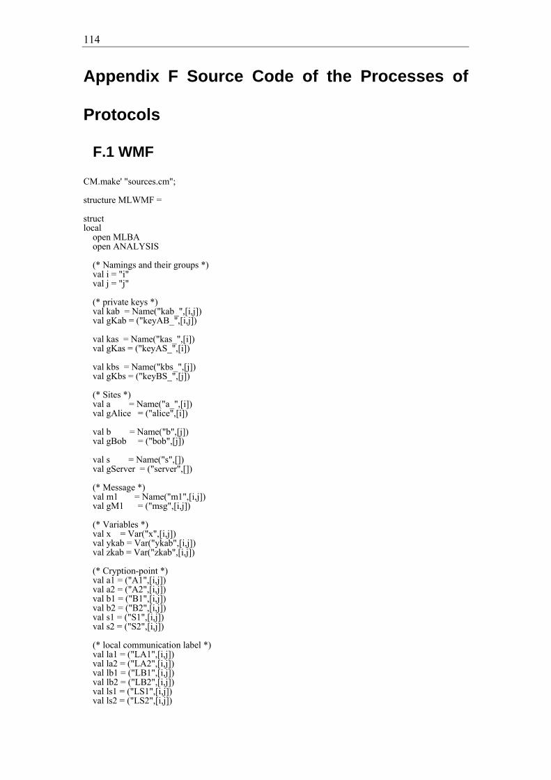
114
Appendix F Source Code of the Processes of
Protocols
F.1 WMF
CM.make' "sources.cm"; structure MLWMF = struct local open MLBA open ANALYSIS (* Namings and their groups *) val i = "i" val j = "j" (* private keys *) val kab = Name("kab_",[i,j]) val gKab = ("keyAB_",[i,j]) val kas = Name("kas_",[i]) val gKas = ("keyAS_",[i]) val kbs = Name("kbs_",[j]) val gKbs = ("keyBS_",[j]) (* Sites *) val a = Name("a_",[i]) val gAlice = ("alice",[i]) val b = Name("b",[j]) val gBob = ("bob",[j]) val s = Name("s",[]) val gServer = ("server",[]) (* Message *) val m1 = Name("m1",[i,j]) val gM1 = ("msg",[i,j]) (* Variables *) val x = Var("x",[i,j]) val ykab = Var("ykab",[i,j]) val zkab = Var("zkab",[i,j]) (* Cryption-point *) val a1 = ("A1",[i,j]) val a2 = ("A2",[i,j]) val b1 = ("B1",[i,j]) val b2 = ("B2",[i,j]) val s1 = ("S1",[i,j]) val s2 = ("S2",[i,j]) (* local communication label *) val la1 = ("LA1",[i,j]) val la2 = ("LA2",[i,j]) val lb1 = ("LB1",[i,j]) val lb2 = ("LB2",[i,j]) val ls1 = ("LS1",[i,j]) val ls2 = ("LS2",[i,j])

115
(* Sites *) val A = IPar("i",NATURAL3, Amb(a, IPar("j",NATURAL3, New(kab,gKab, Par(Amb(kas,Pre(Out(a), Pre(In(s), Par(Sendp([NX(a)]), Sendl([NX(b),NX(kab)],a1,[s1],la1) ) ) ) ), New(m1,gM1, Amb(kab,Pre(Out(a), Pre(In(b), Sendl([NX(m1)],a2,[b2],la2) ) ) ) ) ) (* Par *) ) (* New kab *) ) ) (* Ambient a *) ) (* IPar *) val B = IPar("j",NATURAL3, Amb(b, IPar("i",NATURAL3, Receivec([NX(a)],[zkab],kbs,b1,[s2],lb1, Receivec([],[x],zkab,b2,[a2],lb2,Nil) ) ) ) ) val S = Amb(s, IPar("i",NATURAL3, IPar("j",NATURAL3, Receivel([NX(a)],[], Receivec([NX(b)],[ykab],kas,s1,[a1],ls1, Amb(kbs, Pre(Out(s), Pre(In(b), Sendl([NX(a),NX(ykab)],s2,[b1],ls2) ) ) ) ) ) ) ) ) val P = INews([("i",NATURAL3)],a,gAlice, INews([("j",NATURAL3)],b,gBob, News(s,gServer, Par( INew([("i",NATURAL3)],kas,gKas, INew([("j",NATURAL3)],kbs,gKbs, Par(A, Par(B,S) ) ) ), Attacker )

116
) ) ) in fun analyse () = ANALYSIS.generate P "mlwmf" fun analyse1 P filename = ANALYSIS.generate P filename end end WMF Variant 1:
CM.make' "sources.cm"; structure MLWMF1 = struct local open MLBA open ANALYSIS (* Namings and their groups *) val i = "i" val j = "j" (* private keys *) val kab = Name("kab_",[i,j]) val gKab = ("keyAB_",[i,j]) val kas = Name("kas_",[i]) val gKas = ("keyAS_",[i]) val kbs = Name("kbs_",[j]) val gKbs = ("keyBS_",[j]) (* Sites *) val a = Name("a_",[i]) val gAlice = ("alice",[i]) val b = Name("b",[j]) val gBob = ("bob",[j]) val s = Name("s",[]) val gServer = ("server",[]) (* Message *) val m1 = Name("m1",[i,j]) val gM1 = ("msg",[i,j]) (* Variables *) val x = Var("x",[i,j]) val ykab = Var("ykab",[i,j]) val zkab = Var("zkab",[i,j]) (* Cryption-point *) val a1 = ("A1",[i,j]) val a2 = ("A2",[i,j]) val b1 = ("B1",[i,j]) val b2 = ("B2",[i,j]) val s1 = ("S1",[i,j]) val s2 = ("S2",[i,j]) (* local communication label *) val la1 = ("LA1",[i,j]) val la2 = ("LA2",[i,j]) val lb1 = ("LB1",[i,j]) val lb2 = ("LB2",[i,j]) val ls1 = ("LS1",[i,j]) val ls2 = ("LS2",[i,j])

117
(* Sites *) val A = IPar("i",NATURAL3, Amb(a, IPar("j",NATURAL3, New(kab,gKab, Par(Amb(kas,Pre(Out(a), Pre(In(s), Par(Sendp([NX(a)]), Sendl([NX(b),NX(kab)],a1,[s1],la1) ) ) ) ), New(m1,gM1, Amb(kab,Pre(Out(a), Pre(In(b), Sendl([NX(m1)],a2,[b2],la2) ) ) ) ) ) (* Par *) ) (* New kab *) ) ) (* Ambient a *) ) (* IPar *) val B = IPar("j",NATURAL3, Amb(b, IPar("i",NATURAL3, Receivel([NX(a)],[], Receivec([],[zkab],kbs,b1,[s2],lb1, Receivec([],[x],zkab,b2,[a2],lb2,Nil) ) ) ) ) ) val S = Amb(s, IPar("i",NATURAL3, IPar("j",NATURAL3, Receivel([NX(a)],[], Receivec([NX(b)],[ykab],kas,s1,[a1],ls1, Amb(kbs, Pre(Out(s), Pre(In(b), Par(Sendp([NX(a)]),Sendl([NX(ykab)],s2,[b1],ls2)) ) ) ) ) ) ) ) ) val P = INews([("i",NATURAL3)],a,gAlice, INews([("j",NATURAL3)],b,gBob, News(s,gServer, Par( INew([("i",NATURAL3)],kas,gKas, INew([("j",NATURAL3)],kbs,gKbs, Par(A, Par(B,S) ) ) ),

118
Attacker ) ) ) ) in fun analyse () = ANALYSIS.generate P "mlwmf_v1" fun analyse1 P filename = ANALYSIS.generate P filename end end WMF Variant 2:
CM.make' "sources.cm"; structure MLWMF2 = struct local open MLBA open ANALYSIS (* Namings and their groups *) val i = "i" val j = "j" (* private keys *) val kab = Name("kab_",[i,j]) val gKab = ("keyAB_",[i,j]) val kas = Name("kas_",[i]) val gKas = ("keyAS_",[i]) val kbs = Name("kbs_",[j]) val gKbs = ("keyBS_",[j]) (* Sites *) val a = Name("a_",[i]) val gAlice = ("alice",[i]) val b = Name("b",[j]) val gBob = ("bob",[j]) val s = Name("s",[]) val gServer = ("server",[]) (* Message *) val m1 = Name("m1",[i,j]) val gM1 = ("msg",[i,j]) (* Variables *) val x = Var("x",[i,j]) val ykab = Var("ykab",[i,j]) val zkab = Var("zkab",[i,j]) (* Cryption-point *) val a1 = ("A1",[i,j]) val a2 = ("A2",[i,j]) val b1 = ("B1",[i,j]) val b2 = ("B2",[i,j]) val s1 = ("S1",[i,j]) val s2 = ("S2",[i,j]) (* local communication label *) val la1 = ("LA1",[i,j]) val la2 = ("LA2",[i,j]) val lb1 = ("LB1",[i,j])

119
val lb2 = ("LB2",[i,j]) val ls1 = ("LS1",[i,j]) val ls2 = ("LS2",[i,j]) (* Sites *) val A = IPar("i",NATURAL3, Amb(a, IPar("j",NATURAL3, New(kab,gKab, Par(Amb(kas,Pre(Out(a), Pre(In(s), Par(Sendp([NX(a),NX(b)]), Sendl([NX(kab)],a1,[s1],la1) ) ) ) ), New(m1,gM1, Amb(kab,Pre(Out(a), Pre(In(b), Sendl([NX(m1)],a2,[b2],la2) ) ) ) ) ) (* Par *) ) (* New kab *) ) ) (* Ambient a *) ) (* IPar *) val B = IPar("j",NATURAL3, Amb(b, IPar("i",NATURAL3, Receivec([NX(a)],[zkab],kbs,b1,[s2],lb1, Receivec([],[x],zkab,b2,[a2],lb2,Nil) ) ) ) ) val S = Amb(s, IPar("i",NATURAL3, IPar("j",NATURAL3, Receivel([NX(a),NX(b)],[], Receivec([],[ykab],kas,s1,[a1],ls1, Amb(kbs, Pre(Out(s), Pre(In(b), Sendl([NX(a),NX(ykab)],s2,[b1],ls2) ) ) ) ) ) ) ) ) val P = INews([("i",NATURAL3)],a,gAlice, INews([("j",NATURAL3)],b,gBob, News(s,gServer, Par( INew([("i",NATURAL3)],kas,gKas, INew([("j",NATURAL3)],kbs,gKbs, Par(A, Par(B,S) ) )

120
), Attacker ) ) ) ) in fun analyse () = ANALYSIS.generate P "mlwmf_v2" fun analyse1 P filename = ANALYSIS.generate P filename end end
F.2 Needham Schroeder
CM.make' "sources.cm"; structure MLNHS = struct local open MLBA open ANALYSIS (* Namings and their groups *) val i = "i" val j = "j" (* private keys *) val kab = Name("kab_",[i,j]) val gKab = ("keyAB_",[i,j]) val kas = Name("kas_",[i]) val gKas = ("keyAS_",[i]) val kbs = Name("kbs_",[j]) val gKbs = ("keyBS_",[j]) (* Nounce or random number *) val ra = Name("ra_",[i,j]) val gRa = ("randomA_",[i,j]) val rb = Name("rb_",[i,j]) val gRb = ("randomB_",[i,j]) (* anonymous packet *) val p = Name("p_",[]) val gP = ("packet_",[]) (* Sites *) val a = Name("a_",[i]) val gAlice = ("alice",[i]) val b = Name("b",[j]) val gBob = ("bob",[j]) val s = Name("s",[]) val gServer = ("server",[]) (* Message *) val m1 = Name("m1",[i,j]) val gM1 = ("msg",[i,j]) (* Variables *) val xkab = Var("xkab",[i,j]) val xrb = Var("xrb",[i,j]) val yra = Var("yra",[i,j])

121
val zkab = Var("zkab",[i,j]) val zm = Var("zm",[i,j]) (* Cryption-point *) val a1 = ("A1",[i,j]) val a2 = ("A2",[i,j]) val a3 = ("A3",[i,j]) val a4 = ("A4",[i,j]) val b1 = ("B1",[i,j]) val b2 = ("B2",[i,j]) val b3 = ("B3",[i,j]) val b4 = ("B4",[i,j]) val s1 = ("S1",[i,j]) val s2 = ("S2",[i,j]) (* local communication label *) val la1 = ("LA1",[i,j]) val la2 = ("LA2",[i,j]) val la3 = ("LA3",[i,j]) val la4 = ("LA4",[i,j]) val lb1 = ("LB1",[i,j]) val lb2 = ("LB2",[i,j]) val lb3 = ("LB3",[i,j]) val lb4 = ("LB4",[i,j]) val ls1 = ("LS1",[i,j]) val ls2 = ("LS2",[i,j]) (* Sites *) val A = IPar("i",NATURAL3, Amb(a, IPar("j",NATURAL3, New(ra,gRa, Par(Amb(p,Pre(Out(a), Pre(In(s), Sendp([NX(a),NX(b),NX(ra)]) ) ) ), Par(Receivec([NX(a)],[xkab],kas,a1,[s1],la1, Receivec([],[xrb],xkab,a2,[b2],la2, Amb(xkab,Pre(Out(a), Pre(In(b), Sendl([NX(xrb),NX(xrb)],a3,[b3],la3) ) ) ) ) ), New(m1,gM1, Amb(xkab,Pre(Out(a), Pre(In(b), Sendl([NX(m1)],a4,[b4],la4) ) ) ) ) ) (* Par *) ) (* Par *) ) (* New ra *) ) ) (* Ambient a *) ) (* IPar *) val B = IPar("j",NATURAL3, Amb(b, IPar("i",NATURAL3, Receivec([NX(a)],[zkab],kbs,b1,[s2],lb1, New(rb,gRb, Par(

122
Amb(zkab,Pre(Out(b), Pre(In(a), Sendl([NX(rb)],b2,[a2],lb2) ) ) ), Receivec([NX(rb),NX(rb)],[],zkab,b3,[a3],lb3, Receivec([],[zm],zkab,b4,[a4],lb4,Nil) ) ) (* Par *) ) (* New *) ) (* Receivec *) ) ) ) val S = Amb(s, IPar("i",NATURAL3, IPar("j",NATURAL3, Receivel([NX(a),NX(b)],[yra], New(kab,gKab, Amb(kas, Pre(Out(s), Pre(In(a), Par( Sendl([NX(yra),NX(kab)],s1,[a1],ls1), Amb(kbs, Pre(Out(kas), Pre(Out(a), Pre(In(b), Sendl([NX(yra),NX(kab)],s1,[a1],ls1) ) ) ) ) (* Amb *) ) (* Par *) ) ) ) (* Amb *) ) (* New *) ) (* Receivec *) ) ) ) val P = INews([("i",NATURAL3)],a,gAlice, INews([("j",NATURAL3)],b,gBob, News(s,gServer, Par( New(p,gP, INew([("i",NATURAL3)],kas,gKas, INew([("j",NATURAL3)],kbs,gKbs, Par(A, Par(B,S) ) ) ) ), Attacker ) ) ) ) in fun analyse () = ANALYSIS.generate P "mlnhs" fun analyse1 P filename = ANALYSIS.generate P filename end end

123
Correcting the flaw
CM.make' "sources.cm"; structure MLNHS_COR = struct local open MLBA open ANALYSIS (* Namings and their groups *) (* Index *) val i = "i" val j = "j" (* private keys *) val kab = Name("kab_",[i,j]) val gKab = ("keyAB_",[i,j]) val kas = Name("kas_",[i]) val gKas = ("keyAS_",[i]) val kbs = Name("kbs_",[j]) val gKbs = ("keyBS_",[j]) (* Nounce or random number *) val ra = Name("ra_",[i,j]) val gRa = ("randomA_",[i,j]) val rb = Name("rb_",[i,j]) val gRb = ("randomB_",[i,j]) (* padding message to correct the flaw *) val u1 = Name("u1_",[i,j]) val gU1 = ("u1_",[i,j]) val u2 = Name("u2_",[i,j]) val gU2 = ("u2_",[i,j]) (* anonymous packet *) val p = Name("p_",[]) val gP = ("packet_",[]) (* Sites *) val a = Name("a_",[i]) val gAlice = ("alice",[i]) val b = Name("b",[j]) val gBob = ("bob",[j]) val s = Name("s",[]) val gServer = ("server",[]) (* Message *) val m1 = Name("m1",[i,j]) val gM1 = ("msg",[i,j]) (* Variables *) val xkab = Var("xkab",[i,j]) val xrb = Var("xrb",[i,j]) val yra = Var("yra",[i,j]) val zkab = Var("zkab",[i,j]) val zm = Var("zm",[i,j]) (* Cryption-point *) val a1 = ("A1",[i,j]) val a2 = ("A2",[i,j]) val a3 = ("A3",[i,j])

124
val a4 = ("A4",[i,j]) val b1 = ("B1",[i,j]) val b2 = ("B2",[i,j]) val b3 = ("B3",[i,j]) val b4 = ("B4",[i,j]) val s1 = ("S1",[i,j]) val s2 = ("S2",[i,j]) (* local communication label *) val la1 = ("LA1",[i,j]) val la2 = ("LA2",[i,j]) val la3 = ("LA3",[i,j]) val la4 = ("LA4",[i,j]) val lb1 = ("LB1",[i,j]) val lb2 = ("LB2",[i,j]) val lb3 = ("LB3",[i,j]) val lb4 = ("LB4",[i,j]) val ls1 = ("LS1",[i,j]) val ls2 = ("LS2",[i,j]) (* Sites *) val A = IPar("i",NATURAL3, Amb(a, IPar("j",NATURAL3, New(ra,gRa, Par(Amb(p,Pre(Out(a), Pre(In(s), Sendp([NX(a),NX(b),NX(ra)]) ) ) ), Par(Receivec([NX(a)],[xkab],kas,a1,[s1],la1, Receivec([NX(u1)],[xrb],xkab,a2,[b2],la2, Amb(xkab,Pre(Out(a), Pre(In(b), Sendl([NX(u2),NX(xrb),NX(xrb)],a3,[b3],la3) ) ) ) ) ), New(m1,gM1, Amb(xkab,Pre(Out(a), Pre(In(b), Sendl([NX(m1)],a4,[b4],la4) ) ) ) ) ) (* Par *) ) (* Par *) ) (* New ra *) ) ) (* Ambient a *) ) (* IPar *) val B = IPar("j",NATURAL3, Amb(b, IPar("i",NATURAL3, Receivec([NX(a)],[zkab],kbs,b1,[s2],lb1, New(rb,gRb, Par( Amb(zkab,Pre(Out(b), Pre(In(a), Sendl([NX(u1),NX(rb)],b2,[a2],lb2) ) ) ), Receivec([NX(u2),NX(rb),NX(rb)],[],zkab,b3,[a3],lb3,

125
Receivec([],[zm],zkab,b4,[a4],lb4,Nil) ) ) (* Par *) ) (* New *) ) (* Receivec *) ) ) ) val S = Amb(s, IPar("i",NATURAL3, IPar("j",NATURAL3, Receivel([NX(a),NX(b)],[yra], New(kab,gKab, Amb(kas, Pre(Out(s), Pre(In(a), Par( Sendl([NX(yra),NX(kab)],s1,[a1],ls1), Amb(kbs, Pre(Out(kas), Pre(Out(a), Pre(In(b), Sendl([NX(yra),NX(kab)],s2,[b1],ls2) ) ) ) ) (* Amb *) ) (* Par *) ) ) ) (* Amb *) ) (* New *) ) (* Receivec *) ) ) ) val P = INews([("i",NATURAL3)],a,gAlice, INews([("j",NATURAL3)],b,gBob, INew([("i",NATURAL3),("j",NATURAL3)],u1,gU1, INew([("i",NATURAL3),("j",NATURAL3)],u2,gU2, News(s,gServer, Par( New(p,gP, INew([("i",NATURAL3)],kas,gKas, INew([("j",NATURAL3)],kbs,gKbs, Par(A, Par(B,S) ) ) ) ), Attacker ) ) )) ) ) in fun analyse () = ANALYSIS.generate P "mlnhs_cor" fun analyse1 P filename = ANALYSIS.generate P filename end end

126
F.3 Otway-Rees.
CM.make' "sources.cm"; structure MLOTW = struct local open MLBA open ANALYSIS (* Namings and their groups *) (* Index *) val i = "i" val j = "j" (* private keys *) val kab = Name("kab_",[i,j]) val gKab = ("keyAB_",[i,j]) val kas = Name("kas_",[i]) val gKas = ("keyAS_",[i]) val kbs = Name("kbs_",[j]) val gKbs = ("keyBS_",[j]) (* Nounce or random number *) val n = Name("n_",[i,j]) val gN = ("nounceN_",[i,j]) val na = Name("na_",[i,j]) val gNa = ("nounceNa_",[i,j]) val nb = Name("nb_",[i,j]) val gNb = ("nounceNb_",[i,j]) (* Sites *) val a = Name("a_",[i]) val gAlice = ("alice",[i]) val b = Name("b",[j]) val gBob = ("bob",[j]) val s = Name("s",[]) val gServer = ("server",[]) (* Message *) val m1 = Name("m1",[i,j]) val gM1 = ("msg",[i,j]) (* Variables *) val xkab = Var("xkab",[i,j]) val yn = Var("yn",[i,j]) val yna = Var("yna",[i,j]) val ynb = Var("ynb",[i,j]) val zn = Var("zn",[i,j]) val zkab = Var("zkab",[i,j]) val zm = Var("zm",[i,j]) (* Cryption-point *) val a1 = ("A1",[i,j]) val a2 = ("A2",[i,j]) val a3 = ("A3",[i,j]) val a4 = ("A4",[i,j]) val b1 = ("B1",[i,j]) val b2 = ("B2",[i,j]) val b3 = ("B3",[i,j]) val b4 = ("B4",[i,j])

127
val s1 = ("S1",[i,j]) val s2 = ("S2",[i,j]) val s3 = ("S3",[i,j]) val s4 = ("S4",[i,j]) (* local communication label *) val la1 = ("LA1",[i,j]) val la2 = ("LA2",[i,j]) val la3 = ("LA3",[i,j]) val lb1 = ("LB1",[i,j]) val lb2 = ("LB2",[i,j]) val lb3 = ("LB3",[i,j]) val ls1 = ("LS1",[i,j]) val ls2 = ("LS2",[i,j]) val ls3 = ("LS3",[i,j]) val ls4 = ("LS4",[i,j]) (* Sites *) val A = IPar("i",NATURAL3, Amb(a, IPar("j",NATURAL3, New(n,gN,New(na,gNa, Par(Amb(kas,Pre(Out(a), Pre(In(b), Par(Sendp([NX(n)]), Pre(Out(b), Pre(In(s), Par(Sendp([NX(n)]), Sendl([NX(a),NX(b),NX(n),NX(na)],a1,[s1],la1) ) ) ) ) ) ) ), Receivel([NX(n)],[], Receivec([NX(na)],[xkab],kas,a2,[s4],la2, New(m1,gM1, Amb(xkab,Pre(Out(a), Pre(In(b), Sendl([NX(m1)],a3,[b3],la3) ) ) ) ) ) ) ) (* Par *) )) (* New n and na *) ) ) (* Ambient a *) ) (* IPar *) val B = IPar("j",NATURAL3, Amb(b, IPar("i",NATURAL3, Receivel([],[zn], New(nb,gNb, Par( Amb(kbs,Pre(Out(b), Pre(In(s), Sendl([NX(a),NX(b),NX(zn),NX(nb)],b1,[s2],lb1) ) ) ), Receivel([],[zn], Receivec([NX(nb)],[zkab],kbs,b2,[s3],lb2, Receivec([],[zm],zkab,b3,[a3],lb3,Nil)

128
) ) ) (* Par *) ) (* New *) ) (* Receivel *) ) ) ) val S = Amb(s, IPar("i",NATURAL3, IPar("j",NATURAL3, Receivel([],[yn], Receivec([NX(a),NX(b),NX(yn)],[yna],kas,s1,[a1],ls1, Receivec([NX(a),NX(b),NX(yn)],[ynb],kbs,s2,[b1],ls2, New(kab,gKab, Amb(kbs, Pre(Out(s), Pre(In(b), Par( Sendp([NX(yn)]), Par( Sendl([NX(ynb),NX(kab)],s3,[b2],ls3), Amb(kas, Pre(Out(kbs), Pre(Out(b), Pre(In(a), Par( Sendp([NX(yn)]), Sendl([NX(yna),NX(kab)],s4,[a2],ls4) ) ) ) ) (* Amb *) ) (* Sendl *) ) (* Par *) ) (* Par *) ) ) ) (* Amb *) ) (* New *) ) ) ) (* Receivel *) ) ) ) val P = INews([("i",NATURAL3)],a,gAlice, INews([("j",NATURAL3)],b,gBob, News(s,gServer, Par( INew([("i",NATURAL3)],kas,gKas, INew([("j",NATURAL3)],kbs,gKbs, Par(A, Par(B,S) ) ) ), Attacker ) ) ) ) in fun analyse () = ANALYSIS.generate P "mlotw" fun analyse1 P filename = ANALYSIS.generate P filename end end

129
F.4 Yahalom
CM.make' "sources.cm"; structure MLYAH = struct local open MLBA open ANALYSIS (* Namings and their groups *) (* Index *) val i = "i" val j = "j" (* private keys *) val kab = Name("kab_",[i,j]) val gKab = ("keyAB_",[i,j]) val kas = Name("kas_",[i]) val gKas = ("keyAS_",[i]) val kbs = Name("kbs_",[j]) val gKbs = ("keyBS_",[j]) (* anonymous packet *) val p = Name("p_",[]) val gP = ("packet_",[]) (* Nounce or random number *) val na = Name("na_",[i,j]) val gNa = ("nounceNa_",[i,j]) val nb = Name("nb_",[i,j]) val gNb = ("nounceNb_",[i,j]) (* Sites *) val a = Name("a_",[i]) val gAlice = ("alice",[i]) val b = Name("b",[j]) val gBob = ("bob",[j]) val s = Name("s",[]) val gServer = ("server",[]) (* Message *) val m1 = Name("m1",[i,j]) val gM1 = ("msg",[i,j]) (* Variables *) val xkab = Var("xkab",[i,j]) val xnb = Var("xnb",[i,j]) val yn = Var("yn",[i,j]) val yna = Var("yna",[i,j]) val ynb = Var("ynb",[i,j]) val zna = Var("zna",[i,j]) val zkab = Var("zkab",[i,j]) val zm = Var("zm",[i,j]) (* Cryption-point *) val a1 = ("A1",[i,j]) val a2 = ("A2",[i,j]) val a3 = ("A3",[i,j]) val b1 = ("B1",[i,j])

130
val b2 = ("B2",[i,j]) val b3 = ("B3",[i,j]) val b4 = ("B4",[i,j]) val s1 = ("S1",[i,j]) val s2 = ("S2",[i,j]) val s3 = ("S3",[i,j]) (* local communication label *) val la1 = ("LA1",[i,j]) val la2 = ("LA2",[i,j]) val la3 = ("LA3",[i,j]) val lb1 = ("LB1",[i,j]) val lb2 = ("LB2",[i,j]) val lb3 = ("LB3",[i,j]) val lb4 = ("LB4",[i,j]) val ls1 = ("LS1",[i,j]) val ls2 = ("LS2",[i,j]) val ls3 = ("LS3",[i,j]) (* Sites *) val A = IPar("i",NATURAL1, Amb(a, IPar("j",NATURAL1, New(na,gNa, Par(Amb(p,Pre(Out(a), Pre(In(s), Sendp([NX(a),NX(na)]) ) ) ), Par( Receivec([NX(b),NX(na)],[xkab,xnb],kas,a1,[s2],la1, Amb(xkab,Pre(Out(a), Pre(In(b), Sendl([NX(xnb)],a2,[b3],la2) ) ) ) ), New(m1,gM1, Amb(xkab,Pre(Out(a), Pre(In(b), Sendl([NX(m1)],a3,[b4],la3) ) ) ) ) ) ) (* Par *) ) (* New na *) ) ) (* Ambient a *) ) (* IPar *) val B = IPar("j",NATURAL1, Amb(b, IPar("i",NATURAL1, Receivel([NX(a)],[zna], New(nb,gNb, Par( Amb(kbs,Pre(Out(b), Pre(In(s), Par(Sendp([NX(b)]), Sendl([NX(a),NX(zna),NX(nb)],b1,[s1],lb1) ) ) ) ), Receivec([NX(a)],[zkab],kbs,b2,[s3],lb2,

131
Receivec([NX(nb)],[],zkab,b3,[a2],lb3, Receivec([],[zm],zkab,b4,[a3],lb4,Nil) ) ) ) (* Par *) ) (* New *) ) (* Receivel *) ) ) ) val S = Amb(s, IPar("i",NATURAL1, IPar("j",NATURAL1, Receivel([NX(b)],[], Receivec([NX(a)],[yna,ynb],kbs,s1,[b1],ls1, New(kab,gKab, Amb(kas, Pre(Out(s), Pre(In(a), Par( Sendl([NX(b),NX(yna),NX(kab),NX(ynb)],s2,[a1],ls2), Amb(kbs, Pre(Out(kas), Pre(Out(a), Pre(In(b), Sendl([NX(a),NX(kab)],s3,[b2],ls3) ) ) ) ) (* Amb *) ) (* Par *) ) ) ) (* Amb *) ) (* New *) ) ) (* Receivel *) ) ) ) val P = INews([("i",NATURAL1)],a,gAlice, INews([("j",NATURAL1)],b,gBob, News(s,gServer, Par( INew([("i",NATURAL1)],kas,gKas, INew([("j",NATURAL1)],kbs,gKbs, New(p,gP, Par(A, Par(B,S) ) ) ) ), Attacker ) ) ) ) in fun analyse () = ANALYSIS.generate P "mlyah" fun analyse1 P filename = ANALYSIS.generate P filename end end

132
F.5 Andrew Secure RPC
CM.make' "sources.cm"; structure MLANDREW = struct local open MLBA open ANALYSIS (* Namings and their groups *) (* Index *) val i = "i" val j = "j" (* private keys *) val kab = Name("kab_",[i,j]) val gKab = ("keyAB_",[i,j]) val kab' = Name("kab'_",[i,j]) val gKab'= ("keyAB'_",[i,j]) (* Nounce or random number *) val na = Name("na_",[i,j]) val gNa = ("nounceA_",[i,j]) val nb = Name("nb_",[i,j]) val gNb = ("nounceB_",[i,j]) val nb' = Name("nb'_",[i,j]) val gNb' = ("nounceb'_",[i,j]) (* padding message to correct the flaw *) (* val u1 = Name("u1_",[i,j]) val gU1 = ("u1_",[i,j]) val u2 = Name("u2_",[i,j]) val gU2 = ("u2_",[i,j]) *) (* anonymous packet *) (*val p = Name("p_",[]) val gP = ("packet_",[]) *) (* Sites *) val a = Name("a_",[i]) val gAlice = ("alice",[i]) val b = Name("b",[j]) val gBob = ("bob",[j]) (* Message *) val m1 = Name("m1",[i,j]) val gM1 = ("msg",[i,j]) (* Variables *) val xnb = Var("xnb",[i,j]) val xkab'= Var("xkab'",[i,j]) val xnb' = Var("xnb'",[i,j]) val yna = Var("yna",[i,j]) val ym = Var("ym",[i,j]) (* Cryption-point *) val a1 = ("A1",[i,j]) val a2 = ("A2",[i,j]) val a3 = ("A3",[i,j]) val a4 = ("A4",[i,j]) val a5 = ("A5",[i,j]) val b1 = ("B1",[i,j])

133
val b2 = ("B2",[i,j]) val b3 = ("B3",[i,j]) val b4 = ("B4",[i,j]) val b5 = ("B5",[i,j]) (* local communication label *) val la1 = ("LA1",[i,j]) val la2 = ("LA2",[i,j]) val la3 = ("LA3",[i,j]) val la4 = ("LA4",[i,j]) val la5 = ("LA5",[i,j]) val lb1 = ("LB1",[i,j]) val lb2 = ("LB2",[i,j]) val lb3 = ("LB3",[i,j]) val lb4 = ("LB4",[i,j]) val lb5 = ("LB5",[i,j]) (* Sites *) val A = IPar("i",NATURAL3, Amb(a, IPar("j",NATURAL3, New(na,gNa, Par(Amb(kab,Pre(Out(a), Pre(In(b), Par(Sendp([NX(a)]), Sendl([NX(na)],a1,[b1],la1) ) ) ) ), Par(Receivec([NX(na),NX(na)],[xnb],kab,a2,[b2],la2, Amb(kab,Pre(Out(a), Pre(In(b), Sendl([NX(xnb),NX(xnb)],a3,[b3],la3) ) ) ) ), New(m1,gM1, Receivec([],[xkab',xnb'],kab,a4,[b4],la4, Amb(xkab',Pre(Out(a), Pre(In(b), Sendl([NX(m1)],a5,[b5],la5) ) ) ) ) ) ) (* Par *) ) (* Par *) ) (* New na *) ) ) (* Ambient a *) ) (* IPar *) val B = IPar("j",NATURAL3, Amb(b, IPar("i",NATURAL3, Receivel([NX(a)],[], Receivec([],[yna],kab,b1,[a1],lb1, New(nb,gNb, Par( Amb(kab,Pre(Out(b), Pre(In(a), Sendl([NX(yna),NX(yna),NX(nb)],b2,[a2],lb2) ) ) ), Receivec([NX(nb),NX(nb)],[],kab,b3,[a3],lb3,

134
New(kab',gKab', New(nb',gNb', Par( Amb(kab,Pre(Out(b), Pre(In(a), Sendl([NX(kab'),NX(nb')],b4,[a4],lb4) ) ) ), Receivec([],[ym],kab',b5,[a5],lb5,Nil) ) ) ) ) (* Receivec *) ) (* Par *) ) (* New *) ) (* Receivec *) ) (* Receivel *) ) ) ) val P = INews([("i",NATURAL3)],a,gAlice, INews([("j",NATURAL3)],b,gBob, (*INew([("i",NATURAL3),("j",NATURAL3)],u1,gU1, INew([("i",NATURAL3),("j",NATURAL3)],u2,gU2,*) Par( INew([("i",NATURAL3),("j",NATURAL3)],kab,gKab, Par(A,B) ), Attacker ) (*))*) ) ) in fun analyse () = ANALYSIS.generate P "mlAndrew" fun analyse1 P filename = ANALYSIS.generate P filename end end Correcting the flaw
CM.make' "sources.cm"; structure MLANDREW_COR = struct local open MLBA open ANALYSIS (* Namings and their groups *) (* Index *) val i = "i" val j = "j" (* private keys *) val kab = Name("kab_",[i,j]) val gKab = ("keyAB_",[i,j]) val kab' = Name("kab'_",[i,j]) val gKab'= ("keyAB'_",[i,j]) (* Nounce or random number *) val na = Name("na_",[i,j]) val gNa = ("nounceA_",[i,j])

135
val nb = Name("nb_",[i,j]) val gNb = ("nounceB_",[i,j]) val nb' = Name("nb'_",[i,j]) val gNb' = ("nounceb'_",[i,j]) (* padding message to correct the flaw *) val u1 = Name("u1_",[i,j]) val gU1 = ("u1_",[i,j]) val u2 = Name("u2_",[i,j]) val gU2 = ("u2_",[i,j]) val u3 = Name("u3_",[i,j]) val gU3 = ("u3_",[i,j]) val u4 = Name("u4_",[i,j]) val gU4 = ("u4_",[i,j]) (* anonymous packet *) (*val p = Name("p_",[]) val gP = ("packet_",[]) *) (* Sites *) val a = Name("a_",[i]) val gAlice = ("alice",[i]) val b = Name("b",[j]) val gBob = ("bob",[j]) (* Message *) val m1 = Name("m1",[i,j]) val gM1 = ("msg",[i,j]) (* Variables *) val xnb = Var("xnb",[i,j]) val xkab'= Var("xkab'",[i,j]) val xnb' = Var("xnb'",[i,j]) val yna = Var("yna",[i,j]) val ym = Var("ym",[i,j]) (* Cryption-point *) val a1 = ("A1",[i,j]) val a2 = ("A2",[i,j]) val a3 = ("A3",[i,j]) val a4 = ("A4",[i,j]) val a5 = ("A5",[i,j]) val b1 = ("B1",[i,j]) val b2 = ("B2",[i,j]) val b3 = ("B3",[i,j]) val b4 = ("B4",[i,j]) val b5 = ("B5",[i,j]) (* local communication label *) val la1 = ("LA1",[i,j]) val la2 = ("LA2",[i,j]) val la3 = ("LA3",[i,j]) val la4 = ("LA4",[i,j]) val la5 = ("LA5",[i,j]) val lb1 = ("LB1",[i,j]) val lb2 = ("LB2",[i,j]) val lb3 = ("LB3",[i,j]) val lb4 = ("LB4",[i,j]) val lb5 = ("LB5",[i,j]) (* Sites *) val A = IPar("i",NATURAL3, Amb(a, IPar("j",NATURAL3, New(na,gNa, Par(Amb(kab,Pre(Out(a), Pre(In(b),

136
Par(Sendp([NX(a)]), Sendl([NX(u1),NX(na)],a1,[b1],la1) ) ) ) ), Par(Receivec([NX(u2),NX(na),NX(na)],[xnb],kab,a2,[b2],la2, Amb(kab,Pre(Out(a), Pre(In(b), Sendl([NX(u3),NX(xnb),NX(xnb)],a3,[b3],la3) ) ) ) ), New(m1,gM1, Receivec([NX(u4)],[xkab',xnb'],kab,a4,[b4],la4, Amb(xkab',Pre(Out(a), Pre(In(b), Sendl([NX(m1)],a5,[b5],la5) ) ) ) ) ) ) (* Par *) ) (* Par *) ) (* New na *) ) ) (* Ambient a *) ) (* IPar *) val B = IPar("j",NATURAL3, Amb(b, IPar("i",NATURAL3, Receivel([NX(a)],[], Receivec([NX(u1)],[yna],kab,b1,[a1],lb1, New(nb,gNb, Par( Amb(kab,Pre(Out(b), Pre(In(a), Sendl([NX(u2),NX(yna),NX(yna),NX(nb)],b2,[a2],lb2) ) ) ), Receivec([NX(u3),NX(nb),NX(nb)],[],kab,b3,[a3],lb3, New(kab',gKab', New(nb',gNb', Par( Amb(kab,Pre(Out(b), Pre(In(a), Sendl([NX(u4),NX(kab'),NX(nb')],b4,[a4],lb4) ) ) ), Receivec([],[ym],kab',b5,[a5],lb5,Nil) ) ) ) ) (* Receivec *) ) (* Par *) ) (* New *) ) (* Receivec *) ) (* Receivel *) ) ) ) val P = INews([("i",NATURAL3)],a,gAlice, INews([("j",NATURAL3)],b,gBob,

137
Par( INew([("i",NATURAL3),("j",NATURAL3)],u1,gU1, INew([("i",NATURAL3),("j",NATURAL3)],u2,gU2, INew([("i",NATURAL3),("j",NATURAL3)],u3,gU3, INew([("i",NATURAL3),("j",NATURAL3)],u4,gU4, INew([("i",NATURAL3),("j",NATURAL3)],kab,gKab, Par(A,B) ) )))), Attacker ) ) ) in fun analyse () = ANALYSIS.generate P "mlAndrew_cor" fun analyse1 P filename = ANALYSIS.generate P filename end end

138
Appendix G Source Code of Testing
The sml code of the tests of all configurations have been uploaded to the following webpage:
http://www.student.dtu.dk/~s030998/content/research/master_thesis.htm
for your reference.

139
Appendix G List of Figures
Figure 1-1: An example of a network with hierarchical structure .................................1
Figure 2-1: Tree structure of the network shown in Figure 1-1.....................................5
Figure 2-2: Ambient structure of the network in Figure 1-1. ........................................6
Figure 6-1: Ambient structure of Configuration 1.......................................................71
Figure 6-2: Ambient structure of Configuration 2.......................................................71
Figure 6-3: Ambient structure of Configuration 3.......................................................73
Figure 6-4: Ambient structure of Configuration 4.......................................................79
Figure 6-5: Ambient structure of Configuration 5.......................................................81
Figure 6-6: Ambient structure of Configuration 6.......................................................82
Figure 6-7: Ambient structure of Configuration 7.......................................................83
Figure 6-8: Ambient structure of Configuration 8.......................................................83

140
Appendix H List of Tables
Table 2-1: The syntax of ABoxed Ambients .................................................................7
Table 2-2: Structural Congruence; P P′≡ ..................................................................11
Table 2-3: Free names; fn(P). ......................................................................................11
Table 2-4: Free variables; fv(P). ..................................................................................12
Table 2-5: Transition relation (1); P P′→R ; parameterized on R.............................12
Table 2-6: Transition relation (2); P P′→R ; parameterized on R.............................14
Table 2-7: Well-formedness of site processes with respect to Γ : Γ wfs(P★) ...........20
Table 2-8: Well-formedness of packet processes with respect to Γ : Γ wfp(P★) ......21
Table 2-9: WMF in ABoxed Ambients .......................................................................23
Table 3-1: Analysis specification (Part 1): ( , , ) :Pµγ κ ρ ϕ ......................................31
Table 3-2: Functions ρN and ρM ...............................................................................31
Table 3-3: Closure conditions in ( )ϕ µ and out ( )ϕ µ ......................................................32
Table 3-4: Analysis specification (Part 2): ( , , ) :Pµγ κ ρ ϕ ......................................34
Table 4-1: Adjusted Dolev-Yao condition...................................................................40
Table 5-1: Verbose formulation of the analysis...........................................................47
Table 5-2: Analysis with new environment functions , and Γ S P . ...........................50
Table 5-3: Encoding annotations in the analysis .........................................................52
Table 5-4: Abstract syntax of ALFP clauses ...............................................................53
Table 5-5: Semantics of ALFP clauses........................................................................54
Table 5-6: The generation function (1). .......................................................................56
Table 5-7: The generation function (2). .......................................................................57
Table 6-1: WMF protocol and Secure Login protocol.................................................68
Table 6-2: Process for Test 1 of Configuration 2 ........................................................72
Table 6-3: Process for Test 1 of Configuration 3 ........................................................74
Table 6-4: Process for Test 2 of Configuration 3 ........................................................77
Table 6-5: Process for Test 3 of Configuration 3 ........................................................78
Table 6-6: The experiment results for Test 1 of Configuration 4. ...............................79
Table 6-7: The experiment results for Test 1 of Configuration 5. ...............................81
Table 6-8: The experiment results for Test 1 of Configuration 6. ...............................82

141
Bibliography
[1] Flemming Nielson, Hanne Riis Nielson, Chris Hankin. Principles of Program Analysis. Springer-Verlag, 1999. [2] C. Bodei, M. Buchholtz, P. Degano, F. Nielson, H. Riis Nielson. Static Validation of Security Protocols (to appear), Journal of Computer Security, 2005. [3] H. Riis Nielson, F. Nielson, M. Buchholtz. Security for Mobility, Foundations of Security Analysis and Design II - FOSAD 2001/2002 Tutorial Lectures, vol. 2946, pp. 207-265, 2004. [4] M. Abadi and A. D. Gordon. A calculus for cryptographic protocols – The Spi calculus. Information and Computation, 148(1):1-70, 1999. [5] L. Cardelli and A.D. Gordon. Mobile ambients. In Proc. of FoSSaCS'98, LNCS 1378, pages 140-155. Springer, 1998. [6] L. Cardelli and A. D. Gordon. Mobile Ambients. Theoretical Computer Science, 240(1):177-213, 2000. [7] D. Dolev and A. Yao. On the security of public key protocols. IEEE Transactions on Information Theory, 29(2):198–208, 1983. [8] M. Bugliesi, G. Castagna, and S. Crafa. Boxed Ambients. In Theoretical Aspects in Computer Science (TACS 2001), volume 2215 of Lecture Notes in Computer Science, pages 37-63. Springer, 2001. [9] M. Bugliesi, G. Castagna, and S. Crafa. Boxed Ambients. Reasoning about security in Mobile Ambients. In CONCUR 2001 – Concurrency Theory, volume 2154 of Lecture Notes in Computer Science, pages 102-120. Springer, 2001. [10] F. Nielson, H. Riis Nielson, R.R. Hansen. Validating firewalls using flow logics. Theoretical Computer Science, 283(2):381-418, 2002. [11] F. Nielson, H. Riis Nielson, R.R. Hansen, and J.G. Jensen. Validating firewalls in Mobile Ambients. In CONCUR 1999 – Concurrency Theory, volume 1664 of Lecture Notes in Computer Science, pages 463-477. Springer, 1999. [12] H. Sun. User’s Guide for the Succinct Solver (V2.0). Draft, 2003. http://www2.imm.dtu.dk/cs_SuccinctSolver/userGuide.pdf . [13] F. Nielson, H. Seidl, and H. Riis Nielson. A Succinct Solver for ALFP, Nordic journal of computing, 2002(9), 2002. [14] H. Riis Nielson and F.Nielson. Flow Logic: a multi-paradigmatic approach to static analysis. In The Essence of Computation: Complexity, Analysis, Transformation, Lecture Notes in Computer Science 2566.pp 223-244. Springer, 2002.

142
[15] M.S Hecht. Flow Analysis of Computer Programs. North Holland, 1977. [16] N. Heintze. Set-based analysis of ML programs. In Proc. LFP ’94, pages 306-317, 1994. [17] P. Cousot and R. Cousot. Abstract Interpretation: a Unified Lattice Model for Static Analysis of Programs by Construction or Approximation of Fixpoints. In Proc. POPL ’77, pages 238-252. ACM Press, 1977. [18] R. Milner. A theory of type polymorphism in programming. Journal of Computer Systems, 17:348-375, 1978. [19] F. Nielson and H. Riis Nielson. Infinitary control flow analysis: a collecting semantics for closure analysis. In Proc. POPL ’97, pages 332-345. ACM Press, 1997. [20] Konstantino Saganos, Terrance Swift, David S. Warren, Juliana Freire, Prasad Rao, Boaqiu Cui, and Ernie Johnson. The XSB System - Version 2.5 – Programmers Manual, March 2002. [21] Konstantinos F. Sagonas, Terrance Swift, and David Scott Warren. Xsb as an e_cient deductive database engine. In Richard T. Snodgrass and Marianne Winslett, editors, Proceedings of the 1994 ACM SIGMOD International Conference on Management of Data, Minneapolis, Minnesota, May 24-27, 1994, pages 442{453. ACM Press, 1994. [22] H. Pilegaard, A feasibility Study: The Succinct Solver v2.0, XSB Prolog v2.6, and Flow-Logic Based Program Analysis for Carmel, 2003. [23] R.R.Hansen, A Prototype Tool for JavaCard Firewall Analysis, Nordic Workshop on Secure IT-Systems, 2002. [24] M. Buchholtz. Implementing Control Flow Analysis for security protocols, 2003. [25] J. Kelsey, B. Schneier, and D. Wagner. Protocol Interactions and the Chosen Protocol Attack, Security Protocols, 5th International Workshop April 1997 Proceedings, Springer-Verlag, 1998, pp. 91-104. [26] F.Levi and S. Maffeis. An abstract interpretation framework for analyzing Mobile Ambients. In Static Analysis, 8th International Symposium, SAS 2001, pages 395-411. Springer, 2001. [27] D. Otway and O. Rees. Efficient and timely mutual authentication. ACM Operating Systems Review, 21(1):8-10, 1987. [28] M. Satyanarayanan. Integrating security in a large distributed system. ACM ToCS, 7(3):247-280, 1989. [29] M. Burrows, M. Abadi, and R. Needham. A logic of Authentication. ACM Transactions on Computer Systems, pages 18-36, 1990.

143
[30] R.M. Needham and M.D. Schroeder. Using encryption for authentication in large networks of computers. Communications of the ACM, 21(12):993-999, 1978. [31] M. Abadi and A. D. Gordon. A calculus for cryptographic protocols – The Spi calculus. Information and Computation 148, 1:1-70, 1999. [32] F. Levi and D. Sangiorgi. Controlling interference in ambients. In Proceedings of the 27th ACM SIGPLAN-SIGACT Symposium on Principles of Programming Languages (POPL 2000), pages 352-364. ACM Press, 2000. [33] Hanne Riis Nielson, Flemming Nielson and Henrik Pilegaard. Spatial
Analysis of BioAmbients, to appear at Static Analysis Symposium (SAS04), Springer
Verlag, 2004.
[34] Han Gao. Using the Succinct Solver to Implement Flow Logic Specifications of Classical Data Flow Analyses, Master’s Thesis, 2004. [35] David Basin, Sebastian Mödersheim, Luca Viganò. OFMC:A symbolicmodel checker for security protocols, International Journal of Information Security, pages 181-208, Springer Verlag, 2005.
[36] F. J. Thayer Fabrega, J. Herzog, and J. D. Guttman, ``Strand spaces: Why is a security protocol correct?,'' in 1998 IEEE Symposium on Security and Privacy, IEEE Computer Society Press, May 1998. [37] C. Bodei, P. Degano, F. Nielson, and H. Riis Nielson. Static analysis for secrecy and non-interference in networks of processes. In Proc. PaCT’01, number 2127 in Lecture Notes in Computer Science, pages 27-41. Springer-Verlag, 2001.