PREFACE AND ACKNOWLEDGEMENT - Statistical Service Profile in Ghana... · ii PREFACE AND...
90
Transcript of PREFACE AND ACKNOWLEDGEMENT - Statistical Service Profile in Ghana... · ii PREFACE AND...

ii
PREFACE AND ACKNOWLEDGEMENT
This publication presents the latest analysis of the living conditions of Ghanaian households
and the poverty profile based on the sixth round of the Ghana Living Standards Survey
(GLSS6) conducted in 2012/2013. Five rounds of the Ghana Living Standards Survey have
been conducted in the past (1987/88, 1988/89, 1991/92, 1998/99 and 2005/06) each covering
a nationally representative sample of households interviewed over a period of twelve months.
The report covers three different dimensions of poverty namely: consumption poverty, lack
of access to assets and services and human development. The report analyzes macroeconomic
developments in the country since 2005, focusing on Growth in Gross Domestic Product
(GDP), trends in inflation, balance of payments and public expenditures. It also discusses
social protection interventions aimed at reducing poverty and programmes being
implemented towards the attainment of the Millennium Development Goals (MDGs).
As a result of the rebasing of the Consumer Price Index (CPI) basket in 2012, the
introduction of new consumer items onto the Ghanaian market and changes in household
consumption, the report presents the poverty profile of households in 2012/2013 and only
attempts to compare the current levels of poverty with those measured in round five of the
GLSS.
The Ghana Statistical Service wishes to acknowledge the contribution of the Government of
Ghana, the UK Department for International Development (UK-DFID), the World Bank,
UNICEF, UNFPA and International Labour Organization (ILO), who provided both technical
and financial support towards the successful implementation of the GLSS6 project.
The Service would also like to acknowledge the invaluable contributions of Xiao Xye and
Vasco Molini (both consultants from the World Bank), Lynn Henderson of DFID, Kofi
Agyeman-Duah, Anthony Amuzu, Abena Osei-Akoto, Jacqueline Anum, Samilia Mintah,
Yaw Misefa, Appiah Kusi-Boateng, Anthony Krakah, Asuo Afram, Francis Bright Mensah
and Patrick Adjovor all of the Statistical Service who worked tirelessly with the consultants
to produce this report under the overall guidance and supervision of Dr. Philomena Nyarko,
the Government Statistician.
DR. PHILOMENA NYARKO
GOVERNMENT STATISTICIAN
August 2014

iii
TABLE OF CONTENT
PREFACE AND ACKNOWLEDGEMENT ......................................................................... ii
LIST OF TABLES ................................................................................................................... v
LIST OF FIGURES ............................................................................................................... vii
EXECUTIVE SUMMARY .................................................................................................... ix
CHAPTER ONE: THE ECONOMIC CONTEXT .............................................................. 1 1.1 Gross Domestic Product (GDP), 2005-2013 ............................................................... 1 1.2 Trends in inflation (2005-2013) .................................................................................. 3
1.3 Balance of payments (2005-2013) .............................................................................. 3 1.4 Public expenditures (2005-2013) ................................................................................ 4 1.5 Social interventions ..................................................................................................... 4 1.6 Summary ..................................................................................................................... 4
CHAPTER TWO: CONSUMPTION POVERTY, METHODOLOGY AND
MEASUREMENT................................................................................ 5 2.1 Introduction ................................................................................................................. 5
2.2 Data sources ................................................................................................................ 5
2.3 Construction of the standard of living measure .......................................................... 5 2.4 Rebasing of the standard of living measurement ........................................................ 6 2.5 Rebasing the consumption basket and construction of the Poverty Line .................... 7
2.6 Summary ..................................................................................................................... 7
CHAPTER THREE: PROFILE OF CONSUMPTION POVERTY ................................. 9 3.1 Introduction ................................................................................................................. 9 3.2 Poverty incidence and poverty gap ............................................................................. 9 3.3 Extreme Poverty in Ghana ........................................................................................ 12
3.4 Poverty in Administrative Regions ........................................................................... 13 3.5 Summary ................................................................................................................... 17
CHAPTER FOUR: COVARIATE ANALYSIS ................................................................. 18 4.1 Decomposition of Poverty ......................................................................................... 18
4.2 Poverty by economic activity and gender of household head ................................... 18 4.3 Poverty and educational level of household head ..................................................... 20
4.4 Welfare distribution (Inequality analysis) in Ghana ................................................. 21 4.5 Growth incidence in Ghana: Is Ghana’s economic growth pro-poor? ...................... 22
4.6 Summary ................................................................................................................... 25
CHAPTER FIVE: HOUSEHOLD ASSETS ...................................................................... 26 5.1 Introduction ............................................................................................................... 26 5.2 Asset Ownership ....................................................................................................... 26 5.3 Summary ................................................................................................................... 30
CHAPTER SIX: ACCESS TO SERVICES ....................................................................... 31 6.1 Introduction ............................................................................................................... 31 6.2 Household access to utilities and sanitation facilities ............................................... 31 6.3 Summary ................................................................................................................... 33
CHAPTER SEVEN: HUMAN DEVELOPMENT ............................................................ 34 7.1 Introduction ............................................................................................................... 34 7.2 Access to health services ........................................................................................... 34 7.3 Access to education ................................................................................................... 37 7.4 Summary ................................................................................................................... 43

iv
CHAPTER EIGHT: CONCLUSION ................................................................................. 44 Appendix 1: Consumption Poverty Indices ..................................................................... 46 Appendix 2: Household Assets ........................................................................................ 51 Appendix 3: Household Access To Services ................................................................... 55 Appendix 4: Human Development Tables ...................................................................... 60
Appendix 5: Consumption Poverty Using 2005/6 Poverty Lines ................................... 67 Appendix 6: Macroeconomics Indicators ........................................................................ 69 Appendix 7: Glss Sample Design .................................................................................... 70 Appendix 8: Construction Of The Standard Of Living Measure .................................... 71 Appendix 9: Poverty Indices ........................................................................................... 76
v
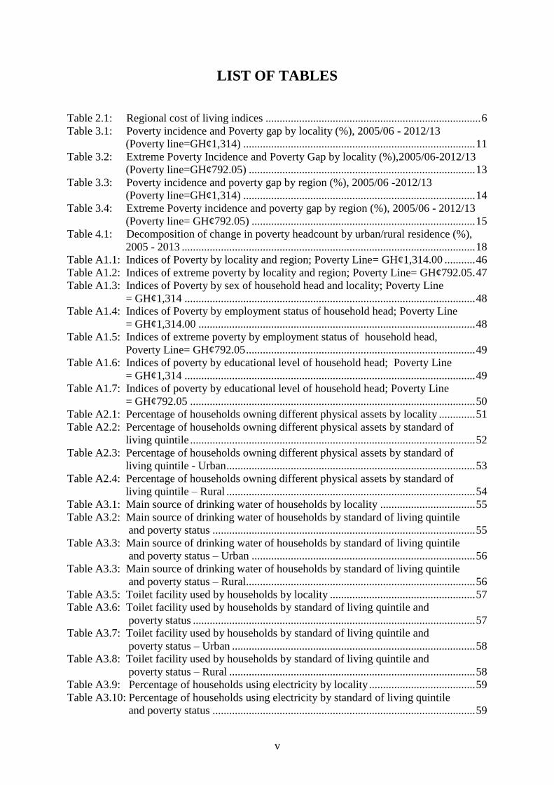
LIST OF TABLES
Table 2.1: Regional cost of living indices ............................................................................. 6 Table 3.1: Poverty incidence and Poverty gap by locality (%), 2005/06 - 2012/13 (Poverty line=GH¢1,314) ................................................................................... 11 Table 3.2: Extreme Poverty Incidence and Poverty Gap by locality (%),2005/06-2012/13 (Poverty line=GH¢792.05) ................................................................................. 13
Table 3.3: Poverty incidence and poverty gap by region (%), 2005/06 -2012/13 (Poverty line=GH¢1,314) ................................................................................... 14 Table 3.4: Extreme Poverty incidence and poverty gap by region (%), 2005/06 - 2012/13
(Poverty line= GH¢792.05) ................................................................................ 15 Table 4.1: Decomposition of change in poverty headcount by urban/rural residence (%), 2005 - 2013 ......................................................................................................... 18 Table A1.1: Indices of Poverty by locality and region; Poverty Line= GH¢1,314.00 ........... 46
Table A1.2: Indices of extreme poverty by locality and region; Poverty Line= GH¢792.05. 47 Table A1.3: Indices of Poverty by sex of household head and locality; Poverty Line = GH¢1,314 ........................................................................................................ 48 Table A1.4: Indices of Poverty by employment status of household head; Poverty Line
= GH¢1,314.00 ................................................................................................... 48 Table A1.5: Indices of extreme poverty by employment status of household head, Poverty Line= GH¢792.05 .................................................................................. 49
Table A1.6: Indices of poverty by educational level of household head; Poverty Line
= GH¢1,314 ........................................................................................................ 49 Table A1.7: Indices of poverty by educational level of household head; Poverty Line = GH¢792.05 ...................................................................................................... 50
Table A2.1: Percentage of households owning different physical assets by locality ............. 51 Table A2.2: Percentage of households owning different physical assets by standard of
living quintile ...................................................................................................... 52 Table A2.3: Percentage of households owning different physical assets by standard of living quintile - Urban ......................................................................................... 53
Table A2.4: Percentage of households owning different physical assets by standard of living quintile – Rural ......................................................................................... 54
Table A3.1: Main source of drinking water of households by locality .................................. 55 Table A3.2: Main source of drinking water of households by standard of living quintile
and poverty status .............................................................................................. 55 Table A3.3: Main source of drinking water of households by standard of living quintile and poverty status – Urban ................................................................................ 56 Table A3.3: Main source of drinking water of households by standard of living quintile and poverty status – Rural.................................................................................. 56
Table A3.5: Toilet facility used by households by locality .................................................... 57 Table A3.6: Toilet facility used by households by standard of living quintile and poverty status ..................................................................................................... 57 Table A3.7: Toilet facility used by households by standard of living quintile and
poverty status – Urban ....................................................................................... 58
Table A3.8: Toilet facility used by households by standard of living quintile and poverty status – Rural ........................................................................................ 58 Table A3.9: Percentage of households using electricity by locality ...................................... 59 Table A3.10: Percentage of households using electricity by standard of living quintile and poverty status .............................................................................................. 59

vi
Table A4.1: Type of health personnel consulted by ill or injured individuals by locality ..... 60 Table A4.2: Type of health personnel consulted by ill or injured individuals by standard of living quintile and poverty status................................................................... 60 Table A4.3: Type of health personnel consulted by ill or injured individuals by standard of living quintile and poverty status - Urban ..................................................... 61
Table A4.4: Type of health personnel consulted by ill or injured individuals by standard of living quintile and poverty status - Rural ...................................................... 61 Table A4.5: Where consultation took place for ill or injured individuals by locality ............ 62 Table A4.6: Where consultation took place for ill or injured individuals by standard of living quintile and poverty status ....................................................................... 62
Table A4.7: Where consultation took place for ill or injured individuals by standard of
living quintile and poverty status – Urban ......................................................... 63 Table A4.8: Where consultation took place for ill or injured individuals by standard of
living quintile and poverty status - Rural ........................................................... 63 Table A4.9: Net enrolment in primary school, by locality, gender and standard of living quintile ..................................................................................................... 64 Table A4.10: Net enrolment in JSS/JHS, by locality, sex poverty status and standard of living quintile ..................................................................................................... 65
Table A4.11: Net enrolment in secondary school, by locality, sex, poverty status and
standard of living quintile .................................................................................. 66 Table A5.1: Indices of Poverty by locality using the old poverty line: GH¢370.89 ............. 67 Table A5.2: Indices of Poverty by locality using the old poverty line: GH¢288.47 ............. 68
Table A6.1: Main macroeconomic statistics and indicators, 2005-2013 ............................... 69
Table A8.1: Estimation of total household consumption expenditure from the GLSS 3-5 and GLSS6 surveys ............................................................................................ 74 Table A8.2: Recommended energy intakes ........................................................................... 75

vii
LIST OF FIGURES
Figure 1.1: Annual GDP growth rates (%), 2005 -2013 ........................................................... 1 Figure 1.2: Sectoral distribution of GDP (%), 2005-2013 ........................................................ 2 Figure 1.3: Average annual per capita growth (%) for selected countries in Africa and Asia,
2005-2012 .............................................................................................................. 2 Figure 1.4: Combined, food and non-food inflation rates (%), 2005-2013 .............................. 3 Figure 1.5: Total, recurrent and capital Government budget expenditure (million Ghana Cedis) ............................................................................................ 4 Figure 3.1: Poverty incidence by locality (Poverty line= GH ¢1,314) ................................... 11
Figure 3.2: Extreme poverty incidence by locality (Poverty line=GH¢ 792.05) .................... 13
Figure 3.3: Poverty incidence by region (Poverty line=GH¢1,314) ....................................... 15 Figure 3.4: Extreme poverty incidence by locality (Poverty line=GH¢792.05) ................... 16
Figure 3.5: Extreme poverty incidence by region (Poverty line=GH¢792.05) ..................... 16 Figure 4.1: Poverty Incidence by employment status of household, 2005/05-2012/13 (Poverty line=GH¢1,314) .................................................................................... 19 Figure 4.2: Poverty incidence by sex of household heads, 2005/06-2012/13 (Poverty line=GH¢1,314) .................................................................................... 19
Figure 4.3: Poverty incidence by education level of household’s head (Poverty line
= GH¢1,314) ........................................................................................................ 20 Figure 4.4: Poverty gap by household head’s education level, (Poverty line= GH¢1,314) ... 20
Figure 4.5: Inequality by locality: Gini coefficient, 2005/06-2012/13 ................................... 22
Figure 4.6: Inequality by region: Gini coefficient, 2005/06 – 2012/13 .................................. 22
Figure 4.7: Growth incidence curve for Ghana, 2005-- 2013 ................................................. 24 Figure 4.8: Growth incidence curve for urban Ghana, 2005 - 2013 ....................................... 24
Figure 4.9: Growth incidence curve for rural Ghana, 2005 - 2013 ......................................... 25 Figure 5.1: Percentage of urban households owning different household assets, 1998/99-2012/13 .................................................................................................. 27
Figure 5.2: Percentage of rural households owning different household assets, 1998/99-2012/13 .................................................................................................. 27
Figure 5.3: Percentage of urban households owning different transportation assets, 1998/99-2012/13 ................................................................................................... 28 Figure 5.4: Percentage of rural households owning different transportation assets,
1998/99-2012/13 ................................................................................................... 28 Figure 5.5: Percentage of households owning a refrigerator by locality and quintile, 1998/99-2012/13 ................................................................................................... 29
Figure 5.6: Percentage of households owning a television set by locality and quintile, 1998/99-2012/13 ................................................................................................... 29 Figure 6.1: Percentage of households using potable water by locality and standard of living quintile, 1998/99-2012/13 ......................................................................... 32 Figure 6.2: Percentage of households using flush or KVIP toilet by locality and standard
of living quintile, 1998/99-2012/13 ..................................................................... 33 Figure 6.3: Percentage of households using electricity by locality and standard of living quintile, 1998/99-2012/13 .................................................................................... 33
Figure 7.1: Percentage of ill or injured individuals that consulted a doctor by locality and standard of living quintile, 1998/99-2012/13....................................................... 35 Figure 7.2: Percentage of ill or injured individuals that consulted a pharmacist/ chemical seller by locality and standard of living quintile, 1998/99-2012/13 .................... 35

viii
Figure 7.3: Percentage of ill or injured individuals that went to a hospital by locality and standard of living quintile, 1998/99-2012/13 ............................................... 36 Figure 7.4: Percentage of ill or injured individuals that went to a health facility by locality and standard of living quintile, 1998/99-2012-13 ............................................... 36 Figure 7.5: Net primary school attendance ratio by sex and locality, 2005/06-2012/13 ....... 37
Figure 7.6: Net primary school attendance rate by sex and quintile, 2005/06-2012/13 ........ 38 Figure 7.7: Gross primary school attendance rate by sex and locality, 2005/06-2012/13 ..... 39 Figure 7.8: Net JHS school attendance rate by sex and locality, 2005/06-2012/13 .............. 39 Figure 7.9: Net JHS school attendance rate by sex and quintile, 2005/06-2012/13 .............. 40 Figure 7.10: Gross JHS attendance rate by sex and locality, 2005/06-2012/13 ...................... 40
Figure 7.11: Gross JHS school attendance rate by sex and quintile, 2005/06-2012/13........... 41
Figure 7.12: Net SHS school attendance rate by sex and locality, 2005/06-2012/13 .............. 41 Figure 7.13: Net SHS school attendance rate by sex and quintile, 2005/06-2012/13 ............. 42
Figure 7.14: Gross SSS school attendance rate by sex and quintile, 2005/06-2012/13........... 42

ix
ACRONYMS AND ABBREVIATIONS
CPI Consumer Price Index
GAMA Greater Accra Metropolitan Area
GLSS Ghana Living Standard Survey
GDP Gross Domestic Product
GIC Growth Incidence Curve
GAR Gross Attendance Rate
JHS Junior High School
KVIP Kumasi Ventilated Improved Pit
LEAP Livelihood Empowerment Against Poverty
MSMEs Medium Small and Micro Enterprises
NAR Net Attendance Rate
MDG Millennium Development Goal
TV Television
SHS Senior High School
WDI-WB World Development Indicators-World Bank
WHO World Health Organization

x
EXECUTIVE SUMMARY
Introduction
The Ghana Living Standards Survey is a nationally representative sample survey undertaken
to measure the living conditions and well-being of the population. The survey also provides
the required data for examining the poverty profile of households and the decomposition
between different groupings: urban/rural, locality, region and socio-economic status.
Since 2005, the Ghanaian economy has undergone several changes and available data show
that the Gross Domestic Product (GDP) recorded a growth ranging from 4.5 percent and 15.0
percent between 2005 and 2013. The country also attained a lower-middle income status
during the period. Several social intervention programmes, including the Livelihood
Empowerment Against Poverty (LEAP), Capitation Grant and School Feeding Programme,
have been implemented with the aim of alleviating poverty among the vulnerable population.
Poverty has many dimensions and is characterized by low income, malnutrition, ill-health,
illiteracy and insecurity, among others. The impact of the different factors could combine to
keep households, and sometimes whole communities, in abject poverty. In order to address
these, reliable information is required to develop and implement policies that would impact
the lives of the poor and vulnerable.
This report is based on the sixth round of the Ghana Living Standards Survey (GLSS6)
conducted in 2012/2013. Previous rounds of the survey have been conducted in 1987/88,
1988/89, 1998/99 and 2005/2003. The report does not seek to compare the results of the
current survey to previous ones due to changes in the Consumer Price Index (CPI) basket,
introduction of new consumer items onto the market and changes in household consumption.
The report therefore provides a profile of poverty computed from the GLSS6 data and
attempts to examine changes in the past 7 years by adjusting welfare levels in 2005/06 using
the 2012/13 consumption basket and price levels.
Economic Context
The annual GDP growth rates recorded in Ghana for the period 2005 to 2013 ranged from 4.0
percent to 15.0 percent with the lowest growth rate recorded in 2009 and the highest in 2011.
The average annual growth rate recorded for the same period was 7.8 percent. From 2010 to
2013, the country experienced an annual average GDP growth rate of 9.7 percent, with per
capita income rising above GH¢1,000.00 in 2007, which made Ghana a low-middle income
country. The country's average annual growth rate of GDP per capita in constant 2006 prices
was 5.2 percent for the period 2005-2012.
Regarding inflation, the non-food inflation rate has mainly been responsible for the high
inflation rate in Ghana. The average annual non-food inflation rate for the period 2005-2013
was 14.9 percent and has been consistently higher than the average annual food inflation rate
of 9.5 percent.
Over the period 2005 to 2013, Ghana’s Balance of Payments averaged a deficit of US$0.08
billion with the highest deficit of US$1.46 billion recorded in 2010 while the lowest
(US$0.08) occurred in 2005. The size of government’s expenditure in nominal terms, over
the past eight years, increased from 2,970.62 million Ghana Cedis in 2005 to 26,277.17
million Ghana Cedis in 2013

xi
Consumption Poverty, Methodology and Measurement
The Ghana Living Standards Survey collects sufficient information to estimate total
consumption of each household. This covers consumption of both food and non-food items
(including housing).
In using measures of household consumption to compare living standards across geographical
areas, account was taken of the variations in the cost of living across regions, as well as
differences in household size and composition (children & adults and males & females).
The measure of the standard of living is based on household consumption expenditure,
covering food and non-food items, including housing. The regional cost of living index is
based on regional monthly food and non-food CPI weighted by region and urban-rural shares.
Greater Accra is more expensive than other regions regarding food items whereas non-food
items are more expensive outside Accra except in the three Northern regions.
Two key adjustments has been made to the household consumption construction based on
GLSS6 to compensate for the changes in consumption patterns. These are the inclusion of the
user values of VCD/DVD/mp4 player/iPad, vacuum cleaner, rice cooker, toaster, electric
kettle, water heater, tablet PC and mobile phone; and relaxing the cleaning procedure,
replacing the values of expenditure items above 5 standard deviations with the mean for that
locality (3 standard deviations was used in the previous surveys).
Profile of Consumption Poverty
This section looks at analysing Ghana’s poverty profile using the most recent surveys. The
survey results show that about a quarter of Ghanaians are poor whilst under a tenth of the
population are in extreme poverty. In spite of the fact that the level of extreme poverty is
relatively low, it is concentrated in Rural Savannah, with more than a quarter of the people
fallen into this category. Overall, the dynamics of poverty in Ghana over the 7-year period
indicate that poverty is still very much a rural phenomenon.
Five out of the ten regions had their rates of poverty incidence lower than the national
average of 24.2 percent while the remaining half had rates higher than the national average.
Greater Accra is the least poor region and the Upper West the poorest overall. Though most
regions show a reduction in poverty incidence since 2005/06, the pattern of poverty by region
remains the same.
Covariate Analysis
The data reveal that household heads who are farmers are not just the poorest in Ghana, but
they also contribute the most to Ghana’s poverty. Household heads engaged as private
employees and self-employed in non-agricultural sectors are less likely to be poor than those
engaged in the agricultural sector. Over the period, public sector earners have, as a result of
the public sector wage rationalization policy implemented in 2009, experienced a reduction in
poverty.
In general, female-headed households appear to be better off than male-headed households in
terms of poverty incidence. Households with uneducated household heads are also found to
be the poorest in Ghana and contribute the most to Ghana’s poverty incidence.
From the data, welfare distribution is more disproportionate in Ghana now than in 2005/06
which indicates an increasing inequality as measured by the Gini coefficient. While some
regions showed improvement in terms of the equality in the distribution of welfare, other
xii
regions such as Volta and Upper West experienced worsening welfare distribution between
2005/06 and 2012/13. Generally, those in the lower income brackets and the population
above the 60th
percentile benefited the most from the growth in consumption.
Household Assets
Information was collected on household assets over the survey period. The proportions of
households owning most of the durable goods covered in the surveys have shown large
increases between 1998/99 and 2005/2006, and further increases in 2012/13. Both urban and
rural areas experienced these increases but which have often been higher for wealthier
groups, with greater disparity among urban households. Ownership of durable goods remains
much lower in rural areas than urban areas, even among households of similar overall living
standards
Access to Services
In terms of access to services, the data show that there have been major improvements over
the fifteen-year period in the number of households obtaining their drinking water from an
improved source, using adequate toilet facilities and having access to electricity. Rural areas
and poorer urban households benefited most from the increases in the use of adequate
drinking water sources. Rural households again experienced more marked improvements in
access to adequate toilet facilities.
Human Development
Information from the survey show that the period 2005/06 to 2012/13 witnessed increased
rates of access to a range of health services. Nevertheless, disparities remain between urban
and rural areas and between quintile groups within those areas. From the data, individuals are
more likely now to consult doctors and visit health facilities compared to the 1998/99 and
2005/06 period. Persons who consult pharmacists or chemical sellers when ill or injured has
decreased while the percentage of individuals ill or injured who did not consult any health
practitioner has declined.
Regarding education, school attendance rates in primary, JHS and SHS have improved over
the period 2005/06 to 2012/13 with the savannah areas still reporting the lowest school
attendance rates. Increases in net school attendance rates at the JHS level have been much
higher for girls than boys, but are still below those for boys.

1
CHAPTER ONE
THE ECONOMIC CONTEXT
1.1 Gross Domestic Product (GDP), 2005-2013
The annual GDP growth rates recorded in Ghana for the period 2005 to 2013 ranged from 4.0
percent to 15.0 percent; the lowest growth rate was recorded in 2009 and the highest in 2011.
The average annual growth rate for the same period was 7.8 percent (Figure 1.1). From 2010
to 2013, however, the country experienced an annual average GDP growth rate of 9.7
percent, with per capita income rising above GH¢1000.00 in 2007, making Ghana a low-
middle income country. Currently, Ghana is one of the fastest growing economies in the
world.
Figure 1.1: Annual GDP growth rates (%), 2005 -2013
Figure 1.2 reflects the sectoral distribution of the GDP for the Agriculture, Manufacturing,
Other industry (without manufacturing), and Services sectors. The graph shows that the
recent growth has been significantly driven by the Services sector and other industry except
Manufacturing (e.g., mineral exports, especially crude oil since 2011), Utilities and
Construction while the contributions of the Agriculture and Manufacturing sectors have
dwindled. The Manufacturing sector, whose share of output has greatly reduced since 2005,
holds the key to sustained growth in the economy since it is the most versatile job creation
sector.
Available data suggests that the GDP per capita in constant 2006 prices grew from 824.0
million Ghana Cedis in 2005 to 1,173.0 million Ghana Cedis in 2012 and further to 1,227.7
million Ghana Cedis in 2013. This puts the average annual growth rate of GDP per capita in
constant 2006 prices at 5.2 percent for the period 2005-2012.
5.9 6.2 6.5 8.4
4.0
8.0
15.0
8.8 7.1 7.8
0
5
10
15
20
20
05
20
06
20
07
20
08
20
09
20
10
20
11
20
12
20
13
Ave
rage
Gro
wth
Ghana Statistical Service (GSS)
%

2
Figure 1.2: Sectoral distribution of GDP (%), 2005-2013
Figure 1.3 compares Ghana’s average annual GDP per capita between 2005 and 2012 to 49
other countries (45 in Africa and 4 from Asia including Indonesia, Vietnam, India and
Mongolia). The results indicate that Ghana’s average per capita income growth of 5.2 percent
was the seventh highest during the period.
Figure 1.3: Average annual per capita growth (%) for selected countries in Africa
and Asia, 2005-2012
Source: World Development Indicators-World Bank, different editions
42 30 29 31 32 30 25 23 22
10
10 9 8 7 7 7 6 6
17
11 12 12 12 12 19 22 23
31 49 50 49 49 51 49 48 49
0
20
40
60
80
100
2005 2006 2007 2008 2009 2010 2011 2012 2013
Services etc.
Industry excludingmanufacturing
Manufacturing
Agriculture
2.2
5.4
-4.0 -2.0 0.0 2.0 4.0 6.0 8.0 10.0
EritreaComoros
ZimbabweGuinea-Bissau
MadagascarSwaziland
GuineaGambia, TheCote d'Ivoire
MalawiSenegal
Equatorial GuineaCameroon
BurundiBenin
GabonMaliTogoChadNiger
Congo, Rep.South Africa
KenyaGhana 1998-2005
MauritaniaBurkina Faso
NamibiaCongo, Dem. Rep.
SudanBotswana
ZambiaMauritiusTanzania
SeychellesUgandaLesothoNigeria
MozambiqueIndonesia
Sierra LeoneCentral African Republic
VietnamRwanda
Ghana 2005-2012Cabo Verde
IndiaAngola
EthiopiaMongolia
Liberia
3
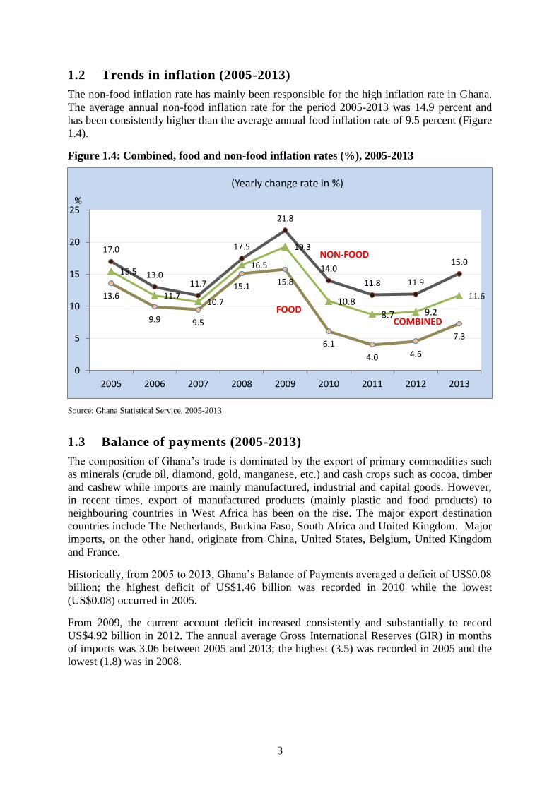
1.2 Trends in inflation (2005-2013)
The non-food inflation rate has mainly been responsible for the high inflation rate in Ghana.
The average annual non-food inflation rate for the period 2005-2013 was 14.9 percent and
has been consistently higher than the average annual food inflation rate of 9.5 percent (Figure
1.4).
Figure 1.4: Combined, food and non-food inflation rates (%), 2005-2013
Source: Ghana Statistical Service, 2005-2013
1.3 Balance of payments (2005-2013)
The composition of Ghana’s trade is dominated by the export of primary commodities such
as minerals (crude oil, diamond, gold, manganese, etc.) and cash crops such as cocoa, timber
and cashew while imports are mainly manufactured, industrial and capital goods. However,
in recent times, export of manufactured products (mainly plastic and food products) to
neighbouring countries in West Africa has been on the rise. The major export destination
countries include The Netherlands, Burkina Faso, South Africa and United Kingdom. Major
imports, on the other hand, originate from China, United States, Belgium, United Kingdom
and France.
Historically, from 2005 to 2013, Ghana’s Balance of Payments averaged a deficit of US$0.08
billion; the highest deficit of US$1.46 billion was recorded in 2010 while the lowest
(US$0.08) occurred in 2005.
From 2009, the current account deficit increased consistently and substantially to record
US$4.92 billion in 2012. The annual average Gross International Reserves (GIR) in months
of imports was 3.06 between 2005 and 2013; the highest (3.5) was recorded in 2005 and the
lowest (1.8) was in 2008.
13.6
9.9 9.5
15.1 15.8
6.1
4.0 4.6
7.3
17.0
13.0 11.7
17.5
21.8
14.0
11.8 11.9
15.0 15.5
11.7 10.7
16.5
19.3
10.8
8.7 9.2
11.6
0
5
10
15
20
25
2005 2006 2007 2008 2009 2010 2011 2012 2013
(Yearly change rate in %)
%
FOOD COMBINED
NON-FOOD

4
1.4 Public expenditures (2005-2013)
Figure 1.5 shows that the size of government’s expenditure in nominal terms, over the past
eight years, increased from 2,970.62 million Ghana cedis in 2005 to 26,277.17 million Ghana
cedis in 2013. The Figure further displays government’s spending on recurrent and capital
goods over time and illustrates the growing importance of recurrent expenditure vis-a-vis
capital expenditure which can help sustain the current economic growth trajectory.
Figure 1.5: Total, recurrent and capital Government budget expenditure
(million Ghana Cedis)
1.5 Social interventions
In the past two decades, several social intervention programmes, including the Livelihood
Empowerment Against Poverty (LEAP), Capitation Grant, School Feeding Programme, free
distribution of school uniforms, exercise books and textbooks, elimination of schools under
trees, have been implemented with the aim of alleviating poverty among the vulnerable
population in Ghana. Other projects aimed at improving health care delivery have also been
implemented. These include the establishment of Community-based Health Planning Services
(CHPS), national immunization against polio and indoor residual spraying against malaria
carrying mosquitoes.
1.6 Summary
Since the last Ghana Living Standards Survey (GLSS5), the Ghanaian economy has
continued to benefit from strong economic growth leading to the achievement of lower
middle income status. However, it remains to be seen whether this growth has benefitted all
sections of society, including the poorest.

5
CHAPTER TWO
CONSUMPTION POVERTY, METHODOLOGY AND
MEASUREMENT
2.1 Introduction
A report on consumption poverty is specifically concerned with the population whose
standard of living falls below a defined consumption basket, represented by a poverty line. In
achieving this, two issues need to be addressed:
The measurement of the standard of living; and
The determination of a poverty line.
In this study, following common practice in many countries, a consumption-based standard of
living measure is used. The poverty line is set at that level of the minimum consumption
requirement.
2.2 Data sources
The main data source for this report is the sixth round of the Ghana Living Standards Survey
(GLSS). The GLSS is a multi-purpose household survey which collects information on many
different dimensions of living conditions, including education, health, employment and
household expenditure on food and non-food items.
Six rounds of data have been collected starting in 1987/88 but in this report, we focus on the
most recent rounds of GLSS, 2005/06 and 2012/13. The questionnaires used for all these
rounds were almost identical, meaning that their results can be directly compared. By
contrast, the first two rounds were based on different questionnaires, making comparison with
the later rounds more difficult.
GLSS collects sufficient information to estimate total consumption of each household. This
covers consumption of both food and non-food items (including housing). Food and non-
food consumption commodities may be explicitly purchased by households, or acquired
through other means (e.g., as output of own production activities, payment for work done in
the form of commodities, or from transfers from other households). The household
consumption measure takes into account all these sources in the different modules of the
questionnaires (Appendix 8, Table A8.1).
2.3 Construction of the standard of living measure
In using measures of household consumption to compare living standards across geographical
areas, it is necessary to take into account variations in the cost of living across regions, as
well as differences in household size and composition (children & adults and males &
females). The composition is taken to reflect the different calorie requirements.
As in the previous poverty profile report (GSS, 2007), the measure of the standard of living is
based on household consumption expenditure, covering food and non-food items (including
housing). The regional cost of living index is based on regional monthly food and non-food
CPI weighted by region and urban-rural shares.

6
Table 2.1 shows the regional cost of living indices with regions compared to Greater Accra as
the base. Accra, the capital city of Ghana, is located in the Greater Accra region. For food
items, Greater Accra is more expensive than other regions; whereas non-food items are more
expensive outside Accra except in the three Northern regions.
Table 2.1: Regional cost of living indices
Region Price index Food Non-food
Western 1.0260
0.9977
1.0566
Central 0.9883
0.9596
1.0276
Greater Accra 1.0000
1.0000
1.0000
Volta 0.9998
0.9576
1.0591
Eastern 0.9757
0.9574
1.0052
Ashanti 0.9963
0.9161
1.0792
Brong Ahafo 0.9792
0.9534
1.0140
Northern 0.9799
0.9811
0.9920
Upper East 0.9366
0.9082
0.9952
Upper West 0.9591 0.9399 0.9919
Source: Computed from the Ghana Living Standards Survey, 2012/13 and monthly regional CPI
The overall cost of living index also allows for variation in prices over time within the survey
period, based on the monthly regional Consumer Price Index. The use of regional specific
CPIs allows us to take into account adjustment in relative spatial prices. In this way, each
household’s consumption expenditure is expressed in the constant prices of Greater Accra in
January 2013.
The number of equivalent adults is calculated based on the composition of the household,
using a calorie-based scale from the 10th
Edition of the National Research Council’s
Recommended Dietary Allowances (Washington D.C.: National Academy Press, 1989). This
scale has commonly been applied in nutritional studies in Ghana. The “Equivalent adults”
measure recognizes, for example, that the consumption requirements of babies or young
children are less than those of adults. The scale is based on age and gender specific calorie
requirements, and is given in Table A8.2 (Appendix 8).
Each individual is represented as having the standard of living of the household to which they
belong. It is not possible to allow for intra-household variations in living standards using the
consumption measure, though some other indicators considered later do take account of intra-
household variations.
2.4 Rebasing of the standard of living measurement
In this poverty profile report, the standard of living is measured per adult equivalent
consumption, derived by dividing the total household consumption with the number of adult
equivalents in the household. In order to measure standard of living consistently over time,
the methodology of constructing household consumption must be consistent. However,
periodic adjustments of consumption aggregates are needed to reflect the changes in the
consumption pattern. Such an adjustment is needed between GLSS3-GLSS5 (1991-2005) and
GLSS6 (2013) because new consumer goods have entered the consumption basket of
Ghanaian households that were non-existent in previous surveys. Due to these changes in
consumption patterns, we have made two adjustments to the household consumption
construction based on GLSS6:
7
1. Inclusion of the user values of VCD/DVD/mp4 player/iPad, vacuum cleaner, rice
cooker, toaster, electric kettle, water heater, tablet PC and mobile phone. 1
2. Relaxed the cleaning procedure, replacing the values of expenditure items above 5
standard deviations with the mean for that locality (3 standard deviations was used
in the previous surveys).
2.5 Rebasing the consumption basket and construction of the
Poverty Line
Following the GLSS 5 methodology, the consumption expenditure for a minimum food
basket providing 2,900 calories per adult equivalent per day was calculated. This is the
extreme poverty line, which means that a household’s total consumption expenditure is not
even adequate to meet this minimum calorie requirement. An additional expenditure on non-
food items was added to the extreme poverty line to produce the absolute poverty line (for
methodology see Box1).
As consumption patterns change, it is necessary to update the minimum consumption basket
deemed adequate to provide an acceptable living standard in the current Ghanaian society.
For example, expenditure on mobile phones and other small electronic devices were rare in
2005, but have become more prevalent in today’s society.
2.6 Summary
In summary, the standard of living for each individual is measured as the total consumption
expenditure per equivalent adult, of the household to which he or she belongs, expressed in
constant prices of Greater Accra in January 2013.
Two nutritionally-based poverty lines are derived from this procedure:
A lower poverty line of 792.05 Ghana cedis per adult per year: this focuses on what
is needed to meet the nutritional requirements of household members. Individuals
whose total expenditure falls below this line are considered to be in extreme poverty,
since even if they allocated their entire budget to food, they would not be able to meet
their minimum nutrition requirements (if they consume the average consumption
basket). This line is 27.1 percent of the mean consumption level in 2012/13.
An upper poverty line of 1314.00 Ghana cedis per adult per year: this incorporates
both essential food and non-food consumption. Individuals consuming above this
level can be considered able to purchase enough food to meet their nutritional
requirements and their basic non-food needs. This line is 44.9 percent of the mean
consumption level in 2012/13.
1 User value is calculated as 20 percent of the selling value of consumer items.
8
Box 1: Setting a poverty line for Ghana
Setting an absolute poverty line for a country is not a precise scientific exercise. Though an
absolute poverty line can be defined as that value of consumption necessary to satisfy
minimum subsistence needs, difficulties arise in specifying these minimum subsistence needs
as well as the most appropriate way of attaining them. In the case of food consumption,
nutritional requirements can be used as a guide. In practice, this is often restricted to calorie
requirements, but even then, there are difficult issues about which food basket to choose and
the expenditure required for the minimum non-food consumption basket.
In practice, the minimum expenditure to meet adequate calorie requirements is generally used
as the basis for an estimated poverty line (referred to as the extreme poverty line), based on
the information about quantities of foods consumed by households and the calorie contents of
these foods.
Following the GLSS6, it has become necessary to recalculate new poverty lines as a result of
changes in the consumption basket of the Ghanaian population. Items such as DVD/VCD,
MP3/MP4 players, vacuum cleaner, rice cooker, mobile phone, tablet PCs, etc., have been
included in the new basket.
In line with international practice, we calculate the average expenditure of the food
consumption basket for the bottom 50 percent of individuals ranked by the standard of living
measure, and derive the amount of calories in this basket. The calorie price is then calculated
by dividing the adult equivalent expenditure of the food basket by the amount of adult
equivalent calories provided by the basket. This calorie price is representative of the price
paid by a typical household in the bottom 50 percent. This price is then multiplied by 2900
calories which was used to calculate the poverty lines for the 2012/13 survey.
Following common practice in other developing countries, expenditure on non-food
consumption is added to the extreme poverty line calculated above. This non-food basket is
determined by those whose total food expenditure is about the level of the extreme poverty
line (10 percent individuals below and above the line). This is based on Engel’s law which
states that the share of food expenditure decreases as household income/expenditure
increases. By selecting the population whose food consumption is around the extreme
poverty line, their non-food expenditure is used as the benchmark for estimating the absolute
poverty line.
The methodology used produced an extreme poverty line of 792.05 Ghana cedis and an
absolute poverty line of 1,314.00 Ghana cedis per equivalent adult per year in the January
2013 prices of Greater Accra Region. In dollar terms, the absolute poverty line is equivalent
to about $1.83 per day ($1.10 for the extreme poverty line). The absolute poverty line
indicates the minimum living standard in Ghana while the extreme poverty line indicates that
even if a household spends their entire budget on food, they still would not meet the
minimum calorie requirement.
9
CHAPTER THREE
PROFILE OF CONSUMPTION POVERTY
3.1 Introduction
Overtime, Ghana’s poverty analysis has focused on consumption poverty which has classified
the poor as those who lack command over basic consumption needs, including food and non-
food components. In estimating who is poor and who is non-poor, the expenditure of a
minimum consumption basket required by an individual to fulfill his or her basic food and
non-food needs was calculated. This expenditure is referred to as the poverty line or absolute
poverty line. In addition to the poverty line, an extreme poverty line is also commonly
estimated. This line indicates the expenditure required for a minimum food consumption
basket that can provide adequate calories to a household. A household living below the
extreme poverty line cannot afford this adequate calorie requirement even if it were to spend
all its budget on food.
In the literature, applying these poverty lines to the distribution of the standard of living
measure usually results in estimating several poverty indicators when measuring poverty.
This report focuses on analysing Ghana’s poverty profile using the most recent surveys.
3.2 Poverty incidence and poverty gap
The focus of this section is the analysis of two poverty indicators, poverty incidence (P0) and
poverty gap index (P1), which were estimated by applying the two above-mentioned poverty
lines to the distribution of the standard of living measure.
In theory, these two indicators are defined as:
1. The headcount index (P0), also called the poverty incidence. This measures the
proportion of the population that is poor. It is popular because it is easy to
understand and measure but it does not indicate how poor the poor are.
2. The poverty gap index (P1) measures the intensity of poverty in a country, which is the
average ratio of the gap to which individuals fall below the poverty line (for non-poor
the gap is counted as zero). The sum of these poverty measures gives the minimum
cost of eliminating poverty, if transfers were perfectly targeted. The measure does not
reflect changes in inequality among the poor, but adds up the extent to which
individuals on average fall below the poverty line, and expresses it as a percentage of
the poverty line.
The objective of this section is to examine the poverty situation in 2012/13 in particular and
inequality in the welfare distribution since the last poverty estimates were produced
(2005/06) in a bid to examine the patterns of poverty over the 7-year period. These patterns
are considered across geographical location, administrative regions and various
socioeconomic groups.
Considering the upper poverty line of GH¢1,314, the proportion of the population defined as
poor is 24.2 percent in 2012/2013, with a poverty gap index of 7.8 percent (in other words,
the mean income of the poor falls below the poverty line by 7.8%). These percentages
indicate that about 6.4 million people in Ghana are poor.

10
Based on the new poverty line for 2012/13, the welfare levels for 2005/06 were adjusted with
a deflator of 3.3 for non-food and 2.9 for food; these were estimated over the 7-year period
using the consumer price index for the period under consideration. The revised welfare levels
for 2005/06 indicate that overall poverty incidence for 2005/06 was 31.9 percent with a
poverty gap of 11.0 percent. That is, if Ghanaians were consuming the current basket of items
in 2005/06, poverty levels for Ghana for 2005/06 would have been 31.9 percent (Appendix
5).
The results from the GLSS5 and GLSS6 surveys indicate that given a poverty line of
GH¢1,314, poverty reduced by 7.7 percentage points over the seven-year period (2005/2006
to 2012/13). Similarly, the 2005/06 report on poverty trends in Ghana indicates that in
1991/92, the poverty rate was 51.7 percent. Given that the rate for 1991/92 is not any
different from the rate in 1990, then unless the unexpected happens in the next two years in
the Ghanaian economy which may result in a slippage, the MDG 1 target, which seeks to
halve poverty by 2015 from the rate in 1991/92 (51.7%) will inevitably be met by 2015, since
the current (2013) poverty rate is even slightly less than half the rate recorded in 1991/92
(Table 3.1, Figure 3.1 and Table A1.1).
The contribution to poverty incidence varied across various demographic groupings. In
2012/13, the rural population comprised 50 percent of the population of Ghana, yet it
accounts for 78 percent of those in poverty. This is in line with previous poverty profile
reports (GSS 1998/99 and 2005/06) where above 80 percent of the total population living
below the poverty line in Ghana were living in the rural areas (Table 3.1 and Table A1.1).
Among rural localities where poverty is prominent, the poverty incidence is much higher
among those living in rural savannah. In the 12 month period 2012/13, the contribution to
poverty incidence in rural savannah is found to be higher than in rural coastal and forest
combined. Notably, rural savannah contributes more than 40 percent to the overall poverty in
Ghana. This phenomenon confirms previous poverty reports which indicate that the poverty
decline in Ghana (from 1998/99 to 2005/06) has not been evenly distributed geographically
(Table 3.1 and Table A1.1).
Greater Accra (GAMA) which includes the capital of Ghana recorded the lowest poverty
incidence of 3.5 percent among all the geographical areas. The 2010 Population and Housing
Census results indicate that of all the measurements of migration effectiveness, Greater Accra
Region had a net gain of 66.4 percent of internal migrants. Most of these internal migrants are
likely to have come to Accra to seek greener pastures, but they virtually end up as self-
employed in non-agricultural activities, such as the service sectors to engage in petty trading.
Juxtaposing the above with results from Figure 4.1 (Chapter 4) which reports on poverty
incidence by employment status of household head, it is observed that a large proportion of
individuals engaging in service sector activities are above the poverty line. One can therefore
infer that households engaged in the service sector contributed to the low rate of poverty
reported in Greater Accra. Indeed, the increasing number of microfinance institutions
providing loans for activities in this sector may have contributed to this improvement in
welfare, with Accra being the greatest beneficiary. According to the quarterly report of the
Bank of Ghana, the provisional list shows that by March 2013, 61 percent of the nationwide
microfinance institutions were located in Accra. This is an indication that the capital base of
the self-employed without employees are improved over time, and given that the location of
the establishment of the microfinance institutions are demand driven, many MSMEs would
have access to credit facilities which may eventually improve the welfare of people living in
Accra.
11
The information considered so far only relate to the numbers classified as poor, without
considering the extent of poverty. The poverty depth, the proportion by which the average
consumption level of poor households in Ghana falls below the poverty line, gives some
indication of just how intense poverty has been in Ghana. This ratio (dividing poverty gap by
poverty incidence) indicates that on average the poor population in Ghana lived 32 percent
below the poverty line of GH¢1,314. Again, relative to the poverty line, the rural population
accounts for more than eighty percent of the poverty gap. (Table 3.1, Figure 3.1, and Table
A1.1).
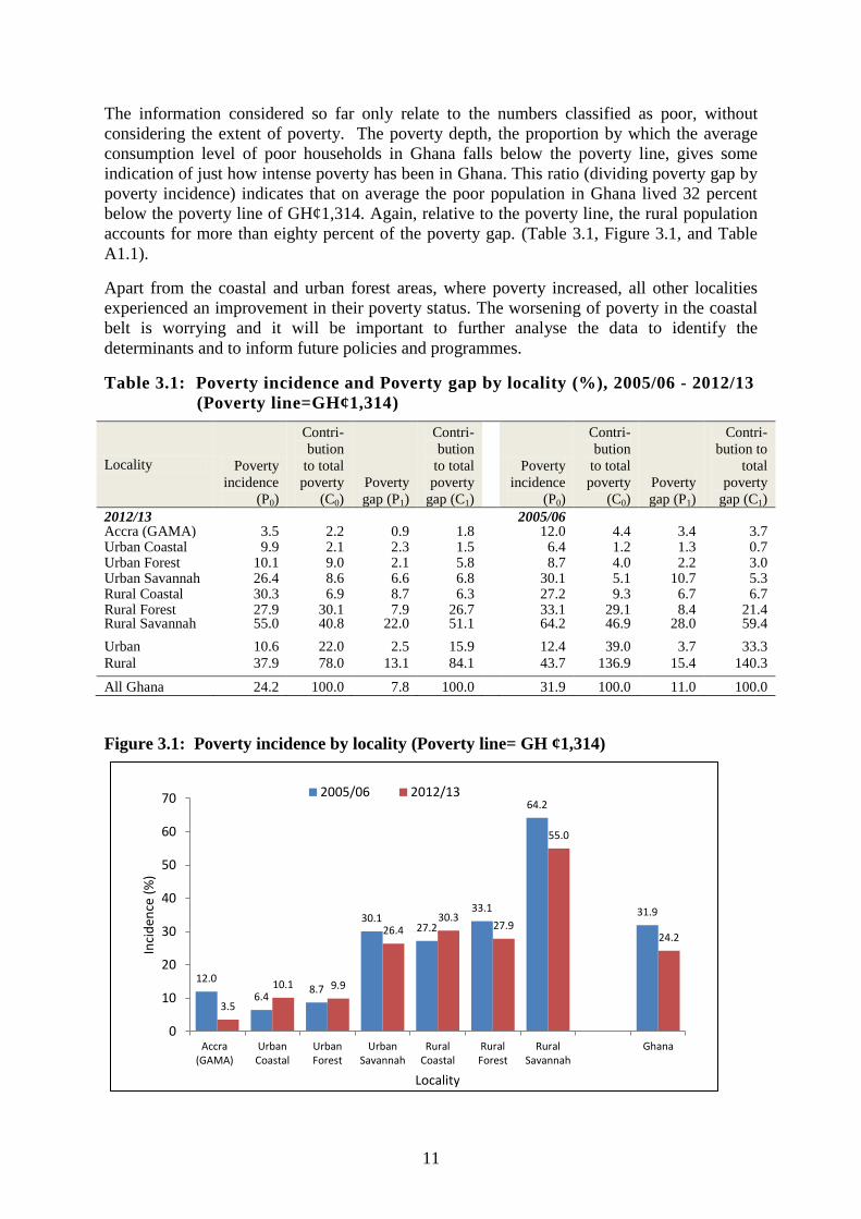
Apart from the coastal and urban forest areas, where poverty increased, all other localities
experienced an improvement in their poverty status. The worsening of poverty in the coastal
belt is worrying and it will be important to further analyse the data to identify the
determinants and to inform future policies and programmes.
Table 3.1: Poverty incidence and Poverty gap by locality (%), 2005/06 - 2012/13
(Poverty line=GH¢1,314)
Locality Poverty
incidence
(P0)
Contri-
bution
to total
poverty
(C0)
Poverty
gap (P1)
Contri-
bution
to total
poverty
gap (C1)
Poverty
incidence
(P0)
Contri-
bution
to total
poverty
(C0)
Poverty
gap (P1)
Contri-
bution to
total
poverty
gap (C1)
2012/13
2005/06 Accra (GAMA) 3.5 2.2 0.9 1.8
12.0 4.4 3.4 3.7
Urban Coastal 9.9 2.1 2.3 1.5
6.4 1.2 1.3 0.7 Urban Forest 10.1 9.0 2.1 5.8
8.7 4.0 2.2 3.0
Urban Savannah 26.4 8.6 6.6 6.8
30.1 5.1 10.7 5.3 Rural Coastal 30.3 6.9 8.7 6.3
27.2 9.3 6.7 6.7
Rural Forest 27.9 30.1 7.9 26.7
33.1 29.1 8.4 21.4 Rural Savannah 55.0 40.8 22.0 51.1
64.2 46.9 28.0 59.4
Urban 10.6 22.0 2.5 15.9
12.4 39.0 3.7 33.3
Rural 37.9 78.0 13.1 84.1
43.7 136.9 15.4 140.3
All Ghana 24.2 100.0 7.8 100.0 31.9 100.0 11.0 100.0
Figure 3.1: Poverty incidence by locality (Poverty line= GH ¢1,314)
12.0
6.4 8.7
30.1 27.2
33.1
64.2
31.9
3.5
10.1 9.9
26.4 30.3
27.9
55.0
24.2
0
10
20
30
40
50
60
70
Accra(GAMA)
UrbanCoastal
UrbanForest
UrbanSavannah
RuralCoastal
RuralForest
RuralSavannah
Ghana
Inci
den
ce (
%)
Locality
2005/06 2012/13

12
3.3 Extreme Poverty in Ghana
Extreme poverty is defined as those whose standard of living is insufficient to meet their
basic nutritional requirements even if they devoted their entire consumption budget to food.
Table 3.2 illustrates the incidence of extreme poverty for the country as a whole and for the
seven geographic localities. Given the extreme poverty line of GH¢792.05 per adult
equivalent per year, an estimated 8.4 percent of Ghanaians are considered to be extremely
poor. This rate indicates that fewer Ghanaians are extremely poor compared to 2005/06.
Revising the extreme poverty line based on the current basket of food consumed by
Ghanaians, the incidence of extreme poverty reduced by 8.1 percentage points from the
2005/06 revised extreme poverty incidence of 16.5 percent.
More than 2.2 million Ghanaians (based on 2010 PHC projections) cannot afford to feed
themselves with 2,900 calories per adult equivalent of food per day, even if they were to
spend all their expenditures on food. Although the absolute number living in extreme poverty
has reduced over time, it is still quite high given the fact that Ghana is considered to be a
lower middle income country.
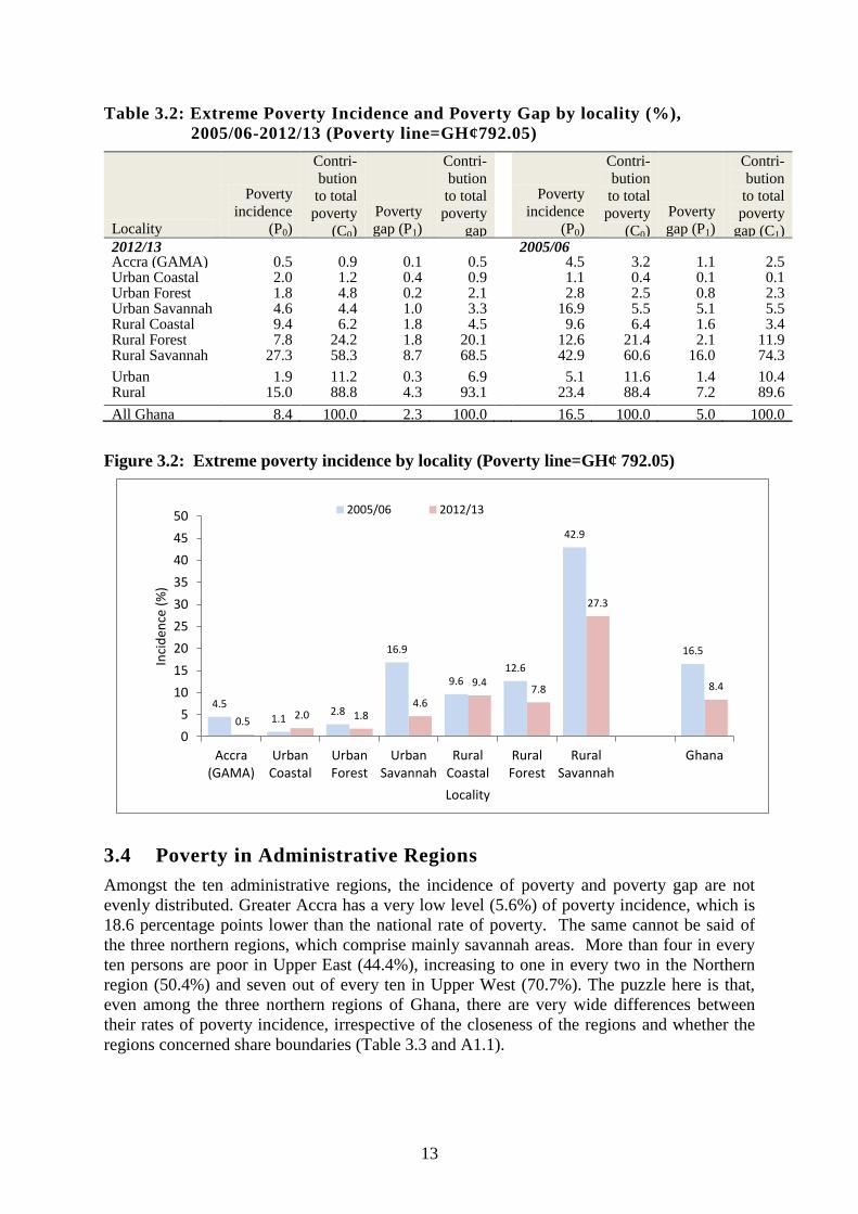
The sharp geographic variations that characterize absolute poverty are found to be more
pronounced with extreme poverty, with the incidence of extreme poverty being highest in
rural Savannah. Extreme poverty is also a rural phenomenon, with as many as over 1.8
million persons living in extreme poverty in rural areas (2010 PHC projections). Extreme
poverty is particularly high in rural Savannah at 27.3 percent and this locality accounts for
nearly three-fifths of those living in extreme poverty in Ghana. The incidence of extreme
poverty is virtually non-existence in urban localities, with Accra (GAMA) contributing only
0.9 percent to the incidence of extreme poverty. Urban localities contribute 11.2 percent to
the national incidence of extreme poverty (Table 3.2 and A1.2).
13
Table 3.2: Extreme Poverty Incidence and Poverty Gap by locality (%),
2005/06-2012/13 (Poverty line=GH¢792.05)
Locality
Poverty
incidence
(P0)
Contri-
bution
to total
poverty
(C0)
Poverty
gap (P1)
Contri-
bution
to total
poverty
gap
(C1)
Poverty
incidence
(P0)
Contri-
bution
to total
poverty
(C0)
Poverty
gap (P1)
Contri-
bution
to total
poverty
gap (C1) 2012/13
2005/06
Accra (GAMA) 0.5 0.9 0.1 0.5
4.5 3.2 1.1 2.5 Urban Coastal 2.0 1.2 0.4 0.9
1.1 0.4 0.1 0.1
Urban Forest 1.8 4.8 0.2 2.1
2.8 2.5 0.8 2.3 Urban Savannah 4.6 4.4 1.0 3.3
16.9 5.5 5.1 5.5
Rural Coastal 9.4 6.2 1.8 4.5
9.6 6.4 1.6 3.4 Rural Forest 7.8 24.2 1.8 20.1
12.6 21.4 2.1 11.9
Rural Savannah 27.3 58.3 8.7 68.5
42.9 60.6 16.0 74.3
Urban 1.9 11.2 0.3 6.9
5.1 11.6 1.4 10.4 Rural 15.0 88.8 4.3 93.1
23.4 88.4 7.2 89.6
All Ghana 8.4 100.0 2.3 100.0 16.5 100.0 5.0 100.0
Figure 3.2: Extreme poverty incidence by locality (Poverty line=GH¢ 792.05)
3.4 Poverty in Administrative Regions
Amongst the ten administrative regions, the incidence of poverty and poverty gap are not
evenly distributed. Greater Accra has a very low level (5.6%) of poverty incidence, which is
18.6 percentage points lower than the national rate of poverty. The same cannot be said of
the three northern regions, which comprise mainly savannah areas. More than four in every
ten persons are poor in Upper East (44.4%), increasing to one in every two in the Northern
region (50.4%) and seven out of every ten in Upper West (70.7%). The puzzle here is that,
even among the three northern regions of Ghana, there are very wide differences between
their rates of poverty incidence, irrespective of the closeness of the regions and whether the
regions concerned share boundaries (Table 3.3 and A1.1).
4.5
1.1 2.8
16.9
9.6 12.6
42.9
16.5
0.5 2.0 1.8
4.6
9.4 7.8
27.3
8.4
0
5
10
15
20
25
30
35
40
45
50
Accra(GAMA)
UrbanCoastal
UrbanForest
UrbanSavannah
RuralCoastal
RuralForest
RuralSavannah
Ghana
Inci
den
ce (
%)
Locality
2005/06 2012/13

14
However, even though poverty in the Upper West region is highest amongst the ten regions,
the region contributes less than ten percent to the national poverty due to the fact that it is the
smallest region in Ghana in terms of population. Indeed, of the 6.4 million persons who are
deemed poor in Ghana, only half a million are from the Upper West region, whilst the
Northern region with a poverty incidence of 50.4 percent accounts for one-fifth (20.8%) or
1.3 million of the poor in Ghana, making this region the highest single contributor to the level
of poverty in Ghana. This pattern does not seem any different from 2005/06, since the
northern region again was the highest contributor to national poverty (Table 3.3 and A1.1).
In terms of extreme poverty incidence, apart from the three northern regions, whose rates are
higher than the national rate of extreme poverty, all the other regions in the coastal and forest
areas have rates lower than the national average. Upper West region has the highest extreme
poverty incidence of 45.1 percent, followed by Northern (22.8%) and Upper East (21.3%)
(Table 3.4 and A1.2).
In terms of contribution to extreme poverty, the Northern region accounts for slightly over a
quarter of the extreme poor in Ghana, far more than any other region. The three northern
regions combined account for more than half of those living in extreme poverty (52.7%). The
pattern is very similar to the findings in 2005/06, although the three northern regions account
for slightly less of the extreme poor in 2012/13 than in 2005/06 (Table 3.4 and A1.2).
Table 3.3: Poverty incidence and poverty gap by region (%), 2005/06 -2012/13
(Poverty line=GH¢1,314)
Region
Poverty
incidence
(P0)
Contri-
bution
to total
poverty
(C0)
Poverty
gap (P1)
Contri-
bution to
total
poverty
gap (C1)
Poverty
incidence
(P0)
Contri-
bution
to total
poverty
(C0)
Poverty
gap (P1)
Contri-
bution
to total
poverty
gap
(C1) 2012/13
2005/06 Western 20.9 7.9 5.7 6.8
22.9 7.3 5.4 5.0
Central 18.8 6.9 5.6 6.4
23.4 6.4 5.6 4.4 Greater Accra 5.6 3.8 1.6 3.5
13.5 5.9 3.7 4.7
Volta 33.8 12.1 9.8 11.0
37.3 8.7 9.2 6.2 Eastern 21.7 9.3 5.8 7.8
17.8 7.5 4.2 5.2
Ashanti 14.8 12.0 3.5 9.0
24.0 12.6 6.4 9.8 Brong Ahafo 27.9 11.4 7.4 9.4
34.0 9.8 9.5 7.9
Northern 50.4 20.8 19.3 24.9
55.7 21.0 23.0 25.2 Upper East 44.4 7.4 17.2 9.0
72.9 10.9 35.3 15.3
Upper West 70.7 8.4 33.2 12.3
89.1 10.0 50.7 16.4
All Ghana 24.2 100.0 7.8 100.0 31.9 100.0 11.0 100.0

15
Figure 3.3: Poverty incidence by region (Poverty line=GH¢1,314)
Table 3.4: Extreme Poverty incidence and poverty gap by region (%),
2005/06 - 2012/13 (Poverty line= GH¢792.05)
Region
Poverty
incidence
(P0)
Contri-
bution to
total
poverty
(C0)
Poverty
gap
(P1)
Contri-
bution to
total
poverty
gap (C1)
Poverty
incidence
(P0)
Contri-
bution to
total
poverty
(C0)
Poverty
gap
(P1)
Contri-
bution
to total
poverty
gap
(C1) 2012/13
2005/06
Western 5.5 6.0 1.3 5.1
6.8 4.2 1.3 2.7 Central 6.8 7.1 1.5 5.9
7.6 4.0 1.1 1.9
Greater Accra 1.5 2.9 0.3 2.1
5.2 4.4 1.1 2.9 Volta 9.0 9.3 1.9 7.2
13.3 6.0 2.2 3.3
Eastern 6.0 7.3 1.3 5.8
5.8 4.7 1.2 3.3 Ashanti 2.9 6.9 0.5 4.5
9.8 9.9 1.8 6.2
Brong Ahafo 6.6 7.8 1.5 6.5
13.7 7.6 2.9 5.3 Northern 22.8 27.0 7.2 31.5
36.1 26.3 12.1 29.1
Upper East 21.3 10.3 6.9 12.3
56.9 16.4 21.3 20.2 Upper West 45.1 15.4 15.3 19.3
76.0 16.4 35.4 25.1
All Ghana 8.4 100.0 2.3 100.0 16.5 100.0 5.0 100.0
22.9 23.4
13.5
37.3
17.8
24.0
34.0
55.7
72.9
89.1
31.9
20.9 18.8
5.6
33.8
21.7
14.8
27.9
50.4
44.4
70.7
24.2
0
10
20
30
40
50
60
70
80
90
100
Western Central GreaterAccra
Volta Eastern Ashanti BrongAhafo
Northern Upper East UpperWest
Ghana
Inci
den
ce (
%)
Region
2005/06 2012/13

16
Figure 3.4: Extreme poverty incidence by locality (Poverty line=GH¢792.05)
Figure 3.5: Extreme poverty incidence by region (Poverty line=GH¢792.05)
4.5
1.1 2.8
16.9
9.6
12.6
42.9
16.5
0.5 1.9 1.8
4.6
9.3 7.8
27.3
8.4
0
5
10
15
20
25
30
35
40
45
50
Accra(GAMA)
UrbanCoastal
UrbanForest
UrbanSavannah
RuralCoastal
RuralForest
RuralSavannah
Ghana
Inci
den
ce (
in %
)
Locality
2005/06 2012/13
6.8 7.6 5.2
13.3
5.8 9.8
13.7
36.1
56.9
76.0
16.5
5.5 6.8
1.5
9.0 6.0
2.9 6.6
22.8 21.3
45.1
8.4
0
10
20
30
40
50
60
70
80
Western Central GreaterAccra
Volta Eastern Ashanti BrongAhafo
Northern UpperEast
UpperWest
Ghana
Inci
den
ce (
in %
)
Region
2005/06 2012/13

17
3.5 Summary
About a quarter of Ghanaians are poor whilst under a tenth of the population are in extreme
poverty. Although the level of extreme poverty is relatively low, it is concentrated in Rural
Savannah, with more than a quarter of the people being extremely poor. Overall, the
dynamics of poverty in Ghana over the 7-year period indicate that poverty is still very much a
rural phenomenon, thus reducing rural poverty is a panacea to Ghana’s poverty, if poverty
reduction is to achieve the desired levels for Ghana as a middle income country.
There is a lot of variability in poverty incidence by region. Whilst half of the ten regions
(Greater Accra, Western, Central, Eastern, and Ashanti) had their rates of poverty incidence
lower than the national average of 24.2 percent, the remaining half had rates higher than the
national average; Greater Accra is the least poor region and the Upper West the poorest
overall. Though most regions show a reduction in poverty incidence since 2005/06, the
pattern of poverty by region has not changed.

18
CHAPTER FOUR
COVARIATE ANALYSIS
4.1 Decomposition of Poverty
For a given poverty line, changes in a poverty index can be expressed in terms of: (a) the
observed change in the mean value of the standard of living measure, assuming that
inequality had remained unchanged (“growth” effect); (b) the observed change in inequality,
assuming that the mean value had remained unchanged (redistribution effect).
It is good to have a nation experience increases in output and therefore higher economic
growth, but whether a lot of people participated in the growth process is indeed as critical as
the growth itself. Growth in the average standard of living will reduce poverty, all things
being equal, but where it is accompanied by an increase in inequality, the reduction in
poverty will not be as pronounced. The effectiveness of growth in poverty reduction is
increased where that growth is pro-poor, in other words, when it is accompanied by falling
inequality. To what extent do changes in poverty in Ghana reflect changes in the average
living standard, and what role have changes in inequality played? The answer to these
questions can be obtained when the changes in the poverty rates are decomposed into growth
and inequality effect.
To establish the source of poverty reduction, this report decomposed the poverty reduction at
the national level as well as in urban/rural areas. At the national level, the 7.7 percentage
point reduction in poverty incidence was found to be due to the growth effect. Indeed, but for
the worsening inequality, poverty would have decreased by 8.8 percentage points, since
inequality contributed to worsening poverty by 1.1 percentage points. The same argument
holds for both rural and urban localities. The case is even worse for the rural localities where
poverty was highest. Poverty among the rural localities would have reduced by 8.8
percentage points instead of the current 5.8 percentage points in the 7-year period if
inequality did not worsen over the period.
Table 4.1: Decomposition of change in poverty headcount by urban/rura l
residence (%), 2005 - 2013
Place of
residence Total change
Share of change due to:
Growth Redistribution
National -7.7 -8.8 1.1
Urban -1.9 -2.4 0.5
Rural -5.8 -8.8 3.0
4.2 Poverty by economic activity and gender of household head
In addition to the geographic pattern of poverty incidence and gap discussed earlier, it is also
important to relate poverty rates to the economic activities in which households are engaged.
Figure 4.1 presents the incidence of poverty by the main economic activity of the household
head. The poverty incidence is highest among households where the head is engaged as self-
employed in the agricultural sector. Households whose heads are paid employees, self-
employed in the non-agricultural sector or retired are less likely to be poor. Even though
farmers experienced some reduction in poverty over the 7-year period, they are still the
19
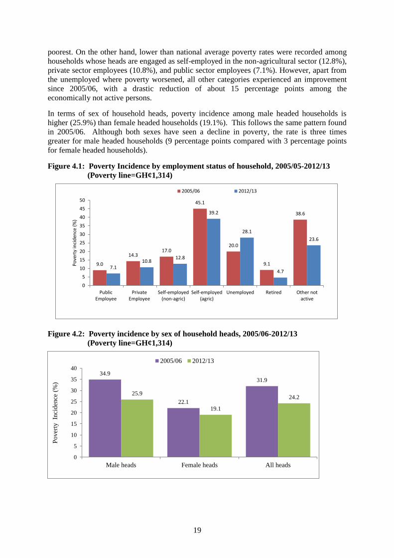
poorest. On the other hand, lower than national average poverty rates were recorded among
households whose heads are engaged as self-employed in the non-agricultural sector (12.8%),
private sector employees (10.8%), and public sector employees (7.1%). However, apart from
the unemployed where poverty worsened, all other categories experienced an improvement
since 2005/06, with a drastic reduction of about 15 percentage points among the
economically not active persons.
In terms of sex of household heads, poverty incidence among male headed households is
higher (25.9%) than female headed households (19.1%). This follows the same pattern found
in 2005/06. Although both sexes have seen a decline in poverty, the rate is three times
greater for male headed households (9 percentage points compared with 3 percentage points
for female headed households).
Figure 4.1: Poverty Incidence by employment status of household, 2005/05-2012/13
(Poverty line=GH¢1,314)
Figure 4.2: Poverty incidence by sex of household heads, 2005/06-2012/13
(Poverty line=GH¢1,314)
9.0
14.3 17.0
45.1
20.0
9.1
38.6
7.1 10.8
12.8
39.2
28.1
4.7
23.6
0
5
10
15
20
25
30
35
40
45
50
PublicEmployee
PrivateEmployee
Self-employed(non-agric)
Self-employed(agric)
Unemployed Retired Other notactive
Po
vert
y in
cid
ence
(%
)
2005/06 2012/13
34.9
22.1
31.9
25.9
19.1
24.2
0
5
10
15
20
25
30
35
40
Male heads Female heads All heads
Po
ver
ty
Inci
den
ce (
%)
2005/06 2012/13
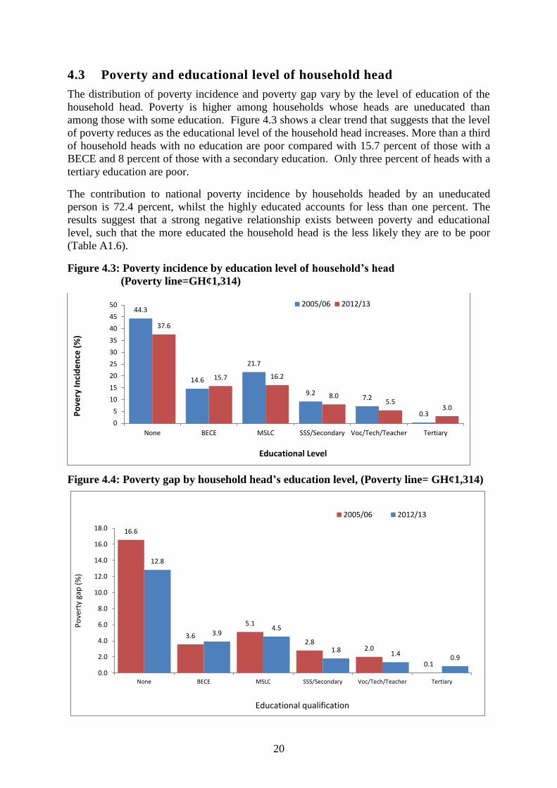
20
4.3 Poverty and educational level of household head
The distribution of poverty incidence and poverty gap vary by the level of education of the
household head. Poverty is higher among households whose heads are uneducated than
among those with some education. Figure 4.3 shows a clear trend that suggests that the level
of poverty reduces as the educational level of the household head increases. More than a third
of household heads with no education are poor compared with 15.7 percent of those with a
BECE and 8 percent of those with a secondary education. Only three percent of heads with a
tertiary education are poor.
The contribution to national poverty incidence by households headed by an uneducated
person is 72.4 percent, whilst the highly educated accounts for less than one percent. The
results suggest that a strong negative relationship exists between poverty and educational
level, such that the more educated the household head is the less likely they are to be poor
(Table A1.6).
Figure 4.3: Poverty incidence by education level of household’s head
(Poverty line=GH¢1,314)
Figure 4.4: Poverty gap by household head’s education level, (Poverty line= GH¢1,314)
44.3
14.6
21.7
9.2 7.2
0.3
37.6
15.7 16.2
8.0 5.5
3.0
0
5
10
15
20
25
30
35
40
45
50
None BECE MSLC SSS/Secondary Voc/Tech/Teacher Tertiary
Po
very
Inci
de
nce
(%
)
Educational Level
2005/06 2012/13
16.6
3.6
5.1
2.8 2.0
0.1
12.8
3.9 4.5
1.8 1.4 0.9
0.0
2.0
4.0
6.0
8.0
10.0
12.0
14.0
16.0
18.0
None BECE MSLC SSS/Secondary Voc/Tech/Teacher Tertiary
Po
vert
y ga
p (
%)
Educational qualification
2005/06 2012/13
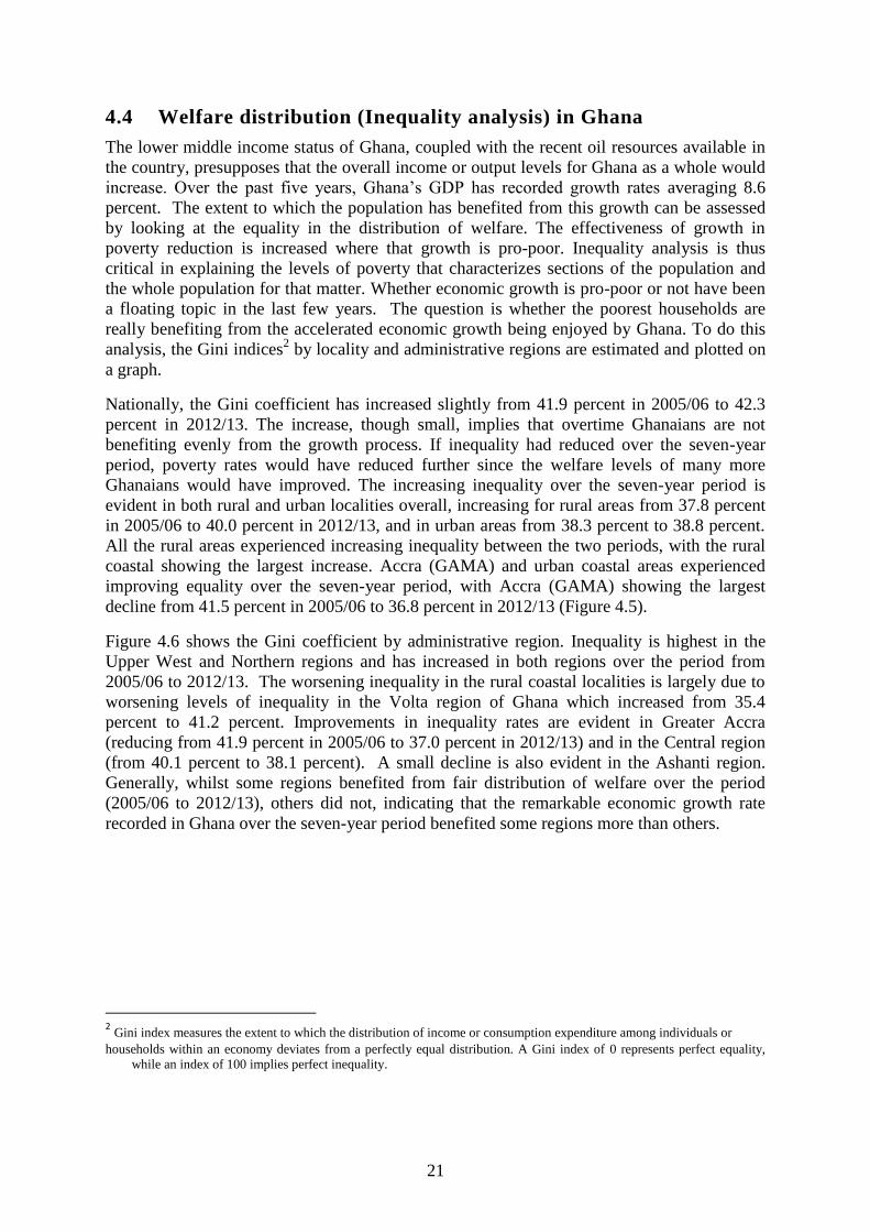
21
4.4 Welfare distribution (Inequality analysis) in Ghana
The lower middle income status of Ghana, coupled with the recent oil resources available in
the country, presupposes that the overall income or output levels for Ghana as a whole would
increase. Over the past five years, Ghana’s GDP has recorded growth rates averaging 8.6
percent. The extent to which the population has benefited from this growth can be assessed
by looking at the equality in the distribution of welfare. The effectiveness of growth in
poverty reduction is increased where that growth is pro-poor. Inequality analysis is thus
critical in explaining the levels of poverty that characterizes sections of the population and
the whole population for that matter. Whether economic growth is pro-poor or not have been
a floating topic in the last few years. The question is whether the poorest households are
really benefiting from the accelerated economic growth being enjoyed by Ghana. To do this
analysis, the Gini indices2 by locality and administrative regions are estimated and plotted on
a graph.
Nationally, the Gini coefficient has increased slightly from 41.9 percent in 2005/06 to 42.3
percent in 2012/13. The increase, though small, implies that overtime Ghanaians are not
benefiting evenly from the growth process. If inequality had reduced over the seven-year
period, poverty rates would have reduced further since the welfare levels of many more
Ghanaians would have improved. The increasing inequality over the seven-year period is
evident in both rural and urban localities overall, increasing for rural areas from 37.8 percent
in 2005/06 to 40.0 percent in 2012/13, and in urban areas from 38.3 percent to 38.8 percent.
All the rural areas experienced increasing inequality between the two periods, with the rural
coastal showing the largest increase. Accra (GAMA) and urban coastal areas experienced
improving equality over the seven-year period, with Accra (GAMA) showing the largest
decline from 41.5 percent in 2005/06 to 36.8 percent in 2012/13 (Figure 4.5).
Figure 4.6 shows the Gini coefficient by administrative region. Inequality is highest in the
Upper West and Northern regions and has increased in both regions over the period from
2005/06 to 2012/13. The worsening inequality in the rural coastal localities is largely due to
worsening levels of inequality in the Volta region of Ghana which increased from 35.4
percent to 41.2 percent. Improvements in inequality rates are evident in Greater Accra
(reducing from 41.9 percent in 2005/06 to 37.0 percent in 2012/13) and in the Central region
(from 40.1 percent to 38.1 percent). A small decline is also evident in the Ashanti region.
Generally, whilst some regions benefited from fair distribution of welfare over the period
(2005/06 to 2012/13), others did not, indicating that the remarkable economic growth rate
recorded in Ghana over the seven-year period benefited some regions more than others.
2 Gini index measures the extent to which the distribution of income or consumption expenditure among individuals or
households within an economy deviates from a perfectly equal distribution. A Gini index of 0 represents perfect equality,
while an index of 100 implies perfect inequality.
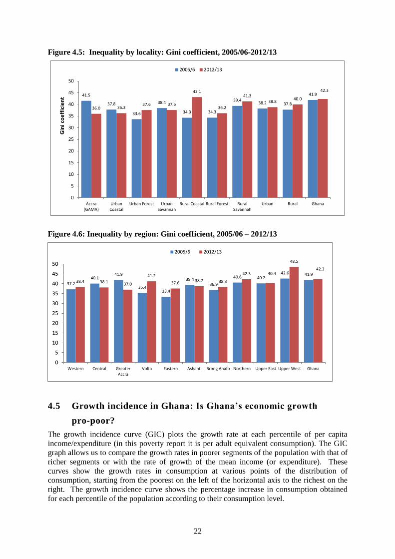
22
Figure 4.5: Inequality by locality: Gini coefficient, 2005/06-2012/13
Figure 4.6: Inequality by region: Gini coefficient, 2005/06 – 2012/13
4.5 Growth incidence in Ghana: Is Ghana’s economic growth
pro-poor?
The growth incidence curve (GIC) plots the growth rate at each percentile of per capita
income/expenditure (in this poverty report it is per adult equivalent consumption). The GIC
graph allows us to compare the growth rates in poorer segments of the population with that of
richer segments or with the rate of growth of the mean income (or expenditure). These
curves show the growth rates in consumption at various points of the distribution of
consumption, starting from the poorest on the left of the horizontal axis to the richest on the
right. The growth incidence curve shows the percentage increase in consumption obtained
for each percentile of the population according to their consumption level.
41.5
37.8
33.6
38.4
34.3 34.3
39.4 38.2 37.8
41.9
36.0 36.3 37.6 37.6
43.1
36.2
41.3 38.8
40.0
42.3
0
5
10
15
20
25
30
35
40
45
50
Accra(GAMA)
UrbanCoastal
Urban Forest UrbanSavannah
Rural Coastal Rural Forest RuralSavannah
Urban Rural Ghana
Gin
i co
eff
icie
nt
2005/6 2012/13
37.2 40.1
41.9
35.4 33.4
39.4 36.9
40.6 40.2 42.6 41.9
38.4 38.1 37.0
41.2
37.6 38.7 38.3
42.3 40.4
48.5
42.3
0
5
10
15
20
25
30
35
40
45
50
Western Central GreaterAccra
Volta Eastern Ashanti Brong Ahafo Northern Upper East Upper West Ghana
2005/6 2012/13

23
Figure 4.7 shows that growth rates in consumption (per adult equivalent) have been
significantly higher in the two extreme ends of the distribution (the upper part of the
population, and the very poor), indicating that both the upper echelons and below the 10th
quintile of the population benefited from very large gains in consumption. Generally,
however, the majority of the population between the 10th
and the 80th
percentile had a growth
in consumption of about 8.5 percent, indicating that growth was evenly distributed as the
pattern of gains was equitable for a fairly large segment of the population. Growth in
consumption has been good for even those within the very extreme end of the population (95
-100 quintile), since growth in consumption was higher than 7.2 percent. Every segment of
the quintile population had positive growth in consumption of more than 7 percent. Figure 4.7
suggests a growing middle class in Ghana.
The GIC takes a similar shape for urban and rural areas when they are assessed separately. In
both areas, the population at the 60th percentile and above enjoyed a much higher growth rate
than the rest of the population. It should be noted that these households are not poor
households and the high growth rates among them indicate an emergence of the middle class
in Ghana.
Has economic growth in Ghana over the seven-year period (2005/06 – 2012/13) been pro-
poor? The economic literature does not fully agree on what should be labeled pro-poor
growth. On one side, researchers want economic growth to be faster for the poor than the
richer households for growth to be defined as pro-poor growth (leading to a decline in
inequality); others look at whether growth has raised the welfare level of all households as
measured per percentile. Based on the latter definition, Ghana has clearly experienced pro-
poor growth since all percentiles benefited from economic growth even though the rates
varied.
Figures 4.8 and 4.9 show the growth incidence curves for the urban and rural localities. The
results indicate that the distribution has been similar for both urban and rural localities.
Except in the urban localities, the poor benefited more as they experienced a higher growth in
consumption, whilst households in the rural areas recorded higher growth in the upper
echelons of the population.
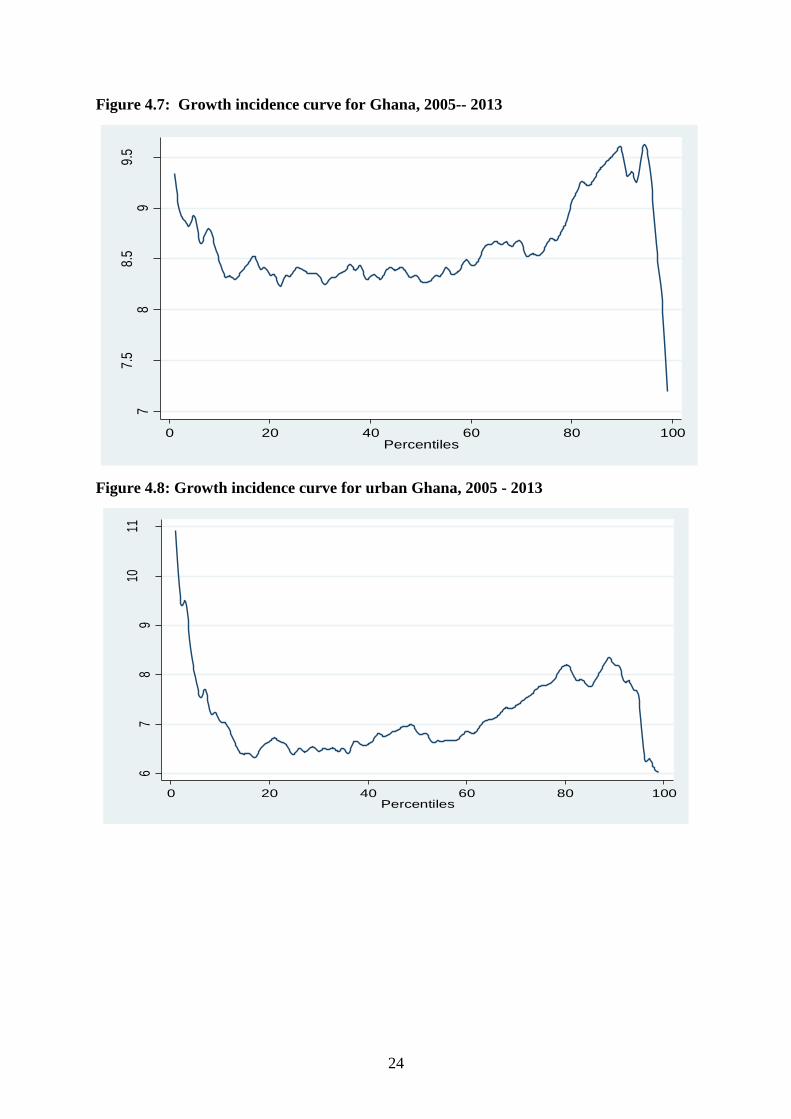
24
Figure 4.7: Growth incidence curve for Ghana, 2005-- 2013
Figure 4.8: Growth incidence curve for urban Ghana, 2005 - 2013
77.
58
8.5
99.
5
Med
ian
splin
e
0 20 40 60 80 100Percentiles
67
89
1011
Med
ian
splin
e
0 20 40 60 80 100Percentiles

25
Figure 4.9: Growth incidence curve for rural Ghana, 2005 - 2013
4.6 Summary
Household heads who are farmers are not just the poorest in Ghana, but they contribute the
most to Ghana’s poverty. Household heads engaged as private employees and self-employed
in non-agricultural sectors are less likely to be poor than those engaged in the agricultural
sector. Over the period, public sector earners have, as a result of the public sector wage
rationalization policy implemented in 2009, experienced a reduction in poverty.
Generally, female-headed households appear to be better off than male-headed households in
terms of poverty incidence. Lack of education is still a hindrance to poverty reduction.
Households with uneducated household heads are the poorest in Ghana and contribute the
most to Ghana’s poverty incidence.
Welfare distribution is more disproportionate in Ghana now than in 2005/06; this means that
there is increasing inequality as measured by the Gini coefficient. However, whilst some
regions showed improvement in terms of the equality in the distribution of welfare, other
regions such as Volta and Upper West experienced worsening welfare distribution between
2005/06 and 2012/13. Generally, those in the lower income brackets and the population
above the 60th
percentile benefited the most from the growth in consumption. The growth
incidence curve shows a growing middle class in the Ghanaian population.
78
91
0
Me
dia
n s
plin
e
0 20 40 60 80 100Percentiles

26
CHAPTER FIVE
HOUSEHOLD ASSETS
5.1 Introduction
Chapter three of this report has shown that the incidence of poverty – measured in terms of
consumption expenditure – has declined in Ghana between 2005/06 and 2012/13, although
this reduction has not been uniformly spread across the country.
Poverty is a multi-dimensional phenomenon and consumption-based measures need to be
supplemented by other welfare indicators. This section examines poverty in terms of
household ownership of key consumer durable goods which can be seen as an alternative
measure of poverty to the consumption-based measures of welfare presented in previous
chapters. One of the advantages of these asset-based indicators is the ease with which they
can be measured compared to the indicators based on consumption expenditure.
This chapter considers a measure that captures changes in household ownership of such
assets as an indicator of changing living standards of households3. Although this measure
depends on many factors outside the control of households such as whether or not they have
access to electricity and other location and cultural attributes that shape lifestyles but cannot
be changed easily by households, it is still a useful proxy indicator of the standard of living.
5.2 Asset Ownership
Information on the proportion of households owning different consumer durable goods in
1998/99, 2005/06 and 2012/2013 is presented in Figures 5.1 and 5.2 for urban and rural areas
respectively (see Tables A2.1, to A2.4). The data presented in these graphs refer to ownership
of at least one of such items and does not directly depict the total number of items that are in
the possession of households during the survey periods. For most of the assets considered,
there is an increase in the proportion of households owning the asset over the fifteen-year
period. This is particularly the case for items like stove, fridge, television, computer and
mobile phones.
Spatial analysis of the information in Figures 5.1 and 5.2 show that the proportion of
households owning these assets continues to be much higher in urban areas than in rural
areas. The pattern of changes between ownership of assets in the last two surveys i.e. 2005/06
and 2012/13 is also different for urban and rural households. Whereas the increases in
ownership of items are relatively higher for most of the assets in both localities, the increase
in stove ownership is more pronounced in urban areas than in rural areas. In urban areas,
nearly nine in every ten households now own a mobile phone, an increase from just over one
third in 2005/06; the increase in mobile phone ownership is more pronounced in rural areas
with an increase from 6 percent in 2005/06 to 70 percent in 2012/13. After peaking in
2005/06, ownership of radio sets decreased marginally in 2012/2013 for both urban and rural
areas whereas ownership of sewing machines in both localities has decreased over the last
fifteen years.
3 Note that the tables presented are based on changes in the proportion of households in a given group
owning an asset, rather than acquisition of assets by individual households (which is harder to measure
from the questionnaire).

27
Figure 5.1: Percentage of urban households owning different household assets,
1998/99-2012/13
Source: Table A2.3
Figure 5.2: Percentage of rural households owning different household assets,
1998/99-2012/13
Source: Table A2.4
The distribution of ownership of transportation assets by locality shows marginal increases in
urban and rural areas over the past fifteen years. Despite this, in urban areas 7 percent of
households owned a car in 2012/13 compared to only 2 percent of those in rural areas. The
increase is higher for ownership of bicycles in rural areas than urban areas (Figure 5.3 and
5.4).
33
23
33
45
63
40
5 0 0
24
33
39
54
77
53
5
36
4
17
46
53
69 65
75
4
88
18
0
10
20
30
40
50
60
70
80
90
100
Sewingmachine
Stove Fridge Fan Radio TV Camera Mobilephone
Computer
1998/99 2005/06 2012/13
29
7 7 11
47
12
1 0 0
18
7 8 12
71
14
2 6
1
14 10
15
25
67
34
1
70
4
0
10
20
30
40
50
60
70
80
Sewingmachine
Stove Fridge Fan Radio TV Camera Mobilephone
Computer
1998/99 2005/06 2012/13

28
Figure 5.3: Percentage of urban households owning different transportation assets,
1998/99-2012/13
Source: Table A2.3
Figure 5.4: Percentage of rural households owning different transportation assets,
1998/99-2012/13
Source: Table A2.4
More information can be provided by examining specific durable goods in greater detail.
Figures 5.5 and 5.6 examine ownership of two such groups, one being a useful productive
asset for the household (refrigerator) while the other is more for pleasure and information
(television set). Figures for all other durable goods under study can be found in the appendix.
12
1
5
14
2
5
14
6
7
0
2
4
6
8
10
12
14
16
Bicycle Motocycle Car
Per
cen
t (%
)
1998/99 2005/06 2012/13
23
1 1
29
2 1
28
9
2
0
5
10
15
20
25
30
35
Bicycle Motocycle Car
Per
cen
t (%
)
1998/99 2005/06 2012/13

29
Figure 5.5: Percentage of households owning a refrigerator by locality and
quintile, 1998/99-2012/13
Figure 5.6: Percentage of households owning a television set by locality and
quintile, 1998/99-2012/13
2 5
20
31
44
0 1 6
10
17
10
17
25
34
51
1 4 6
10
19 18
29
42
52
68
3
9
15
22
33
0
10
20
30
40
50
60
70
80
UrbanLowest
UrbanSecond
UrbanThird
UrbanFourth
UrbanHighest
RuralLowest
RuralSecond
RuralThird
RuralFourth
RuralHighest
Per
cen
t (%
)
1998/99 2005/06 2012/13
6
16
35
41
48
1 6
12 15
25 23
33
42
52
63
2
10 13
19
30
39
55
69
79
86
17
27
36
45
54
0
10
20
30
40
50
60
70
80
90
100
UrbanLowest
UrbanSecond
UrbanThird
UrbanFourth
UrbanHighest
RuralLowest
RuralSecond
RuralThird
RuralFourth
RuralHighest
Per
cen
t (%
)
1998/99 2005/06 2012/13

30
The figures present the changes in ownership of these assets for different quintile4 groups of
households defined according to their standards of living.
The distribution of assets among quintiles across the survey periods shows increases in the
proportion of households who own durable goods. These increases are more dramatic in the
last 5 years, especially for refrigerator and TV set (Figure 5.5 and 5.6) across all locality and
quintile groups. The information in Appendix 2 and Tables A2.2 to A2.4 further show a
reduction in the proportion of households who own sewing machines, radios and bicycles
over the survey period.
5.3 Summary
The proportions of households owning most of the durable goods covered in the surveys have
shown large increases between 1998/99 and 2005/2006, and further increases in 2012/13. The
increases were observed in both urban and rural areas but they have often been higher for
wealthier groups, with greater disparity among urban households. Ownership of durable
goods remains much lower in rural areas than urban areas, even among households of similar
overall living standards.
4 For each of these non-monetary measures, it is valuable to look at the relationship between the variations in
living conditions they reveal and those of the consumption-based standard of living measure. This is considered
here based on the division of households into quintile groups reflecting their standard of living according to the
consumption-based measure. The lowest quintile group represents the poorest 20% of individuals in the
population, the second quintile the next poorest 20% and so on until the highest quintile which contains the
richest 20%. These groups are defined at the national level throughout; whenever results are presented by
quintile group for urban and rural areas separately, the quintile groups are still those defined at the national
level. Therefore, for example, those in urban areas reported as being in the fifth quintile have comparable living
standards to those in the fifth quintile in rural areas.

31
CHAPTER SIX
ACCESS TO SERVICES
6.1 Introduction
In previous chapters, the GLSS 6 data are used to demonstrate improvements in Ghanaian
living standards based on the household’s total consumption and ownership of household
assets. Access to services, which is part of the MDG indicators, is another important element
used to evaluate or determine whether living standards have improved, especially among
households living at the bottom consumption quintiles. This chapter analyzes households’
access to potable water (defined to include pipe, bottle/sachet, protected well/spring, and
borehole), adequate toilet facility (a flush toilet or the KVIP toilet) and electricity.
6.2 Household access to utilities and sanitation facilities
Access to services is determined both by their availability and affordability. Availability of
services is largely determined by their locations because infrastructure is available within
proximity. Urban areas normally have much more service availability than rural areas. For
this reason, one should compare access to services interactively by locality and quintiles.
Affordability is largely determined by the households’ ability to pay for available services,
and ability to pay is itself determined by cost and by income. Figures 6.1, 6.2 and 6.3
provide information on the proportion of households using potable water and adequate toilet
facilities and having access to electricity.
Figure 6.1 shows the percentage of households using potable water by locality and standard
of living quintiles. It indicates that, overall, about 95 percent of urban households and 75
percent of rural households use potable water (pipe, borehole and bottled water). The
proportionate changes in access between the survey years are relatively small for all the
quintile groups for the periods 2005/06 to 2012/13 following high increases between 1998/99
and 2005/06. By 2012/13, at least 97 percent of the two top quintiles in urban areas used
potable water compared to 88 percent and 94 percent in the first and second quintiles
respectively. The period 2005/06 to 2012/13, however, saw higher increases in the proportion
of urban households using potable water with increasing wealth. Access increased in all
quintiles in urban areas. A similar pattern is seen in rural areas, with the largest increases in
access to potable water between 1998/99 and 2005/06. Overall, there has been a reduction in
the urban-rural gap in the number of households using potable water from 2005/06 to 2012/3.
Detailed analysis indicates that over the last seven years there have been marginal decreases
in access for most of the sources of water with the exception of water from a vendor (defined
as sachet or bottled water and pipe-borne water from a neighbour’s house) and borehole
which saw significant increases (Appendix Table A3.1).
The information on access to an adequate toilet facility is provided in Figure 6.2. The period
1998/99 to 2005/06 saw the proportion of households with access to adequate toilet facilities
increasing across all consumption quintiles and in both rural and urban localities, although
the improvement was quite marginal for the poorest 40 percent of households living in rural
areas. Even though rural areas experienced increases across all the consumption quintiles in
the use of adequate toilet facilities between 2005/06 and 2012/13, the same cannot be said
about the sub-rural localities (rural coastal, rural forest, and rural savannah) where public and
other facility (bush, beaches etc.) usage has increased significantly. Rural savannah recorded
a percentage point drop (5.3% to 4.3%) in usage of flush or KVIP (Table A3.5).

32
Figure 6.1: Percentage of households using potable water by locality and
standard of living quintile, 1998/99-2012/13
Note: potable water includes pipe, bottle/sachet, protected well/spring, and borehole
The gap between rural and urban access to an adequate toilet facility is still quite pronounced.
Additionally, the gap between the poor and non-poor households is also substantial. In rural
areas, by 2012/13, just over one quarter of households in the lowest quintile had access to an
adequate toilet facility (27%) compared to 43 percent in the middle quintile and 57 percent in
the highest quintile. Between 2005/06 and 2012/13, the proportion of households using
adequate toilet facilities in urban areas reduced among the first three quintiles. Across
localities, however, the changes in use of adequate toilet facilities seemed marginal between
2005/06 and 2012/13. (Table A3.5).
By 2012/13, access to electricity had increased across all localities and among all quintiles. In
urban areas, the largest gain in access to electricity is observed in the two lowest consumption
quintile groups between 1998/99 and 2012/13. The middle quintile also experienced a rise of
more than 10 percentage points between 2005/06 and 2012/13 (Figure 6.3).
The rural areas witnessed sharp increases in access to electricity in each quintile between
2005/06 and 2012/13. However, the proportion of households with access still varies by
quintile, with the lowest quintile having the least access (28%) and the highest quintile the
most access (67%). Overall, 70.7 percent of households in Ghana now have access to
electricity compared to 45.3 percent 7 years ago. For urban areas, the observed figure is 88.5
percent and for rural, 48.6 percent (Appendix Table A3.6).
56
65
74 77
87
46 42
46 47 51
84 90 91 91 92
69 64 65 67
72
88 94 97 97 99
71 73 76
80 82
0
20
40
60
80
100
120
Urban
lowest
Urban
second
Urban
third
Urban
fourth
Urban
Highest
Rural
lowest
Rural
second
Rural
third
Rural
fourth
Rural
Highest
Per
cen
t (%
)
Locality and quintile
1998 2005 2013
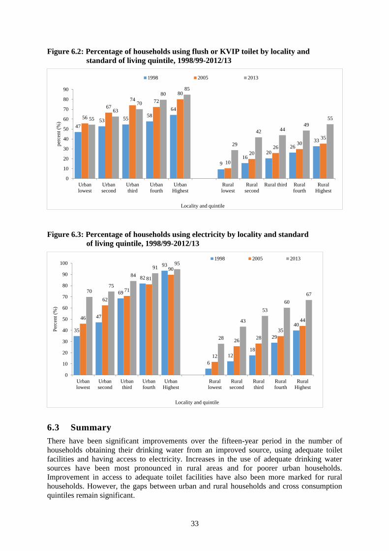
33
Figure 6.2: Percentage of households using flush or KVIP toilet by locality and
standard of living quintile, 1998/99-2012/13
Figure 6.3: Percentage of households using electricity by locality and standard
of living quintile, 1998/99-2012/13
6.3 Summary
There have been significant improvements over the fifteen-year period in the number of
households obtaining their drinking water from an improved source, using adequate toilet
facilities and having access to electricity. Increases in the use of adequate drinking water
sources have been most pronounced in rural areas and for poorer urban households.
Improvement in access to adequate toilet facilities have also been more marked for rural
households. However, the gaps between urban and rural households and cross consumption
quintiles remain significant.
47 53 55
58
64
9
16 20
26
33
56
67
74 72
80
10
20 26
30 35
55
63
70
80 85
29
42 44 49
55
0
10
20
30
40
50
60
70
80
90
Urban
lowest
Urban
second
Urban
third
Urban
fourth
Urban
Highest
Rural
lowest
Rural
second
Rural third Rural
fourth
Rural
Highest
per
cen
t (%
)
Locality and quintile
1998 2005 2013
35
47
69
82
93
6
12 18
29
40
46
62
71
81
90
12
26 28
35
44
70 75
84
91 95
28
43
53
60
67
0
10
20
30
40
50
60
70
80
90
100
Urban
lowest
Urban
second
Urban
third
Urban
fourth
Urban
Highest
Rural
lowest
Rural
second
Rural
third
Rural
fourth
Rural
Highest
Per
cen
t (%
)
Locality and quintile
1998 2005 2013

34
CHAPTER SEVEN
HUMAN DEVELOPMENT
7.1 Introduction
Along with access to services which were examined in the previous section, education and
health are also considered “basic needs” and should be seen as complementary to the
consumption-based welfare indicator. They have some of the characteristics of public goods
and are conceptually difficult to measure in monetary terms.
The health status of people is a strong determinant of their quality of life, level of
productivity and longevity. According to the World Health Organization (WHO), health is a
state of complete physical, mental and social well-being and not merely the absence of
disease or infirmity. Education has been identified as an important tool in providing people
with the basic knowledge, skills and the competencies to improve their standard of living and
quality of life. Thus, the health and the educational status of the people are directly linked to
the general state of development of a country. It is, therefore, not surprising that health and
education issues have featured prominently in the UN Human Development Index as well as
in the Millennium Development Goals. In the GLSS, information on the utilization of health
and education facilities was collected from the sampled households.
7.2 Access to health services
The information presented here covers the use of health facilities by individuals who
considered themselves to have been ill or injured in the two weeks preceding the interview.
Respondents were asked whether they consulted a health practitioner when ill or injured.
Figure 7.1 shows the percentage of individuals ill or injured who consulted a doctor by
locality and standard of living quintile. The percentage of ill or injured that consulted a doctor
has risen over the period 2005/06 to 2012/13 across all localities and quintiles. In the lowest
urban quintile the percentage who consulted a doctor rose to 34 percent from 22 percent over
the 7-year period; among the middle quintile this increased from 37 percent to 44 percent and
among the two top quintiles from 35 percent to 41 percent and 42 percent to 49 percent
respectively. In rural areas, the percentage who consulted a doctor increased systematically
over the 15 years from 1998/99, though the percentage change within quintiles between 2005
and 2013 was more noticeable, benefiting both the rich as well as the poor. Nationally, the
percentage of ill or injured individuals who did not consult any health personnel has also
declined (40.6% to 33.8). Across localities, however, the proportion of such individuals was
observed to have increased in urban savannah (Table A4.1).
Consultation with a pharmacist/chemical seller increased sharply between 1998/99 and
2005/06 for both urban and rural areas and all quintiles. However, in the last 7 years the
proportion consulting this group of health workers declined across rural and urban areas and
all quintiles. This may, to some extent, reflect the increased consultation with doctors over
the same period (Figure 7.2).

35
Figure 7.1: Percentage of ill or injured individuals that consulted a doctor
by locality and standard of living quintile, 1998/99-2012/13
Figure 7.2: Percentage of ill or injured individuals that consulted a pharmacist/
chemical seller by locality and standard of living quintile, 1998/99-2012/13
Figure 7.3 shows the percentage of ill or injured individuals who consulted in a hospital. The
Figure reveals that by 2012/13, 24 percent of the poorest urban households consulted in
hospital when ill or injured, an increase from 20 percent in 2005/06. Apart from the second
quintile in urban areas, all groups showed increases in consultation since 2005/06. Despite
these increases, there still remain large differences in the proportions consulting at a hospital
between the lowest and highest quintiles (24% and 35% respectively in urban areas; 15% and
26% in rural areas).
23
18
26
35
41
6
11 14
16
23 22
35 37 35
42
11
15 16
20
28
35 37
44
41
49
21
27 26
30 31
0
10
20
30
40
50
60
Urban
lowest
Urban
second
Urban
third
Urban
fourth
Urban
Highest
Rural
lowest
Rural
second
Rural third Rural
fourth
Rural
Highest
Per
cen
t (%
)
Locality and Quintile
1998/99 2005/06 2012/13
2 3
1
5
9
1 1 0 1
3
37
22
28
23
14
19
21
18
21 20
14 15 14
22
14 13
15 17
14
17
0
5
10
15
20
25
30
35
40
Urban
lowest
Urban
second
Urban
third
Urban
fourth
Urban
Highest
Rural
lowest
Rural
second
Rural
third
Rural
fourth
Rural
Highest
Per
cen
t (%
)
Locality and Quintile
1998/99 2005/06 2012/13
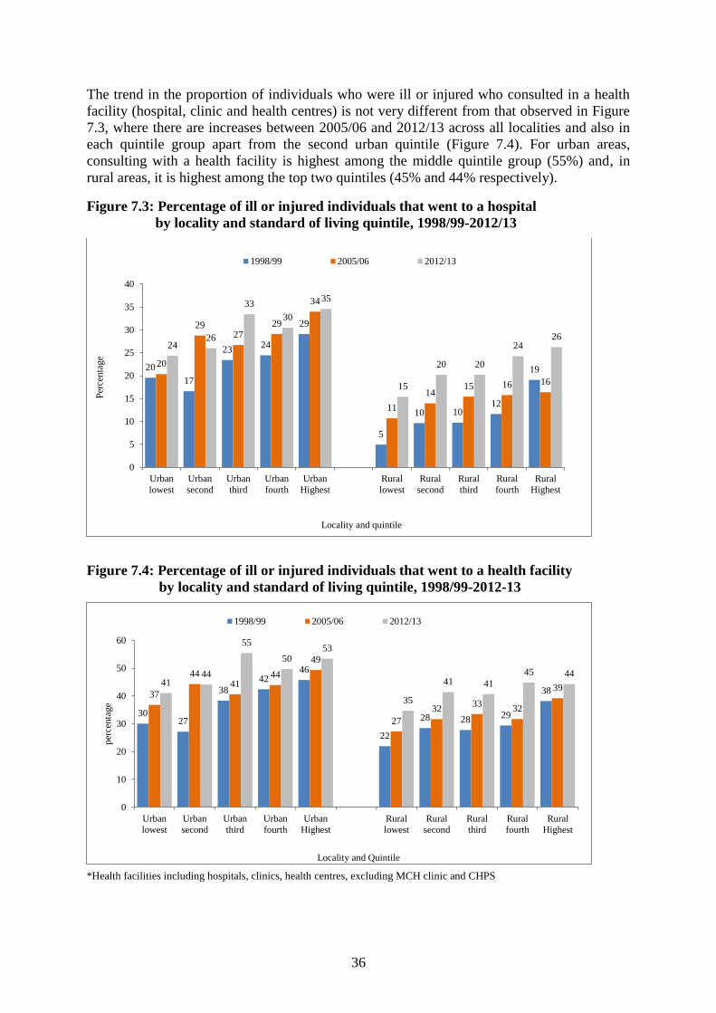
36
The trend in the proportion of individuals who were ill or injured who consulted in a health
facility (hospital, clinic and health centres) is not very different from that observed in Figure
7.3, where there are increases between 2005/06 and 2012/13 across all localities and also in
each quintile group apart from the second urban quintile (Figure 7.4). For urban areas,
consulting with a health facility is highest among the middle quintile group (55%) and, in
rural areas, it is highest among the top two quintiles (45% and 44% respectively).
Figure 7.3: Percentage of ill or injured individuals that went to a hospital
by locality and standard of living quintile, 1998/99-2012/13
Figure 7.4: Percentage of ill or injured individuals that went to a health facility
by locality and standard of living quintile, 1998/99-2012-13
*Health facilities including hospitals, clinics, health centres, excluding MCH clinic and CHPS
20
17
23 24
29
5
10 10 12
19 20
29 27
29
34
11
14 15 16 16
24 26
33
30
35
15
20 20
24 26
0
5
10
15
20
25
30
35
40
Urban
lowest
Urban
second
Urban
third
Urban
fourth
Urban
Highest
Rural
lowest
Rural
second
Rural
third
Rural
fourth
Rural
Highest
Per
cen
tage
Locality and quintile
1998/99 2005/06 2012/13
30 27
38
42 46
22
28 28 29
38 37
44 41
44
49
27
32 33
32
39 41
44
55
50 53
35
41 41
45 44
0
10
20
30
40
50
60
Urban
lowest
Urban
second
Urban
third
Urban
fourth
Urban
Highest
Rural
lowest
Rural
second
Rural
third
Rural
fourth
Rural
Highest
per
cen
tage
Locality and Quintile
1998/99 2005/06 2012/13

37
7.3 Access to education
School attendance rates are input indicators used by stakeholders nationally and
internationally to measure performance in the educational sector. In Ghana, school attendance
has increased consistently and appreciably over time, although it has stagnated in recent
years. The focus of this chapter is to assess school attendance at three levels: Primary, Junior
High School (JHS) and Senior High School (SHS). They were examined in terms of net and
gross school attendance rates, quintiles and localities.
Figure 7.5 shows the Net Attendance Rate (NAR5) for primary school by locality and sex. It
is generally high with marginal fluctuations across the localities except in the rural Savannah
where the rates are much lower. There is little difference in NAR between 2005/06 and
2012/13, with some areas experiencing a marginal increase and others a marginal decrease.
While NAR remains the lowest among the rural savannah, the largest increases in NAR
occurred in this area (15% points for girls, 12% points for boys). Figure 7.6 shows NAR by
quintile and sex. For both boys and girls, NAR increases with rising quintile, from 62
percent in the first quintile to 84 percent for boys and 82 percent for girls in the fifth quintile.
The rate is almost at parity for both sexes and the quintile groups over the period 2005/06 and
2012/13. The largest increases in NAR over the 7 year period are seen in the lowest quintiles
for both boys and girls, whereas NAR has stagnated in the higher quintiles.
Figure 7.5: Net primary school attendance ratio by sex and locality, 2005/06-2012/13
5 Net Attendance Rate (NAR) Net attendance rates of children at Primary, JHS and SHS is the number of children of official schooling
age (as defined by Ghana Education Service) who are attending Primary, JHS and SHS as a percentage of the total children of the official
school age population.
85 84
77
67 70 72
51
83 82 82
68 66 71
48
88
74
80 77
68 71
63
81 78
83 77
66
72
63
0
10
20
30
40
50
60
70
80
90
100
Accra(GAMA)
UrbanCoastal
UrbanForest
UrbanSavannah
RuralCoastal
RuralForest
RuralSavannah
Accra(GAMA)
UrbanCoastal
UrbanForest
UrbanSavannah
RuralCoastal
RuralForest
RuralSavannah
Net
att
end
ance
rat
e
Boys Girls
2005/06 2012/13
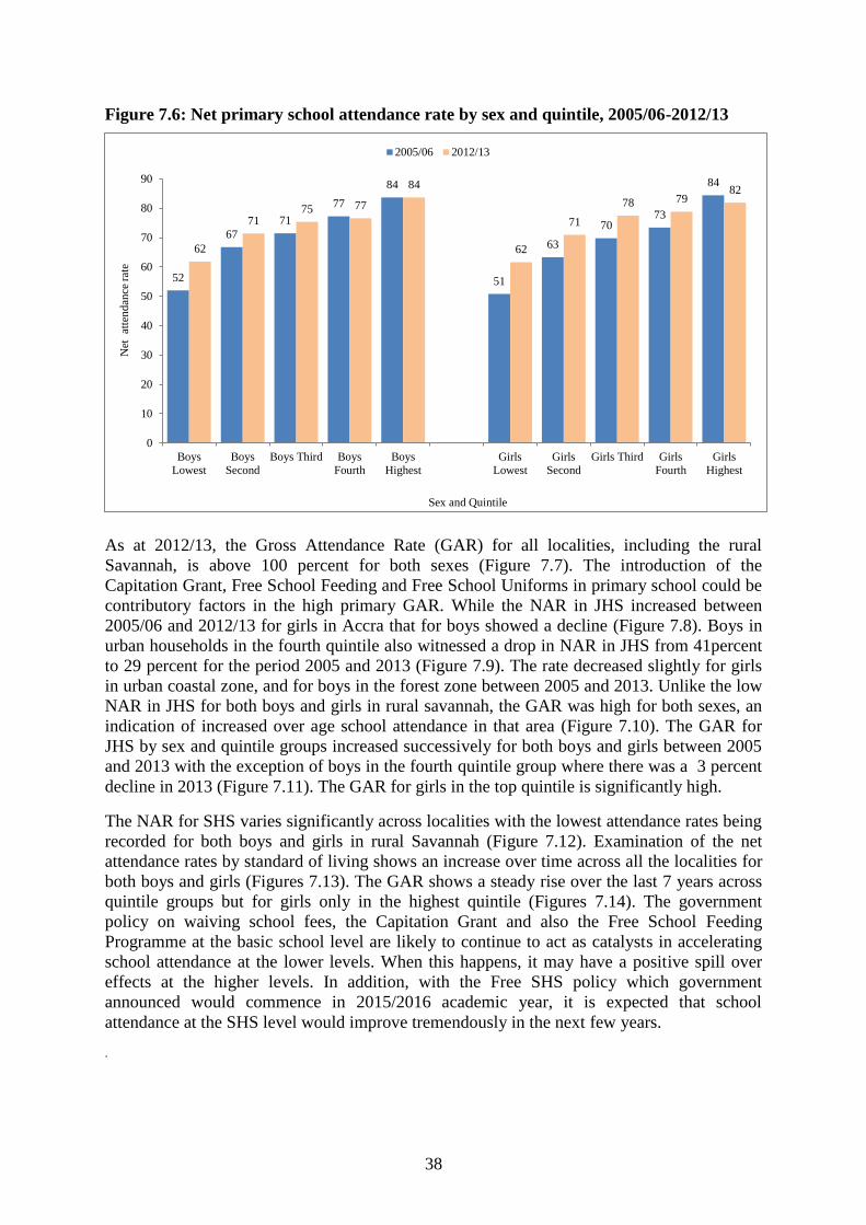
38
Figure 7.6: Net primary school attendance rate by sex and quintile, 2005/06-2012/13
As at 2012/13, the Gross Attendance Rate (GAR) for all localities, including the rural
Savannah, is above 100 percent for both sexes (Figure 7.7). The introduction of the
Capitation Grant, Free School Feeding and Free School Uniforms in primary school could be
contributory factors in the high primary GAR. While the NAR in JHS increased between
2005/06 and 2012/13 for girls in Accra that for boys showed a decline (Figure 7.8). Boys in
urban households in the fourth quintile also witnessed a drop in NAR in JHS from 41percent
to 29 percent for the period 2005 and 2013 (Figure 7.9). The rate decreased slightly for girls
in urban coastal zone, and for boys in the forest zone between 2005 and 2013. Unlike the low
NAR in JHS for both boys and girls in rural savannah, the GAR was high for both sexes, an
indication of increased over age school attendance in that area (Figure 7.10). The GAR for
JHS by sex and quintile groups increased successively for both boys and girls between 2005
and 2013 with the exception of boys in the fourth quintile group where there was a 3 percent
decline in 2013 (Figure 7.11). The GAR for girls in the top quintile is significantly high.
The NAR for SHS varies significantly across localities with the lowest attendance rates being
recorded for both boys and girls in rural Savannah (Figure 7.12). Examination of the net
attendance rates by standard of living shows an increase over time across all the localities for
both boys and girls (Figures 7.13). The GAR shows a steady rise over the last 7 years across
quintile groups but for girls only in the highest quintile (Figures 7.14). The government
policy on waiving school fees, the Capitation Grant and also the Free School Feeding
Programme at the basic school level are likely to continue to act as catalysts in accelerating
school attendance at the lower levels. When this happens, it may have a positive spill over
effects at the higher levels. In addition, with the Free SHS policy which government
announced would commence in 2015/2016 academic year, it is expected that school
attendance at the SHS level would improve tremendously in the next few years.
.
52
67
71
77
84
51
63
70 73
84
62
71 75 77
84
62
71
78 79 82
0
10
20
30
40
50
60
70
80
90
Boys
Lowest
Boys
Second
Boys Third Boys
Fourth
Boys
Highest
Girls
Lowest
Girls
Second
Girls Third Girls
Fourth
Girls
Highest
Net
at
ten
dan
ce r
ate
Sex and Quintile
2005/06 2012/13

39
Figure 7.7: Gross primary school attendance rate by sex and locality, 2005/06-2012/13
Figure 7.8: Net JHS school attendance rate by sex and locality, 2005/06-2012/13
113
127 115 122
133
116
91
116 115 116 118 118
111
83
120
111
119 123 122 122
116 112
129
120 125
111 114
108
0
20
40
60
80
100
120
140
160
Accra(GAMA)
UrbanCoastal
UrbanForest
UrbanSavannah
RuralCoastal
RuralForest
RuralSavannah
Accra(GAMA)
UrbanCoastal
UrbanForest
UrbanSavannah
RuralCoastal
RuralForest
RuralSavannah
Gro
ss a
tten
dan
ce r
ate
Boys Girls
2005/06 2012/13
55
39 39
24
16
24
7
47 49
33
17 19
23
10
49
29
38
27
20 18
11
53
35 36
30
20
25
12
0
10
20
30
40
50
60
Accra
(GAMA)
Urban
Coastal
Urban
Forest
Urban
Savannah
Rural
Coastal
Rural
Forest
Rural
Savannah
Accra
(GAMA)
Urban
Coastal
Urban
Forest
Urban
Savannah
Rural
Coastal
Rural
Forest
Rural
Savannah
Net
att
end
ance
rat
e
Boys Girls
2005/06 2012/13
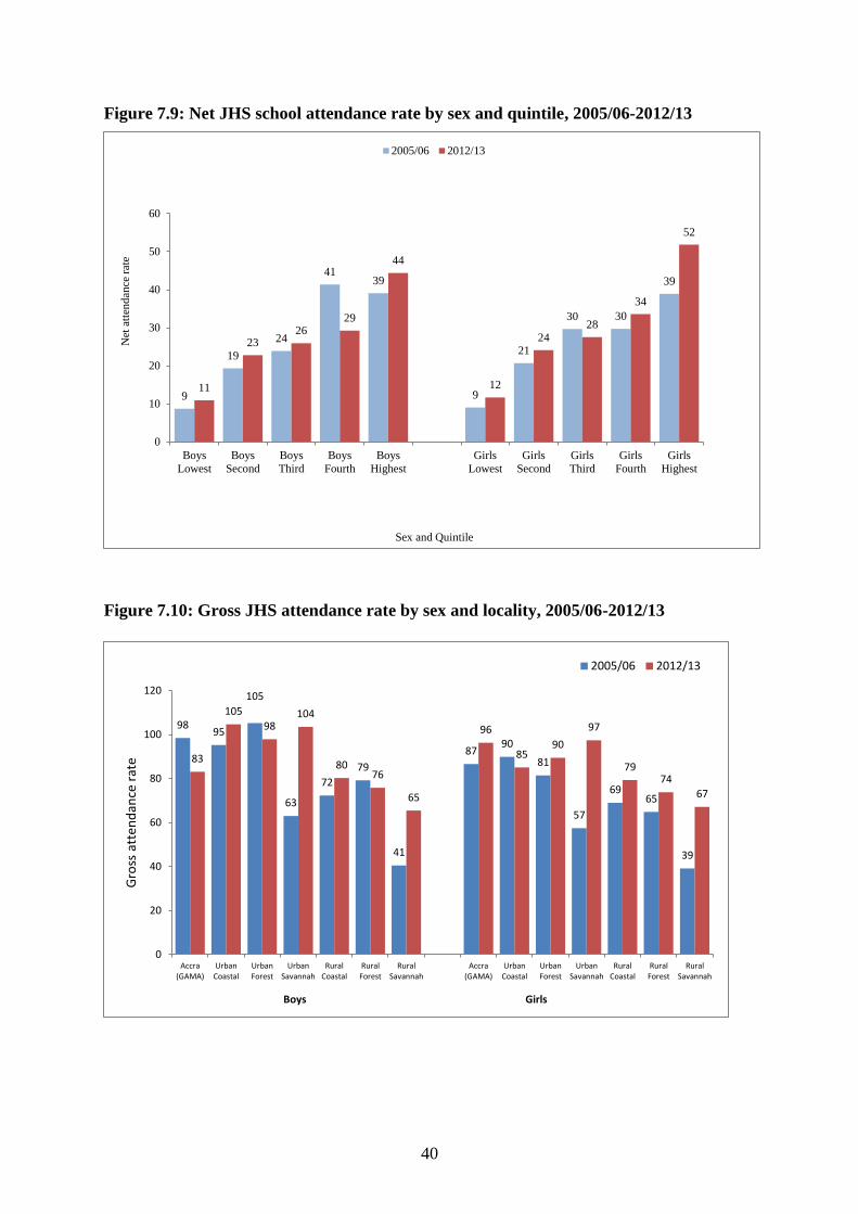
40
Figure 7.9: Net JHS school attendance rate by sex and quintile, 2005/06-2012/13
Figure 7.10: Gross JHS attendance rate by sex and locality, 2005/06-2012/13
9
19
24
41 39
9
21
30 30
39
11
23 26
29
44
12
24 28
34
52
0
10
20
30
40
50
60
Boys
Lowest
Boys
Second
Boys
Third
Boys
Fourth
Boys
Highest
Girls
Lowest
Girls
Second
Girls
Third
Girls
Fourth
Girls
Highest
Net
att
end
ance
rat
e
Sex and Quintile
2005/06 2012/13
98 95
105
63
72
79
41
87 90
81
57
69 65
39
83
105
98 104
80 76
65
96
85 90
97
79 74
67
0
20
40
60
80
100
120
Accra(GAMA)
UrbanCoastal
UrbanForest
UrbanSavannah
RuralCoastal
RuralForest
RuralSavannah
Accra(GAMA)
UrbanCoastal
UrbanForest
UrbanSavannah
RuralCoastal
RuralForest
RuralSavannah
Gro
ss a
tten
dan
ce r
ate
Boys Girls
2005/06 2012/13

41
Figure 7.11: Gross JHS school attendance rate by sex and quintile, 2005/06-2012/13
Figure 7.12: Net SHS school attendance rate by sex and locality, 2005/06-2012/13
47
73
78
98
79
39
67 62
77
84
68
85 81
89 91
64
81 78
89
107
0
20
40
60
80
100
120
Boys
Lowest
Boys
Second
Boys Third Boys
Fourth
Boys
Highest
Girls
Lowest
Girls
Second
Girls Third Girls
Fourth
Girls
Highest
Gro
ss a
tten
dan
ce r
ate
Sex and Quintile
2005/06 2012/13
34
28
23
10
4
8
3
36
24
18 18
5 7
2
37
19
21
13
7 7 6
33
24
19
10
5
10
5
0
5
10
15
20
25
30
35
40
Accra
(GAMA)
Urban
Coastal
Urban
Forest
Urban
Savannah
Rural
Coastal
Rural
Forest
Rural
Savannah
Accra
(GAMA)
Urban
Coastal
Urban
Forest
Urban
Savannah
Rural
Coastal
Rural
Forest
Rural
Savannah
Net
att
end
ance
rat
e
Boys Girls
2005/06 2012/13

42
Figure 7.13: Net SHS school attendance rate by sex and quintile, 2005/06-2012/13
Figure 7.14: Gross SSS school attendance rate by sex and quintile, 2005/06-2012/13
2
6
13
17
38
2
5
16
18
25
4
8
13
22
34
4
7
13
21
27
0
5
10
15
20
25
30
35
40
Boys
Lowest
Boys
Second
Boys Third Boys
Fourth
Boys
Highest
Girls
Lowest
Girls
Second
Girls Third Girls
Fourth
Girls
Highest
Net
att
end
ance
rat
e
Sex and Quintile
2005/06 2012/13
13 18
35 42
80
10 15
31
45
54
25
46 50
78
110
22 27
47
60
67
0
20
40
60
80
100
120
Boys
Lowest
Boys
Second
Boys
Third
Boys
Fourth
Boys
Highest
Girls
Lowest
Girls
Second
Girls Third Girls
Fourth
Girls
Highest
Gro
ss a
tten
dan
ce r
ate
Sex and Quintile
2005/06 2012/13

43
7.4 Summary
The survey period 2005/06 to 2012/13 has seen increased rates of access to a range of health
services. However, disparities remain between urban and rural areas and between quintile
groups within those areas. Compared to 1998/99 and 2005/06, individuals are more likely
now to consult doctors and visit health facilities. Consultation with pharmacists or chemical
sellers when ill or injured has decreased. The percentage of individuals ill or injured who did
not consult any health practitioner has also declined. This pattern is observed in all income
groups in both rural and urban areas.
In terms of education, school attendance rates in primary, JHS and SHS have improved over
this seven-year period. The savannah areas are still reporting the lowest school attendance
rates. The increases in net school attendance rates at the JHS level have been much higher for
girls than boys, but are still below those for boys and the reverse holds for SHS. Even with
these increases, NAR at SHS are much lower than at the primary and JHS levels, and
especially so in rural areas.

44
CHAPTER EIGHT
CONCLUSION
Ghana achieved positive economic growth in 1991 and by 2007, the country had become a
lower-middle income country. The decline in poverty observed over the years have largely
been attributed to this growth but to what extent have Ghanaian households and communities
benefited from this growth and which groups have benefited most? These questions can only
be answered by measuring progress in the welfare of the population.
The Ghana Living Standards Survey (GLSS) is among the series of household surveys that
have been conducted by the Ghana Statistical Service (GSS) since 1987 to generate data for
the measurement of the well-being of the Ghanaian population. Results from the previous
five rounds of the survey have provided a wealth of information for understanding living
conditions in the country, and for planning and monitoring the impact of developmental
policies and programmes on the lives of the people.
The sixth round (GLSS6) was initiated in October 2012 and completed in October 2013.
This survey covered a wide range of indicators including education, health, employment and
time use, household assets, and housing conditions, among others. Interviews were conducted
among 18,000 households in 1,200 enumeration areas selected across the entire country.
The results of the survey indicate that Ghana has made an enormous amount of progress since
the previous GLSS in 2006. More importantly, the country has met the first MDG target of
halving poverty between 1990 and 2015, reducing it from 51.7 percent of the population in
1992 to 24.2 percent in 2013. Based on the same consumption basket, the proportion of
people living in poverty declined from 31.9 percent in 2005/06 to 24.2 percent in 2012/13,
the number of people living in poverty declined from 7 million to 6.4 million. Similarly, the
proportion of people living in extreme poverty (those unable to meet their basic food needs)
declined from 16.5 percent in 2006 to 8.4 percent in 2013. This means that the number of
people living in extreme poverty has reduced from 3.6 million in 2006 to 2.2 million in 2013.
Regional analysis of the data suggests that poverty has been reduced in all regions, except in
the Eastern Region.
Progress has also been made in many important areas such as education, healthcare and
infrastructure, which clearly reflects in the gains made in reducing poverty among various
population subgroups, for example, the educated. Generally, poverty remains a rural
phenomenon, with those in rural Savannah being mostly affected. At the regional level, the
incidence of poverty is largely concentrated in the three northern regions. Greater Accra, on
the other hand, is the least poor.
A key area that continues to worsen and is a clear source of concern is that of equity.
Ghana’s inequality measure, the Gini Coefficient, has risen from 41.9 in 2005/06 to 42.3 in
2012/13, an indication that increasingly, income is shared inequitably across the population.
This level of inequality has adverse implications towards Government’s efforts at reducing
poverty in the country.

45
AP
PE
ND
IX
TA
BL
ES
AN
D
ME
TH
OD
OL
OG
Y
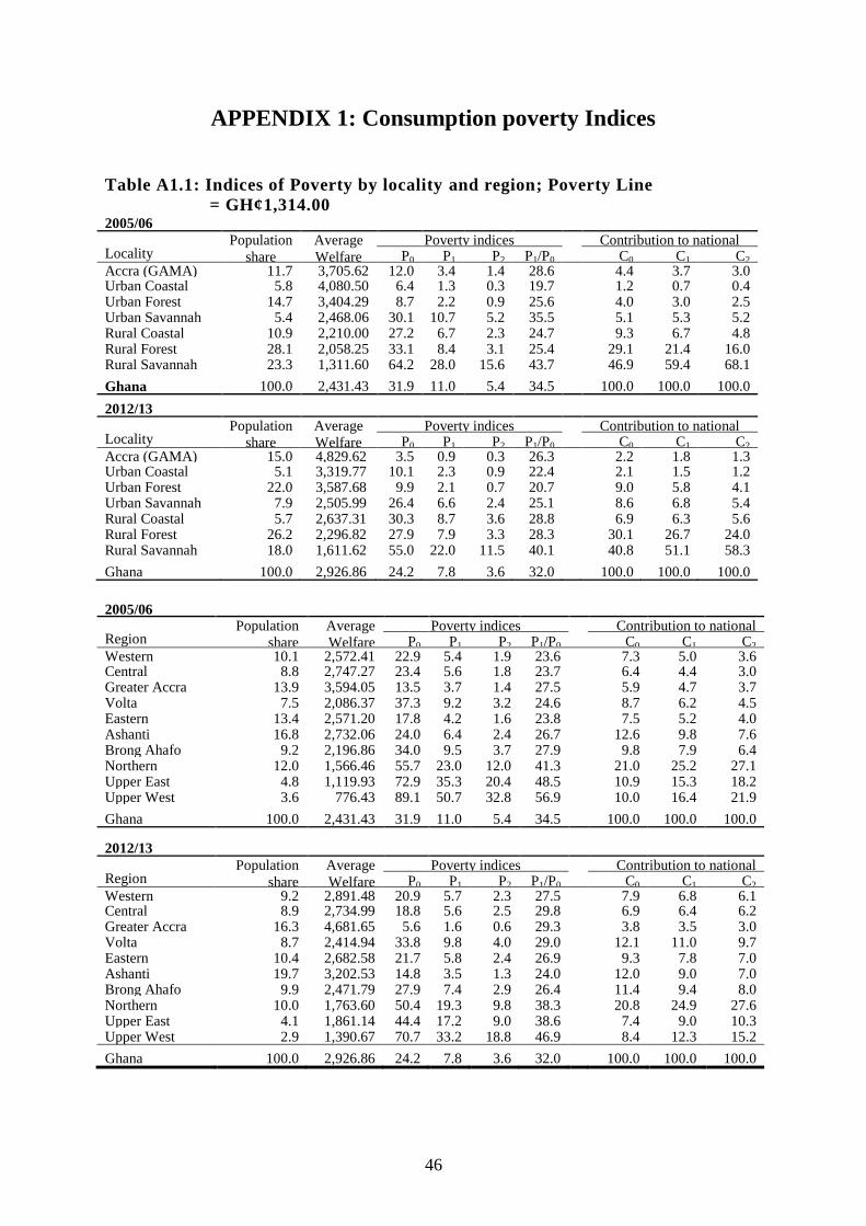
46
APPENDIX 1: Consumption poverty Indices
Table A1.1: Indices of Poverty by locality and region; Poverty Line
= GH¢1,314.00 2005/06
Locality
Population
share
Average
Welfare
Poverty indices Contribution to national
poverty P0 P1 P2 P1/P0 C0 C1 C2 Accra (GAMA) 11.7 3,705.62 12.0 3.4 1.4 28.6
4.4 3.7 3.0
Urban Coastal 5.8 4,080.50 6.4 1.3 0.3 19.7
1.2 0.7 0.4 Urban Forest 14.7 3,404.29 8.7 2.2 0.9 25.6
4.0 3.0 2.5
Urban Savannah 5.4 2,468.06 30.1 10.7 5.2 35.5
5.1 5.3 5.2 Rural Coastal 10.9 2,210.00 27.2 6.7 2.3 24.7
9.3 6.7 4.8
Rural Forest 28.1 2,058.25 33.1 8.4 3.1 25.4
29.1 21.4 16.0 Rural Savannah 23.3 1,311.60 64.2 28.0 15.6 43.7
46.9 59.4 68.1
Ghana 100.0 2,431.43 31.9 11.0 5.4 34.5 100.0 100.0 100.0
2012/13
Locality Population
share
Average
Welfare
Poverty indices Contribution to national
poverty P0 P1 P2 P1/P0 C0 C1 C2 Accra (GAMA) 15.0 4,829.62 3.5 0.9 0.3 26.3
2.2 1.8 1.3
Urban Coastal 5.1 3,319.77 10.1 2.3 0.9 22.4
2.1 1.5 1.2 Urban Forest 22.0 3,587.68 9.9 2.1 0.7 20.7
9.0 5.8 4.1
Urban Savannah 7.9 2,505.99 26.4 6.6 2.4 25.1
8.6 6.8 5.4 Rural Coastal 5.7 2,637.31 30.3 8.7 3.6 28.8
6.9 6.3 5.6
Rural Forest 26.2 2,296.82 27.9 7.9 3.3 28.3
30.1 26.7 24.0 Rural Savannah 18.0 1,611.62 55.0 22.0 11.5 40.1
40.8 51.1 58.3
Ghana 100.0 2,926.86 24.2 7.8 3.6 32.0 100.0 100.0 100.0
2005/06
Region
Population
share
Average
Welfare
Poverty indices Contribution to national
poverty P0 P1 P2 P1/P0 C0 C1 C2 Western 10.1 2,572.41 22.9 5.4 1.9 23.6
7.3 5.0 3.6
Central 8.8 2,747.27 23.4 5.6 1.8 23.7
6.4 4.4 3.0 Greater Accra 13.9 3,594.05 13.5 3.7 1.4 27.5
5.9 4.7 3.7
Volta 7.5 2,086.37 37.3 9.2 3.2 24.6
8.7 6.2 4.5 Eastern 13.4 2,571.20 17.8 4.2 1.6 23.8
7.5 5.2 4.0
Ashanti 16.8 2,732.06 24.0 6.4 2.4 26.7
12.6 9.8 7.6 Brong Ahafo 9.2 2,196.86 34.0 9.5 3.7 27.9
9.8 7.9 6.4
Northern 12.0 1,566.46 55.7 23.0 12.0 41.3
21.0 25.2 27.1 Upper East 4.8 1,119.93 72.9 35.3 20.4 48.5
10.9 15.3 18.2
Upper West 3.6 776.43 89.1 50.7 32.8 56.9
10.0 16.4 21.9
Ghana 100.0 2,431.43 31.9 11.0 5.4 34.5 100.0 100.0 100.0
2012/13
Region Population
share
Average
Welfare
Poverty indices Contribution to national
poverty P0 P1 P2 P1/P0 C0 C1 C2 Western 9.2 2,891.48 20.9 5.7 2.3 27.5
7.9 6.8 6.1
Central 8.9 2,734.99 18.8 5.6 2.5 29.8
6.9 6.4 6.2 Greater Accra 16.3 4,681.65 5.6 1.6 0.6 29.3
3.8 3.5 3.0
Volta 8.7 2,414.94 33.8 9.8 4.0 29.0
12.1 11.0 9.7 Eastern 10.4 2,682.58 21.7 5.8 2.4 26.9
9.3 7.8 7.0
Ashanti 19.7 3,202.53 14.8 3.5 1.3 24.0
12.0 9.0 7.0 Brong Ahafo 9.9 2,471.79 27.9 7.4 2.9 26.4
11.4 9.4 8.0
Northern 10.0 1,763.60 50.4 19.3 9.8 38.3
20.8 24.9 27.6 Upper East 4.1 1,861.14 44.4 17.2 9.0 38.6
7.4 9.0 10.3
Upper West 2.9 1,390.67 70.7 33.2 18.8 46.9
8.4 12.3 15.2
Ghana 100.0 2,926.86 24.2 7.8 3.6 32.0 100.0 100.0 100.0
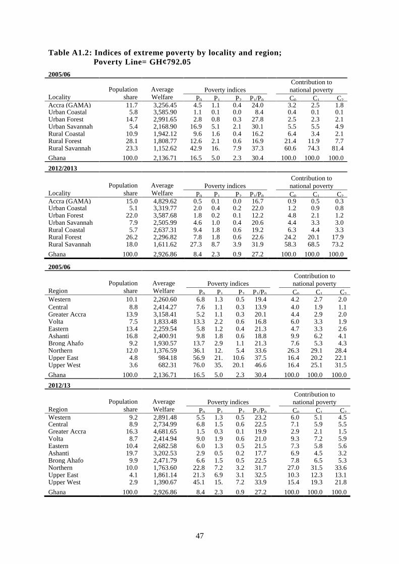
47
Table A1.2: Indices of extreme poverty by locality and region;
Poverty Line= GH¢792.05
2005/06
Locality
Population
share
Average
Welfare Poverty indices
Contribution to
national poverty
P0 P1 P2 P1/P0 C0 C1 C2 Accra (GAMA) 11.7 3,256.45 4.5 1.1 0.4 24.0
3.2 2.5 1.8
Urban Coastal 5.8 3,585.90 1.1 0.1 0.0 8.4
0.4 0.1 0.1 Urban Forest 14.7 2,991.65 2.8 0.8 0.3 27.8
2.5 2.3 2.1
Urban Savannah 5.4 2,168.90 16.9 5.1 2.1 30.1
5.5 5.5 4.9 Rural Coastal 10.9 1,942.12 9.6 1.6 0.4 16.2
6.4 3.4 2.1
Rural Forest 28.1 1,808.77 12.6 2.1 0.6 16.9
21.4 11.9 7.7 Rural Savannah 23.3 1,152.62 42.9 16.
0
7.9 37.3
60.6 74.3 81.4
Ghana 100.0 2,136.71 16.5 5.0 2.3 30.4 100.0 100.0 100.0
2012/2013
Locality
Population
share
Average
Welfare Poverty indices
Contribution to
national poverty
P0 P1 P2 P1/P0 C0 C1 C2 Accra (GAMA) 15.0 4,829.62 0.5 0.1 0.0 16.7
0.9 0.5 0.3
Urban Coastal 5.1 3,319.77 2.0 0.4 0.2 22.0
1.2 0.9 0.8 Urban Forest 22.0 3,587.68 1.8 0.2 0.1 12.2
4.8 2.1 1.2
Urban Savannah 7.9 2,505.99 4.6 1.0 0.4 20.6
4.4 3.3 3.0 Rural Coastal 5.7 2,637.31 9.4 1.8 0.6 19.2
6.3 4.4 3.3
Rural Forest 26.2 2,296.82 7.8 1.8 0.6 22.6
24.2 20.1 17.9 Rural Savannah 18.0 1,611.62 27.3 8.7 3.9 31.9
58.3 68.5 73.2
Ghana 100.0 2,926.86 8.4 2.3 0.9 27.2 100.0 100.0 100.0
2005/06
Region
Population
share
Average
Welfare Poverty indices
Contribution to
national poverty
P0 P1 P2 P1/P0 C0 C1 C2 Western 10.1 2,260.60 6.8 1.3 0.5 19.4
4.2 2.7 2.0
Central 8.8 2,414.27 7.6 1.1 0.3 13.9
4.0 1.9 1.1 Greater Accra 13.9 3,158.41 5.2 1.1 0.3 20.1
4.4 2.9 2.0
Volta 7.5 1,833.48 13.3 2.2 0.6 16.8
6.0 3.3 1.9 Eastern 13.4 2,259.54 5.8 1.2 0.4 21.3
4.7 3.3 2.6
Ashanti 16.8 2,400.91 9.8 1.8 0.6 18.8
9.9 6.2 4.1 Brong Ahafo 9.2 1,930.57 13.7 2.9 1.1 21.3
7.6 5.3 4.3
Northern 12.0 1,376.59 36.1 12.
1
5.4 33.6
26.3 29.1 28.4 Upper East 4.8 984.18 56.9 21.
3
10.6 37.5
16.4 20.2 22.1 Upper West 3.6 682.31 76.0 35.
4
20.1 46.6
16.4 25.1 31.5
Ghana 100.0 2,136.71 16.5 5.0 2.3 30.4 100.0 100.0 100.0
2012/13
Region
Population
share
Average
Welfare Poverty indices
Contribution to
national poverty
P0 P1 P2 P1/P0 C0 C1 C2 Western 9.2 2,891.48 5.5 1.3 0.5 23.2
6.0 5.1 4.5
Central 8.9 2,734.99 6.8 1.5 0.6 22.5
7.1 5.9 5.5 Greater Accra 16.3 4,681.65 1.5 0.3 0.1 19.9
2.9 2.1 1.5
Volta 8.7 2,414.94 9.0 1.9 0.6 21.0
9.3 7.2 5.9 Eastern 10.4 2,682.58 6.0 1.3 0.5 21.5
7.3 5.8 5.6
Ashanti 19.7 3,202.53 2.9 0.5 0.2 17.7
6.9 4.5 3.2 Brong Ahafo 9.9 2,471.79 6.6 1.5 0.5 22.5
7.8 6.5 5.3
Northern 10.0 1,763.60 22.8 7.2 3.2 31.7
27.0 31.5 33.6 Upper East 4.1 1,861.14 21.3 6.9 3.1 32.5
10.3 12.3 13.1
Upper West 2.9 1,390.67 45.1 15.
3
7.2 33.9
15.4 19.3 21.8
Ghana 100.0 2,926.86 8.4 2.3 0.9 27.2 100.0 100.0 100.0
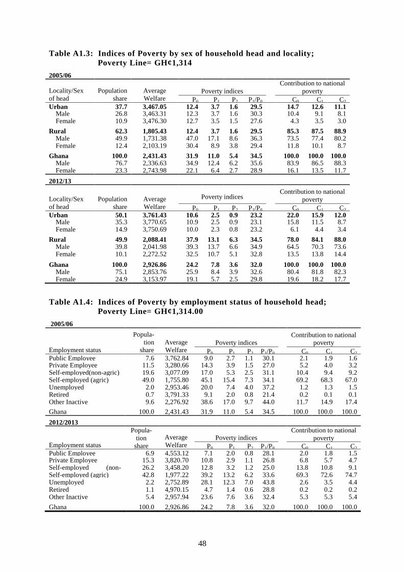
48
Table A1.3: Indices of Poverty by sex of household head and locality;
Poverty Line= GH¢1,314
2005/06
Locality/Sex
of head
Population
share
Average
Welfare
Poverty indices
Contribution to national
poverty
P0 P1 P2 P1/P0 C0 C1 C2 Urban 37.7 3,467.05 12.4 3.7 1.6 29.5
14.7 12.6 11.1
Male 26.8 3,463.31 12.3 3.7 1.6 30.3
10.4 9.1 8.1 Female 10.9 3,476.30 12.7 3.5 1.5 27.6
4.3 3.5 3.0
Rural 62.3 1,805.43 12.4 3.7 1.6 29.5
85.3 87.5 88.9 Male 49.9 1,731.38 47.0 17.1 8.6 36.3
73.5 77.4 80.2
Female 12.4 2,103.19 30.4 8.9 3.8 29.4
11.8 10.1 8.7
Ghana 100.0 2,431.43 31.9 11.0 5.4 34.5
100.0 100.0 100.0 Male 76.7 2,336.63 34.9 12.4 6.2 35.6
83.9 86.5 88.3
Female 23.3 2,743.98 22.1 6.4 2.7 28.9 16.1 13.5 11.7
2012/13
Locality/Sex
of head
Population
share
Average
Welfare
Poverty indices
Contribution to national
poverty
P0 P1 P2 P1/P0 C0 C1 C2 Urban 50.1 3,761.43 10.6 2.5 0.9 23.2
22.0 15.9 12.0
Male 35.3 3,770.65 10.9 2.5 0.9 23.1
15.8 11.5 8.7 Female 14.9 3,750.69 10.0 2.3 0.8 23.2
6.1 4.4 3.4
Rural 49.9 2,088.41 37.9 13.1 6.3 34.5
78.0 84.1 88.0 Male 39.8 2,041.98 39.3 13.7 6.6 34.9
64.5 70.3 73.6
Female 10.1 2,272.52 32.5 10.7 5.1 32.8
13.5 13.8 14.4
Ghana 100.0 2,926.86 24.2 7.8 3.6 32.0
100.0 100.0 100.0 Male 75.1 2,853.76 25.9 8.4 3.9 32.6
80.4 81.8 82.3
Female 24.9 3,153.97 19.1 5.7 2.5 29.8 19.6 18.2 17.7
Table A1.4: Indices of Poverty by employment status of household head;
Poverty Line= GH¢1,314.00
2005/06
Employment status
Popula-
tion
share
Average
Welfare Poverty indices
Contribution to national
poverty
P0 P1 P2 P1/P0 C0 C1 C2 Public Employee 7.6 3,762.84 9.0 2.7 1.1 30.1
2.1 1.9 1.6
Private Employee 11.5 3,280.66 14.3 3.9 1.5 27.0
5.2 4.0 3.2 Self-employed(non-agric) 19.6 3,077.09 17.0 5.3 2.5 31.1
10.4 9.4 9.2
Self-employed (agric) 49.0 1,755.80 45.1 15.4 7.3 34.1
69.2 68.3 67.0 Unemployed 2.0 2,953.46 20.0 7.4 4.0 37.2
1.2 1.3 1.5
Retired 0.7 3,791.33 9.1 2.0 0.8 21.4
0.2 0.1 0.1 Other Inactive 9.6 2,276.92 38.6 17.0 9.7 44.0
11.7 14.9 17.4
Ghana 100.0 2,431.43 31.9 11.0 5.4 34.5 100.0 100.0 100.0
2012/2013
Employment status
Popula-
tion
share
Average
Welfare Poverty indices
Contribution to national
poverty
P0 P1 P2 P1/P0 C0 C1 C2 Public Employee 6.9 4,553.12 7.1 2.0 0.8 28.1
2.0 1.8 1.5
Private Employee 15.3 3,820.70 10.8 2.9 1.1 26.8
6.8 5.7 4.7 Self-employed (non-
agric)
26.2 3,458.20 12.8 3.2 1.2 25.0
13.8 10.8 9.1 Self-employed (agric) 42.8 1,977.22 39.2 13.2 6.2 33.6
69.3 72.6 74.7
Unemployed 2.2 2,752.89 28.1 12.3 7.0 43.8
2.6 3.5 4.4 Retired 1.1 4,970.15 4.7 1.4 0.6 28.8
0.2 0.2 0.2
Other Inactive 5.4 2,957.94 23.6 7.6 3.6 32.4
5.3 5.3 5.4
Ghana 100.0 2,926.86 24.2 7.8 3.6 32.0 100.0 100.0 100.0

49
Table A1.5: Indices of extreme poverty by employment status of
household head, Poverty Line= GH¢792.05
2005/06
Employment Status
Population
share
Average
Welfare Poverty indices
Contribution to
national poverty
P0 P1 P2 P1/P0 C0 C1 C2 Public Employee 7.6 2,964.66 4.6 1.3 0.5 27.9
1.7 1.5 1.2
Private Employee 11.5 2,584.76 8.3 1.7 0.6 21.0
4.7 3.1 2.3 Self-employed (non-
agric)
19.6 2,424.37 9.2 3.0 1.4 32.4
8.9 9.1 9.1 Self-employed (agric) 49.0 1,383.36 28.5 8.8 3.9 30.8
69.2 67.3 65.0
Unemployed 2.0 2,326.97 12.2 4.7 2.5 38.9
1.2 1.5 1.7 Retired 0.7 2,987.11 2.8 1.0 0.4 34.0
0.1 0.1 0.1
Other Inactive 9.6 1,793.94 29.6 11.5 6.3 38.9
14.2 17.4 20.6
Ghana 100.0 2,136.71 16.5 5.0 2.3 30.4 100.0 100.0 100.0
2012/2013
Employment Status
Population
share
Average
Welfare Poverty indices
Contribution to
national poverty
P0 P1 P2 P1/P0 C0 C1 C2 Public Employee 6.9 4,553.12 3.5 0.9 0.3 27.3
1.6 1.4 1.1
Private Employee 15.3 3,820.70 5.1 1.2 0.4 23.1
3.5 2.7 1.9 Self-employed (non-
agric)
26.2 3,458.20 8.2 2.3 1.1 28.4
9.7 9.1 9.1 Self-employed (agric) 42.8 1,977.22 23.2 6.8 3.0 29.3
68.9 66.5 63.9
Unemployed 2.2 2,752.89 10.7 4.0 2.1 37.4
1.3 1.6 1.8 Retired 1.1 4,970.15 2.8 0.8 0.3 26.4
0.1 0.1 0.1
Other Inactive 5.4 2,957.94 25.5 9.7 5.2 38.1
14.9 18.6 22.2
Ghana 100.0 2,926.86 8.4 2.3 0.9 27.2 100.0 100.0 100.0
Table A1.6: Indices of poverty by educational level of household head;
Poverty Line= GH¢1,314
2012/13
Educational level
of head
Popula-
tion
share
Average
Welfare Poverty indices
Contribution to national
poverty
P0 P1 P2 P1/P0 C0 C1 C2 None 46.7 2,087.46 37.6 12.8 6.1 34.2
72.4 77.2 80.7
BECE 13.5 3,089.37 15.7 3.9 1.5 24.9
8.8 6.8 5.7 MSLC 21.7 3,023.27 16.2 4.5 1.8 28.1
14.5 12.7 11.0
SSS/Secondary 7.9 4,263.78 8.0 1.8 0.7 22.7
2.6 1.9 1.5 Voc/Tech/Teacher 4.7 4,267.37 5.5 1.4 0.5 24.8
1.1 0.8 0.6
Tertiary 5.4 6,268.60 3.0 0.9 0.3 28.7
0.7 0.6 0.5
Ghana 100.0 2,926.86 24.2 7.8 3.6 32.0 100.0 100.0 100.0
2005/06
Educational level
of head
Popula-
tion
share
Average
Welfare Poverty indices
Contribution to national
poverty
P0 P1 P2 P1/P0 C0 C1 C2 None 56.1 1,837.26 44.3 16.6 8.5 37.3
78.0 84.4 88.6
BECE 5.8 3,063.14 14.6 3.6 1.2 24.3
2.7 1.9 1.3 MSLC 24.4 2,602.18 21.7 5.1 1.8 23.6
16.6 11.3 8.1
SSS/Secondary 4.8 3,707.86 9.2 2.8 1.2 30.3
1.4 1.2 1.1 Voc/Tech/Teacher 6.1 3,866.58 7.2 2.0 0.8 27.9
1.4 1.1 0.9
Tertiary 2.7 6,305.03 0.3 0.1 0.0 15.2
0.0 0.0 0.0
Ghana 100.0 2,431.43 31.9 11.0 5.4 34.5 100.0 100.0 100.0

50
Table A1.7: Indices of poverty by educational level of household head;
Poverty Line= GH¢792.05
2012/13 Educational level
of head
Population
share
Average
Welfare
Poverty indices Contribution to national
poverty P0 P1 P2 P1/P0 C0 C1 C2 None 46.7 2,087.46 14.4 4.2 1.8 29.3
79.7 85.9 88.3
BECE 13.5 3,089.37 3.4 0.7 0.3 22.0
5.4 4.4 4.0 MSLC 21.7 3,023.27 4.9 0.8 0.3 17.2
12.6 7.9 6.5
SSS/Secondary 7.9 4,263.78 1.6 0.3 0.1 18.2
1.5 1.0 0.7 Voc/Tech/Teacher 4.7 4,267.37 0.6 0.2 0.1 33.5
0.4 0.4 0.4
Tertiary 5.4 6,268.60 0.7 0.1 0.0 19.8
0.5 0.3 0.2
Ghana 100 2,926.86 8.4 2.3 0.9 27.2 100.0 100.0 100.0
2005/06 Educational level
of head
Population
share
Average
Welfare
Poverty indices Contribution to national
poverty P0 P1 P2 P1/P0 C0 C1 C2 None 56.1 1,614.56 25.8 8.2 3.8 31.8
87.7 91.9 94.2
BECE 5.8 2,691.85 4.1 0.7 0.2 18.0
1.5 0.9 0.6 MSLC 24.4 2,286.76 5.9 1.1 0.4 19.4
8.7 5.6 4.0
SSS/Secondary 4.8 3,258.42 4.0 1.1 0.4 27.0
1.1 1.0 0.8 Voc/Tech/Teacher 6.1 3,397.91 2.8 0.6 0.2 20.9
1.0 0.7 0.5
Tertiary 2.7 5,540.78 0.1 0.0 0.0 5.4
0.0 0.0 0.0
Ghana 100.0 2,136.71 20.2 6.4 2.9 31.7 100.0 100.0 100.0
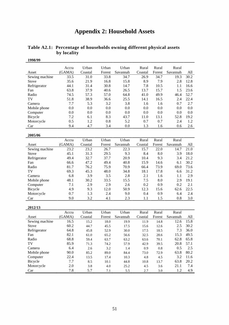
51
Appendix 2: Household Assets
Table A2.1: Percentage of households owning different physical assets
by locality
1998/99
Asset
Accra
(GAMA)
Urban
Coastal
Urban
Forest
Urban
Savannah
Rural
Coastal
Rural
Forest
Rural
Savannah All
Sewing machine 33.5 31.0 33.8 34.7 26.9 34.7 19.3 30.2
Stove 35.6 21.9 16.8 15.8 8.9 7.9 2.8 12.8
Refrigerator 44.1 31.4 30.8 14.7 7.8 10.5 1.1 16.6
Fan 63.8 37.9 40.6 26.5 13.7 15.7 1.5 23.6
Radio 74.5 57.3 57.0 64.8 41.0 49.9 46.4 52.7
TV 51.8 38.9 36.6 25.5 14.1 16.5 2.4 22.4
Camera 7.7 5.3 3.2 3.8 1.6 1.6 0.7 2.7
Mobile phone 0.0 0.0 0.0 0.0 0.0 0.0 0.0 0.0
Computer 0.0 0.0 0.0 0.0 0.0 0.0 0.0 0.0
Bicycle 7.2 6.1 8.3 43.7 11.0 13.1 52.8 19.2
Motorcycle 0.5 1.2 0.8 5.2 0.7 0.7 2.4 1.2
Car 9.4 4.7 3.4 0.0 1.3 1.6 0.6 2.6
2005/06
Asset
Accra
(GAMA)
Urban
Coastal
Urban
Forest
Urban
Savannah
Rural
Coastal
Rural
Forest
Rural
Savannah All
Sewing machine 23.2 23.2 26.7 22.3 15.7 22.0 14.7 21.0
Stove 45.1 31.3 29.5 9.3 8.4 8.0 3.9 18.0
Refrigerator 49.4 32.7 37.7 20.9 10.4 9.3 3.4 21.2
Fan 66.6 47.2 49.4 40.8 15.9 14.6 6.1 30.2
Radio 81.7 76.2 75.9 70.9 66.4 73.9 69.0 73.6
TV 69.3 45.3 48.0 34.8 18.1 17.8 6.6 31.2
Camera 6.8 3.9 3.5 2.8 2.1 1.6 1.1 2.9
Mobile phone 48.1 30.2 33.5 15.5 7.5 8.0 2.9 19.1
Computer 7.1 2.9 2.9 2.6 0.2 0.9 0.2 2.1
Bicycle 4.9 9.3 12.0 50.9 12.3 15.6 62.6 22.5
Motorcycle 0.7 1.3 2.4 9.0 0.4 0.9 6.4 2.4
Car 9.0 3.2 4.1 2.3 1.1 1.5 0.8 3.0
2012/13
Asset
Accra
(GAMA)
Urban
Coastal
Urban
Forest
Urban
Savannah
Rural
Coastal
Rural
Forest
Rural
Savannah All
Sewing machine 16.5 15.2 18.0 19.9 11.9 14.8 12.6 15.8
Stove 60.2 44.7 45.5 17.5 15.6 12.6 2.5 30.2
Refrigerator 64.8 45.8 52.9 30.0 17.5 18.5 7.3 36.0
Fan 82.1 61.0 65.2 56.6 32.5 28.6 15.3 49.5
Radio 68.8 59.4 63.7 63.2 63.6 70.1 62.8 65.8
TV 85.9 71.3 74.2 57.9 42.9 39.5 20.8 57.1
Camera 6.4 2.6 3.2 1.4 0.9 0.8 0.5 2.5
Mobile phone 90.0 85.2 89.0 84.4 73.0 72.9 63.8 80.2
Computer 22.4 13.5 17.4 10.3 4.8 4.5 3.2 11.6
Bicycle 7.7 8.5 10.1 44.8 10.8 13.7 63.8 20.2
Motorcycle 2.0 3.8 4.0 25.2 4.5 3.6 21.1 7.4
Car 7.8 5.7 7.1 5.5 2.7 3.0 1.2 4.9

52
Table A2.2: Percentage of households owning different physical assets
by standard of living quintile
1998/99
Asset
Quintile Poverty status
All Lowest Second Third Fourth Highest
Very
poor Poor
Non
poor
Sewing machine 16.6 26.5 32.9 33.1 34.7
19.3 28.4 33.7 30.2
Stove 1.6 3.5 7.5 13.9 24.0
1.9 5.3 17.0 12.8
Refrigerator 0.7 2.2 9.6 18.5 32.6
0.8 3.4 23.1 16.6
Fan 1.4 6.1 16.5 26.0 43.5
2.4 7.2 32.1 23.6
Radio 35.5 42.6 51.6 57.1 62.6
36.9 44.3 58.5 52.7
TV 1.9 7.9 18.0 25.1 38.4
3.3 10.7 29.5 22.4
Camera 0.3 0.8 1.1 2.2 5.8
0.4 0.9 3.7 2.7
Mobile phone 0.0 0.0 0.0 0.0 0.0
0.0 0.0 0.0 0.0
Computer 0.0 0.0 0.0 0.0 0.0
0.0 0.0 0.0 0.0
Bicycle 34.4 24.0 19.9 17.4 11.2
31.8 23.3 15.0 19.2
Motorcycle 0.5 0.4 1.8 1.7 1.4
0.4 1.1 1.5 1.2
Car 0.2 0.4 0.6 1.6 6.5 0.2 0.3 3.7 2.6
2005/06
Asset
Quintile Poverty status
All Lowest Second Third Fourth Highest
Very
poor Poor
Non
poor
Sewing machine 12.5 18.9 18.8 23.0 25.4
12.5 16.3 22.7 21.0
Stove 1.9 5.1 8.2 16.8 37.0
1.5 4.5 21.5 18.0
Refrigerator 2.1 7.0 12.1 21.5 40.5
1.9 4.8 25.4 21.2
Fan 5.6 12.6 19.2 33.2 52.8
5.3 9.0 35.7 30.2
Radio 66.9 70.2 70.7 74.2 79.2
66.4 69.2 75.0 73.6
TV 5.3 14.9 22.0 35.0 51.9
4.9 12.2 36.6 31.2
Camera 0.3 1.1 0.8 2.4 6.1
0.2 0.9 3.4 2.9
Mobile phone 1.1 5.0 8.0 18.7 39.5
1.2 3.0 23.0 19.1
Computer 0.0 0.2 0.3 1.8 5.2
0.0 0.0 2.6 2.1
Bicycle 47.2 26.4 21.0 18.3 14.5
48.7 29.5 18.2 22.5
Motorcycle 3.1 2.2 1.4 2.2 3.1
3.2 2.4 2.3 2.4
Car 0.2 0.4 0.7 1.3 7.8 0.2 0.1 3.6 3.0
2012/13
Asset
Quintile Poverty status
All Lowest Second Third Fourth Highest
Very
poor Poor
Non
poor
Sewing machine 10.4 14.0 16.2 18.2 17.1
7.4 13.4 16.7 15.8
Stove 2.6 8.9 19.6 34.0 56.8
1.8 4.1 35.4 30.2
Refrigerator 6.5 16.6 28.8 40.9 59.9
3.6 9.2 41.7 36.0
Fan 13.6 27.1 43.1 58.4 74.1
7.9 18.3 56.3 49.5
Radio 58.9 63.1 65.0 66.2 70.4
55.1 61.5 67.1 65.8
TV 22.1 37.9 52.7 66.4 78.4
13.9 29.3 63.6 57.1
Camera 0.2 0.2 0.3 1.2 6.9
0.0 0.2 2.9 2.5
Mobile phone 59.9 73.8 78.8 84.5 90.2
50.9 67.1 83.9 80.2
Computer 2.0 3.1 5.5 10.2 24.9
1.8 2.3 13.5 11.6
Bicycle 33.7 26.9 21.2 16.6 12.7
35.3 31.5 17.7 20.2
Motorcycle 8.0 8.2 7.8 6.1 7.4
7.9 8.7 7.2 7.4
Car 0.6 1.1 1.9 3.2 11.9 0.1 0.9 5.8 4.9

53
Table A2.3: Percentage of households owning different physical assets
by standard of living quintile - Urban
1998/99
Asset
Quintile Poverty status
All Lowest Second Third Fourth Highest
Very
poor Poor
Non
poor
Sewing machine 12.9 29.0 33.8 34.5 34.9
20.6 33.4 34.3 33.1
Stove 4.8 7.3 13.1 20.9 31.0
4.9 12.2 25.7 23.2
Refrigerator 2.3 5.3 20.0 31.1 43.9
2.7 7.3 37.3 32.8
Fan 3.5 15.2 32.3 41.8 58.0
8.4 14.3 50.4 44.9
Radio 28.0 47.0 59.2 64.6 69.1
36.8 47.6 66.5 63.0
TV 5.7 15.8 34.8 41.1 48.1
10.7 18.1 44.4 40.1
Camera 1.4 0.8 2.4 3.3 7.6
1.1 0.7 5.7 5.1
Mobile phone 0.0 0.0 0.0 0.0 0.0
0.0 0.0 0.0 0.0
Computer 0.0 0.0 0.0 0.0 0.0
0.0 0.0 0.0 0.0
Bicycle 20.0 20.5 16.9 12.9 7.9
20.3 22.0 10.3 11.8
Motorcycle 0.0 0.7 1.9 1.7 1.3
0.7 2.0 1.4 1.4
Car 0.0 0.4 0.3 1.8 8.8 0.4 0.0 5.8 5.0
2005/06
Asset
Quintile Poverty status
All Lowest Second Third Fourth Highest
Very
poor Poor
Non
poor
Sewing machine 9.5 20.9 21.2 24.7 27.1
10.7 13.7 25.4 24.5
Stove 4.6 10.0 17.5 26.5 46.0
2.6 7.1 34.8 32.6
Refrigerator 9.8 17.1 25.5 34.1 50.9
8.8 10.0 41.1 38.8
Fan 20.0 32.0 39.4 50.7 65.8
19.4 25.8 56.2 53.8
Radio 62.2 69.2 70.7 76.4 82.2
59.0 64.5 78.5 77.3
TV 22.9 32.7 41.8 51.8 62.8
22.8 24.3 55.4 53.1
Camera 0.0 2.2 1.0 3.0 7.1
0.0 0.3 4.9 4.6
Mobile phone 2.6 13.5 17.3 29.8 50.2
3.2 7.3 38.1 35.7
Computer 0.0 0.8 0.9 2.9 6.8
0.0 0.0 4.6 4.2
Bicycle 24.0 17.1 14.1 14.7 11.8
25.5 20.0 13.1 13.7
Motorcycle 2.0 1.3 1.6 2.7 2.7
2.4 1.0 2.5 2.4
Car 0.0 1.2 0.3 1.0 10.1 0.0 0.0 5.8 5.4
2012/13
Asset
Quintile Poverty status
All Lowest Second Third Fourth Highest
Very
poor Poor
Non
poor
Sewing machine 13.0 16.5 17.5 19.5 17.0
4.5 17.6 17.6 17.5
Stove 7.8 18.1 31.6 44.6 65.5
8.5 9.3 49.1 46.4
Refrigerator 17.6 28.9 42.1 52.4 68.2
17.6 18.8 55.5 52.9
Fan 28.6 43.8 61.2 71.6 82.1
19.7 32.4 71.9 69.0
Radio 52.1 59.0 62.3 64.0 69.4
46.0 56.0 65.6 64.8
TV 39.5 54.9 68.6 79.0 85.8
32.6 44.1 77.9 75.4
Camera 0.8 0.3 0.4 1.4 8.2
0.0 0.7 4.2 3.9
Mobile phone 70.2 79.8 85.2 89.6 93.1
61.4 74.7 89.5 88.3
Computer 5.6 4.9 8.0 13.2 28.9
8.2 5.5 18.5 17.6
Bicycle 22.9 23.9 15.2 12.0 10.5
19.0 25.5 13.0 13.8
Motorcycle 4.1 8.4 7.7 4.5 6.2
4.7 7.0 6.1 6.2
Car 0.9 1.2 1.9 3.4 13.4 0.0 1.4 7.4 7.0
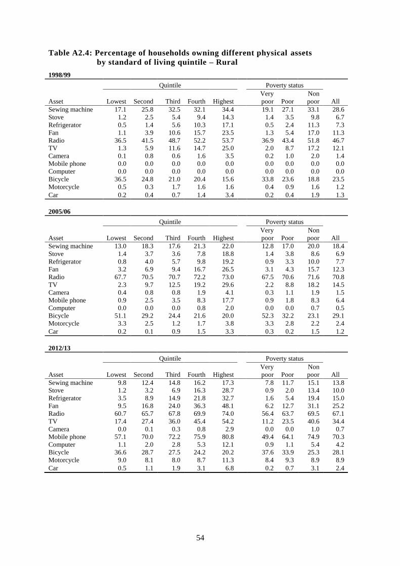
54
Table A2.4: Percentage of households owning different physical assets
by standard of living quintile – Rural
1998/99
Asset
Quintile Poverty status
All Lowest Second Third Fourth Highest
Very
poor Poor
Non
poor
Sewing machine 17.1 25.8 32.5 32.1 34.4
19.1 27.1 33.1 28.6
Stove 1.2 2.5 5.4 9.4 14.3
1.4 3.5 9.8 6.7
Refrigerator 0.5 1.4 5.6 10.3 17.1
0.5 2.4 11.3 7.3
Fan 1.1 3.9 10.6 15.7 23.5
1.3 5.4 17.0 11.3
Radio 36.5 41.5 48.7 52.2 53.7
36.9 43.4 51.8 46.7
TV 1.3 5.9 11.6 14.7 25.0
2.0 8.7 17.2 12.1
Camera 0.1 0.8 0.6 1.6 3.5
0.2 1.0 2.0 1.4
Mobile phone 0.0 0.0 0.0 0.0 0.0
0.0 0.0 0.0 0.0
Computer 0.0 0.0 0.0 0.0 0.0
0.0 0.0 0.0 0.0
Bicycle 36.5 24.8 21.0 20.4 15.6
33.8 23.6 18.8 23.5
Motorcycle 0.5 0.3 1.7 1.6 1.6
0.4 0.9 1.6 1.2
Car 0.2 0.4 0.7 1.4 3.4 0.2 0.4 1.9 1.3
2005/06
Asset
Quintile Poverty status
All Lowest Second Third Fourth Highest
Very
poor Poor
Non
poor
Sewing machine 13.0 18.3 17.6 21.3 22.0
12.8 17.0 20.0 18.4
Stove 1.4 3.7 3.6 7.8 18.8
1.4 3.8 8.6 6.9
Refrigerator 0.8 4.0 5.7 9.8 19.2
0.9 3.3 10.0 7.7
Fan 3.2 6.9 9.4 16.7 26.5
3.1 4.3 15.7 12.3
Radio 67.7 70.5 70.7 72.2 73.0
67.5 70.6 71.6 70.8
TV 2.3 9.7 12.5 19.2 29.6
2.2 8.8 18.2 14.5
Camera 0.4 0.8 0.8 1.9 4.1
0.3 1.1 1.9 1.5
Mobile phone 0.9 2.5 3.5 8.3 17.7
0.9 1.8 8.3 6.4
Computer 0.0 0.0 0.0 0.8 2.0
0.0 0.0 0.7 0.5
Bicycle 51.1 29.2 24.4 21.6 20.0
52.3 32.2 23.1 29.1
Motorcycle 3.3 2.5 1.2 1.7 3.8
3.3 2.8 2.2 2.4
Car 0.2 0.1 0.9 1.5 3.3 0.3 0.2 1.5 1.2
2012/13
Asset
Quintile Poverty status
All Lowest Second Third Fourth Highest
Very
poor Poor
Non
poor
Sewing machine 9.8 12.4 14.8 16.2 17.3
7.8 11.7 15.1 13.8
Stove 1.2 3.2 6.9 16.3 28.7
0.9 2.0 13.4 10.0
Refrigerator 3.5 8.9 14.9 21.8 32.7
1.6 5.4 19.4 15.0
Fan 9.5 16.8 24.0 36.3 48.1
6.2 12.7 31.1 25.2
Radio 60.7 65.7 67.8 69.9 74.0
56.4 63.7 69.5 67.1
TV 17.4 27.4 36.0 45.4 54.2
11.2 23.5 40.6 34.4
Camera 0.0 0.1 0.3 0.8 2.9
0.0 0.0 1.0 0.7
Mobile phone 57.1 70.0 72.2 75.9 80.8
49.4 64.1 74.9 70.3
Computer 1.1 2.0 2.8 5.3 12.1
0.9 1.1 5.4 4.2
Bicycle 36.6 28.7 27.5 24.2 20.2
37.6 33.9 25.3 28.1
Motorcycle 9.0 8.1 8.0 8.7 11.3
8.4 9.3 8.9 8.9
Car 0.5 1.1 1.9 3.1 6.8 0.2 0.7 3.1 2.4
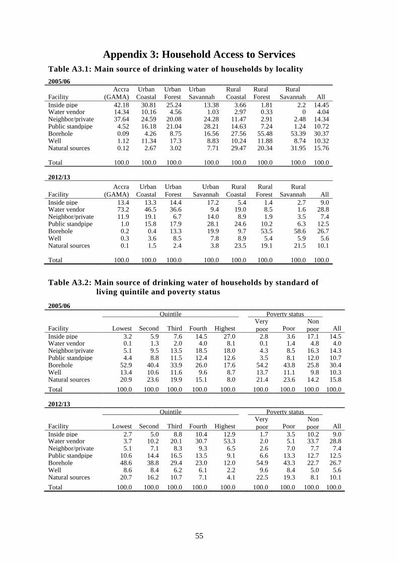
55
Appendix 3: Household Access to Services
Table A3.1: Main source of drinking water of households by locality
2005/06
Facility
Accra
(GAMA)
Urban
Coastal
Urban
Forest
Urban
Savannah
Rural
Coastal
Rural
Forest
Rural
Savannah All
Inside pipe 42.18 30.81 25.24 13.38 3.66 1.81 2.2 14.45 Water vendor 14.34 10.16 4.56 1.03 2.97 0.33 0 4.04 Neighbor/private 37.64 24.59 20.08 24.28 11.47 2.91 2.48 14.34 Public standpipe 4.52 16.18 21.04 28.21 14.63 7.24 1.24 10.72 Borehole 0.09 4.26 8.75 16.56 27.56 55.48 53.39 30.37 Well 1.12 11.34 17.3 8.83 10.24 11.88 8.74 10.32 Natural sources 0.12 2.67 3.02 7.71 29.47 20.34 31.95 15.76
Total 100.0 100.0 100.0 100.0 100.0 100.0 100.0 100.0
2012/13
Facility
Accra
(GAMA)
Urban
Coastal
Urban
Forest
Urban
Savannah
Rural
Coastal
Rural
Forest
Rural
Savannah All
Inside pipe 13.4 13.3 14.4 17.2 5.4 1.4 2.7 9.0 Water vendor 73.2 46.5 36.6 9.4 19.0 8.5 1.6 28.8 Neighbor/private 11.9 19.1 6.7 14.0 8.9 1.9 3.5 7.4 Public standpipe 1.0 15.8 17.9 28.1 24.6 10.2 6.3 12.5 Borehole 0.2 0.4 13.3 19.9 9.7 53.5 58.6 26.7 Well 0.3 3.6 8.5 7.8 8.9 5.4 5.9 5.6 Natural sources 0.1 1.5 2.4 3.8 23.5 19.1 21.5 10.1
Total 100.0 100.0 100.0 100.0 100.0 100.0 100.0 100.0
Table A3.2: Main source of drinking water of households by standard of
living quintile and poverty status
2005/06
Facility
Quintile Poverty status
Lowest Second Third Fourth Highest Very
poor Poor Non
poor All
Inside pipe 3.2 5.9 7.6 14.5 27.0
2.8 3.6 17.1 14.5 Water vendor 0.1 1.3 2.0 4.0 8.1
0.1 1.4 4.8 4.0
Neighbor/private 5.1 9.5 13.5 18.5 18.0
4.3 8.5 16.3 14.3 Public standpipe 4.4 8.8 11.5 12.4 12.6
3.5 8.1 12.0 10.7
Borehole 52.9 40.4 33.9 26.0 17.6
54.2 43.8 25.8 30.4 Well 13.4 10.6 11.6 9.6 8.7
13.7 11.1 9.8 10.3
Natural sources 20.9 23.6 19.9 15.1 8.0
21.4 23.6 14.2 15.8
Total 100.0 100.0 100.0 100.0 100.0 100.0 100.0 100.0 100.0
2012/13
Facility
Quintile Poverty status
Lowest Second Third Fourth Highest Very
poor Poor Non
poor All
Inside pipe 2.7 5.0 8.8 10.4 12.9
1.7 3.5 10.2 9.0 Water vendor 3.7 10.2 20.1 30.7 53.3
2.0 5.1 33.7 28.8
Neighbor/private 5.1 7.1 8.3 9.3 6.5
2.6 7.0 7.7 7.4 Public standpipe 10.6 14.4 16.5 13.5 9.1
6.6 13.3 12.7 12.5
Borehole 48.6 38.8 29.4 23.0 12.0
54.9 43.3 22.7 26.7 Well 8.6 8.4 6.2 6.1 2.2
9.6 8.4 5.0 5.6
Natural sources 20.7 16.2 10.7 7.1 4.1
22.5 19.3 8.1 10.1
Total 100.0 100.0 100.0 100.0 100.0 100.0 100.0 100.0 100.0
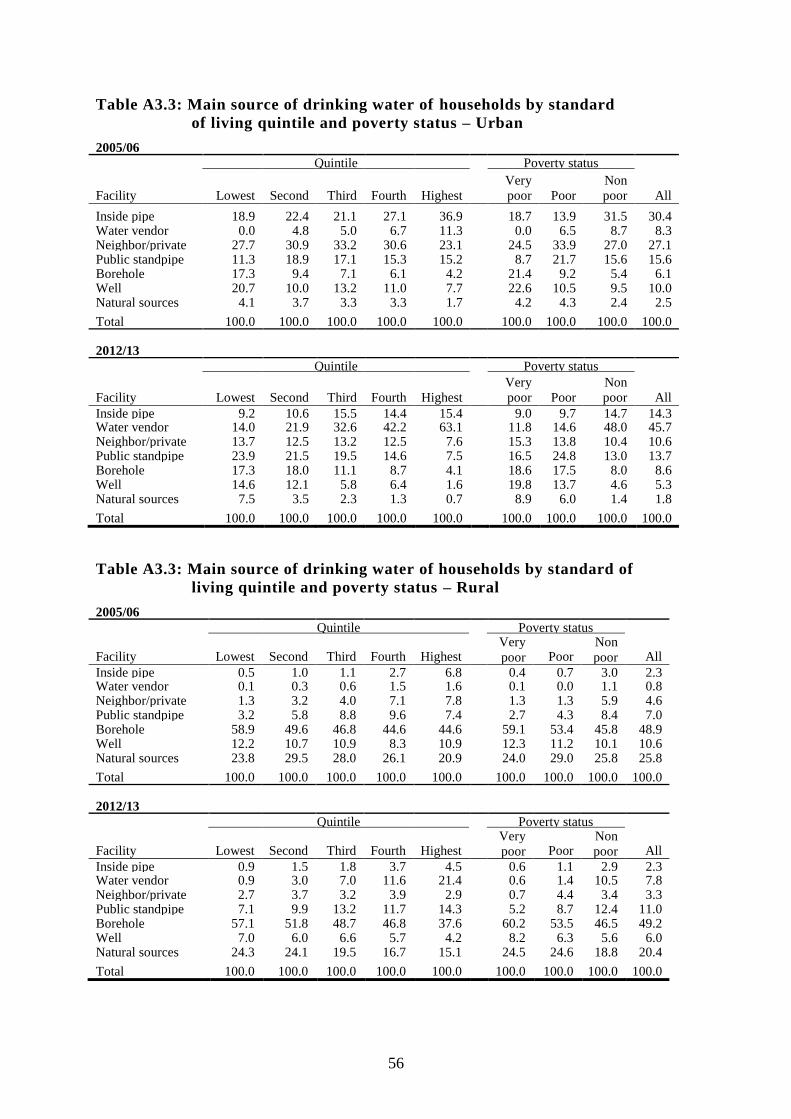
56
Table A3.3: Main source of drinking water of households by standard
of living quintile and poverty status – Urban
2005/06
Facility
Quintile Poverty status
Lowest Second Third Fourth Highest
Very
poor Poor
Non
poor All
Inside pipe 18.9 22.4 21.1 27.1 36.9
18.7 13.9 31.5 30.4 Water vendor 0.0 4.8 5.0 6.7 11.3
0.0 6.5 8.7 8.3
Neighbor/private 27.7 30.9 33.2 30.6 23.1
24.5 33.9 27.0 27.1 Public standpipe 11.3 18.9 17.1 15.3 15.2
8.7 21.7 15.6 15.6
Borehole 17.3 9.4 7.1 6.1 4.2
21.4 9.2 5.4 6.1 Well 20.7 10.0 13.2 11.0 7.7
22.6 10.5 9.5 10.0
Natural sources 4.1 3.7 3.3 3.3 1.7
4.2 4.3 2.4 2.5
Total 100.0 100.0 100.0 100.0 100.0 100.0 100.0 100.0 100.0
2012/13
Facility
Quintile Poverty status
Lowest Second Third Fourth Highest
Very
poor Poor
Non
poor All
Inside pipe 9.2 10.6 15.5 14.4 15.4
9.0 9.7 14.7 14.3 Water vendor 14.0 21.9 32.6 42.2 63.1
11.8 14.6 48.0 45.7
Neighbor/private 13.7 12.5 13.2 12.5 7.6
15.3 13.8 10.4 10.6 Public standpipe 23.9 21.5 19.5 14.6 7.5
16.5 24.8 13.0 13.7
Borehole 17.3 18.0 11.1 8.7 4.1
18.6 17.5 8.0 8.6 Well 14.6 12.1 5.8 6.4 1.6
19.8 13.7 4.6 5.3
Natural sources 7.5 3.5 2.3 1.3 0.7
8.9 6.0 1.4 1.8
Total 100.0 100.0 100.0 100.0 100.0 100.0 100.0 100.0 100.0
Table A3.3: Main source of drinking water of households by standard of
living quintile and poverty status – Rural
2005/06
Facility
Quintile Poverty status
Lowest Second Third Fourth Highest Very
poor Poor Non
poor All
Inside pipe 0.5 1.0 1.1 2.7 6.8
0.4 0.7 3.0 2.3 Water vendor 0.1 0.3 0.6 1.5 1.6
0.1 0.0 1.1 0.8
Neighbor/private 1.3 3.2 4.0 7.1 7.8
1.3 1.3 5.9 4.6 Public standpipe 3.2 5.8 8.8 9.6 7.4
2.7 4.3 8.4 7.0
Borehole 58.9 49.6 46.8 44.6 44.6
59.1 53.4 45.8 48.9 Well 12.2 10.7 10.9 8.3 10.9
12.3 11.2 10.1 10.6
Natural sources 23.8 29.5 28.0 26.1 20.9
24.0 29.0 25.8 25.8
Total 100.0 100.0 100.0 100.0 100.0 100.0 100.0 100.0 100.0
2012/13
Facility
Quintile Poverty status
Lowest Second Third Fourth Highest Very
poor Poor Non
poor All
Inside pipe 0.9 1.5 1.8 3.7 4.5
0.6 1.1 2.9 2.3 Water vendor 0.9 3.0 7.0 11.6 21.4
0.6 1.4 10.5 7.8
Neighbor/private 2.7 3.7 3.2 3.9 2.9
0.7 4.4 3.4 3.3 Public standpipe 7.1 9.9 13.2 11.7 14.3
5.2 8.7 12.4 11.0
Borehole 57.1 51.8 48.7 46.8 37.6
60.2 53.5 46.5 49.2 Well 7.0 6.0 6.6 5.7 4.2
8.2 6.3 5.6 6.0
Natural sources 24.3 24.1 19.5 16.7 15.1
24.5 24.6 18.8 20.4
Total 100.0 100.0 100.0 100.0 100.0 100.0 100.0 100.0 100.0

57
Table A3.5: Toilet facility used by households by locality
2005/06
Facility type
Accra
(GAMA)
Urban
Coastal
Urban
Forest
Urban
Savannah
Rural
Coastal
Rural
Forest
Rural
Savannah All
Flush 33.2 22.9 17.5 5.1 1.4 1.1 0.7 10.2 Pit latrine 5.0 22.6 23.2 11.6 43.6 57.6 20.9 31.5 Pan/bucket 3.2 1.5 3.2 0.3 0.1 0.3 0.3 1.3 KVIP 15.8 9.3 15.5 14.3 11.4 11.8 4.6 11.7 Public 41.6 33.0 37.5 51.2 15.8 21.7 4.6 25.8 Other* 1.2 10.7 3.1 17.4 27.7 7.5 68.9 19.6
Total 100.0 100.0 100.0 100.0 100.0 100.0 100.0 100.0
2012/13
Facility type
Accra
(GAMA)
Urban
Coastal
Urban
Forest
Urban
Savannah
Rural
Coastal
Rural
Forest
Rural
Savannah All
Flush 34.2 21.2 21.1 5.7 5.0 2.5 0.8 13.9 Pit latrine 10.0 14.2 19.7 11.8 22.2 32.6 8.7 19.1 Pan/bucket 0.5 0.4 0.2 0.2 0.0 0.2 0.0 0.2 KVIP 20.6 13.6 14.1 7.3 7.4 10.7 3.6 12.1 Public 31.3 35.2 41.9 47.9 34.2 40.7 14.3 35.7 Other* 3.5 15.5 3.0 27.1 31.2 13.4 72.7 19.1
Total 100.0 100.0 100.0 100.0 100.0 100.0 100.0 100.0
*Other include bush, beaches etc.
Table A3.6: Toilet facility used by households by standard of living
quintile and poverty status 2005/06
Facility
type
Quintile Poverty status
Lowest Second Third Fourth Highest
Very
poor Poor
Non
poor All
Flush 0.5 2.4 4.1 8.1 22.7
0.5 1.1 12.4 10.2 Pit latrine 26.2 39.3 37.7 34.3 24.3
25.6 38.0 31.7 31.5
Pan/bucket 0.0 0.9 0.8 1.5 2.1
0.0 0.8 1.5 1.3 KVIP 5.0 7.7 11.7 13.2 15.1
4.9 5.6 13.2 11.7
Public 13.4 23.5 26.9 30.2 28.3
11.9 23.6 28.0 25.8 Other* 55.0 26.2 18.7 12.8 7.5
57.1 31.0 13.3 19.6
Total 100.0 100.0 100.0 100.0 100.0 100.0 100.0 100.0 100.0
2012/13
Facility
type
Quintile Poverty status
Lowest Second Third Fourth Highest
Very
poor Poor
Non
poor All
Flush 1.7 3.6 6.6 13.7 29.1
0.8 2.0 16.3 13.9 Pit latrine 20.0 22.6 22.4 19.2 14.8
18.5 21.0 18.9 19.1
Pan/bucket 0.0 0.2 0.1 0.1 0.5
0.0 0.0 0.2 0.2 KVIP 3.9 8.1 11.3 16.8 14.8
2.0 5.8 13.6 12.1
Public 28.5 38.0 39.5 37.5 33.9
23.2 33.3 36.8 35.7 Other* 45.8 27.5 20.2 12.8 7.0
55.5 37.9 14.2 19.1
Total 100.0 100.0 100.0 100.0 100.0 100.0 100.0 100.0 100.0
*Other include bush, beaches etc.
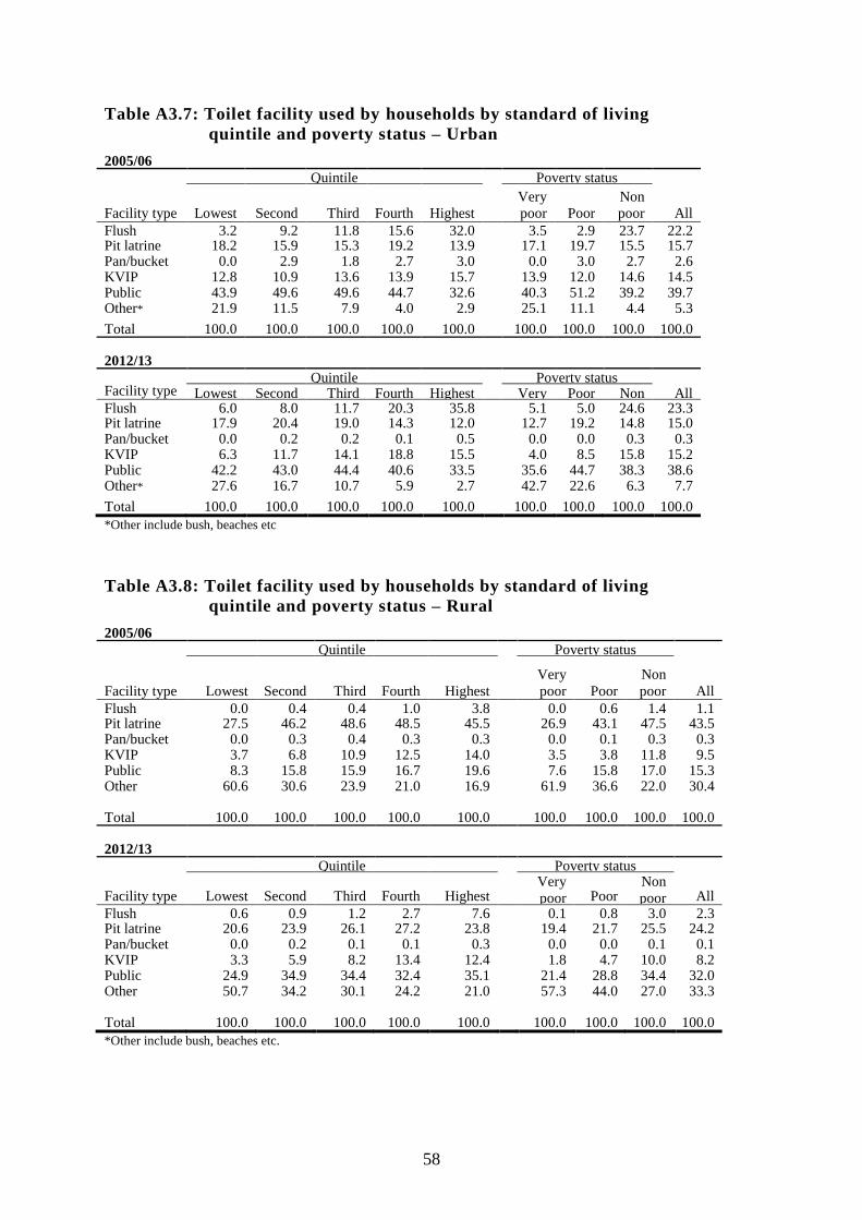
58
Table A3.7: Toilet facility used by households by standard of living
quintile and poverty status – Urban
2005/06
Facility type
Quintile Poverty status
Lowest Second Third Fourth Highest
Very
poor Poor
Non
poor All
Flush 3.2 9.2 11.8 15.6 32.0
3.5 2.9 23.7 22.2 Pit latrine 18.2 15.9 15.3 19.2 13.9
17.1 19.7 15.5 15.7
Pan/bucket 0.0 2.9 1.8 2.7 3.0
0.0 3.0 2.7 2.6 KVIP 12.8 10.9 13.6 13.9 15.7
13.9 12.0 14.6 14.5
Public 43.9 49.6 49.6 44.7 32.6
40.3 51.2 39.2 39.7 Other* 21.9 11.5 7.9 4.0 2.9
25.1 11.1 4.4 5.3
Total 100.0 100.0 100.0 100.0 100.0 100.0 100.0 100.0 100.0
2012/13
Facility type Quintile Poverty status
Lowest Second Third Fourth Highest Very
poor
Poor Non
poor
All Flush 6.0 8.0 11.7 20.3 35.8
5.1 5.0 24.6 23.3
Pit latrine 17.9 20.4 19.0 14.3 12.0
12.7 19.2 14.8 15.0 Pan/bucket 0.0 0.2 0.2 0.1 0.5
0.0 0.0 0.3 0.3
KVIP 6.3 11.7 14.1 18.8 15.5
4.0 8.5 15.8 15.2 Public 42.2 43.0 44.4 40.6 33.5
35.6 44.7 38.3 38.6
Other* 27.6 16.7 10.7 5.9 2.7
42.7 22.6 6.3 7.7
Total 100.0 100.0 100.0 100.0 100.0 100.0 100.0 100.0 100.0
*Other include bush, beaches etc
Table A3.8: Toilet facility used by households by standard of living
quintile and poverty status – Rural
2005/06
Facility type
Quintile Poverty status
Lowest Second Third Fourth Highest
Very
poor Poor
Non
poor All
Flush 0.0 0.4 0.4 1.0 3.8
0.0 0.6 1.4 1.1 Pit latrine 27.5 46.2 48.6 48.5 45.5
26.9 43.1 47.5 43.5
Pan/bucket 0.0 0.3 0.4 0.3 0.3
0.0 0.1 0.3 0.3 KVIP 3.7 6.8 10.9 12.5 14.0
3.5 3.8 11.8 9.5
Public 8.3 15.8 15.9 16.7 19.6
7.6 15.8 17.0 15.3 Other 60.6 30.6 23.9 21.0 16.9
61.9 36.6 22.0 30.4
Total 100.0 100.0 100.0 100.0 100.0 100.0 100.0 100.0 100.0
2012/13
Facility type
Quintile Poverty status
Lowest Second Third Fourth Highest Very
poor Poor Non
poor All
Flush 0.6 0.9 1.2 2.7 7.6
0.1 0.8 3.0 2.3 Pit latrine 20.6 23.9 26.1 27.2 23.8
19.4 21.7 25.5 24.2
Pan/bucket 0.0 0.2 0.1 0.1 0.3
0.0 0.0 0.1 0.1 KVIP 3.3 5.9 8.2 13.4 12.4
1.8 4.7 10.0 8.2
Public 24.9 34.9 34.4 32.4 35.1
21.4 28.8 34.4 32.0 Other 50.7 34.2 30.1 24.2 21.0
57.3 44.0 27.0 33.3
Total 100.0 100.0 100.0 100.0 100.0 100.0 100.0 100.0 100.0
*Other include bush, beaches etc.
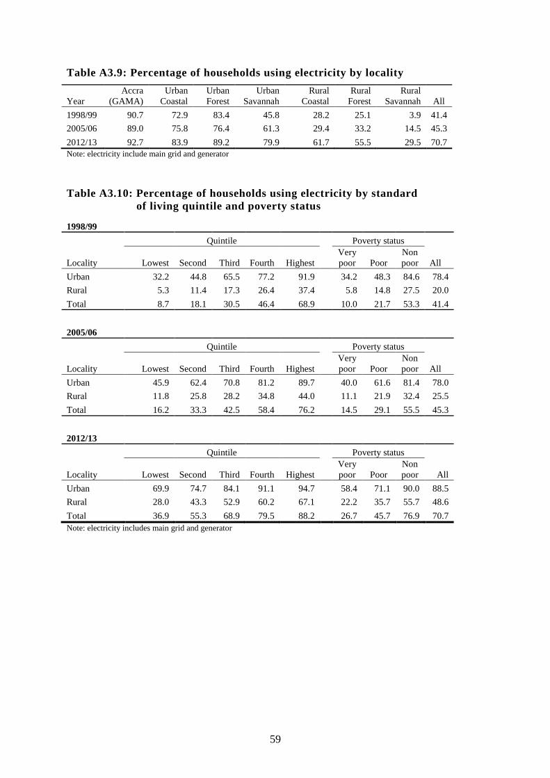
59
Table A3.9: Percentage of households using electricity by locality
Year
Accra
(GAMA)
Urban
Coastal
Urban
Forest
Urban
Savannah
Rural
Coastal
Rural
Forest
Rural
Savannah All
1998/99 90.7 72.9 83.4 45.8 28.2 25.1 3.9 41.4
2005/06 89.0 75.8 76.4 61.3 29.4 33.2 14.5 45.3
2012/13 92.7 83.9 89.2 79.9 61.7 55.5 29.5 70.7
Note: electricity include main grid and generator
Table A3.10: Percentage of households using electricity by standard
of living quintile and poverty status
1998/99
Locality
Quintile Poverty status
Lowest Second Third Fourth Highest
Very
poor Poor
Non
poor All
Urban 32.2 44.8 65.5 77.2 91.9
34.2 48.3 84.6 78.4
Rural 5.3 11.4 17.3 26.4 37.4
5.8 14.8 27.5 20.0
Total 8.7 18.1 30.5 46.4 68.9 10.0 21.7 53.3 41.4
2005/06
Locality
Quintile Poverty status
Lowest Second Third Fourth Highest
Very
poor Poor
Non
poor All
Urban 45.9 62.4 70.8 81.2 89.7
40.0 61.6 81.4 78.0
Rural 11.8 25.8 28.2 34.8 44.0
11.1 21.9 32.4 25.5
Total 16.2 33.3 42.5 58.4 76.2 14.5 29.1 55.5 45.3
2012/13
Locality
Quintile Poverty status
Lowest Second Third Fourth Highest
Very
poor Poor
Non
poor All
Urban 69.9 74.7 84.1 91.1 94.7
58.4 71.1 90.0 88.5
Rural 28.0 43.3 52.9 60.2 67.1
22.2 35.7 55.7 48.6
Total 36.9 55.3 68.9 79.5 88.2 26.7 45.7 76.9 70.7
Note: electricity includes main grid and generator
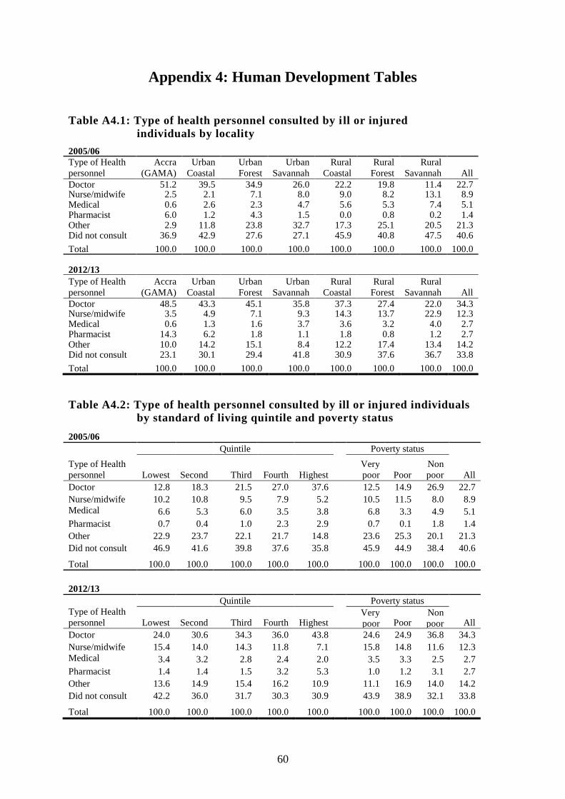
60
Appendix 4: Human Development Tables
Table A4.1: Type of health personnel consulted by i ll or injured
individuals by locality
2005/06
Type of Health
personnel
Accra
(GAMA)
Urban
Coastal
Urban
Forest
Urban
Savannah
Rural
Coastal
Rural
Forest
Rural
Savannah All
Doctor 51.2 39.5 34.9 26.0 22.2 19.8 11.4 22.7 Nurse/midwife 2.5 2.1 7.1 8.0 9.0 8.2 13.1 8.9 Medical
Assistant
0.6 2.6 2.3 4.7 5.6 5.3 7.4 5.1 Pharmacist 6.0 1.2 4.3 1.5 0.0 0.8 0.2 1.4 Other 2.9 11.8 23.8 32.7 17.3 25.1 20.5 21.3 Did not consult 36.9 42.9 27.6 27.1 45.9 40.8 47.5 40.6
Total 100.0 100.0 100.0 100.0 100.0 100.0 100.0 100.0
2012/13 Type of Health
personnel
Accra
(GAMA)
Urban
Coastal
Urban
Forest
Urban
Savannah
Rural
Coastal
Rural
Forest
Rural
Savannah All
Doctor 48.5 43.3 45.1 35.8 37.3 27.4 22.0 34.3 Nurse/midwife 3.5 4.9 7.1 9.3 14.3 13.7 22.9 12.3 Medical
Assistant
0.6 1.3 1.6 3.7 3.6 3.2 4.0 2.7 Pharmacist 14.3 6.2 1.8 1.1 1.8 0.8 1.2 2.7 Other 10.0 14.2 15.1 8.4 12.2 17.4 13.4 14.2 Did not consult 23.1 30.1 29.4 41.8 30.9 37.6 36.7 33.8
Total 100.0 100.0 100.0 100.0 100.0 100.0 100.0 100.0
Table A4.2: Type of health personnel consulted by ill or injured individuals
by standard of living quintile and poverty status
2005/06
Type of Health
personnel
Quintile Poverty status
Lowest Second Third Fourth Highest
Very
poor Poor
Non
poor All
Doctor 12.8 18.3 21.5 27.0 37.6
12.5 14.9 26.9 22.7
Nurse/midwife 10.2 10.8 9.5 7.9 5.2
10.5 11.5 8.0 8.9
Medical
Assistant 6.6 5.3 6.0 3.5 3.8
6.8 3.3 4.9 5.1
Pharmacist 0.7 0.4 1.0 2.3 2.9
0.7 0.1 1.8 1.4
Other 22.9 23.7 22.1 21.7 14.8
23.6 25.3 20.1 21.3
Did not consult 46.9 41.6 39.8 37.6 35.8
45.9 44.9 38.4 40.6
Total 100.0 100.0 100.0 100.0 100.0 100.0 100.0 100.0 100.0
2012/13
Type of Health
personnel
Quintile Poverty status
Lowest Second Third Fourth Highest Very
poor Poor Non
poor All
Doctor 24.0 30.6 34.3 36.0 43.8
24.6 24.9 36.8 34.3
Nurse/midwife 15.4 14.0 14.3 11.8 7.1
15.8 14.8 11.6 12.3
Medical
Assistant 3.4 3.2 2.8 2.4 2.0
3.5 3.3 2.5 2.7
Pharmacist 1.4 1.4 1.5 3.2 5.3
1.0 1.2 3.1 2.7
Other 13.6 14.9 15.4 16.2 10.9
11.1 16.9 14.0 14.2
Did not consult 42.2 36.0 31.7 30.3 30.9
43.9 38.9 32.1 33.8
Total 100.0 100.0 100.0 100.0 100.0 100.0 100.0 100.0 100.0

61
Table A4.3: Type of health personnel consulted by ill or injured individuals
by standard of living quintile and poverty status - Urban
2005/06
Type of Health
personnel
Quintile Poverty status
Lowest Second Third Fourth Highest
Very
poor Poor
Non
poor All
Doctor 22.0 36.0 36.8 34.7 42.9
18.8 28.2 38.8 37.2
Nurse/midwife 9.2 8.3 3.6 6.3 4.4
9.9 6.3 5.2 5.5
Medical Assistant 4.5 0.1 1.4 3.2 2.7
4.8 0.9 2.4 2.5
Pharmacist 1.7 2.9 3.5 4.3 3.5
1.3 0.9 3.8 3.6
Other 37.8 20.9 26.2 20.2 11.2
39.3 24.6 17.9 19.4
Did not consult 24.8 31.8 28.7 31.3 35.3
25.9 39.1 31.9 31.9
Total 100.0 100.0 100.0 100.0 100.0 100.0 100.0 100.0 100.0
2012/13
Type of Health
personnel
Quintile Poverty status
Lowest Second Third Fourth Highest
Very
poor Poor
Non
poor All
Doctor 35.7 37.7 44.9 41.4 49.4
41.5 33.1 44.7 43.9
Nurse/midwife 7.6 4.2 9.8 7.5 4.6
4.7 8.1 6.4 6.5
Medical Assistant 1.9 2.2 2.2 1.7 1.2
1.5 2.0 1.7 1.7
Pharmacist 5.8 3.1 3.0 4.8 6.2
5.7 4.0 4.7 4.7
Other 10.6 13.6 12.1 17.9 9.1
7.4 14.4 12.7 12.7
Did not consult 38.4 39.2 28.0 26.7 29.6
39.3 38.6 29.7 30.4
Total 100.0 100.0 100.0 100.0 100.0 100.0 100.0 100.0 100.0
Table A4.4: Type of health personnel consulted by ill or injured individuals
by standard of living quintile and poverty status - Rural
2005/06
Type of Health
personnel
Quintile Poverty status
Lowest Second Third Fourth Highest
Very
poor Poor
Non
poor All
Doctor 11.8 15.5 16.1 20.9 27.9 11.9 13.3 19.3 16.6 Nurse/midwife 10.3 11.2 11.6 9.2 6.7
10.6 12.1 9.8 10.3 Medical
Assistant
6.8 6.1 7.7 3.8 5.9
7.0 3.6 6.5 6.2 Pharmacist 0.6 0.1 0.2 0.7 1.6
0.6 0.0 0.5 0.5
Other 21.3 24.1 20.7 22.8 21.4
22.1 25.3 21.5 22.2 Did not consult 49.3 43.1 43.8 42.6 36.5
47.9 45.6 42.5 44.3
Total 100.0 100.0 100.0 100.0 100.0 100.0 100.0 100.0 100.0
2012/13
Type of Health
personnel
Quintile Poverty status
Lowest Second Third Fourth Highest
Very
poor Poor
Non
poor All
Doctor 21.6 27.1 26.0 29.6 31.8
22.1 22.8 28.3 26.5 Nurse/midwife 17.0 18.6 17.8 16.9 12.6
17.4 16.5 17.0 17.0
Medical
Assistant
3.7 3.7 3.2 3.3 3.5
3.8 3.6 3.4 3.5 Pharmacist 0.5 0.7 0.4 1.3 3.3
0.4 0.5 1.3 1.0
Other 14.3 15.5 18.0 14.2 15.0
11.7 17.6 15.4 15.4 Did not consult 42.9 34.4 34.7 34.7 33.8
44.6 39.0 34.6 36.6
Total 100.0 100.0 100.0 100.0 100.0 100.0 100.0 100.0 100.0
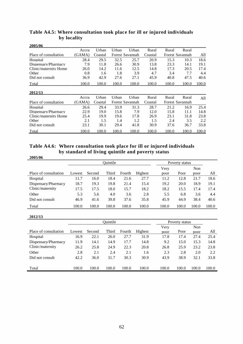
62
Table A4.5: Where consultation took place for ill or injured individuals
by locality
2005/06
Place of consultation
Accra
(GAMA)
Urban
Coastal
Urban
Forest
Urban
Savannah
Rural
Coastal
Rural
Forest
Rural
Savannah All
Hospital 28.4 29.5 32.5 25.7 20.9 15.3 10.3 18.6 Dispensary/Pharmacy 7.9 11.8 26.6 30.9 13.8 23.3 14.1 19.1 Clinic/maternity Home 26.0 14.2 11.6 12.5 14.8 17.3 20.5 17.4 Other 0.8 1.6 1.8 3.9 4.7 3.4 7.7 4.4 Did not consult 36.9 42.9 27.6 27.1 45.9 40.8 47.5 40.6
Total 100.0 100.0 100.0 100.0 100.0 100.0 100.0 100.0
2012/13
Place of consultation
Accra
(GAMA)
Urban
Coastal
Urban
Forest
Urban
Savannah
Rural
Coastal
Rural
Forest
Rural
Savannah All
Hospital 26.6 29.4 33.9 31.3 28.7 21.2 16.9 25.4 Dispensary/Pharmacy 22.9 19.0 15.8 7.9 12.0 15.8 11.1 14.8 Clinic/maternity Home 25.4 19.9 19.6 17.8 26.9 23.1 31.8 23.8 Other 2.1 1.5 1.4 1.2 1.5 2.4 3.5 2.2 Did not consult 23.1 30.1 29.4 41.8 30.9 37.6 36.7 33.8
Total 100.0 100.0 100.0 100.0 100.0 100.0 100.0 100.0
Table A4.6: Where consultation took place for ill or injured individuals
by standard of living quintile and poverty status
2005/06
Place of consultation
Quintile Poverty status
Lowest Second Third Fourth Highest
Very
poor Poor
Non
poor All
Hospital 11.7 16.0 18.4 21.6 27.7
11.2 12.8 21.7 18.6
Dispensary/Pharmacy 18.7 19.3 19.8 21.4 15.4
19.2 20.0 18.9 19.1
Clinic/maternity
Home 17.5 17.5 18.0 15.7 18.2
18.2 15.5 17.4 17.4
Other 5.3 5.6 4.0 3.6 2.8
5.5 6.8 3.6 4.4
Did not consult 46.9 41.6 39.8 37.6 35.8
45.9 44.9 38.4 40.6
Total 100.0 100.0 100.0 100.0 100.0 100.0 100.0 100.0 100.0
2012/13
Place of consultation
Quintile Poverty status
Lowest Second Third Fourth Highest Very
poor Poor Non
poor All
Hospital 16.9 22.1 26.0 27.7 31.9
17.8 17.4 27.4 25.4
Dispensary/Pharmacy 11.9 14.1 14.9 17.7 14.8
9.2 15.0 15.3 14.8
Clinic/maternity
Home 26.2 25.8 24.9 22.3 20.8
26.8 25.9 23.2 23.8
Other 2.8 2.1 2.4 2.1 1.6
2.3 2.8 2.0 2.2
Did not consult 42.2 36.0 31.7 30.3 30.9
43.9 38.9 32.1 33.8
Total 100.0 100.0 100.0 100.0 100.0 100.0 100.0 100.0 100.0

63
Table A4.7: Where consultation took place for ill or injured individuals
by standard of living quintile and poverty status – Urban
2005/06
Place of consultation
Quintile Poverty status
Lowest Second Third Fourth Highest
Very
poor Poor
Non
poor All
Hospital 20.4 28.8 26.7 29.1 34.0
16.8 23.3 30.9 29.8
Dispensary/Pharmacy 32.3 22.0 28.0 23.4 13.6
32.2 23.3 20.4 21.2
Clinic/maternity
Home 16.4 15.5 14.6 14.8 15.4
17.9 12.1 15.1 15.2
Other 6.1 1.9 2.0 1.4 1.7
7.2 2.2 1.6 2.0
Did not consult 24.8 31.8 28.7 31.3 35.3
25.9 39.1 31.9 31.9
Total 100.0 100.0 100.0 100.0 100.0 100.0 100.0 100.0 100.0
2012/13
Place of consultation
Quintile Poverty status
Lowest Second Third Fourth Highest Very
poor Poor Non
poor All
Hospital 24.4 26.0 33.4 30.5 34.6
31.6 20.7 32.2 31.4
Dispensary/Pharmacy 14.2 15.1 13.9 21.3 14.3
10.6 16.2 16.2 16.1
Clinic/maternity
Home 21.3 19.0 22.9 19.8 20.1
16.1 23.6 20.4 20.5
Other 1.7 0.7 1.9 1.8 1.4
2.4 0.9 1.5 1.5
Did not consult 38.4 39.2 28.0 26.7 29.6
39.3 38.6 29.7 30.4
Total 100.0 100.0 100.0 100.0 100.0 100.0 100.0 100.0 100.0
Table A4.8: Where consultation took place for ill or injured individuals
by standard of living quintile and poverty status - Rural 2005/06
Place of consultation
Quintile Poverty status
Lowest Second Third Fourth Highest
Very
poor Poor
Non
poor All
Hospital 10.7 14.0 15.4 15.8 16.4
10.7 11.5 15.8 13.9
Dispensary/Pharmacy 17.2 18.9 16.9 19.8 18.9
17.9 19.6 17.9 18.2
Clinic/maternity
Home 17.7 17.9 19.2 16.4 23.4
18.3 15.9 18.9 18.3
Other 5.2 6.2 4.8 5.4 4.9
5.3 7.4 4.9 5.4
Did not consult 49.3 43.1 43.8 42.6 36.5
47.9 45.6 42.5 44.3
Total 100.0 100.0 100.0 100.0 100.0 100.0 100.0 100.0 100.0
2012/13
Place of consultation
Quintile Poverty status
Lowest Second Third Fourth Highest Very
poor Poor Non
poor All
Hospital 15.4 20.2 20.2 24.3 26.3
15.8 16.6 22.3 20.5
Dispensary/Pharmacy 11.4 13.7 15.8 13.4 15.8
9.0 14.7 14.2 13.8
Clinic/maternity
Home 27.2 29.0 26.5 25.3 22.2
28.4 26.5 26.3 26.5
Other 3.1 2.8 2.8 2.4 1.9
2.3 3.2 2.6 2.7
Did not consult 42.9 34.4 34.7 34.7 33.8
44.6 39.0 34.6 36.6
Total 100.0 100.0 100.0 100.0 100.0 100.0 100.0 100.0 100.0

64
Table A4.9: Net enrolment in primary school, by locality, gender and
standard of living quintile
2005/06
Locality Sex
Quintile Poverty status
Lowest Second Third Fourth Highest
Very
poor Poor
Non
poor All
Urban Male 61.8 70.9 79.3 82.2 83.9
61.3 63.2 81.5 78.4
Female 74.3 70.3 74.9 79.4 88.2
74.1 68.4 80.9 79.7
All 67.3 70.6 77.1 80.8 86.4 66.9 65.6 81.2 79.1
Rural Male 51.1 65.9 68.2 71.5 83.2
50.1 61.6 70.9 61.5
Female 48.7 61.6 67.5 66.4 70.7
48.3 60.5 66.0 58.6
All 50.0 63.8 67.9 68.9 77.4 49.2 61.1 68.6 60.1
Total Male 52.0 66.8 71.5 77.3 83.7
52.0 66.8 71.5 66.3
Female 50.8 63.3 69.8 73.4 84.4
50.8 63.3 69.8 65.4
All 51.5 65.1 70.7 75.3 84.1 51.5 65.1 70.7 65.8
Computed from GLSS 5 (2005/06)
2012/13
Locality Sex
Quintile Poverty status
Lowest Second Third Fourth Highest
Very
poor Poor
Non
poor All
Urban Male 69.5 76.6 79.4 81.8 88.3
78.7 67.4 81.8 79.6
Female 69.4 76.9 82.1 82.7 84.1
52.2 74.7 81.8 80.2
All 69.5 76.7 80.8 82.3 86.1 68.6 70.8 81.8 79.9
Rural Male 60.8 69.2 72.6 70.1 74.1
59.3 63.8 71.1 66.2
Female 60.7 68.3 73.6 73.9 77.1
58.6 64.6 71.9 66.6
All 60.7 68.8 73.1 72.1 75.7 59.0 64.2 71.5 66.4
Total Male 61.9 71.4 75.4 76.6 83.7
60.5 64.6 75.9 70.6
Female 61.7 70.9 77.5 78.9 81.9
58.3 66.5 76.7 71.2
All 61.8 71.2 76.4 77.8 82.8 59.5 65.5 76.3 70.9
Computed from GLSS 5 (2012/13)
Notes: Cells with less than 30 observations are marked with *. “Very poor” correspond to those lying below the extreme
poverty line, “poor” to those below the poverty line but above the extreme poverty line, and “non-poor” to those above the
poverty line.

65
Table A4.10: Net enrolment in JSS/JHS, by locality, sex poverty status
and standard of living quintile
2005/06
Locality Sex
Quintile Poverty status
All Lowest Second Third Fourth Highest
Very
poor Poor
Non
poor
Urban Male *23.1 *25.3 37.0 51.9 46.2
26.5 23.5 43.3
40.7
Female *10.3 *23.3 44.8 35.5 43.0
8.8 21.1 39.2
36.5
All *16.7 24.4 40.8 43.4 44.3 17.6 22.6 41.1 38.5
Rural Male 7.4 17.5 17.1 29.3 15.4
6.9 16.9 20.1
14.6
Female 8.9 20.0 22.2 22.2 21.4
9.0 13.6 22.5
16.8
All 8.0 18.7 19.6 25.9 18.5 7.8 15.3 21.3 15.6
Total Male 8.7 19.3 23.9 41.4 39.1
8.5 18.2 30.8
23.0
Female 9.0 20.7 29.7 29.7 38.9
9.0 14.6 30.7
23.9
All 8.9 20.0 26.8 35.5 39.0 8.7 16.6 30.7 23.4
Computed from GLSS 5 (2005/06)
2012/13
Locality Sex
Quintile Poverty status
All Lowest Second Third Fourth Highest
Very
poor Poor
Non
poor
Urban Male *16.8 33.5 35.4 41.4 48.7
*7.4 22.7 39.8
36.6
Female *18.3 32.0 34.2 38.6 56.7
*20.7 *19.7 41.1
37.9
All 17.6 32.8 34.8 39.8 53.1 *14.3 21.2 40.5 37.3
Rural Male 10.2 18.0 17.7 *15.0 34.8
7.1 13.8 19.6
14.6
Female 10.6 20.2 20.6 25.7 39.4
8.6 15.2 23.3
17.7
All 10.3 19.0 19.1 20.5 37.2 7.7 14.4 21.4 16.0
Total Male 10.9 22.8 25.9 29.3 44.4
7.1 15.6 29.2
21.9
Female 11.7 24.1 27.5 33.6 51.8
9.4 16.3 32.7
25.7
All 11.2 23.4 26.7 31.6 48.4 8.1 15.9 31.0 23.8
Computed from GLSS 5 (2012/13)
Notes: Cells with less than 30 observations are marked with *. “Very poor” correspond to those lying below the extreme
poverty line, “poor” to those below the poverty line but above the extreme poverty line, and “non-poor” to those above the
poverty line.
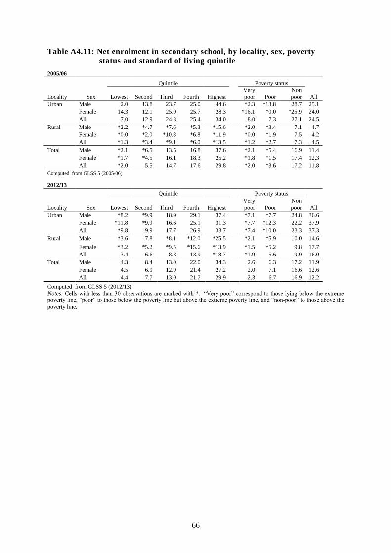
66
Table A4.11: Net enrolment in secondary school, by locality, sex, poverty
status and standard of living quintile
2005/06
Locality Sex
Quintile Poverty status
All Lowest Second Third Fourth Highest
Very
poor Poor
Non
poor
Urban Male 2.0 13.8 23.7 25.0 44.6
*2.3 *13.8 28.7 25.1
Female 14.3 12.1 25.0 25.7 28.3
*16.1 *0.0 *25.9 24.0
All 7.0 12.9 24.3 25.4 34.0 8.0 7.3 27.1 24.5
Rural Male *2.2 *4.7 *7.6 *5.3 *15.6
*2.0 *3.4 7.1 4.7
Female *0.0 *2.0 *10.8 *6.8 *11.9
*0.0 *1.9 7.5 4.2
All *1.3 *3.4 *9.1 *6.0 *13.5 *1.2 *2.7 7.3 4.5
Total Male *2.1 *6.5 13.5 16.8 37.6
*2.1 *5.4 16.9 11.4
Female *1.7 *4.5 16.1 18.3 25.2
*1.8 *1.5 17.4 12.3
All *2.0 5.5 14.7 17.6 29.8 *2.0 *3.6 17.2 11.8
Computed from GLSS 5 (2005/06)
2012/13
Locality Sex
Quintile Poverty status
All Lowest Second Third Fourth Highest
Very
poor Poor
Non
poor
Urban Male *8.2 *9.9 18.9 29.1 37.4
*7.1 *7.7 24.8 36.6
Female *11.8 *9.9 16.6 25.1 31.3
*7.7 *12.3 22.2 37.9
All *9.8 9.9 17.7 26.9 33.7 *7.4 *10.0 23.3 37.3
Rural Male *3.6 7.8 *8.1 *12.0 *25.5
*2.1 *5.9 10.0 14.6
Female *3.2 *5.2 *9.5 *15.6 *13.9
*1.5 *5.2 9.8 17.7
All 3.4 6.6 8.8 13.9 *18.7 *1.9 5.6 9.9 16.0
Total Male 4.3 8.4 13.0 22.0 34.3
2.6 6.3 17.2 11.9
Female 4.5 6.9 12.9 21.4 27.2
2.0 7.1 16.6 12.6
All 4.4 7.7 13.0 21.7 29.9 2.3 6.7 16.9 12.2
Computed from GLSS 5 (2012/13)
Notes: Cells with less than 30 observations are marked with *. “Very poor” correspond to those lying below the extreme
poverty line, “poor” to those below the poverty line but above the extreme poverty line, and “non-poor” to those above the
poverty line.

67
Appendix 5: Consumption poverty using 2005/6 poverty lines
Table A5.1: Indices of Poverty by locality using the old poverty line: GH¢370.89
2005/06
Locality
Population
share
Average
Welfare Poverty indices
Contribution to national
poverty
P0 P1 P2 P1/P0 C0 C1 C2 Accra (GAMA) 11.7 1,122.91 10.6 2.9 1.1 27.0
4.4 3.5 2.8
Urban Coastal 5.8 1,236.52 5.5 0.9 0.2 16.5
1.1 0.5 0.3 Urban Forest 14.7 1,031.60 7.0 1.8 0.7 25.8
3.6 2.8 2.4
Urban Savannah 5.4 747.90 26.9 9.3 4.4 34.7
5.1 5.3 5.2 Rural Coastal 10.9 669.70 23.9 5.3 1.8 22.2
9.2 6.0 4.2
Rural Forest 28.1 623.71 27.9 6.8 2.4 24.3
27.4 19.8 14.4 Rural Savannah 23.3 397.46 60.3 25.5 13.9 42.3
49.3 62.0 70.7
Ghana 100.0 736.80 28.5 9.6 4.6 33.6 100.0 100.0 100.0 2012/13
Population
share
Average
Welfare
Poverty indices
Contribution to national
poverty
Locality P0 P1 P2 P1/P0 C0 C1 C2 Accra (GAMA) 15.0 1,463.52 3.4 0.7 0.2 21.9
2.4 1.7 1.2
Urban Coastal 5.0 1,010.49 7.9 1.8 0.7 22.7
1.9 1.4 1.1 Urban Forest 22.1 1,085.68 7.9 1.5 0.5 19.5
8.2 5.1 3.7
Urban Savannah 7.9 759.39 22.7 5.3 1.9 23.4
8.4 6.3 4.9 Rural Coastal 5.6 804.47 25.8 7.3 2.9 28.3
6.7 6.1 5.4
Rural Forest 26.3 695.45 24.4 6.6 2.6 26.9
29.9 25.9 23.3 Rural Savannah 18.0 488.37 50.7 19.8 10.1 39.0
42.6 53.5 60.5
Ghana 100.0 886.93 21.4 6.7 3.0 31.0 100.0 100.0 100.0 Computed from GLSS6 (200125/13)
2005/06
Region
Population
share
Average
Welfare Poverty indices
Contribution to national
poverty
P0 P1 P2 P1/P0 C0 C1 C2 Western 10.1 779.52 8.1 1.6 0.6 20.3
4.5 2.9 2.2
Central 8.8 832.51 9.7 1.5 0.4 15.1
4.7 2.3 1.3 Greater Accra 13.9 1,089.11 5.8 1.3 0.4 22.1
4.5 3.2 2.2
Volta 7.5 632.23 15.3 2.9 0.8 18.8
6.3 3.8 2.3 Eastern 13.4 779.15 6.6 1.5 0.5 22.7
4.9 3.5 2.8
Ashanti 16.8 827.90 11.2 2.3 0.7 20.5
10.4 6.8 4.6 Brong Ahafo 9.2 665.71 15.0 3.5 1.3 23.5
7.6 5.7 4.5
Northern 12.0 474.69 38.9 13.5 6.1 34.7
25.9 28.6 28.5 Upper East 4.8 339.37 59.8 23.3 11.8 39.0
15.7 19.6 21.6
Upper West 3.6 235.28 79.1 37.7 21.8 47.6
15.6 23.7 30.0
Ghana 100.0 736.80 28.5 9.6 4.6 33.6 100.0 100.0 100.0
2012/13
Region
Population
share
Average
Welfare Poverty indices
Contribution to national
poverty
P0 P1 P2 P1/P0 C0 C1 C2 Western 9.2 876.20 18.0 4.7 1.9 26.3
7.7 6.5 5.8
Central 8.9 828.76 16.1 4.7 2.1 29.5
6.6 6.3 6.1 Greater Accra 16.3 1,415.68 5.1 1.4 0.5 27.0
3.9 3.4 2.8
Volta 8.7 731.80 29.4 8.2 3.2 28.0
11.9 10.7 9.2 Eastern 10.4 812.89 18.0 4.8 2.0 26.8
8.7 7.5 6.8
Ashanti 19.7 970.43 12.8 2.8 1.0 21.7
11.8 8.2 6.3 Brong Ahafo 9.9 748.99 24.3 6.0 2.3 24.6
11.2 8.9 7.6
Northern 10.0 534.40 45.9 17.2 8.5 37.4
21.4 25.8 28.5 Upper East 4.1 563.98 40.4 15.3 7.9 37.8
7.7 9.3 10.7
Upper West 2.9 421.40 67.8 30.5 16.8 45.1
9.1 13.2 16.1 Ghana 100.0 886.93 21.4 6.7 3.0 31.0 100.0 100.0 100.0
Computed from GLSS6 (2012/13)

68
Table A5.2: Indices of Poverty by locality using the old poverty line: GH¢288.47
2005/06
Locality
Population
share
Average
Welfare Poverty indices
Contribution to
national poverty P0 P1 P2 P1/P0 C0 C1 C2
Accra (GAMA) 11.7 1,122.91 5.2 1.3 0.4 24.5
3.4 2.6 2.0 Urban Coastal 5.8 1,236.52 1.9 0.2 0.0 8.5
0.6 0.2 0.1
Urban Forest 14.7 1,031.60 3.0 0.9 0.4 29.5
2.5 2.3 2.1 Urban Savannah 5.4 747.90 18.1 5.7 2.4 31.8
5.4 5.5 5.0
Rural Coastal 10.9 669.70 11.3 2.0 0.6 17.9
6.8 3.9 2.4 Rural Forest 28.1 623.71 14.6 2.7 0.8 18.8
22.6 13.6 8.8
Rural Savannah 23.3 397.46 45.6 17.5 8.9 38.4
58.7 71.9 79.6 Ghana 100.0 736.80 18.1 5.7 2.6 31.3 100.0 100.0 100.0
2012/13
Locality
Population
share
Average
Welfare Poverty indices
Contribution to
national poverty
P0 P1 P2 P1/P0 C0 C1 C2 Accra (GAMA) 15.0 1,665.39 1.0 0.1 0.0 12.3
1.5 0.7 0.4
Urban Coastal 5.0 1,149.87 2.1 0.5 0.2 24.5
1.1 1.0 0.9 Urban Forest 22.1 1,235.43 2.0 0.3 0.1 15.8
4.5 2.6 1.4
Urban Savannah 7.9 864.13 6.6 1.2 0.4 18.0
5.4 3.6 3.1 Rural Coastal 5.6 915.43 11.5 2.2 0.7 19.6
6.6 4.7 3.6
Rural Forest 26.3 791.38 9.3 2.1 0.8 22.7
25.4 21.1 18.7 Rural Savannah 18.0 555.73 29.7 9.8 4.4 32.9
55.4 66.4 71.9
Ghana 100.0 1,009.26 9.6 2.6 1.1 27.4 100.0 100.0 100.0 Computed from GLSS6 (2012/13)
2005/06
Region
Population
share
Average
Welfare Poverty indices
Contribution to
national poverty
P0 P1 P2 P1/P0 C0 C1 C2 Western 10.1 779.52 8.1 1.6 0.6 20.3
4.5 2.9 2.2
Central 8.8 832.51 9.7 1.5 0.4 15.1
4.7 2.3 1.3 Greater Accra 13.9 1,089.11 5.8 1.3 0.4 22.1
4.5 3.2 2.2
Volta 7.5 632.23 15.3 2.9 0.8 18.8
6.3 3.8 2.3 Eastern 13.4 779.15 6.6 1.5 0.5 22.7
4.9 3.5 2.8
Ashanti 16.8 827.90 11.2 2.3 0.7 20.5
10.4 6.8 4.6 Brong Ahafo 9.2 665.71 15.0 3.5 1.3 23.5
7.6 5.7 4.5
Northern 12.0 474.69 38.9 13.5 6.1 34.7
25.9 28.6 28.5 Upper East 4.8 339.37 59.8 23.3 11.8 39.0
15.7 19.6 21.6
Upper West 3.6 235.28 79.1 37.7 21.8 47.6
15.6 23.7 30.0 Ghana 100.0 736.80 18.1 5.7 2.6 31.3 100.0 100.0 100.0
2012/13
Population
share
Average
Welfare Poverty indices
Contribution to
national poverty
Region P0 P1 P2 P1/P0 C0 C1 C2 Western 9.2 997.06 6.3 1.5 0.6 23.8
6.1 5.3 4.6
Central 8.9 943.07 7.6 1.8 0.7 23.9
7.0 6.1 5.6 Greater Accra 16.3 1,610.95 2.0 0.4 0.1 18.6
3.4 2.3 1.7
Volta 8.7 832.73 12.1 2.3 0.8 19.2
10.9 7.7 6.2 Eastern 10.4 925.02 7.1 1.6 0.6 22.1
7.6 6.1 5.7
Ashanti 19.7 1,104.28 3.3 0.7 0.2 19.9
6.7 4.9 3.5 Brong Ahafo 9.9 852.30 7.8 1.8 0.6 23.0
8.0 6.7 5.6
Northern 10.0 608.11 24.9 8.1 3.6 32.5
25.8 30.6 33.0 Upper East 4.1 641.77 23.5 7.8 3.5 33.1
9.9 11.9 12.9
Upper West 2.9 479.52 48.8 17.0 8.1 34.8
14.6 18.5 21.1 Ghana 100.0 1,009.26 9.6 2.6 1.1 27.4 100.0 100.0 100.0 Computed from GLSS6 (2012/13)

69
Appendix 6: Macroeconomics Indicators
Table A6.1: Main macroeconomic statistics and indicators, 2005-2013
ANNEX 1; MAIN MACROECONOMIC STATISTICS AND INDICATORS, 2005 -2013
2005 2006 2007 2008 2009 2010 2011 2012 2013**
Population estimate (million) 21.37 21.88 22.39 22.90 23.42 24.23 24.61 25.87 26.48
Exchange rate (₵/$) 0.91 0.92 0.94 1.07 1.42 1.43 1.51 1.81 1.92
GDP current (million GH₵) 15,586.6 18,706.0 23,169.5 30,265.9 36,698.1 44,530.5 59,816.3 74,959.1 93,461.5
GDP current (million US$) 17,161.2 20,332.7 24,648.9 28,285.5 25,844.0 31,129.3 39,516.6 41,458.9 48,677.5
GDP constant 2006 (million GH₵) 17,602.4 18,706.0 19,913.9 21,591.9 22,454.5 24,251.9 27,891.4 30,342.6 32,507.3
GDP constant 2006 (million US$) 19,380.6 20,332.7 21,185.4 20,179.1 15,813.2 16,953.5 18,426.0 16,782.1 16,930.8
Per capita GDP (GH₵) 729.5 854.9 1,034.8 1,321.6 1,567.0 1,837.8 2,430.6 2,897.8 3,529.6
Per capita GDP (US$) 803.2 929.3 1,100.9 1,235.2 1,103.5 1,284.7 1,605.7 1,602.8 1,838.3
Indicators of growth
Growth in GDP at current market prices 21.7 20.0 23.9 30.6 21.3 21.3 34.3 25.3 24.7
Growth in GDP at constant 2006 prices 5.9 6.2 6.5 8.4 4.0 8.0 15.0 8.8 7.1
Change in GDP deflator 14.9 12.9 16.4 20.5 16.6 12.3 16.8 15.2 16.4
Cement Production ('000 tonnes) 2,534.9 2,898.1 3,184.7 3,418.8 3,239.3 3,603.8 4,437.9 4,650.0 4,869.0
Electricity generation ('000 MegaWatts) 6,787.9 8,429.0 6,978.1 8,333.5 8,958.9 10,057.7 9,976.3 11,081.8 12,867.3
** Revised

70
Appendix 7: GLSS Sample Design
The sixth round of the Ghana Living Standards Survey (GLSS6), like the previous rounds, was
designed to provide nationally and regionally representative indicators. It applied the same
sampling methodology, a two stage sampling procedure. In the first stage enumeration areas
(EAs) were selected based on the 2010 Population and Housing Census, with probability
proportional to size (number of households). At the second stage a fixed number of
households were selected by systematic sampling within each of the selected enumeration
areas.
Given the long period of time between any of the GLSS surveys and the nearest census, the
above procedure will generally not give a self-weighting sample (where the probability of
inclusion of each household is equal). This is because the number of households in an
enumeration area is likely to have changed between the survey and the census. The selected
enumeration areas will then not have been picked with probability proportional to their true
sizes.
If the selected enumeration areas were fully listed after their selection, however, then it is
possible either (i) to compute weights reflecting differential probabilities of selection of
households in different EAs; or (ii) to amend the above procedure to restore a self-weighting
sample. The former was used for GLSS 6.
In GLSS 6, the number of primary Sampling Units (PSUs) and households were increased from
580 and 8,700 to 1,200 and 18,000 respectively –an increase of about 107% over the GLSS 5
figures to cater for the needs of other developmental studies ongoing in Ghana. Overall, the
response rate for the survey was 93.2 percent (see main GLSS6 report for detailed information).

71
Appendix 8: Construction of the Standard
of Living Measure6
As noted in the text, the primary standard of living measure used in this study is total
household consumption, per adult equivalent, expressed in constant prices of Greater Accra
in January 2013. This forms the basis for both the analysis of consumption poverty (chapter
3 of the report) and for the definition of the quintile groups used in the analysis of other
aspects of living conditions (chapter 4 to 6 of the report). This appendix explains more fully
the construction of the standard of living measure and briefly summarizes how it is used in
defining poverty and quintile groups.
Measuring total household consumption expenditure7
For GLSS 6, the construction of the standard of living measure differs slightly from what was
used in the previous surveys in the components aggregated. In addition to the previous
estimation manual used for the previous GLSS, the Survey-based Harmonized Indicator
program manual (SHIP) developed by the World Bank was also used which presents detailed
guidelines and recommendations for compiling household survey data into a set of most
commonly available variables/indicators so that the results can be replicated from the original
household survey data with ease.
The first step in constructing the standard of living measure is to estimate total household
consumption expenditure. Table A8.1 sets out in detail how this is done, covering the
components, their composition and sources within the different GLSS 6 questionnaires. This
consumption measure covers food, housing and other non-food items, and includes
imputations for consumption from sources other than market purchases. These imputations
include consumption from the output of own production and imputed rent from owner-
occupied dwellings. An imputation is also made for user values derived from durable
consumer goods owned by the household, rather than including expenditure on the
acquisition of such goods (these are lumpy expenditures, e.g. purchasing a car, more like an
investment rather than consumption).
Total consumption expenditure is estimated for a twelve-month period based on information
collected with the questionnaire. In the case of frequent purchases (e.g. food purchases,
consumption of own produced food, frequently purchased non-food items such as soap,
tobacco) this is estimated by grossing up responses relating to a shorter recall period. GLSS
6 households received 6 visits at regular intervals of 5 days in the course of the survey (in
GLSS 3 eight visits at two-day intervals in rural areas and eleven visits at three-day intervals
in urban areas; seven visits at 5-day interval in the case of GLSS 4; and 11 visits at three-day
intervals in GLSS 5). In each case, in all but the first two visits, they were asked about their
purchases of each item since the last visit, and the answers to these “bounded recall”
questions (recall relative to a fixed reference point) was used as the basis for estimating
6 The methodology to measure the household-level standard of living used in this report is consistent with the one
established in the previous Patterns and Trends of Poverty in Ghana (GSS, 2007). Therefore this appendix is reproduced
from GSS (2007) although changes were made to reflect the addition of GLSS 6.
7 Refer to THE ESTIMATION OF COMPONENTS OF HOUSEHOLD INCOMES AND EXPENDITURES: A
Methodological Guide based on the Ghana Living Standards Survey, 1991/92, 1998/99 and 2005/06 and Survey-based
Harmonized Indicator Program Manual (SHIP).
72
annual expenditure or consumption. Similar principles were used to estimate annual
expenditure on frequently purchased non-food items and on consumption of own produced
food (valuing items at the price at which they could have been sold). In the case of
consumption of own produced food, the number of months in which an item was normally
consumed was used to annualize.
A longer recall period of twelve months, was used in GLSS 6 to collect information on less
frequently purchased consumption items (e.g. clothing and footwear). As noted above (as in
GLSS3-5), purchases of durable goods were not included in this, and some other expenditure
items deemed not to be associated with increases in welfare were also excluded such as
expenditure on hospital stays. This is also a lumpy sum, and it would not be reasonable to
regard a household as being significantly better off because it had to make a large
expenditure on an emergency operation. Medical expenses in the last 2 weeks (Section 3)
were also excluded, however medical services expenditure (section 9A) for the past 12
months were included in the consumption measure.
In the case of owner occupied dwellings, imputed rents were estimated based on a hedonic
equation, which related rents of rented housing to characteristics, and used this to estimate
rental values for owner-occupied dwellings based on their characteristics and amenities.
Consumption flows (user values) for durable goods were estimated based on an average
depreciation rate of 20 percent.
In GLSS 6, the value of wage payments received in kind, and consumption of the output of
non-farm enterprises owned and operated by the household were excluded, hence the minor
difference in the estimation of total household consumption from the previous surveys (SHIP
included these components as income). The sum of all the items in Table A8.1 gives the
estimate of total household consumption expenditure, which is expressed in nominal values
(current prices).
Allowing for cost of living variations
Having estimated total nominal household consumption expenditure, further steps are needed
before it is possible to compare standards of living across households. Because the standard
of living is expressed in nominal terms, it must be adjusted to allow for variations in prices
faced by households. Two sources of variations are relevant for purposes of this study:
(i) differences in the cost of living between different localities and regions at a point in
time;
(ii) variations in prices within the time periods covered by the surveys, which can occur
due to inflation and seasonality
A cost of living index was constructed capturing these different dimensions of variation.
Geographic and time differences in the cost of living were indexed to January 2013 Greater
Accra prices between food and non-food based on the monthly regional food and non-food
CPI. The differences in the share of food and non-food components of the consumption
basket were considered among regions and between rural and urban areas. These procedures
give the geographic cost of living indices reported in Table 2.1 (in the main text).
Allowing for differences in the size and composition of households
The last adjustment needed to construct a standard of living measure is to allow for
differences in the size and or composition of households. Though a simple way of doing this
would be to divide by the nominal size of the household to give total household consumption

73
expenditure per capita, this does not allow for the fact that different members (e.g. young
children and adults) have different calorie needs. A way of allowing for these differences in
calorie intake needs is, instead, to measure household size in equivalent adults, where this is
measured using an appropriate adult equivalence scale based on calorie needs of different
members (e.g. based on age, sex).
The issue in doing this in practice is which equivalence scale to use. Given that there is
currently no Ghana specific scale to use, the scale used here is based on calorie requirements
commonly used in nutritional studies in Ghana (see Table A8.2). Calorie requirements are
distinguished by age category and sex.
The standard of living measure is then calculated by dividing the estimate of total household
consumption expenditure in January 2013 Accra prices by household size measured in
number of equivalent adults. The poverty analysis is based on the distribution of this
standard of living measure over all households in the sample, weighting each household by
its size in number of persons. This household size weight means that for example a poor
household of six members is given twice the weight of an equally poor household of three
persons. Each individual (rather than each household) in the sample is given equal weight.
The standard of living measure is used both in the analysis of consumption poverty (chapter
3) and in defining quintile groups for the analysis of other aspects of living standards (chapter
4 to 6). Box 1 provides the rationale for the poverty lines used in this study. Individuals are
then defined as poor if their standard of living measure falls below the poverty line, and as
extreme poor if it falls below the lower poverty line.
Characteristics of poverty are summarized in the tables by poverty indices and the
interpretation of which is discussed in Appendix 9. The quintile groups used in chapter 4 to 6
are based on the quintile points of the (weighted) distribution over individuals of the standard
of living measure. Thus the first quintile represents the poorest 20 percent of individuals, the
second quintile the next poorest 20 percent and so on until the fifth quintile which is the
richest 20 percent. By analyzing education, health and so on by quintile group, it enables an
assessment of the extent to which poor outcomes in these areas are – or are not – associated
with low values of the standard of living.

74
Table A8.1: Estimation of total household consumption expenditure from the GLSS 3-5 and GLSS6 surveys
Element of total
household consumption Composition
Source of data in
GLSS
questionnaire Notes
Expenditure on food,
beverages and tobacco
Expenditure on about 120 commodities (based on pattern in several short recall
periods in the past month)
Section 9B
Consumption of own
produced food
Consumption of food commodities from own production, valued by respondents at
prices at which they could be sold
Section 8H
Wage income received in form of food (based on payment interval reported by
respondents)
Section 4A Excluded in GLSS 6
expenditure but included as
income
Expenditure on non-
food items
Expenditure on frequently purchased non-food items (based on pattern in 6 five-day
recall period in the past month)
Section 9B Section 9B in GLSS6
Expenditure on less-frequently purchased non-food goods and services ( based on
purchases in last 12 months)
Section 9A Excluding purchases of
durable goods and
expenditure on hospital stays
Expenditure on education (based on expenditure for each child in past 12 months) Section 2A
Additional expenditure not captured in Sec2A Section 9A
Expenditure on household utilities: water, electricity, garbage disposal (based on
payment interval reported by respondents)
Section 7 Replaced with information
in Section 9A &9 B if
missing in Section 7 (SHIP)
Expenditure on housing Actual rental expenditure (based on payment interval reported by respondents) Section 7 Rent excluded in estimation
of poverty lines only
Imputed rent of owner occupied dwellings Section 7 Estimated using the hedonic
regression equation
Imputed expenditure on
non-food items
Durable goods user values Section 12B
Consumption from output of non-farm enterprises (based on two week period) Section 10H Excluded in GLSS 6
expenditure but included as
income
Wage income in kind in forms other than food and housing (based on payment
interval reported by respondents)
Section 4

75
Table A8.2: Recommended energy intakes
Category Age (years) Average energy
allowance per day
(kcal)
Equivalence
scale
Infants 0 - 0.5 650 0.22
0.5 - 1.0 850 0.29
Children 1 – 3 1300 0.45
4 – 6 1800 0.62
7 – 10 2000 0.69
Males 11 – 14 2500 0.86
15 – 18 3000 1.03
19 – 25 2900 1.00
25 - 50 2900 1.00
51+ 2300 0.79
Females 11 - 14 2200 0.76
15 - 18 2200 0.76
19 - 25 2200 0.76
25 - 50 2200 0.76
51+ 1900 0.66
Source: Recommended Dietary Allowances, 10th edition, (Washington D.C.: National Academy Press, 1989)

76
Appendix 9: Poverty Indices8
Given a suitable measure of the standard of living (denoted as yi) and poverty line (z), it
remains to define a convenient means of summarizing the principal dimensions of poverty.
Essentially, two aspects are of interest: the incidence and the depth of poverty. The former is
conveniently summarized as the proportion of individuals in the population of interest who
are poor, and the latter by the mean proportion by which the welfare level of the poor falls
short of the poverty line. Both of these may be derived as special cases of the widely used P
indices of poverty proposed by Foster, Greer and Thorbecke9 and defined as follows:
where individuals have been ranked from the poorest (i=1) to the richest (i=n, where n is the
population size), where q is the number of economic units reflecting the weight placed on the
welfare levels of the poorest among the poor. In the special case in which = 0, the index
reduces to a measure of the incidence of poverty (the proportion of the population defined to
be poor):
This index takes into account the number of poor people, but not the depth of their poverty. In
the case in which = 1 the index may be written as follows:
z
-z
n
q=P
p
1
where p is the mean income of the poor. The index P1 is thus the product of the index P0
and the income gap ratio, a measure of the average amount by which poor households fall
below the poverty line. Therefore the P1 index takes account of both the incidence and the
depth of poverty. It is not, however, sensitive to a mean-preserving redistribution among the
poor. For higher values of , increased weight is placed on the poorest of the poor; the P2
index for example, takes account not only of the incidence and depth of poverty, but also of
the distribution among the poor.
Apart from their ability to capture the different dimensions of poverty, another useful feature
of the P class of indices is their property of decomposability. This means that, if the
population can be divided into m mutually exclusive and exhaustive subgroups, then the
value of the index for the population as a whole can be written as the weighted sum of the
8 Note that this Appendix is largely based on the discussion in the Pattern of Poverty study (GSS, 1995, pp. 97-99). 9 J.E. Foster, J. Greer and E. Thorbecke, "A Class of Decomposable Poverty Measures", Econometrica, Vol. 52
(1984), pp. 761-766.
z
y-z
n
1 = P
iq
1=i
n
q=P0
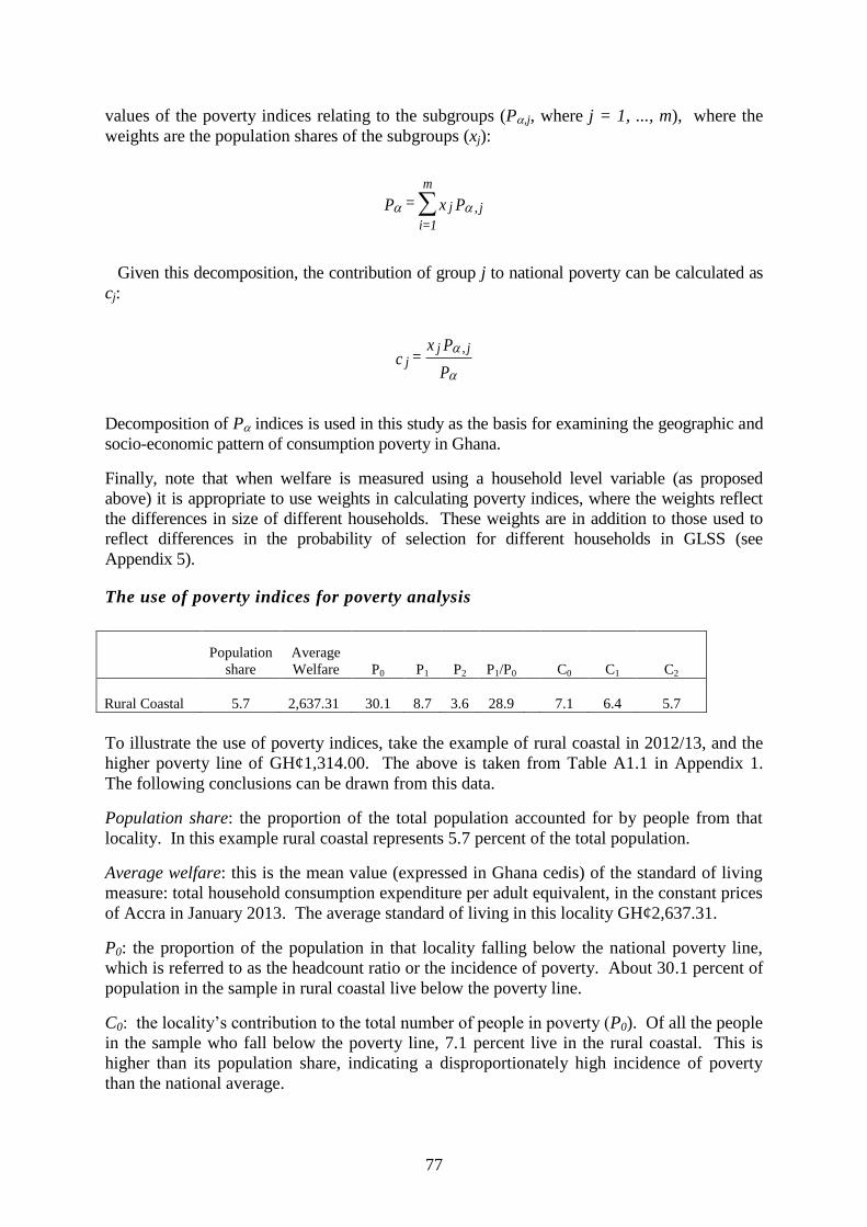
77
values of the poverty indices relating to the subgroups (P,j, where j = 1, ..., m), where the
weights are the population shares of the subgroups (xj):
Given this decomposition, the contribution of group j to national poverty can be calculated as
cj:
Decomposition of P indices is used in this study as the basis for examining the geographic and
socio-economic pattern of consumption poverty in Ghana.
Finally, note that when welfare is measured using a household level variable (as proposed
above) it is appropriate to use weights in calculating poverty indices, where the weights reflect
the differences in size of different households. These weights are in addition to those used to
reflect differences in the probability of selection for different households in GLSS (see
Appendix 5).
The use of poverty indices for poverty analysis
Population
share
Average
Welfare P0 P1 P2 P1/P0
C0 C1 C2
Rural Coastal 5.7
2,637.31 30.1 8.7 3.6 28.9
7.1 6.4 5.7
To illustrate the use of poverty indices, take the example of rural coastal in 2012/13, and the
higher poverty line of GH¢1,314.00. The above is taken from Table A1.1 in Appendix 1.
The following conclusions can be drawn from this data.
Population share: the proportion of the total population accounted for by people from that
locality. In this example rural coastal represents 5.7 percent of the total population.
Average welfare: this is the mean value (expressed in Ghana cedis) of the standard of living
measure: total household consumption expenditure per adult equivalent, in the constant prices
of Accra in January 2013. The average standard of living in this locality GH¢2,637.31.
P0: the proportion of the population in that locality falling below the national poverty line,
which is referred to as the headcount ratio or the incidence of poverty. About 30.1 percent of
population in the sample in rural coastal live below the poverty line.
C0: the locality’s contribution to the total number of people in poverty (P0). Of all the people
in the sample who fall below the poverty line, 7.1 percent live in the rural coastal. This is
higher than its population share, indicating a disproportionately high incidence of poverty
than the national average.
Px=P j,j
m
1=i
P
Px=c
j,jj

78
P1/P0: the income gap ratio or the depth of poverty. Those in the rural coastal below the
poverty line have an average standard of living 28.9 percent below the selected poverty line.
P1: the poverty gap index. This measure takes account of both the incidence and the depth of
poverty. It gives an indication of the minimum level of resources which would be required to
eliminate poverty, assuming that resources could be perfectly targeted to raise every poor
person exactly to the poverty line. The amount of money required is equivalent to 8.7 percent
of the poverty line for every person in rural coastal. This amount would then have to be
allocated, with perfect targeting, among those in rural coastal who are below the poverty line
in order to raise them exactly to the poverty line.
C1: the locality’s contribution to total poverty, as measured by the poverty index P1. C1 is
lower than C0 because there is a lower depth of poverty in the rural coastal than in the country
as a whole.
P2: the severity of poverty. This measure is more complex to interpret, but reflects the need
to give greater attention to the needs of the poorest. It takes account of the distribution of
poverty among the poor, giving greater weight to the poorest of the poor.
C2: The locality’s contribution to the severity of poverty, as measured by the poverty index
P2. C2 is lower than C1; as more emphasis is placed on the depth of poverty (moving from P0
to P1 to P2), the contribution of the rural coastal to severity of poverty in Ghana decreases.