PREDICTIVE MODELING: BASICS BEYOND · PREDICTIVE MODELING: BASICS & BEYOND | 2. Agenda 1. Review of...
115
www.scioinspire.com ©2011 SCIOinspire Corp. All rights reserved. November 2011 PREDICTIVE MODELING: BASICS & BEYOND
Transcript of PREDICTIVE MODELING: BASICS BEYOND · PREDICTIVE MODELING: BASICS & BEYOND | 2. Agenda 1. Review of...

| 1
www.scioinspire.com
©2011 SCIOinspire Corp. All rights reserved.
November 2011
PREDICTIVE MODELING: BASICS & BEYOND

| 2
Agenda
1. Review of the Basics.
2. Data, Data Preparation and Algorithms.
3. Grouper Models.
Break.
4. Uses of Predictive Models.
5. Types of predictive models.
Break
6. Practical Example of Model Building.
7. Applications – case studies.

| 33©2011 SCIOinspire Corp. Confidential and Proprietary. All rights reserved.
IntroductionsIntroductions
Author of several books and peer‐reviewed studies in healthcare management and
predictive modeling.
Published 2008
Published May 2011
Ian Duncan FSA FIA FCIA MAAA. Founder and former President, Solucia Consulting, A
SCIOinspire Company. Actuarial Consulting company founded in 1998. A leader in
managed care, disease management, predictive modeling applications and outcomes
evaluation. Now a visiting Professor at UC Santa Barbara and Adjunct Faculty at
Georgetown. Board member, Massachusetts Health Insurance Connector Authority.

| 44©2011 SCIOinspire Corp. Confidential and Proprietary. All rights reserved.
Predictive Modeling: A Review of the Basics

| 55©2011 SCIOinspire Corp. Confidential and Proprietary. All rights reserved.
Definition of RiskDefinition of Risk
• You can’t understand risk adjustment or predictive modeling without
understanding risk.
• At its most fundamental, risk is a combination of two factors: loss
and probability.
• We define a loss
as having occurred when an individual’s post‐
occurrence state is less favorable than the pre‐occurrence state.
Financial Risk is a function of Loss Amount and Probability, but
in
healthcare, risk and loss are not restricted to financial quantities
only. Therefore we use the following, more general, definition:
RISK = F (Loss; Probability)

| 66©2011 SCIOinspire Corp. Confidential and Proprietary. All rights reserved.
•Another way of saying this is that Risk is a function of Frequency
(of
occurrences) and Severity
of the occurrence.
•In healthcare, we are interested in many different states. Most
frequently actuaries are interested in Financial Loss, which occurs
because an event imposes a cost on an individual (or employer or
other
interested party). To a clinician, however, a loss could be a loss of
function, such as an inability to perform at a previous level or
deterioration in an organ.
RISK = F (Loss; Probability)
Definition of RiskDefinition of Risk

| 77©2011 SCIOinspire Corp. Confidential and Proprietary. All rights reserved.
•Predictive Modeling is the process of estimating, predicting or
stratifying members according to their relative risk.
• Prediction can be performed separately for Frequency
(probability) and Severity (loss).
•Risk adjustment is a concept closely related to Predictive Modeling.
One way to distinguish is in their uses: Predictive Modeling focuses on
the future; while Risk Adjustment often applies to the past.
Definition of Predictive ModelingDefinition of Predictive Modeling

| 88©2011 SCIOinspire Corp. Confidential and Proprietary. All rights reserved.
Typical Distribution of health costTypical Distribution of health cost
Health cost (Risk) is typically highly‐skewed. The challenge is to predict the tail*.
* Distribution of allowed charges within the Solucia Consulting database (multi‐million member national database).
| 99©2011 SCIOinspire Corp. Confidential and Proprietary. All rights reserved.
Key Concept: Member TransitionKey Concept: Member Transition
MEMBERSHIP
Baseline Year Sequent Year
Baseline Year Cost Group
Baseline
Percentage
Membership
LOW <$2,000
MODERATE
$2,000‐$24,999
HIGH
$25,000+
LOW
<$2,000
69.5% 57.4%11.7%
0.4%MODERATE
$2,000‐$24,999
28.7% 9.9%17.7%
1.1%HIGH $25,000+
1.8% 0.2%0.9%
0.6%TOTAL 100.0% 67.6% 30.3% 2.2%

| 1010©2011 SCIOinspire Corp. Confidential and Proprietary. All rights reserved.
Key Concept: Member TransitionKey Concept: Member Transition
Baseline
Year
Sequent YearPMPY CLAIMS
Baseline
Year
Sequent Year
CLAIMS TREND
Baseline Year
Cost Group
Mean Per
Capita Cost
LOW
<$2,000
MODERATE
$2,000‐
$24,999
HIGH
$25,000+
Mean Per
Capita Cost
Trend
LOW
<$2,000
MODERATE
$2,000‐
$24,999
HIGH
$25,000+
LOW
<$2,000
$510.37 $453.24 11.5% 7.4%
$5,282.58 17.6%
$56,166.54 6.9%MODERATE
$2,000‐
$24,999
$6,157.06 $888.30 57.2% 2.5%
$6,803.91 34.1%
$49,701.87 15.8%HIGH
$25,000+
$55,197.12 $907.47 31.3% 0.1%
$10,435.51 2.7%
$73,164.49 13.0%TOTAL $518.72 $6,325.46 $57,754.19 100.0% 10.0% 54.4% 35.6%
AVERAGE $3,090.36 $3,520.09TREND 13.9%

| 1111©2011 SCIOinspire Corp. Confidential and Proprietary. All rights reserved.
Traditional (actuarial) Risk Prediction Traditional (actuarial) Risk Prediction
Age/Sex: although individuals of the same age and sex represent a range of
risk profiles and costs, groups
of individuals of the same age and sex
categories follow more predictable patterns of cost. The majority of non‐
Government healthcare is financed by employer groups.
Relative Cost PMPY by Age/SexMale Female Total
< 19 $1,429 $1,351 $1,39020‐29 $1,311 $2,734 $2,01730‐39 $1,737 $3,367 $2,56640‐49 $2,547 $3,641 $3,11650‐59 $4,368 $4,842 $4,60960‐64 $6,415 $6,346 $6,381Total $2,754 $3,420 $3,090

| 1212©2011 SCIOinspire Corp. Confidential and Proprietary. All rights reserved.
Typical Age/Sex Prediction (Manual Rating)Typical Age/Sex Prediction (Manual Rating)
Age/Sex: Relative costs for different age/sex categories can be expressed as
relative risk factors, enabling us to assess the “average”
risk of an
individual, or the overall (relative) risk of a population.
Relative Costs Using Age/Sex FactorsMale
Risk FactorMale
NumberFemale
Risk FactorFemaleNumber
WeightedNumber
< 19 0.46 4 0.44 12 7.1220‐29 0.42 12 0.88 19 22.0030‐39 0.56 24 1.09 21 36.3340‐49 0.82 30 1.18 24 52.9250‐59 1.41 15 1.57 12 39.9960‐64 2.08 3 2.05 1 8.29Total 0.89 88 1.11 89 166.65Total Membership 177.00
Relative age/sex factor 0.94

| 1313©2011 SCIOinspire Corp. Confidential and Proprietary. All rights reserved.
Accuracy of Traditional Risk Prediction Accuracy of Traditional Risk Prediction
Traditional (Age/Sex) risk prediction is somewhat accurate at the
population level. Larger group costs are more predictable than
smaller
groups. Demographic Factors as Predictors of Future Health Costs
Age/Sex Factors Factor RatioDifference**
(Predicted‐Actual)
EmployerNumberof lives Baseline
SubsequentYear
Subsequent/Average
PredictedCost*
ActualCost $ %
1 73 1.37 1.42 138% $4,853 $23,902 ($19,049) ‐392.5%2 478 0.74 0.76 74% $2,590 $2,693 ($102) ‐3.9%3 37 0.86 0.87 84% $2,965 $1,339 $1,626 54.8%4 371 0.95 0.97 95% $3,331 $3,325 $6 0.2%5 186 1.00 1.03 100% $3,516 $3,345 $170 4.8%6 19 1.80 1.85 180% $6,328 $10,711 ($4,383) ‐69.3%7 359 0.95 0.97 94% $3,315 $3,401 ($87) ‐2.6%8 543 0.94 0.96 93% $3,269 $3,667 ($398) ‐12.2%9 26 1.60 1.64 159% $5,595 $5,181 $414 7.4%
Average 1.00 1.03 1.00 $3,520 $3,520 $ ‐ 0.0%Sum of absolute Differences (9 sample groups only) $26,235

| 1414©2011 SCIOinspire Corp. Confidential and Proprietary. All rights reserved.
Prior Experience adds to accuracyPrior Experience adds to accuracy
To account for the variance observed in small populations, actuaries typically
incorporate prior cost into the prediction, which adds to the predictive accuracy.
A “credibility weighting”
is used. Here is a typical formula:
where
and N
is the number of members in the group.
Combination of Age, Sex, and Prior Cost as a Predictor of Future Experience.
Cost PMPY Difference vs. Actual
EmployerNo. oflives
Credibility
Factor Baseline
Subsequent
Year
Pre‐dicted Subsequent
Year Actual Difference
Difference(% of
Actual)1 73 0.19 $27,488 $9,908 $23,902 ($13,994) ‐141.2%2 478 0.49 $1,027 $2,792 $2,693 $100 3.6%3 37 0.14 $1,050 $2,724 $1,339 $1,385 50.9%4 371 0.43 $2,493 $3,119 $3,325 ($205) ‐6.6%5 186 0.30 $3,377 $3,617 $3,345 $271 7.5%6 19 0.10 $11,352 $6,971 $10,711 ($3,739) ‐63.6%7 359 0.42 $2,008 $2,880 $3,401 ($522) ‐18.1%8 543 0.52 $2,598 $3,108 $3,667 ($559) ‐18.0%9 26 0.11 $3,022 $5,350 $5,181 $169 3.2%…. …. …. …. …. …. …. ….
Average $3,090 $3,520 $3,520 $ 0 0%
Sum of absolute Differences (9 sample groups only) $20,944

| 1515©2011 SCIOinspire Corp. Confidential and Proprietary. All rights reserved.
What does Clinical information tell us about risk? What does Clinical information tell us about risk?
Having information about a patient’s condition, particularly chronic condition(s)
is potentially useful for predicting risk.
Condition‐Based Vs. Standardized Costs
Member Age Sex ConditionActual Cost (Annual)
Standardized
Cost
(age/sex)
Condition‐Based
Cost/ Standardized
Cost (%)
1 25 M None $863 $1,311 66%2 55 F None $2,864 $4,842 59%3 45 M Diabetes $5,024 $2,547 197%4 55 F Diabetes $6,991 $4,842 144%
5 40 MDiabetes and Heart
conditions
$23,479 $2,547 922%
6 40 M Heart condition $18,185 $2,547 714%
7 40 FBreast Cancer and
other conditions
$28,904 $3,641 794%
8 60 FBreast Cancer and
other conditions
$15,935 $6,346 251%
9 50 MLung Cancer and other
conditions
$41,709 $4,368 955%

| 1616©2011 SCIOinspire Corp. Confidential and Proprietary. All rights reserved.
Risk Groupers predict relative riskRisk Groupers predict relative risk
Commercial Risk Groupers are available that predict relative risk based on
diagnoses. Particularly helpful for small groups.
Application of Condition Based Relative Risk
Cost PMPYDifference
(Predicted‐Actual)
EmployerNumber of lives
Relative Risk Score Predicted Actual $ %
1 73 8.02 $28,214 $23,902 $4,312 15.3%2 478 0.93 $3,260 $2,693 $568 17.4%3 37 0.47 $1,665 $1,339 $326 19.6%4 371 0.94 $3,300 $3,325 ($25) ‐0.8%5 186 1.01 $3,567 $3,345 $222 6.2%6 19 4.14 $14,560 $10,711 $3,850 26.4%7 359 0.84 $2,970 $3,401 ($432) ‐14.5%8 543 0.80 $2,833 $3,667 ($834) ‐29.4%9 26 1.03 $3,631 $5,181 ($1,550) ‐42.7%
Average $ ‐ 0.0% $ ‐ 0.0%Sum of absolute Differences (9 sample groups only) $12,118

| 1717©2011 SCIOinspire Corp. Confidential and Proprietary. All rights reserved.
Condition and Risk Identification Condition and Risk Identification –– How?How?
•
At the heart of predictive modeling!
•
Who?
•
What common characteristics?
•
What are the implications of those characteristics?
•
There are many different algorithms for identifying member
conditions. THERE IS NO SINGLE AGREED FORMULA.
•
Condition identification often requires careful balancing of
sensitivity and specificity.

| 1818©2011 SCIOinspire Corp. Confidential and Proprietary. All rights reserved.
Identification Identification –– example (Diabetes)example (Diabetes)
Diabetics can be identified in different ways:
Diagnosis type Reliability Practicality
Physician Referral/ Medical Records/EMRs
High Low
Lab tests High Low
Claims Medium High
Prescription Drugs Medium High
Self-reported Low/medium Low
Medical and Drug Claims are often the most practical method of
identifying candidates for predictive modeling.

| 1919©2011 SCIOinspire Corp. Confidential and Proprietary. All rights reserved.
19
Identification Identification –– example (Diabetes)example (Diabetes)
ICD-9-CM CODE
DIABETES
DESCRIPTION
250.xx Diabetes mellitus
357.2 Polyneuropathy in diabetes
362.0, 362.0x Diabetic retinopathy
366.41 Diabetic cataract
648.00-648.04 Diabetes mellitus (as other current condiition in mother
classifiable elsewhere, but complicating pregnancy,
childbirth or the puerperioum.
Inpatient Hospital Claims – ICD‐9 Claims Codes

| 2020©2011 SCIOinspire Corp. Confidential and Proprietary. All rights reserved.
20
Diabetes Diabetes –– additional procedure codesadditional procedure codes
CODES
DIABETES;
CODE TYPE
DESCRIPTION - ADDITIONAL
G0108, G0109
HCPCS Diabetic outpatient self-management training services, individual or group
J1815 HCPCS Insulin injection, per 5 units
67227 CPT4 Destruction of extensive or progressive retinopathy, ( e.g. diabetic retinopathy) one or more sessions, cryotherapy, diathermy
67228 CPT4 Destruction of extensiive or progressive retinopathy, one or more sessions, photocoagulation (laser or xenon arc).
996.57 ICD-9-CM Mechanical complications, due to insulin pump
V45.85 ICD-9-CM Insulin pump status
V53.91 ICD-9-CM Fitting/adjustment of insulin pump, insulin pump titration
V65.46 ICD-9-CM Encounter for insulin pump training

| 2121©2011 SCIOinspire Corp. Confidential and Proprietary. All rights reserved.
Diabetes Diabetes –– drug codesdrug codes
Insulin or Oral Hypoglycemic Agents are often used to identify members. A
simple example follows; for more detail, see the HEDIS code‐set.
This approach is probably fine for Diabetes, but may not work for other
conditions where off‐label use is prevalent.
2710* Insulin**
2720* Sulfonylureas**2723* Antidiabetic - Amino Acid Derivatives**2725* Biguanides**2728* Meglitinide Analogues**2730* Diabetic Other**2740* ReductaseInhibitors**2750* Alpha-Glucosidase Inhibitors**2760* Insulin Sensitizing Agents**2799* Antiadiabetic Combinations**
OralAntiDiabetics
Insulin

| 2222©2011 SCIOinspire Corp. Confidential and Proprietary. All rights reserved.
Algorithm Development: Diabetes ExampleAlgorithm Development: Diabetes Example
Not all diabetics represent the same level of risk. Different diagnosis codes help
identify levels of severity.
Codes for Identification of Diabetes SeverityDiagnosis Code(ICD‐9‐CM) Code Description
250.0 Diabetes mellitus without mention of complication
250.1Diabetes
with
ketoacidosis
(complication
resulting
from
severe insulin deficiency)
250.2Diabetes
with
hyperosmolarity
(hyperglycemia
(high
blood sugar levels) and dehydration)
250.3 Diabetes with other coma
250.4Diabetes
with
renal
manifestations
(kidney
disease
and
kidney function impairment)
250.5 Diabetes with ophthalmic manifestations
250.6Diabetes with neurological manifestations (nerve damage
as a result of hyperglycemia)
250.7 Diabetes with peripheral circulatory disorders250.8 Diabetes with other specified manifestations250.9 Diabetes with unspecified complication

| 2323©2011 SCIOinspire Corp. Confidential and Proprietary. All rights reserved.
Algorithm Development: Diabetes ExampleAlgorithm Development: Diabetes ExampleRelative Costs of Members with Different Diabetes Diagnoses
Diagnosis CodeICD‐9‐CM
DescriptionAverage cost
PMPY
Relative
cost
250 A diabetes diagnosis without a fourth digit (i.e., 250 only). $13,258 105%250.0 Diabetes mellitus without mention of complication $10,641 85%
250.1Diabetes with ketoacidosis (complication resulting from
severe insulin deficiency)
$16,823 134%
250.2Diabetes with hyperosmolarity (hyperglycemia (high blood
sugar levels) and dehydration)
$26,225 208%
250.3 Diabetes with other coma $19,447 154%
250.4Diabetes with renal manifestations (kidney disease and
kidney function impairment)
$24,494 195%
250.5 Diabetes with ophthalmic manifestations $11,834 94%
250.6Diabetes with neurological manifestations (nerve damage
as a result of hyperglycemia)
$17,511 139%
250.7 Diabetes with peripheral circulatory disorders $19,376 154%250.8 Diabetes with other specified manifestations $31,323 249%250.9 Diabetes with unspecified complication $13,495 107%357.2 Polyneuropathy in Diabetes $19,799 157%362 Other retinal disorders $13,412 107%
366.41 Diabetic Cataract $13,755 109%
648Diabetes mellitus of mother complicating pregnancy
childbirth or the puerperium unspecified as to episode of
care
$12,099 96%
TOTAL $12,589 100%

| 2424©2011 SCIOinspire Corp. Confidential and Proprietary. All rights reserved.
Algorithm Development: Diabetes ExampleAlgorithm Development: Diabetes Example
Which leads to a possible relative risk severity structure for diabetes:
A Possible Code Grouping System for Diabetes
Severity Level Diagnosis Codes Included Average Cost Relative Cost
1 250; 250.0 $10,664 85%
2 250.5; 250.9; 362; 366.41; 648 $12,492 99%
3250.1; 250.3; 250.6; 250.7;
357.2
$18,267 145%
4 250.2; 250.4 $24,621 196%
5 250.8 $31,323 249%
TOTAL
(All diabetes codes) $12,589 100%

| 2525©2011 SCIOinspire Corp. Confidential and Proprietary. All rights reserved.
Risk GroupersRisk Groupers
Diagnoses found in claims are the “raw material”
of predictive
modeling.
Codes are required for payment, so they tend to be reasonably accurate
‐
providers have a vested interest in their accuracy.
Codes define important variables like Diagnosis (ICD‐9 or 10; HCPS; V
and G codes); Procedure (CPT); Diagnosis Group (DRG – Hospital); Drug
type/dose/manufacturer (NDC; J codes); lab test (LOINC); Place of
service, type of provider, etc. etc.
Identification Algorithms and “Grouper”
models sort‐through the raw
material and consolidate it into manageable like categories.

| 2626©2011 SCIOinspire Corp. Confidential and Proprietary. All rights reserved.
An important issue with any claims‐based identification algorithm is that you are
imputing, rather than observing a diagnosis. Thus you are always at risk of including
false positives, or excluding false negatives, from the analysis.
One consequence of using a grouper model is that you are at the mercy of the
modeler’s definition of diagnoses, and thus cannot control for false positives or
negatives.
All people are not equally identifiableAll people are not equally identifiable
Prevalence of Chronic Conditions Identified Using Different Claims AlgorithmsNumber of Claiming Events in the Year
Condition 4 or more 3 or more 2 or more 1 or moreAsthma 2.4% 2.9% 3.9% 6.1%Cardiovascular disease 0.8% 1.2% 1.7% 2.8%Heart Failure 0.2% 0.2% 0.3% 0.6%Pulmonary Disease 0.2% 0.3% 0.5% 1.0%Diabetes 3.3% 3.7% 4.1% 4.9%All 6.3% 7.4% 9.2% 13.1%
| 2727©2011 SCIOinspire Corp. Confidential and Proprietary. All rights reserved.
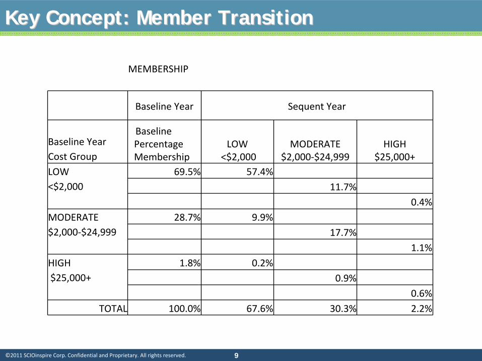
A less‐rigorous algorithm will identify more people with the condition (more
than twice as many in the example above). But it runs the risk of sweeping
in false positives. This table shows the likelihood re‐qualifying with the
condition in the following year:
All people are not equally identifiable (2)All people are not equally identifiable (2)
Probability that a Member Identified with Chronic Condition in Year 1 will be Identified with that Condition in Year 2
All Chronic Conditions
No. ClaimingEvents in Year 2
Number of Claiming Events in Year 1
4 or more 3 or more 2 or more 1 or more4 or more 59.7% 26.3% 15.7% 7.2%
3 or more 65.8% 35.9% 22.9% 10.6%
2 or more 72.0% 47.9% 34.3% 17.2%
1 or more 78.0% 62.3% 49.9% 30.9%
Do not re-qualify 22.0% 37.7% 50.1% 69.1%

| 2828©2011 SCIOinspire Corp. Confidential and Proprietary. All rights reserved.
Algorithm Development: Diabetes ExampleAlgorithm Development: Diabetes Example
Example of an identification algorithm:
Example of a Definitional Algorithm
Disease Type Frequency Codes
Diabetes Mellitus
Hospital Admission or ER visit
with diagnosis of diabetes in any
position
At least one event in a 12‐
month period
ICD‐9 codes 250, 357.2,
362.0, 366.41, 648.0
Professional visits with a
primary or secondary diagnosis
of diabetes
At least 2 visits in a twelve
month period
CPT Codes in range of
99200‐99499 series E & M
codes or 92 series for eye
visits
Outpatient Drugs: dispensed
insulin, hypoglycemic, or anti‐
hyperglycemic prescription drug
One or more prescriptions
in a twelve month period
Diabetes drugs (see HEDIS or
similar list of drug codes).
EXCLUDE
gestational
diabetes.
Any (as above) As above 648.8x

| 2929©2011 SCIOinspire Corp. Confidential and Proprietary. All rights reserved.
Sources of AlgorithmsSources of Algorithms
• NCQA – HEDIS.
• DMAA (Now CCA; Chronic definitions).
• Grouper Models.

| 3030©2011 SCIOinspire Corp. Confidential and Proprietary. All rights reserved.
Grouper ConstructionGrouper Construction
Grouper/Risk‐adjustment theory is based on a high correlation between risk scores
and actual dollars (resources used).
The Society of Actuaries has published three studies that test this correlation. They
are available from the SOA and are well worth reading. They explain some of the
theory of risk‐adjusters and their evaluation, as well as showing the correlation
between $’s and Risk Scores for a number of commercial models.
Note 1: the SOA tests both Concurrent (retrospective) and Prospective models.
Concurrent model correlations tend to be higher.
Note 2: there are some issues with models that you should be aware of:
• They tend to be less accurate at the “extremes”
(members with high or low risk
scores);
• We have observed an inverse correlation between risk‐score and $’s across a wide
range of members.

| 3131©2011 SCIOinspire Corp. Confidential and Proprietary. All rights reserved.
Commercial Groupers: SOA studiesCommercial Groupers: SOA studies
There have been three Society of Actuaries studies of commercial
risk grouper
models published. All are available at www.soa.org.
Dunn DL, Rosenblatt A, Taira DA, et al. "A comparative Analysis of Methods of
Health Risk Assessment." Society of Actuaries (SOA Monograph M‐HB96‐1).
Oct
1996:1‐88.
Cumming RB, Cameron BA, Derrick B, et al. "A Comparative Analysis of Claims‐
Based Methods of Health Risk Assessment for Commercial Populations".
Research study sponsored by Society of Actuaries.
2002.
Winkelman R, Mehmud S. "A Comparative Analysis of Claims‐Based Tools for
Health Risk Assessment".
Society of Actuaries.
2007 Apr:1‐63. (available at: www.soa.org/files/pdf/ risk‐assessmentc.pdf ).

| 3232©2011 SCIOinspire Corp. Confidential and Proprietary. All rights reserved.
Commercial Groupers: SOA studiesCommercial Groupers: SOA studies
The Society of Actuaries studies show:
1.Risk grouper modeling tools use different algorithms
to group the source data. For
example, the Symmetry models are built on episodes of care, DRGs
are built on hospital
episodes, while other models are built on diagnoses.
2.Similar performance among all leading risk groupers.
3.Accuracy of prediction has increased since the publication of the original study. In part,
this is due to more accurate coding and the inclusion of more claims codes.
4.Risk groupers use relatively limited data
sources (e.g. DCG and Rx Groups use ICD‐9 and
NDC codes but not lab results or HRA information).
5.Accuracy of retrospective (concurrent) models is now in the 30%‐40% R2
range.
Prospective
model accuracy is in the range of 20% to 25%.

| 3333©2011 SCIOinspire Corp. Confidential and Proprietary. All rights reserved.
A note about Prospective and Concurrent ModelsA note about Prospective and Concurrent Models
Both have their place. Neither is perfect.
1.Concurrent models are also called Retrospective.
The concurrent model is used to reproduce actual historical costs. This type of
model is used for assessing relative resource use and for determining compensation to
providers for services rendered because it normalizes costs across different members.
Normatively, the concurrent model provides an assessment of what
costs should have
been for members, given the health conditions with which they presented in the past
year. It is also used in program evaluation, which is performed once all known conditions
may be identified.
2.The Prospective model predicts what costs will be for a group of members in the future.
The Prospective model is predicting the unknown, because the period over which the
prediction is made lies in the future. The Concurrent model, by contrast, provides an
estimate of normalized costs for services that have already occurred. For prospective
prediction, members with no claims receive a relative risk score
component based on
age/sex alone.

| 3434©2011 SCIOinspire Corp. Confidential and Proprietary. All rights reserved.
A note about Prospective and Concurrent ModelsA note about Prospective and Concurrent Models
Concurrent models have the advantage that they represent all the
known information
about the member in the completed year. However, when they are used to compensate
providers (for example) for managing a group of members, there is a risk to the provider
that if the provider does a good job and prevents the exacerbation of the member’s
condition, the member risk score (and therefore the provider’s compensation) will be
lower than it would be if the provider does not prevent the exacerbation.
Prospective models are often used to allocate revenue to different managed care plans.
The drawback to this approach is that members’
prospective risk scores are based on
historical data, and do not take account of developing (incident) conditions that emerge
during the year.

| 3535©2011 SCIOinspire Corp. Confidential and Proprietary. All rights reserved.
CommerciallyCommercially--available Risk Groupersavailable Risk GroupersCommercially Available Grouper Models
Developer Risk Grouper Data Source
CMSDiagnostic Risk Groups (DRG) (There are a
number of subsequent “refinements”
to the
original DRG model.
Hospital claims only
CMS HCCs Age/Sex, ICD ‐9
3M Clinical Risk Groups (CRG)All Claims (inpatient, ambulatory
and drug)
IHCIS/Ingenix Impact ProAge/Sex, ICD‐9NDC, Lab
UC San DiegoChronic disability payment systemMedicaid Rx
Age/Sex, ICD ‐9NDC
Verisk Sightlines™DCGRxGroup
Age/Sex, ICD ‐9Age/Sex, NDC
Symmetry/IngenixEpisode Risk Groups (ERG)Pharmacy Risk Groups (PRG)
ICD – 9, NDCNDC
Symmetry/Ingenix Episode Treatment Groups (ETG) ICD – 9, NDC
Johns Hopkins Adjusted Clinical Groups (ACG) Age/Sex, ICD – 9

| 3636©2011 SCIOinspire Corp. Confidential and Proprietary. All rights reserved.
Grouper AlgorithmsGrouper Algorithms
As an alternative to commercially‐available risk groupers, analysts can develop
their own models using common data mining techniques. Each method has its
pros and cons:
There is a considerable amount of work involved in building algorithms from scratch, particularly
when this has to be done for the entire spectrum of diseases. Adding drug or laboratory sources to
the available data increases the complexity of development.
While the development
of a model may be within the scope and resources of the analyst
who is
performing research, use of models for production purposes (for risk adjustment of payments to a
health plan or provider groups for example) requires that a model be maintained to accommodate
new codes. New medical codes are not published frequently, but new drug codes are released
monthly, so a model that relies on drug codes will soon be out of date unless updated regularly.
Commercially‐available clinical grouper models are used extensively for risk adjustment when a
consistent model, accessible to many users, is required. Providers and plans, whose financial stability
relies on payments from a payer, often require that payments be made according to a model that is
available for review and validation.

| 3737©2011 SCIOinspire Corp. Confidential and Proprietary. All rights reserved.
Grouper AlgorithmsGrouper AlgorithmsAn analyst that builds his own algorithm for risk prediction has
control over
several factors that are not controllable with commercial models:
Which codes, out of the large number of available codes to recognize. The numbers of codes and their
redundancy (the same code will often be repeated numerous times in a member record) makes it
essential to develop an aggregation or summarization scheme.
The level at which to recognize the condition. How many different levels of severity should be
recognized?
The impact of co‐morbidities. Some conditions are often found together (for example heart disease
with diabetes). The analyst will need to decide whether to maintain separate conditions and then
combine where appropriate, or to create combinations of conditions.
The degree of certainty with which the diagnosis has been identified (confirmatory information). The
accuracy of a diagnosis may differ based on who codes the diagnosis, for what purpose and how
frequently a diagnosis code appears in the member record. The more frequently a diagnosis code
appears, the more reliable the interpretation of the diagnosis. Similarly, the source of the code
(hospital, physician, laboratory) will also affect the reliability of the diagnostic interpretation.
Data may come from different sources with a range of reliability
and acquisition cost. A diagnosis in a
medical record, assigned by a physician, will generally be highly reliable. Other types of data are not
always available or as reliable.

| 3838©2011 SCIOinspire Corp. Confidential and Proprietary. All rights reserved.
Example of Grouper ConstructionExample of Grouper Construction
Grouper models are constructed in a similar fashion to that illustrated
above. Below we show the hierarchical structure of the DxCG model for
Diabetes:
Aggregate Condition Category
Related Condition Category
Condition Category
DxGroup
Diabetes Co-Morbidity
Level
Traumatic dislocation of hip
Diabetes
Type I Diabetes
Diabetes with Acute
Complications
Diabetes with Renal
Manifestation
Diabetes with Neurologic or
Peripheral Circulatory
Manifestation
Diabetes with Ophtalmologic Manifestation
Diabetes with No or Unspecified Complications
DiabeticNeuropathy
Type I Diabetes with
Peripheral Circulatory Disorders
Type IDiabetes with Neurological
Manifestations
Type II Diabetes with Peripheral
Circulatory Disorders
Type II Diabetes with Neurological
Manifestations
ICD-9-CM xxxx xxxx xxxx
ACC
RCC
CC
DCG
ICD

| 3939©2011 SCIOinspire Corp. Confidential and Proprietary. All rights reserved.
Example of Grouper ConstructionExample of Grouper Construction
Grouper models are constructed in a similar fashion to that illustrated above.
Below we show how the risk score is developed for a patient with
diagnoses of
Diabetes, HTN, CHF and Drug Dependence, illustrating the hierarchical and
additive structure of the DxCG model:
Example of Construction of a Relative Risk Score
Condition Category Risk Score Contribution Notes
Diabetes with No orUnspecified Complications 0.0 Trumped by Diabetes with
Renal ManifestationDiabetes with Renal Manifestation 2.1
Hypertension 0.0 Trumped by CHFCongestive Heart Failure (CHF) 1.5
Drug Dependence 0.6Age-Sex 0.4Total Risk Score 4.6

| 4040©2011 SCIOinspire Corp. Confidential and Proprietary. All rights reserved.
Concurrent vs. Prospective ModelsConcurrent vs. Prospective Models
• An area that will receive more attention with Health Reform and Exchanges.• There are two major types of Grouper models: concurrent and prospective.
The concurrent model is used to reproduce actual historical costs. This type
of model is used for assessing relative resource use and for determining
compensation to providers for services rendered because it normalizes costs
across different members. Normatively, the concurrent model provides an
assessment of what costs should have been for members, given the
conditions with which they presented in the past year. • The Prospective model predicts what costs will be for a group of members in
the future. The Prospective model is predicting the unknown, because the
period over which the prediction is made lies in the future. The
Concurrent
model provides an estimate of normalized costs for services that
have
already occurred. For prospective prediction, members with no claims
receive a relative risk score component based on age/sex alone.

| 4141©2011 SCIOinspire Corp. Confidential and Proprietary. All rights reserved.
EpisodeEpisode‐‐based Groupersbased Groupers
Episode 467Depression Clean PeriodLook Back
Lab Prescription Office Visit Office Visit Office Visit
Hospital Admissions
An example of an episode Group: the Symmetry Grouper.

| 4242©2011 SCIOinspire Corp. Confidential and Proprietary. All rights reserved.
Construction of Relative Risk Scores Using ETGsExample: Male Aged 58
ETG Severity Level Description ERG Description Retrospective
Risk WeightsProspective
Risk Weights
163000 2 Diabetes 2.022 Diabetes w/significant complication/co-morbidity I 0.9874 1.2810
386800 1 Congestive HeartFailure 8.043 Ischemic heart disease, heart
failure, cardiomyopathy III 2.2870 2.0065
238800 3 Mood Disorder,Depression 4.033 Mood disorder, depression
w/ significant cc/cb 0.8200 0.7913
473800 3 Ulcer 11.022 Other moderate cost gastroenterology II 2.3972 0.6474
666700 1 Acne 17.011 Lower cost dermatology I 0.1409 0.1023
666700 1 Acne 17.011 Lower cost dermatology I
Demographic risk: Male 55-64 0.73316.6325 5.5616
−−−
Application of the Symmetry Grouper. Risk Scores are developed similarly to DxCG.
EpisodeEpisode‐‐based Groupersbased Groupers

| 4343©2011 SCIOinspire Corp. Confidential and Proprietary. All rights reserved.
One more very useful grouperOne more very useful grouper……
Example of Therapeutic Classes Within the GPI Structure
Group Class Sub Class Group Class Sub ClassGROUPS 1- 16 ANTI-INFECTIVE AGENTS
01 00 00 *PENICILLINS*01 10 00 Penicillin G
01 30 00 PENICILLINASE -RESISTANT PENICILLINS
01 50 00 AMINO PENICILLINS/BROAD SPECTRUM PENICILLINS
01 20 00 Ampicillins
01 40 00 EXTENDED SPECTRUM PENICILLINS
01 99 00 *Penicillin Combinations**01 99 50 *Penicillin-Arninoglycoside Combinations***01 99 40 *Penicillin-NSAIA Combinations***
02 00 00 *CEPHALOSPORINS *
02 10 00 *Cephalosporins -1st Generation**02 20 00 *Cephalosporins -2nd Generation**02 30 00 *Cephalosporins -3rd Generation**
02 40 00 *Cephalosporins -4th Generation**
02 99 00 *Cephalosporin Combinations**
03 00 00 *MACROLIDE ANTIBIOTICS*
03 10 00 *Erythromycins**03 10 99 *Erythromycin Combinations***03 20 00 *Troleandomycin**03 30 00 *Lincomycins**03 40 00 *Azithromycin**03 50 00 *Clarithromycin**03 52 00 *Dirithromycin**
Etc. Etc. Etc.
Drug groupers group 100,000s NDC codes into manageable therapeutic classes

| 4444©2011 SCIOinspire Corp. Confidential and Proprietary. All rights reserved.
RulesRules‐‐based vs. Statistical Modelsbased vs. Statistical Models
We are often asked about rules‐based models.
1.
First, all models ultimately have to be converted to rules in an
operational setting.
2.
What most people mean by “rules‐based models”
is actually a
“Delphi*”
approach. For example, application of “Gaps‐in‐care”
or
clinical rules (e.g. ActiveHealth).
3.
Rules‐based models have their place in Medical Management. One
challenge, however, is risk‐ranking identified targets, particularly
when combined with statistical models.
* Meaning that experts, , rather than statistics, determine the risk factors.

| 4545©2011 SCIOinspire Corp. Confidential and Proprietary. All rights reserved.
DonDon’’t overlook nont overlook non--conditioncondition--based Riskbased Risk
| 4646©2011 SCIOinspire Corp. Confidential and Proprietary. All rights reserved.
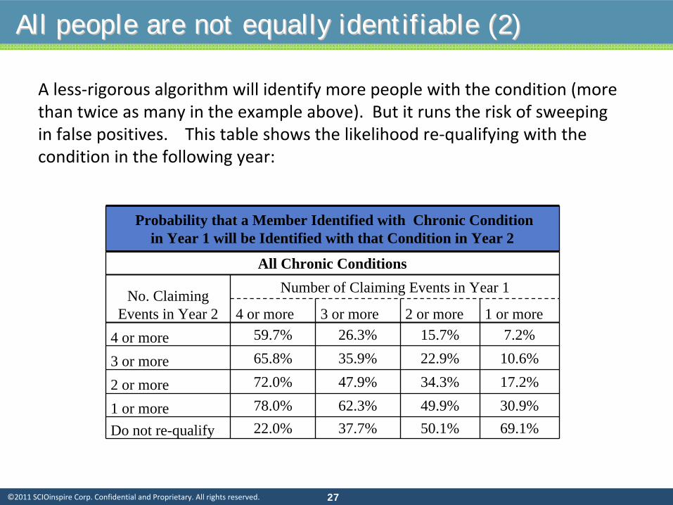
NonNon--conditioncondition--based Riskbased Risk
Relationship Between Modifiable Health Risk Factorsand Annual Health Insurance Claims

| 4747©2011 SCIOinspire Corp. Confidential and Proprietary. All rights reserved.
NonNon--conditioncondition--based Riskbased Risk

| 4848©2011 SCIOinspire Corp. Confidential and Proprietary. All rights reserved.
Developing your own modelDeveloping your own model
There are pros and cons to using a commercially available model.
There is no
reason not to develop your won predictive or risk adjustment model. Chapters
7‐12 of my book address different statistical models that are encountered in this
work. Examples of statistical models used frequently:
•Linear Regression. Advantage: everyone understands this. •Generalized linear model and Logistic regression: more sophisticated models
often used for healthcare data. •Tree models: more difficult to apply operationally than regression models. •Neural networks: black box.
There are a couple of others less frequently encountered.

| 4949©2011 SCIOinspire Corp. Confidential and Proprietary. All rights reserved.
Types of Statistical ModelsTypes of Statistical Models
Logistic Regression
Generalized Linear Models
Time Series
Survival Analysis
Non-linear Regression
Linear Regression
Decision Trees

| 5050©2011 SCIOinspire Corp. Confidential and Proprietary. All rights reserved.
Neural Network Genetic
Algorithms
Nearest Neighbor Pairings
Principal Component
AnalysisRule
Induction Kohonen Network
Fuzzy Logic
Bayes
Networks
Simulated Annealing
Artificial Intelligence ModelsArtificial Intelligence Models

| 5151©2011 SCIOinspire Corp. Confidential and Proprietary. All rights reserved.
Supervised learning (Predictive Modeling)
Neural Network
Fuzzy Logic
Decision Trees (rule Induction)
K‐Nearest Neighbor (KNN)
Etc.
Unsupervised Learning
Association Rules (rule induction)
Principal components analysis (PCA)
Kohonen Networks, also known as
Self‐Organizing Maps (SOM)
Cluster Analysis, etc.
Optimization or Search Methods:Conjugate
Gradient
Genetic algorithm
Simulated annealing
Etc.
Artificial Intelligence ModelsArtificial Intelligence Models

| 5252©2011 SCIOinspire Corp. Confidential and Proprietary. All rights reserved.
Some Quick CommentsSome Quick Comments
1.
Linear Regression remains popular because it is simple, effective and
practitioners understand it.
2.
Generalized Linear Models (GLM): in these models, the linear relationship
between the dependent and independent variables (basis of Linear
Models)
is relaxed, so the relationship can be non‐linear.
3.
Logistic Regression is one frequently used example of GLM in which
dependence may be discrete rather than continuous.
4.
Time Series models are models that are fitted to moving data.
5.
Decision Trees are a means of classifying a population using a series of
structured, successive steps.
6.
Non‐linear regression: models relationships that are non‐linear (often by
transforming data).
7.
Survival Analysis develops a “hazard rate”
or the probability that an
individual will experience the event at time t.

| 5353©2011 SCIOinspire Corp. Confidential and Proprietary. All rights reserved.
Practical Model Building

| 5454©2011 SCIOinspire Corp. Confidential and Proprietary. All rights reserved.
•
A model is a set of coefficients to be applied to production data in a
live environment.
•
With individual data, the result is often a predicted value or “score.”
For example, the likelihood that an individual will purchase something,
or will experience a high‐risk event (surrender; claim, etc.). (In
practical applications, individual scores are rolled‐up or averaged at
the population level.)
•
For underwriting, we can predict either cost or risk‐score. For care
management, the prediction could be cost or the likelihood of an
event.
Practical Model BuildingPractical Model Building
What is a Model??

| 5555©2011 SCIOinspire Corp. Confidential and Proprietary. All rights reserved.
Available data for creating the risk score included the following:
•
Eligibility/demographics
•
Rx claims
•
Medical claims
For this project, several data mining techniques were considered: neural net,
CHAID decision tree, and regression. The regression was chosen for the
following reasons:
• The regression model was more intuitively understandable by end‐
users than other models; and
• With proper data selection and transformation, the regression was
very effective, more so than the tree.
BackgroundBackground
| 5656©2011 SCIOinspire Corp. Confidential and Proprietary. All rights reserved.
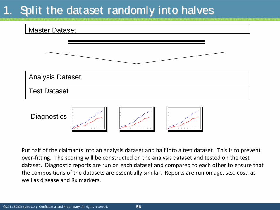
Test Dataset
Analysis Dataset
Master Dataset
Put half of the claimants into an analysis dataset and half into
a test dataset. This is to prevent
over‐fitting. The scoring will be constructed on the analysis dataset and tested on the test
dataset. Diagnostic reports are run on each dataset and compared to each other to ensure that
the compositions of the datasets are essentially similar. Reports are run on age, sex, cost, as
well as disease and Rx markers.
Diagnostics
1. Split the dataset randomly into halves1. Split the dataset randomly into halves

| 5757©2011 SCIOinspire Corp. Confidential and Proprietary. All rights reserved.
57
•
In any data‐mining project, the output is only as good as the input.
•
Most of the time and resources in a data mining project are
actually used for variable preparation and evaluation, rather than
generation of the actual “recipe”.
2. Build and Transform independent variables2. Build and Transform independent variables

| 5858©2011 SCIOinspire Corp. Confidential and Proprietary. All rights reserved.
3. Build dependent variable3. Build dependent variable
•
What are we trying to predict? Utilization? Cost? Likelihood of high cost?
•
A key step is the choice of dependent variable. What is the best choice?
•
A likely candidate is total patient cost in the predictive period. But total
cost has disadvantages:
•
It includes costs such as injury or maternity that are not generally
predictable.
•
It includes costs that are steady and predictable, independent of
health status (capitated expenses).
•
It may be affected by plan design or contracts.
•
So we could predict total cost (allowed charges) net of random costs and
capitated expenses.
•
Predicted cost can be converted to a risk‐factor.

| 5959©2011 SCIOinspire Corp. Confidential and Proprietary. All rights reserved.
Select promising variable
Check relationship with dependent variable
Transform variable to improve relationship
The process below is applied to variables from the baseline data.
Typical transforms include.
•
Truncating data ranges to minimized the effects of outliers.
•
Converting values into binary flag variables.
•
Altering the shape of the distribution with a log transform to compare
orders of magnitude.
•
Smoothing progression of independent variables
3. Build and transform Independent Variables3. Build and transform Independent Variables

| 6060©2011 SCIOinspire Corp. Confidential and Proprietary. All rights reserved.
•
A simple way to look at variables.
•
Convert to a discrete variable. Some variables such as number of
prescriptions are already discrete. Real‐valued variables, such as cost
variables, can be grouped into ranges.
•
Each value or range should have a significant portion of the patients.
•
Values or ranges should have an ascending or descending relationship with
average value of the composite dependent variable.
Typical
“transformed
variable”
3. Build and transform Independent Variables3. Build and transform Independent Variables
0
5
10
15
20
25
30
35
40
1 2 3 4
% Claimants
Avg of compositedependent variable

| 6161©2011 SCIOinspire Corp. Confidential and Proprietary. All rights reserved.
•
The following variables were most promising
•
Age ‐Truncated at 15 and 80
•
Baseline cost
•
Number of comorbid conditions truncated at 5
•
MClass
•
Medical claims‐only generalization of the comorbidity variable.
•
Composite variable that counts the number of distinct ICD9 ranges
for which the claimant has medical claims.
•
Ranges are defined to separate general disease/condition
categories.
•
Number of prescriptions truncated at 10
4. Select Independent Variables4. Select Independent Variables
| 6262©2011 SCIOinspire Corp. Confidential and Proprietary. All rights reserved.
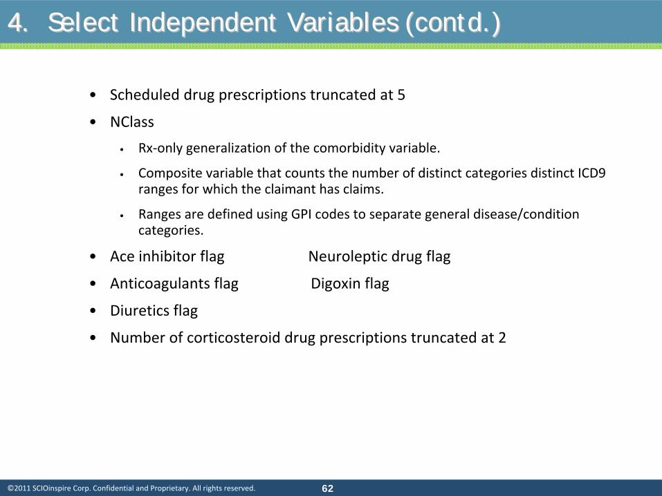
•
Scheduled drug prescriptions truncated at 5
•
NClass
•
Rx‐only generalization of the comorbidity variable.
•
Composite variable that counts the number of distinct categories
distinct ICD9
ranges for which the claimant has claims.
•
Ranges are defined using GPI codes to separate general disease/condition
categories.
•
Ace inhibitor flag Neuroleptic drug flag
•
Anticoagulants flag Digoxin flag
•
Diuretics flag
•
Number of corticosteroid drug prescriptions truncated at 2
4. Select Independent Variables (contd.)4. Select Independent Variables (contd.)

| 6363©2011 SCIOinspire Corp. Confidential and Proprietary. All rights reserved.
5. Run Stepwise Linear Regression5. Run Stepwise Linear Regression
An ordinary linear regression is simply a formula for determining a best‐
possible linear equation describing a dependent variable as a function of the
independent variables. But this pre‐supposes the selection of a best‐possible
set of independent variables. How is this best‐possible set of independent
variables chosen?
One method is a stepwise regression. This is an algorithm that determines
both a set of variables and a regression. Variables are selected in order
according to their contribution to incremental R2.

| 6464©2011 SCIOinspire Corp. Confidential and Proprietary. All rights reserved.
5. Run Stepwise Linear Regression (continued)5. Run Stepwise Linear Regression (continued)
Stepwise Algorithm
1. Run a single‐variable regression for each independent variable. Select the
variable that results in the greatest value of R2. This is “Variable 1”.
2. Run a two‐variable regression for each remaining independent variable. In
each regression, the other independent variable is Variable 1. Select the
remaining variable that results in the greatest incremental
value of R2. This
is “Variable 2.”
3. Run a three‐variable regression for each remaining independent variable.
In each regression, the other two independent variables are Variables 1 and
2. Select the remaining variable that results in the greatest incremental
value of R2. This is “Variable 3.”
……
n. Stop the process when the incremental value of R2
is below some pre‐
defined threshold.

| 6565©2011 SCIOinspire Corp. Confidential and Proprietary. All rights reserved.
6. Results 6. Results -- ExamplesExamples
•
Stepwise linear regressions were run using the "promising" independent
variables as inputs and the composite dependent variable as an output.
•
Separate regressions were run for each patient sex.
•
Sample Regressions
•
Female
Scheduled drug prescription
358.1
NClass
414.5
MClass
157.5
Baseline cost
0.5
Diabetes Dx
1,818.9
Intercept
18.5
Why are some variables selected while others are omitted? The stepwise algorithm favors variables that are relatively uncorrelated with previously-selected variables. The variables in the selections here are all relatively independent of each other.

| 6666©2011 SCIOinspire Corp. Confidential and Proprietary. All rights reserved.
6. Results 6. Results -- ExamplesExamples
• Examples of application of the female model
Female Regression Regression Formula
(Scheduled Drug *358.1) + (NClass*414.5) + (Cost*0.5) + (Diabetes*1818.9) + (MClass*157.5) -18.5
Raw ValueTransformed
Value Predicted Value Actual ValueClaimant
ID1 3 2 716.20$ Value Range RV< 2 2 < RV < 5 RV >52 2 2 716.20$ Transformed Value 1.0 2.0 3.03 0 1 358.10$
1 3 3 1,243.50$ Value Range RV < 2 2 < RV < 5 RV > 52 6 6 2,487.00$ Transformed Value 0.5 3.0 6.03 0 0.5 207.25$
1 423 2,000 1,000.00$ Value Range RV < 5k 5k < RV < 10k RV > 10k2 5,244 6,000 3,000.00$ Transformed Value 2,000 6,000 10,000 3 1,854 2,000 1,000.00$
1 0 0 -$ Value Range Yes No2 0 0 -$ Transformed Value 1.0 0.03 0 0 -$
1 8 3 472.50$ Value Range RV < 1 1 < RV < 7 RV > 72 3 2 315.00$ Transformed Value 0.5 2.0 3.03 0 0.5 78.75$
1 3,413.70$ 4,026.00$ 2 6,499.70$ 5,243.00$ 3 1,625.60$ 1,053.00$
MClass
Transform Function
Schedule Drugs
NClass
Cost
Diabetes
MClass
TOTAL
Schedule Drugs
NClass
Cost
Diabetes

| 6767©2011 SCIOinspire Corp. Confidential and Proprietary. All rights reserved.
In this section we will look at up to 5 different case studies,
depending on time.
1.
Underwriting model.
2.
Underwriting (group disability).
3.
Case management case identification.
4.
Wellness Prediction using Risk Factors.
5.
Health plan members with depression.
Model Evaluation: Case ExamplesModel Evaluation: Case Examples

| 6868©2011 SCIOinspire Corp. Confidential and Proprietary. All rights reserved.
•
Large client.
•
Several years of data provided for modeling.
•
Never able to become comfortable with data which did not perform
well according to our benchmark statistics ($/claimant; $PMPM;
number of claims per member).
Background Background –– Case 1Case 1
Client (excl.
capitation)
Claims/
Member/
Year PMPM Benchmark
Claims/
Member/
Year PMPM
Medical 14.4 $ 176.00
Rx 7.7 $ 41.23
Medical + Rx 5.36 $ 82.38 Medical + Rx 22.1 $ 217.23

| 6969©2011 SCIOinspire Corp. Confidential and Proprietary. All rights reserved.
•
Built models to predict cost in year 2 from year 1.
•
Now for the hard part: evaluating the results.
Background Background –– Case 1Case 1

| 7070©2011 SCIOinspire Corp. Confidential and Proprietary. All rights reserved.
How well does the model perform?How well does the model perform?
All Groups
0
20
40
60
80
100
120
140
-100%
+
-90% to
-99%
-80% to
-89%
-70% to
-79%
-60% to
-69%
-50% to
-59%
-40% to
-49%
-30% to
-39%
-20% to
-29%
-10% to
-19%
0% to
-9%
0% to
9%10
% to 19
%20
% to 29
%30
% to 39
%40
% to 49
%50
% to 59
%60
% to 69
%70
% to 79
%80
% to 89
%90
% to 99
%
Analysis 1: all groups. This analysis shows that, at the group
level, prediction is not
particularly accurate, with a significant number of groups at the extremes of the
distribution.

| 7171©2011 SCIOinspire Corp. Confidential and Proprietary. All rights reserved.
How well does the model perform?How well does the model perform?
Min 50 per group
0
10
20
30
40
50
60
-100%
+-90
% to -9
9%-80
% to -8
9%-70
% to -7
9%-60
% to -6
9%-50
% to -5
9%-40
% to -4
9%-30
% to -3
9%-20
% to -2
9%-10
% to -1
9%0%
to -9
%0%
to 9%
10% to
19%
20% to
29%
30% to
39%
40% to
49%
50% to
59%
60% to
69%
70% to
79%
80% to
89%
90% to
99%
Analysis 2: Omitting small groups (under 50 lives) significantly improves the actual/predicted
outcomes.
| 7272©2011 SCIOinspire Corp. Confidential and Proprietary. All rights reserved.
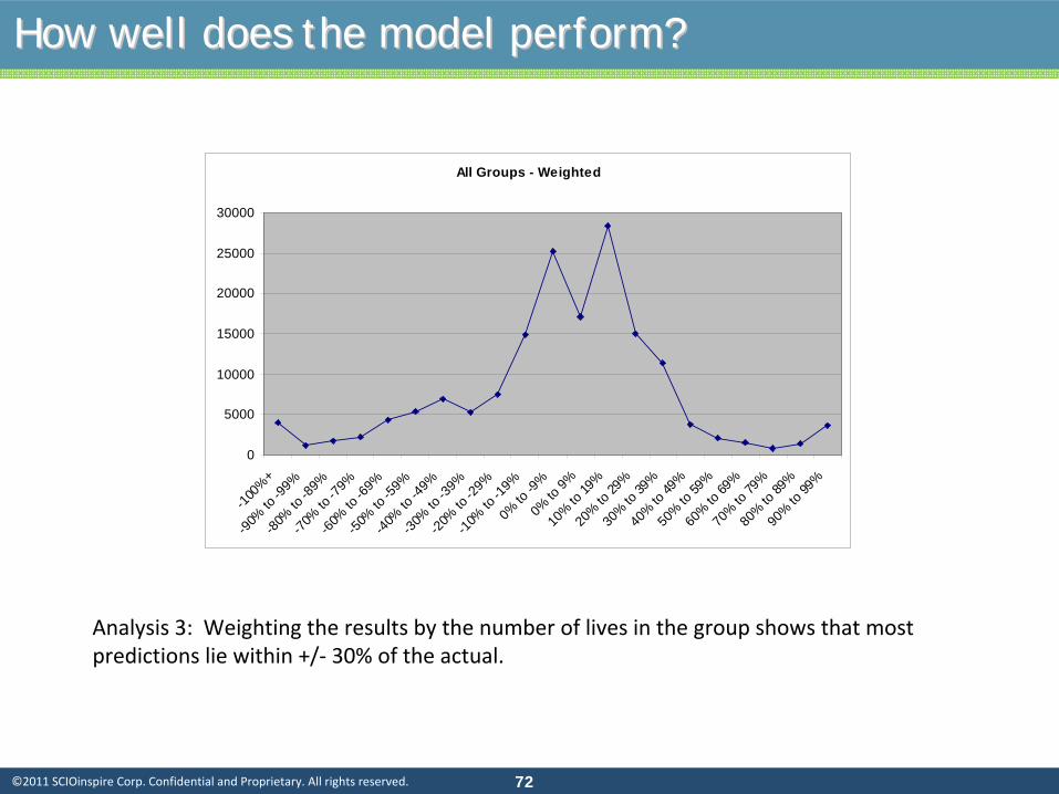
How well does the model perform?How well does the model perform?
All Groups - Weighted
0
5000
10000
15000
20000
25000
30000
-100%
+
-90% to
-99%
-80% to
-89%
-70% to
-79%
-60% to
-69%
-50% to
-59%
-40% to
-49%
-30% to
-39%
-20% to
-29%
-10% to
-19%
0% to
-9%
0% to
9%10
% to 19
%20
% to 29
%30
% to 39
%40
% to 49
%50
% to 59
%60
% to 69
%70
% to 79
%80
% to 89
%90
% to 99
%
Analysis 3: Weighting the results by the number of lives in the
group shows that most
predictions lie within +/‐
30% of the actual.

| 7373©2011 SCIOinspire Corp. Confidential and Proprietary. All rights reserved.
•
Significant data issues were identified and not resolved.
•
This was a large group carrier who had many groups “re‐
classified”
during the period. They were unable to provide
good data that “matched”
re‐classified groups to their
previous numbers.
•
Conclusion: if you are going to do anything in this area, be
sure you have good data.
ConclusionConclusion

| 7474©2011 SCIOinspire Corp. Confidential and Proprietary. All rights reserved.
•
Long‐term Disability coverage.
•
Client uses a manual rate basis for rating small cases. Client believes
that case selection/ assignment may result in case assignment to
rating classes that is not optimal.
•
A predictive model may add further accuracy to the class assignment
process and enable more accurate rating and underwriting to be
done.
Background Background –– Case 2.Case 2.

| 7575©2011 SCIOinspire Corp. Confidential and Proprietary. All rights reserved.
•
A number of different tree models were built (client specified use of
Tree Models).
•
Technically, an optimal model was chosen.
Problem: how to convince Underwriting that:
•
Adding the predictive model to the underwriting process produces
more accurate results; and
•
They need to change their processes to incorporate the predictive
model.
BackgroundBackground

| 7676©2011 SCIOinspire Corp. Confidential and Proprietary. All rights reserved.
Some dataSome data
NodePREDICTED
Average Profit
PREDICTED Number in
Node
PREDICTED Number in Node
(Adjusted)
ACTUAL Number in
nodeACTUAL
Average Profit1 (3.03) 70 173 170 (0.60) 2 0.19 860 2,122 2,430 0.07 3 (0.20) 2,080 5,131 6,090 (0.06) 4 0.09 910 2,245 2,580 0.10 5 (0.40) 680 1,678 20 0.02 6 (0.27) 350 863 760 0.16 7 0.11 650 1,604 1,810 0.04 8 0.53 190 469 470 (0.01) 9 (0.13) 1,150 2,837 2,910 0.03
10 0.27 1,360 3,355 3,740 0.04 11 0.38 1,560 3,849 3,920 (0.07) 12 0.08 320 789 830 0.08 13 0.06 12,250 30,221 29,520 0.02 14 0.27 2,400 5,921 6,410 0.21 15 (1.07) 540 1,332 1,320 (0.03) 16 0.07 10,070 24,843 24,950 (0.08) 17 (0.33) 1,400 3,454 3,250 (0.10) 18 0.11 4,460 11,003 11,100 0.08 19 (0.13) 1,010 2,492 2,100 (0.11)
42,310 104,380 104,380 0.005

| 7777©2011 SCIOinspire Corp. Confidential and Proprietary. All rights reserved.
How well does the model perform?How well does the model perform?
NodePREDICTED
Average Profit
PREDICTED Number in
Node
PREDICTED Number in Node
(Adjusted)
ACTUAL Number in
nodeACTUAL
Average Profit
Directionally Correct (+ or -)
1 (3.03) 70 173 170 (0.60) 2 0.19 860 2,122 2,430 0.07 3 (0.20) 2,080 5,131 6,090 (0.06) 4 0.09 910 2,245 2,580 0.10 5 (0.40) 680 1,678 20 0.02 6 (0.27) 350 863 760 0.16 7 0.11 650 1,604 1,810 0.04 8 0.53 190 469 470 (0.01) 9 (0.13) 1,150 2,837 2,910 0.03
10 0.27 1,360 3,355 3,740 0.04 11 0.38 1,560 3,849 3,920 (0.07) 12 0.08 320 789 830 0.08 13 0.06 12,250 30,221 29,520 0.02 14 0.27 2,400 5,921 6,410 0.21 15 (1.07) 540 1,332 1,320 (0.03) 16 0.07 10,070 24,843 24,950 (0.08) 17 (0.33) 1,400 3,454 3,250 (0.10) 18 0.11 4,460 11,003 11,100 0.08 19 (0.13) 1,010 2,492 2,100 (0.11)
42,310 104,380 104,380 0.005 6 red13 green

| 7878©2011 SCIOinspire Corp. Confidential and Proprietary. All rights reserved.
How well does the model perform?How well does the model perform?
NodePREDICTED
Average Profit
PREDICTED Number in
Node
PREDICTED Number in Node
(Adjusted)
ACTUAL Number in
nodeACTUAL
Average Profit
Directionally Correct (+ or -)
Predicted to be
Profitable1 (3.03) 70 173 170 (0.60) 2 0.19 860 2,122 2,430 0.07 3 (0.20) 2,080 5,131 6,090 (0.06) 4 0.09 910 2,245 2,580 0.10 5 (0.40) 680 1,678 20 0.02 6 (0.27) 350 863 760 0.16 7 0.11 650 1,604 1,810 0.04 8 0.53 190 469 470 (0.01) 9 (0.13) 1,150 2,837 2,910 0.03
10 0.27 1,360 3,355 3,740 0.04 11 0.38 1,560 3,849 3,920 (0.07) 12 0.08 320 789 830 0.08 13 0.06 12,250 30,221 29,520 0.02 14 0.27 2,400 5,921 6,410 0.21 15 (1.07) 540 1,332 1,320 (0.03) 16 0.07 10,070 24,843 24,950 (0.08) 17 (0.33) 1,400 3,454 3,250 (0.10) 18 0.11 4,460 11,003 11,100 0.08 19 (0.13) 1,010 2,492 2,100 (0.11)
42,310 104,380 104,380 0.005 6 red13 green 11 nodes

| 7979©2011 SCIOinspire Corp. Confidential and Proprietary. All rights reserved.
Supporting Underwriting DecisionSupporting Underwriting Decision--makingmaking
Underwriting Decision Total Profit Average Profit per
Case
Cases Written
Accept all cases as rated. 557.5 0.005 104,380

| 8080©2011 SCIOinspire Corp. Confidential and Proprietary. All rights reserved.
Supporting Underwriting DecisionSupporting Underwriting Decision--makingmaking
Underwriting Decision Total Profit Average Profit per
Case
Cases Written
Accept all cases as rated. 557.5 0.005 104,380
Accept all cases predicted to be profitable; reject all predicted unprofitable cases.
1,379.4 0.016 87,760

| 8181©2011 SCIOinspire Corp. Confidential and Proprietary. All rights reserved.
Supporting Underwriting DecisionSupporting Underwriting Decision--makingmaking
Underwriting Decision Total Profit Average Profit per
Case
Cases Written
Accept all cases as rated. 557.5 0.005 104,380
Accept all cases predicted to be profitable; reject all predicted unprofitable cases.
1,379.4 0.016 87,760
Accept all cases predicted to be profitable; rate all cases predicted to be unprofitable +10%.
2,219.5 0.021 104,380

| 8282©2011 SCIOinspire Corp. Confidential and Proprietary. All rights reserved.
Supporting Underwriting DecisionSupporting Underwriting Decision--makingmaking
Underwriting Decision Total Profit Average Profit per
Case
Cases Written
Accept all cases as rated. 557.5 0.005 104,380
Accept all cases predicted to be profitable; reject all predicted unprofitable cases.
1,379.4 0.016 87,760
Accept all cases predicted to be profitable; rate all cases predicted to be unprofitable +10%.
2,219.5 0.021 104,380
Accept all cases for which the directional prediction is correct.
2,543.5 0.026 100,620

| 8383©2011 SCIOinspire Corp. Confidential and Proprietary. All rights reserved.
Supporting Underwriting DecisionSupporting Underwriting Decision--makingmaking
Underwriting Decision Total Profit Average Profit per
Case
Cases Written
Accept all cases as rated. 557.5 0.005 104,380
Accept all cases predicted to be profitable; reject all predicted unprofitable cases.
1,379.4 0.016 87,760
Accept all cases predicted to be profitable; rate all cases predicted to be unprofitable +10%.
2,219.5 0.021 104,380
Accept all cases for which the directional prediction is correct.
2,543.5 0.026 100,620
Accept all cases for which the directional prediction is correct; rate predicted unprofitable cases by +10%
3,836.5 0.038 100,620

| 8484©2011 SCIOinspire Corp. Confidential and Proprietary. All rights reserved.
Supporting Underwriting DecisionSupporting Underwriting Decision--makingmaking
Underwriting Decision Total Profit Average Profit per
Case
Cases Written
Accept all cases as rated. 557.5 0.005 104,380
Accept all cases predicted to be profitable; reject all predicted unprofitable cases.
1,379.4 0.016 87,760
Accept all cases predicted to be profitable; rate all cases predicted to be unprofitable +10%.
2,219.5 0.021 104,380
Accept all cases for which the directional prediction is correct.
2,543.5 0.026 100,620
Accept all cases for which the directional prediction is correct; rate predicted unprofitable cases by +10%
3,836.5 0.038 100,620
Accept all cases for which the directional prediction is correct.
2,540.8 0.025 101,090

| 8585©2011 SCIOinspire Corp. Confidential and Proprietary. All rights reserved.
Example 3: evaluating a highExample 3: evaluating a high--risk modelrisk model

| 8686©2011 SCIOinspire Corp. Confidential and Proprietary. All rights reserved.
•
Large health plan client seeking a model to improve case
identification for case management.
•
Considered two commercially‐available models:
•
Version 1: vendor’s typical predictive model based on
conditions only. Model is more typically used for risk‐
adjustment (producing equivalent populations).
•
Version 2: vendor’s high‐risk predictive model that predicts
the probability of a member having an event in the next 6‐
12 months.
BackgroundBackground

| 8787©2011 SCIOinspire Corp. Confidential and Proprietary. All rights reserved.
AnalysisAnalysis
•
Two models: standard, off‐the‐shelf grouper model vs. a model
developed specifically for predicting high‐risk individuals for case
management.
•
Client initially rejected model 2 as not adding sufficient value
compared with model 1. (Vendor’s pricing strategy was to charge
additional fees for model 2) based on cumulative predictions.

| 8888©2011 SCIOinspire Corp. Confidential and Proprietary. All rights reserved.
0.0% 10.0% 20.0% 30.0% 40.0% 50.0% 60.0% 70.0% 80.0% 90.0%
100.0%
99 96 93 90 87 84 81 78 75 72 69 66 63 60 57 54 51 48 45 42 39 36 33 30 27 24 21 18 15 12 9 6 3 0
Model Percentile
Percent of Members w/ Hospitalization Identified
Model 2 Model 1
Lift Chart – Comparison between Two models
AnalysisAnalysis

| 8989©2011 SCIOinspire Corp. Confidential and Proprietary. All rights reserved.
AnalysisAnalysis
•
Looking at the results over a narrower range, they appear different.

| 9090©2011 SCIOinspire Corp. Confidential and Proprietary. All rights reserved.
BackgroundBackground
0.0%
10.0%
20.0%
30.0%
40.0%
50.0%
60.0%
99 98 97 96 95 94 93 92 91 90 89 88 87 86 85 84 83 82 81 80
Model Percentile
Percent of Members w/ Hospitalization Identified
Model 2 Model 1
Lift Chart – Comparison between Two models
| 9191©2011 SCIOinspire Corp. Confidential and Proprietary. All rights reserved.
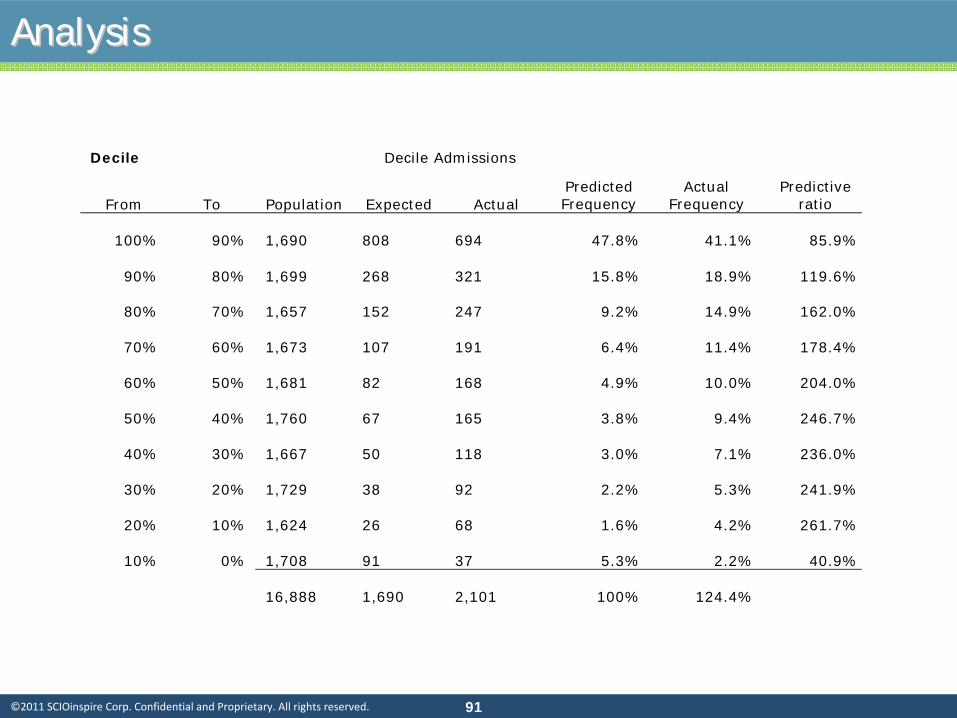
AnalysisAnalysis
Decile Decile Admissions
From To Population Expected Actual Predicted Frequency
Actual Frequency
Predictive ratio
100% 90% 1,690
808
694 47.8% 41.1% 85.9%
90% 80% 1,699
268
321 15.8% 18.9% 119.6%
80% 70% 1,657
152
247 9.2% 14.9% 162.0%
70% 60% 1,673
107
191 6.4% 11.4% 178.4%
60% 50% 1,681
82
168 4.9% 10.0% 204.0%
50% 40% 1,760
67
165 3.8% 9.4% 246.7%
40% 30% 1,667
50
118 3.0% 7.1% 236.0%
30% 20% 1,729
38
92 2.2% 5.3% 241.9%
20% 10% 1,624
26
68 1.6% 4.2% 261.7%
10% 0% 1,708
91
37 5.3% 2.2% 40.9%
16,888
1,690
2,101 100% 124.4%

| 9292©2011 SCIOinspire Corp. Confidential and Proprietary. All rights reserved.
Example 4: Constructing a Wellness ModelExample 4: Constructing a Wellness Model
| 9393©2011 SCIOinspire Corp. Confidential and Proprietary. All rights reserved.
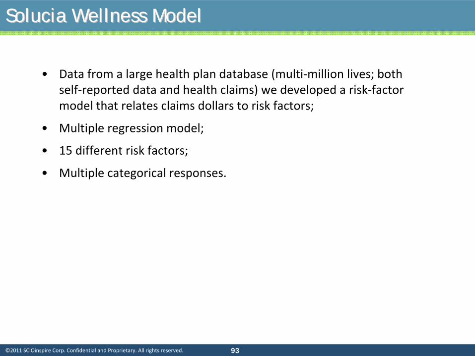
Solucia Wellness ModelSolucia Wellness Model
•
Data from a large health plan database (multi‐million lives; both
self‐reported data and health claims) we developed a risk‐factor
model that relates claims dollars to risk factors;
•
Multiple regression model;
•
15 different risk factors;
•
Multiple categorical responses.

| 9494©2011 SCIOinspire Corp. Confidential and Proprietary. All rights reserved.
Solucia Wellness ModelSolucia Wellness Model
Attribute Variable ValuesCost
Impact
Intercept 1 190
Personal Disease History 1
Chronic Obstructive Pulmonary Disease (COPD), Congestive Heart Failure (CHF), Coronary Heart Disease (CHD), Peripheral Vascular Disease (PVD) and Stroke 0 (No) -
1 (Yes) 10,553
Health ScreeningsHave you had a SIGMOIDOSCOPY within the last 5 years? (tube inserted in rectum to check for lower intestine problems) 0 (No) -
1 (Yes) 2,045 Weight Management Body Mass Index 26 (Min) 3,069
40 (No Value) 4,722 45 (Max) 5,312
Health Screenings Influenza (flu) within the last 12 months? 0 (No) -1 (Yes) 1,176
Personal Disease History 2
Have you never been diagnosed with any of the following: list of 27 major conditions 0 (No) -
1 (Yes) (1,220)
Personal Disease History 3
TIA (mini-stroke lasting less than 24 hrs), Heart Attack, Angina, Breast Cancer, Emphysema 0 (No) -
1 (Yes) 2,589 Immunizations Pneumonia 0 (No) -
1 (Yes) 1,118
Physical Activity 1Moderate-intensity physical activity - minutes per day 0 (Min, No Value)
-20 (Max)
(915)
Stress and Well- Being
In the last month, how often have you been angered because of things that happened that were outside your control?
0 (Never, Almost Never, Sometimes,
Fairly Often)
-
1 (Very Often, No Value) 1,632

| 9595©2011 SCIOinspire Corp. Confidential and Proprietary. All rights reserved.
Solucia Wellness ModelSolucia Wellness ModelSkin Protection
Please rate how confident you are that you can have your skin checked by a doctor once a year? 1 (Not at all confident) (224)
2 (Not confident) (447)
3 (Fairly confident) (671)4 (Confident) (894)
5 (Very Confident) (1,118)7 (No Value) (1,565)
Women's health 1Are you currently on hormone replacement therapy (Estrogen Therapy, Premarin) or planning to start? 0 (No) -
1 (Yes) 999
Women's health 2 Select the appropriate answer regarding pregnancy status/plan
1 (NotPlanning (I am planning on becoming pregnant in the next 6
months.)) 590 2 (No Value) 1,181
3 (Planning (I am planning on becoming pregnant in the next 6
months.)) 1,771 4 (Pregnant (I am
currently pregnant)) 2,361
Physical Activity 2 HIGH intensity activities? (hours per week) 0 (Min, No Value) -3 (Max) (917)
NutritionOn a typical day, how many servings do you eat of whole grain or enriched bread, cereal, rice, and pasta? 0 (None, No Value) -
1 (OneThree, FourFive) (868)2 (SixPlus) (1,736)
Tobacco Please rate how confident you are that you can keep from smoking cigarettes when you feel you need a lift. 1 (Not at all confident) (294)
1.5 (No Value) (441)
2 (Not confident) (588)
3 (Fairly confident) (883)4 (Confident) (1,177)
| 9696©2011 SCIOinspire Corp. Confidential and Proprietary. All rights reserved.
Example 5: Model to predict severe depressionExample 5: Model to predict severe depression

| 9797©2011 SCIOinspire Corp. Confidential and Proprietary. All rights reserved.
OBJECTIVES
To develop a depression prediction model based on available data
from the Solucia warehouse (primarily demographic and claims ).
Model objective is to identify those members of health plans who
are likely to register a high score on the PHQ‐9 survey when tested
by the depression survey.
To allow model users to apply the model to an entire unscreened
population and to identify those that are predicted to have a high
level of PHQ‐9 score.
5. Depression Model5. Depression Model

| 9898©2011 SCIOinspire Corp. Confidential and Proprietary. All rights reserved.
Study PopulationStudy Population
To develop the model we used a subset of members of our dataset for
whom a PHQ‐9 score exists.
All the members for this analysis are members of a large regional health
plan, enrolled between July 2004 and March 2008.
In total, 838 members were enrolled in the plan and completed
depression surveys between July 2004 and March 2008. A minority of
members completed multiple surveys.
Among those members with PHQ‐9 scores, 460 members had scores of
at least 10 on their first survey.
To validate the model we used a subset of members from another large
regional health plan , enrolled between July 2004 and March 2008.
In total, 193 members were enrolled in the plan and completed
depression surveys between July 2004 and March 2008.
Among those members with PHQ‐9 scores, 59 members had scores of at
least 10 on their first survey.

| 9999©2011 SCIOinspire Corp. Confidential and Proprietary. All rights reserved.
Available DataAvailable Data
Demographics: age, gender, zip code, ethnicity.
Eligibility: coverage periods, benefit information.
Medical claims: facility and professional.
Pharmacy claims.
PHQ‐9 scores.

| 100100©2011 SCIOinspire Corp. Confidential and Proprietary. All rights reserved.
Model DevelopmentModel Development
Note that the purpose of the model is not to predict cost or utilization.
The model simply predicts a binary outcome (presence/absence of a
PHQ‐9 score greater than or equal to 10).
Depression status defined by PHQ‐9 score >=10. Used first PHQ‐9
survey for members with multiple surveys.
Considered all claims incurred in the 12‐month period prior to PHQ‐9
survey date for independent variables.
We added a “disease burden”
or risk component by calculating a
concurrent risk score using a standard Solucia model.

| 101101©2011 SCIOinspire Corp. Confidential and Proprietary. All rights reserved.
Descriptive StatisticsDescriptive Statistics
PHQ-9 Score >=10
(N=460)
PHQ-9 Score <10(N=378)
Total(N=838)
Average age 41.9 44.1 42.9
Female (%) 37.2% 37.0% 37.1%
Average depression outpatient claims 14.17 3.70 9.45Proportion of members who had at least one depression outpatient claim 55.2% 20.6% 39.6%Proportion of members who had at least two fills of anti-depressants 67.4% 39.9% 55.0%Proportion of members who had at least one fill of anti-depressants 74.1% 47.4% 62.1%Proportion of members who had at least one fill of pain drug 62.8% 49.2% 56.7%
Average Solucia concurrent risk score 1.03 0.87 0.96Proportion of members who had at least one fatigue claim 13.7% 6.1% 10.0%
Average psychotherapy visits 67.0% 38.4% 54.1%
Proportion of males between 0 and 34 years old 15.9% 18.3% 16.9%

| 102102©2011 SCIOinspire Corp. Confidential and Proprietary. All rights reserved.
Predictive ModelingPredictive Modeling
Multivariate Logistic Models
Forward selection.
A split sample approach (50%/50%).
Key validation statistics: Area under ROC curve, sensitivity, and
specificity.
Internal validation: Model performance based on validation
sample.

| 103103©2011 SCIOinspire Corp. Confidential and Proprietary. All rights reserved.
Logistic ModelsLogistic Models
Dependent Variable: PHQ‐9 score is greater than or equal to 10.
Independent variables:
Measures from claims and demographics, plus Solucia concurrent risk score.
Development Group
Validation Group
Total
Members (n)419 419 838
Members without depression claims253 253 506
Members without anti-depressant scripts167 151 318
Members without both claims and scripts145 135 280
Members with PHQ-9 Score >=10217 243 460

| 104104©2011 SCIOinspire Corp. Confidential and Proprietary. All rights reserved.
Model Development SummaryModel Development Summary
Parameters Association Odds Ratio
Intercept Negative 0.39
Depression Outpatient Claims Positive 1.03
Depression Inpatient Claims Positive 1.59
Depression Drug 2fills Flag Positive 2.16
Pain Drug Flag Positive 1.13
Solucia Concurrent Risk Score Positive 1.29
Fatigue Flag Positive 2.43
Psychotherapy Visits Positive 1.02
Schizophrenia Positive 1.80
Age Positive 1.01Interaction between Concurrent RiskScore and Depression Outpatient Claims Negative 0.99Interaction between Concurrent Risk Score and Age Negative 0.99

| 105105©2011 SCIOinspire Corp. Confidential and Proprietary. All rights reserved.
Parameters Association Odds Ratio
Intercept Negative 0.33
Depression Drug 2 fills Flag Positive 1.59
Solucia Concurrent Risk Score Positive 2.60
Fatigue Flag Positive 2.62
Psychotherapy Visits Positive 1.02
Age Positive 1.01Interaction between Concurrent Risk Score and Age Negative 0.97
Model Development Summary (w/out Claims)Model Development Summary (w/out Claims)

| 106106©2011 SCIOinspire Corp. Confidential and Proprietary. All rights reserved.
Performance AssessmentPerformance Assessment
Receiver Operating Characteristic (ROC) curve:
Definition: A graphical representation of the trade off between the
false negative and false positive rates for every possible cut off.
By tradition, the plot shows the false positive rate (1‐specificity) on
the X axis and the true positive rate (sensitivity or 1 ‐
the false
negative rate) on the Y axis.
Interpretation:
0.90‐1.00 = Excellent
0.80‐0.90 = Good
0.70‐0.80 = Fair
0.60‐0.70 = Poor
0.50‐0.60 = Fail

| 107107©2011 SCIOinspire Corp. Confidential and Proprietary. All rights reserved.
Model Evaluation: ROC CurveModel Evaluation: ROC Curve

| 108108©2011 SCIOinspire Corp. Confidential and Proprietary. All rights reserved.
Sensitivity and SpecificitySensitivity and Specificity
Sensitivity: Maximizing the number of depressed patients correctly identified (correctly
predicted depressed patients over total depressed patients)
Specificity: Minimizing the number of false positives
Sensitivity= Number of True Positives
Number of True Positives + Number of False Negatives
Specificity= Number of True Negatives
Number of True Negatives + Number of False Positives

| 109109©2011 SCIOinspire Corp. Confidential and Proprietary. All rights reserved.
Sensitivity/Specificity (Contd.)Sensitivity/Specificity (Contd.)
Cut Points
Probability Sensitivity False Negative
Specificity False Positive
1 95% 4% 96% 100% 0%2 74% 25% 75% 96% 4%3 61% 45% 55% 86% 14%
4 50% 67% 33% 70% 30%5 38% 74% 26% 55% 45%6 34% 85% 15% 42% 58%7 27% 100% 0% 4% 96%
Solucia Depression Prediction Model
As the sensitivity increases, the specificity drops, and vice‐versa.
Using "Cutpoint
1 or 2" means that a very small proportion of the depressed
patients will be identified.
Using "Cutpoint
6 or 7" means that almost all of the patients with depression
will be identified as depressed, but so will many without depression.
Cutpoint
4 does a much better job of balancing the need to maximize the true
positives and minimize the false positives.

| 110110©2011 SCIOinspire Corp. Confidential and Proprietary. All rights reserved.
Table for Table for CutpointCutpoint 44
Actual (PHQ-9)
Y N Total
Predicted
Y 146 61 207
N 71 141 212
Total 217 202 419
PPV =146/207 =71%
Specificity =141/202 =70%
Sensitivity =146/217 =67%
False Negative =71/217 =33%
False Positive =61/202 =30%

| 111111©2011 SCIOinspire Corp. Confidential and Proprietary. All rights reserved.
Sensitivity analyses for potential substitutes for high PHQ-9 score Indicator
Variable Probability SensitivityFalse
Negative SpecificityFalse
Positive
Area Under ROC
Depression Claim Flag 64% 80% 20% 50% 50% 0.653
Depression Drug Flag 64% 74% 26% 55% 45% 0.646
Multivariate Logistic Model 50% 67% 33% 70% 30% 0.737
In these analyses, PHQ‐9 score >=10 was used as a gold standard to test the
sensitivity and specificity of applying those variables above to
identify
depressed patients.
The Multivariate model does a much better job of distinguishing depressed
patients from non‐depressed patients as demonstrated by substantially lower
false negative rates.
Sensitivity/Specificity (Contd.)Sensitivity/Specificity (Contd.)

| 112112©2011 SCIOinspire Corp. Confidential and Proprietary. All rights reserved.
Evaluation of Depression Claim FlagEvaluation of Depression Claim Flag
Actual (PHQ-9)
Y N Total
Predicted(Depression
Claim)
Y 174 100 274
N 43 102 145
Total 217 202 419
PPV =174/274 64%
Specificity =102/202 50%
Sensitivity =174/217 80%
False Negative =43/217 20%
False Positive =100/202 50%

| 113113©2011 SCIOinspire Corp. Confidential and Proprietary. All rights reserved.
The claims‐based model is effective in predicting high PHQ‐9 score
(score>=10) claimants:
Claims‐based variables, especially those directly related to individuals’
past
depression history are significantly correlated with a high level of PHQ‐9 score.
In general, demographic variables are not very predicative.
After controlling covariance, members are more likely to be depressed as age
increases.
The claims‐based model can be applied to identifying high‐risk
depression candidates across the entire population:
Area under ROC curves is greater than 0.7, which indicates a fair predictive power.
We continue to try to obtain PHQ‐9 score data from clients for whom we also have
claims data. The increased sample size may further improve the predicative power
of the model.
Depression Model SummaryDepression Model Summary

| 114114©2011 SCIOinspire Corp. Confidential and Proprietary. All rights reserved.
Selected referencesSelected references
This is not an exhaustive bibliography. It is only a starting point for explorations.
Duncan, I. Healthcare Risk Adjustment and Predictive Modeling.
2011
Actex
Publication.
Shapiro, A.F. and Jain, L.C. (editors); Intelligent and Other Computational
Techniques in Insurance;
World Scientific Publishing Company; 2003.
Dove, Henry G., Duncan, Ian, and Robb, Arthur; A Prediction Model for
Targeting Low‐Cost, High‐Risk Members of Managed Care Organizations;
The American Journal of Managed Care, Vol
9 No 5, 2003
Berry, Michael J. A. and Linoff, Gordon; Data Mining Techniques for
Marketing, Sales and Customer Support; John Wiley and Sons, Inc; 2004
Montgomery, Douglas C., Peck, Elizabeth A., and Vining, G Geoffrey;
Introduction to Linear Regression Analysis; John Wiley and Sons, Inc; 2001
Kahneman, Daniel, Slovic, Paul, and Tversky
(editors); Judgment under
uncertainty: Heuristics and Biases;
Cambridge University Press; 1982.

| 115115©2011 SCIOinspire Corp. Confidential and Proprietary. All rights reserved.
Selected references (contd.)Selected references (contd.)
Dove, Henry G., Duncan, Ian, and others; Evaluating the Results of
Care Management Interventions: Comparative Analysis of Different
Outcomes Measures. The SOA study of DM evaluation, available on
the web‐site at
http://www.soa.org/professional‐interests/health/hlth‐evaluating‐
the‐results‐of‐care‐management‐interventions‐comparative‐analysis‐
of‐different‐outcomes‐measures‐claims.aspx
Also available as: “Managing and Evaluating Healthcare Intervention
Programs (2008). Actex
Publications.
Winkelman
R. and S. Ahmed. A comparative analysis of Claims Based
Methods of health risk assessment ofr
Commercial Populations. (2007
update to the SOA Risk‐Adjuster study.) Available from the SOA; the
2002 study is on the website at:
http://www.soa.org/files/pdf/_asset_id=2583046.pdf