Predictive Location Tracking in Cellular and in Ad Hoc...
29
Chapter 8 Predictive Location Tracking in Cellular and in Ad Hoc Wireless Networks Nikos Dimokas 1 , Dimitrios Katsaros 1,2 , Panayiotis Bozanis 2 , and Yannis Manolopoulos 1 1 Department of Informatics, Aristotle University of Thessaloniki, Thessaloniki, Greece 2 Department of Computer & Communication Engineering, University of Thessaly, Thessaly, Greece 8.1 Introduction 163 8.2 Predictive Location Tracking Techniques 166 8.3 Predictive Location Indexing Techniques 176 8.4 Conclusion 186 Acknowledgments 187 References 187 Predicting the future is mostly a matter of managing not to blink as you witness the present. —William Gibson 8.1 INTRODUCTION The proliferation of cellular and ad hoc networks and the penetration of Internet services are changing many aspects of ubiquitous mobile computing. Constantly increasing mobile client populations utilize diverse mobile devices to access the Mobile Intelligence. Edited by Laurence T. Yang Copyright © 2010 John Wiley & Sons, Inc. 163
Transcript of Predictive Location Tracking in Cellular and in Ad Hoc...
Chapter 8
Predictive Location Trackingin Cellular and in Ad HocWireless Networks
Nikos Dimokas1, Dimitrios Katsaros1,2, Panayiotis Bozanis2,and Yannis Manolopoulos1
1 Department of Informatics, Aristotle University of Thessaloniki, Thessaloniki, Greece2 Department of Computer & Communication Engineering, University of Thessaly,Thessaly, Greece
8.1 Introduction 1638.2 Predictive Location Tracking Techniques 1668.3 Predictive Location Indexing Techniques 1768.4 Conclusion 186Acknowledgments 187References 187
Predicting the future is mostly a matter of managing not to blink as you witness thepresent.
—William Gibson
8.1 INTRODUCTION
The proliferation of cellular and ad hoc networks and the penetration of Internetservices are changing many aspects of ubiquitous mobile computing. Constantlyincreasing mobile client populations utilize diverse mobile devices to access the
Mobile Intelligence. Edited by Laurence T. YangCopyright © 2010 John Wiley & Sons, Inc.
163
164 Predictive Location Tracking
wireless medium and various heterogeneous applications (e.g., streaming video, Web)are being developed to satisfy the eager client requirements. The realization of sucha demanding environment requires addressing many technical issues, related to radiomanagement, networking, data management, and so on.
Most of the challenging issues and problems in this area are due to the fact thatthe underlying environment is extremely resource-starving and inherently uncertain.For instance, the wireless communication channels are bandwidth-limited and errorprone. The uncertainty due to node (user) mobility has fundamental impacts, sinceit induces uncertainly in the network topology and hence causes problems in routingand in data delivery. Additionally, traffic load and resource demands in cellular and inad hoc wireless networks are also uncertain, depending a lot on the user trajectories.
In this harsh environment, seamless and ubiquitous connectivity is a fundamentalgoal. This goal calls for smart techniques for determining the current and futurelocation of a mobile. The ability to determine the mobile client’s (future) locationcan significantly improve the wireless network’s overall performance. Consider forinstance the handover procedure in cellular networks, which is directly related to thedesign of resource management algorithms in such infrastructured networks; suchresources could be bandwidth, MAC frames, packets. Instead of relying on reactiveapproaches, that is, allocating appropriate resources during the handover, we couldcome up with proactive approaches, that is, allocating resources before needed, so as tobypass, instead of correct, the negative effect of handover [28]. Additionally, methodslike the Shadow Cluster [31] could benefit from location prediction by refrainingfrom allocating resources to all neighboring cells; with the exploitation of predictionsinstead, they could allocate resources only to the most probable-to-move cells. Finally,location prediction could be exploited in sequential paging schemes [8] to reduce thecombined paging cost and also in techniques for call admission control [60].
Location prediction and tracking is useful not only in cellular networks, but alsoto other types of wireless networks, such as mobile ad hoc networks (MANETs). A[Q1]
mobile ad hoc network is a wireless network in which a set of mobile nodes withwireless connectivity form a temporary network without the existence and supportof any infrastructure, for example, base stations, or centralized administration, forexample, switching centers. Communication in an ad hoc network between any twonodes that are out of one another’s transmission range is achieved through interme-diate nodes, which relay messages to set up a communication channel between thetwo nodes. For a MANET node v wishing to communicate with another MANETnode u not within its transmission range, knowledge of the future position(s) of nodev could help reduce its energy consumption, by postponing its communication to u
until it reaches closer to it. Such a technique has been investigated in Ref. [9].
8.1.1 Preliminaries
The present chapter deals with the issue of predictive location tracking in cellularand in ad hoc wireless networks and examines this issue in two different settings.In Section 8.2, we assume a generic symbolic network topology model, like that
8.1 Introduction 165
introduced in Ref. [8], where the existence of “cells” is assumed. The cells neednot be hexagonal, but can be of arbitrary shape. The notion of a wireless cell is [Q2]
well established in cellular networks; in ad hoc networks can be defined in a similarmanner, if we overlay a grid of any type [9] over the area, inside which the mobilehosts of the wireless ad hoc network are roaming. In this setting, the positioning of amobile is performed at the level of a cell. In Section 8.3, we withdraw the assumptionof the existence of cells, and the position of each mobile host is determined by itsgeographic coordinates only.
Connectivity in the presence of mobility is a nontrivial task; the network has towork against the uncertainty created by the mobile’s freedom of movement. Thus, themanagement of mobility is of crucial importance. Depending on whether a mobileterminal is actively communicating or in standby mode, we differentiate between(a) in-session mobility management and (b) out-of-session mobility management.The former is widely known in cellular networks as handoff management and dealswith mechanisms by which calls and sessions are kept alive while the mobile host ismoving from cell to cell, thus changing its network point of attachment. In general,the procedure of handoff management is considered easier than the management ofthe latter case, which is known as location management or location tracking and isresponsible for keeping track of mobiles in standby mode.
The location tracking problem in generic wireless networks involves two proce-dures, namely paging and update. At the one extreme, one can come up with a proposalfor this problem with the aid of paging, which is performed by the system; on a call ar-rival, the network initiates a search for the sought mobile, by (simultaneously) pollingevery possible site where the mobile can be found. In the case of cellular networks,this is performed by the mobile switching center, which broadcasts a page messageover a special forward control channel via the base stations. All the mobiles listento this paging message, but only the target mobile responses over a reverse channel.In the worst case, the system may have to page each cell of the whole service area.Clearly, this approach involves excessive signaling traffic and, thus, is problematic.
At the other extreme, one can come up with a solution that demands from themobile to report every time it moves from one site (cell) to another. This reporting iscalled location registration and starts with an update message sent by the mobile overa reverse channel, which is then followed by some traffic that takes care of relateddatabase maintenance operations at the system’s side. Again, this approach may alsogenerate excessive signaling traffic if the mobile changes cells frequently and, thus,is impractical.
In real situations, location tracking is performed as a hybrid between these ex-treme approaches [47]. Although a lot of (reactive) location management methodshave been proposed, the issue of predictive (or proactive) location tracking has latelyreceived significant attention due to its potential to reduce or even eliminate the latencyassociated with location tracking. Moreover, there are situation where prediction ofmobiles’ movements, that will eventually lead to network disconnection, may forcespecific decisions related to routing. Examples of these decisions involve the routingprotocols that are suitable for highly mobile ad hoc networks and for delay-tolerantnetworks [62].

166 Predictive Location Tracking
In general, predictive location tracking techniques work by constructing a mobil-ity model for each mobile host that models the mobility history of the mobile. Clearly,the two notions are different; the former is probabilistic and extends to the future,whereas the latter is deterministic and refers to the past. Location prediction is relatedto the ability of the underlying network to record, learn, and subsequently predict themobile’s movements. The success of the prediction is presupposed and is boost bythe fact that mobile users exhibit some degree of regularity in their movement [8].A “smart” network can record the movement history and then construct a mobilitymodel for its clients. The real challenge involved in designing an effective and efficientpredictive location tracking method is to quantify the utility of the past in predictingthe future.
8.1.2 Chapter Organization
The purpose of this chapter is to provide an overview of techniques suitable for pre-dicting the future locations of mobile hosts in wireless networks. It concentrates ontwo different scenarios; according to the first scenario, the network coverage area ispartitioned in nonoverlapping regions (named cells) and the location tracking is per-formed at the level of cells; according to the second scenario, there is no such tilingto the coverage area and location tracking is performed at the level of geographicalcoordinates. The first part of the chapter (Section 8.2) deals with the first scenarioand introduces information-theoretic methods suitable for predicting the future loca-tions of mobiles. The second part of the chapter (Section 8.3) deals with the secondscenario and presents the issues related to indexing the positions of mobile hosts inorder to support predictive queries. For these two broad and significant issues, thechapter surveys, classifies, and compares the state-of-the-art solutions, by discussingthe critical issues and challenges of predictive location tracking in wireless networks.
8.2 PREDICTIVE LOCATION TRACKING TECHNIQUES
Owing to the uncertainty inherent in the mobile’s movements, we can consider themto be the outcome of an underlying stochastic process, which can be modeled usingestablished information-theoretic concepts and tools [34, 56]. The cornerstone workof Ref. [17] exhibited the possibility of using methods, which have traditionallybeen used for data compression (thus, characterized as “information-theoretic”), incarrying out prediction. Considering a symbolic network topology model [8], we canmodel the respective state space as a finite alphabet comprised of discrete symbols.The alphabet consists of all possible sites (cells) where the client has ever visited ormight visit (assuming that the number of cells in the coverage area is finite). Withthis transformation, we can exploit methods that have traditionally been used for datacompression (thus, characterized as “information-theoretic”) to carry out prediction.In the rest of this section, we elaborate on these methods.

8.2 Predictive Location Tracking Techniques 167
8.2.1 The Discrete Sequence Prediction Problem
In quantifying the utility of the past in predicting the future, a formal definitionof the problem is needed, which we provide in the following lines. Let � be analphabet, consisting of a finite number of symbols s1, s2, . . . , s|�|, where | · | standsfor the length/cardinality of its argument. A predictor, which is an algorithm used togenerate prediction models, accumulates sequences of the type ai = α1
i , α2i , . . . , α
nii ,
where αji ∈ �, ∀i, j and ni denotes the number of symbols comprising ai. Without
loss of generality, we can assume that all the knowledge of the predictor consistsof a single sequence a = α1, α2, . . . , αn. On the basis of a, the predictor’s goal isto construct a model that assigns probabilities for any future outcome given “some”past. Using the characterization of the mobility model as a stochastic process (Xt)t∈N ,we can formulate the aforementioned goal as follows.
Definition 8.1 (Discrete Sequence Prediction Problem). At any given time instancet (meaning that t symbols xt, xt−1, . . . , x1 have appeared, in reverse order) calculatethe conditional probability
P[Xt+1 = xt+1|Xt = xt,Xt−1 = xt−1, . . .],
where xi ∈ �, ∀xt+1 ∈ �. This model introduces a stationary Markov chain, sincethe probabilities are not time-dependent. The outcome of the predictor is a rankingof the symbols according to their P . The predictors that use such kind of predictionmodels are termed Markov predictors.
Depending on the application, the predictor may return only the symbol(s), withthe highest probability, that is, implementing a “most-probable” prediction policy,or the symbols with the m highest probabilities, that is, implementing a “top-m”prediction policy, where m is an administratively set parameter. In any case, theselection of the policy is a minor issue and will not be considered in this chapter,which is only concerned with methods for inferring the ranking.
The “history” xt, xt−1, . . . used in the above definition is called the context of thepredictor and refers to the portion of the past that influences the next outcome. The his-tory’s length (also, called the length or memory or order of the Markov chain/predictor)will be denoted by l. Therefore, a predictor that exploits l past symbols will calculateconditional probabilities of the form
P[Xt+1 = xt+1|Xt = xt,Xt−1 = xt−1, . . . ,Xt−l+1 = xt−l+1]. (8.1)
Some Markov predictors fix, in advance of the model creation, the value of l,presetting it in a constant k in order to reduce the size and complexity of the predictionmodel. These predictors and the respective Markov chains are termed fixed lengthMarkov chains/predictors of order k. Therefore, they compute probabilities of theform:
P[Xt+1 = xt+1|Xt = xt,Xt−1 = xt−1, . . . ,Xt−k+1 = xt−k+1]. (8.2)
where k is a constant.

168 Predictive Location Tracking
Although it is a nice model from a probabilistic point of view, these Markov chainsare not very appropriate from the estimation point of view. Their main limitation isrelated to their structural poverty, since there is no means to set an optimized valuefor k.
Other Markov predictors deviate from the fixed memory assumption and allowthe order of the predictor to be of variable length, that is, to be a function of the valuesfrom the past.
P[Xt+1 = xt+1|Xt = xt,Xt−1 = xt−1, . . . ,Xt−l+1 = xt−l+1], (8.3)
where l = l(xt, xt−1, . . .).These predictors are termed variable length Markov chains; the length l might
range from 1 to t. If l = l(xt, xt−1, . . .) ≡ k for all xt, xt−1, . . ., then we obtain thefixed-length Markov chain. The variable length Markov predictors may or may notimpose an upper bound on the considered length. The concept of variable memoryoffers a richness in the prediction model and the ability to adjust itself to the datadistribution. If we can choose in a data driven way the function l = l(·), then we canonly gain with respect to the ordinary fixed-length Markov chains, but this is not astraightforward problem.
The Markov predictors (fixed or variable length) base their probability calcula-tions P on counts of the number of appearances of symbols after contexts. They alsotake special care to deal with the cases of unobserved symbols (i.e., symbols withzero appearance counts after contexts), assigning to them some “minimum probabilitymass.”
8.2.2 The Power of Markov Predictors
The issue of prediction in wireless networks, especially location prediction, has re-ceived attention during the past years, and the most important proposed techniquesfocus on the notions of learning automata, Kalman filtering, and pattern matching.
Learning automata are finite-state adaptive systems that interact continuouslywith their environment learning a “behavior.” Learning automata have been used inlocation prediction [28], and, although simple, they are not considered very efficientlearners because of the need to devise appropriate penatly/reward policies, which isusually done in an ad hoc way, and their slow convergence to the correct actions.
Kalman filtering is a recursive processing algorithm for producing optimal es-timates. Kalman filtering-based methods [33] construct a mobile motion equationrelying on specific distributions for its velocity, acceleration, and direction of move-ment. Therefore, they assume relatively accurate geographic position knowledge viasignal strength measurements. Their performance largely depends on the stabilizationtime of the Kalman filter and knowledge (or estimation) of the system’s parameters.
Finally, (approximate) pattern matching techniques have been used for locationprediction [33]. They compile (or assume existence of) aggregate or per-user mobil-ity profiles and perform approximate similarity matching between the current and thestored trajectories. The similarity matching is carried out through the computation
8.2 Predictive Location Tracking Techniques 169
of the edit distance between the current and each stored trajectory in order to derivepredictions. Although edit distance computation can be performed quite fast withdynamic programming, it is relatively hard to select the meaningful set of edit op-erations on the individual symbols (i.e., insert, delete, substitute), to assign weightson them, deal with unequal sequences of symbols, and select as similarity metric theedit distance instead of string alignment.
Consequently, a couple of questions arise regarding (a) why Markov predictorsare more appropriate for carrying out location prediction from the technical viewpointand (b) whether location prediction is amenable to Markovian prediction. Severaltechnical reasons advocate the use of Markov predictors in these problems, but theirmost profound advantage is their generality; they are domain-independent withoutany coupling to geographic coordinates or particular assumptions on distributions. Asimple mapping from the “entities” of the investigated domain to an alphabet is allthat is required. Thus, they are able to support location prediction.
Markovian prediction relies on the short memory principle, which, simply stated,says that the (empirical) probability distribution of the next symbol, given the pre-ceding sequence, can be quite accurately approximated by observing no more thanthe last few symbols in that sequence. This principle fits reasonably and intuitivelywith how humans are acting when travelling or seeking information. A mobile userusually travels with a specific destination in mind, designing its travel via specificroutes (roads or preferred pedestrian paths). This “targeted” traveling is far from arandom walk assumption and is confirmed by studies with real mobility traces [45].Therefore, the power of Markovian prediction stems from its generality and modelingcapability and also from its natural accordance with the human behavior.
8.2.3 Families of Markov Predictors
Markov predictors create probabilistic models for their input sequence(s) and usedigital search trees (tries) to keep track of the contexts of interest, along with somecounts used in the calculation of the conditional probabilities P . The root node ofthe trie corresponds to the “null” event/symbol, whereas every other node of the treecorresponds to a sequence of events; the sequence is used to label the node. Wewill consider a Markov predictor to be equivalent to its respective trie. Each node isaccompanied by a counter, which depicts how many times this event has appearedafter the sequence of events corresponding to the path from the root to the node’sfather has been observed.
For our convenience, we present some definitions useful in the sequel of thechapter. We use the sample sequence of events a = aabacbbabbacbbc. The length ofa is the number of symbols it contains, that is, |a| = 15. The appearance count ofsubsequence s = ab is E(s) = E(ab) = 2 and the normalized appearance count of s isequal to E(s) divided by the maximum number of (possibly overlapping) occurrencesa subsequence of the same length could have, considering the a’s length, that is,En(s) = E(s)/(|a| − |s| + 1). The conditional probability of observing a symbol aftera given subsequence is defined as the number of times that symbol has shown up right
170 Predictive Location Tracking
after the given subsequence divided by the total number of times that the subsequencehas shown up all, followed by any symbol. Therefore, the conditional probability ofobserving the symbol b after the subsequence a will be denoted as P(b|a) and at isequal to P(b|a) = (E(ab))/(E(a)) = 0.4. In the rest of this section, we survey thefamilies of Markov predictors.
8.2.3.1 The Prediction by Partial Match Scheme
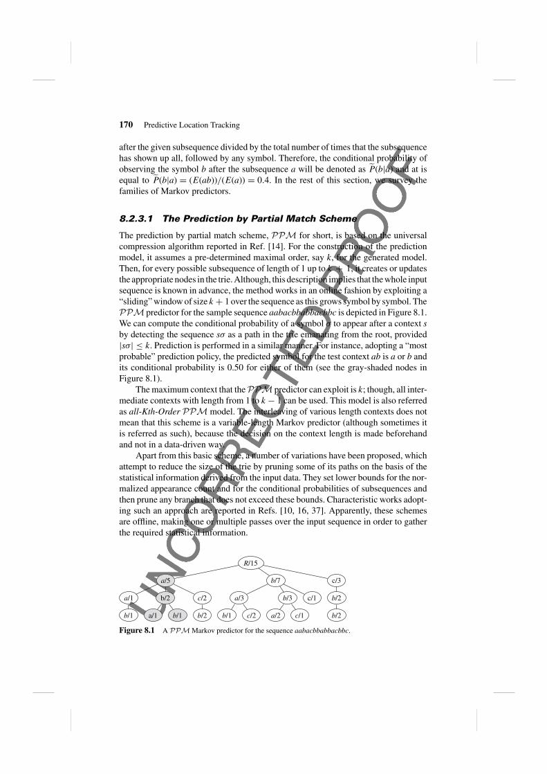
The prediction by partial match scheme, PPM for short, is based on the universalcompression algorithm reported in Ref. [14]. For the construction of the predictionmodel, it assumes a pre-determined maximal order, say k, for the generated model.Then, for every possible subsequence of length of 1 up to k + 1, it creates or updatesthe appropriate nodes in the trie. Although, this description implies that the whole inputsequence is known in advance, the method works in an online fashion by exploiting a“sliding” window of size k + 1 over the sequence as this grows symbol by symbol. ThePPM predictor for the sample sequence aabacbbabbacbbc is depicted in Figure 8.1.We can compute the conditional probability of a symbol σ to appear after a context s
by detecting the sequence sσ as a path in the trie emanating from the root, provided|sσ| ≤ k. Prediction is performed in a similar manner. For instance, adopting a “mostprobable” prediction policy, the predicted symbol for the test context ab is a or b andits conditional probability is 0.50 for either of them (see the gray-shaded nodes inFigure 8.1).
The maximum context that thePPM predictor can exploit is k; though, all inter-mediate contexts with length from 1 to k − 1 can be used. This model is also referredas all-Kth-Order PPM model. The interleaving of various length contexts does notmean that this scheme is a variable-length Markov predictor (although sometimes itis referred as such), because the decision on the context length is made beforehandand not in a data-driven way.
Apart from this basic scheme, a number of variations have been proposed, whichattempt to reduce the size of the trie by pruning some of its paths on the basis of thestatistical information derived from the input data. They set lower bounds for the nor-malized appearance count and for the conditional probabilities of subsequences andthen prune any branch that does not exceed these bounds. Characteristic works adopt-ing such an approach are reported in Refs. [10, 16, 37]. Apparently, these schemesare offline, making one or multiple passes over the input sequence in order to gatherthe required statistical information.
R/15
a/5
a/1
b/1
b/2
a/1 b/1
c/2
b/2
b/7
a/3
b/1 c/2
b/3
a/2 c/1
c/1
c/3
b/2
b/2
Figure 8.1 A PPM Markov predictor for the sequence aabacbbabbacbbc.
8.2 Predictive Location Tracking Techniques 171
8.2.3.2 The Lempel-Ziv-78 Scheme
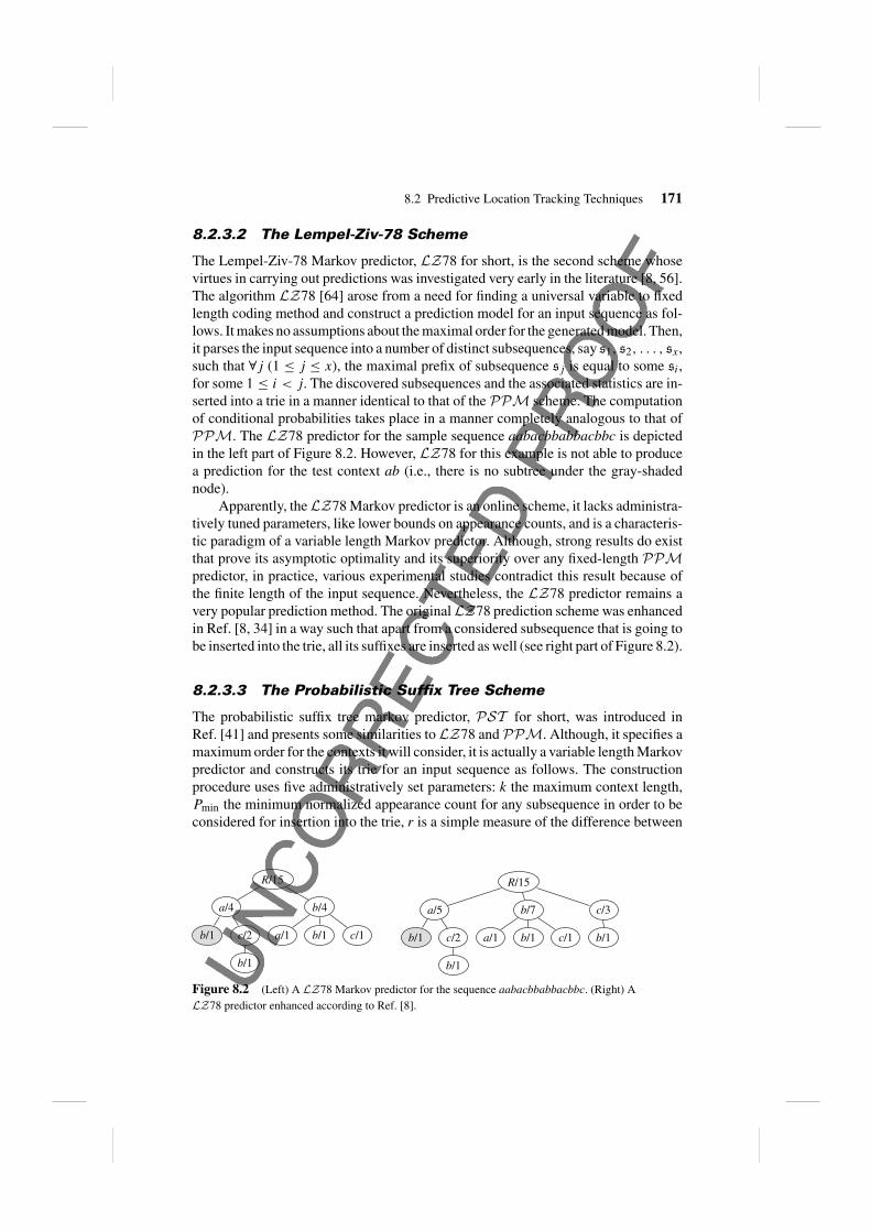
The Lempel-Ziv-78 Markov predictor, LZ78 for short, is the second scheme whosevirtues in carrying out predictions was investigated very early in the literature [8, 56].The algorithm LZ78 [64] arose from a need for finding a universal variable to fixedlength coding method and construct a prediction model for an input sequence as fol-lows. It makes no assumptions about the maximal order for the generated model. Then,it parses the input sequence into a number of distinct subsequences, say s1, s2, . . . , sx,such that ∀j (1 ≤ j ≤ x), the maximal prefix of subsequence sj is equal to some si,for some 1 ≤ i < j. The discovered subsequences and the associated statistics are in-serted into a trie in a manner identical to that of the PPM scheme. The computationof conditional probabilities takes place in a manner completely analogous to that ofPPM. The LZ78 predictor for the sample sequence aabacbbabbacbbc is depictedin the left part of Figure 8.2. However, LZ78 for this example is not able to producea prediction for the test context ab (i.e., there is no subtree under the gray-shadednode).
Apparently, the LZ78 Markov predictor is an online scheme, it lacks administra-tively tuned parameters, like lower bounds on appearance counts, and is a characteris-tic paradigm of a variable length Markov predictor. Although, strong results do existthat prove its asymptotic optimality and its superiority over any fixed-length PPMpredictor, in practice, various experimental studies contradict this result because ofthe finite length of the input sequence. Nevertheless, the LZ78 predictor remains avery popular prediction method. The original LZ78 prediction scheme was enhancedin Ref. [8, 34] in a way such that apart from a considered subsequence that is going tobe inserted into the trie, all its suffixes are inserted as well (see right part of Figure 8.2).
8.2.3.3 The Probabilistic Suffix Tree Scheme
The probabilistic suffix tree markov predictor, PST for short, was introduced inRef. [41] and presents some similarities to LZ78 and PPM. Although, it specifies amaximum order for the contexts it will consider, it is actually a variable length Markovpredictor and constructs its trie for an input sequence as follows. The constructionprocedure uses five administratively set parameters: k the maximum context length,Pmin the minimum normalized appearance count for any subsequence in order to beconsidered for insertion into the trie, r is a simple measure of the difference between
R/15
a/4
b/1 c/2
b/1
b/4
a/1 b/1 c/1
R/15
a/5
b/1 c/2
b/1
b/7
a/1 b/1 c/1
c/3
b/1
Figure 8.2 (Left) A LZ78 Markov predictor for the sequence aabacbbabbacbbc. (Right) ALZ78 predictor enhanced according to Ref. [8].
172 Predictive Location Tracking
R/13
a/5
b/2 c/2
b/2
b/7
a/3
c/2
b/3
a/2
c/3
b/2
b/2
Figure 8.3 A PST Markov predictor for the sequence aabacbbabbacbbc.
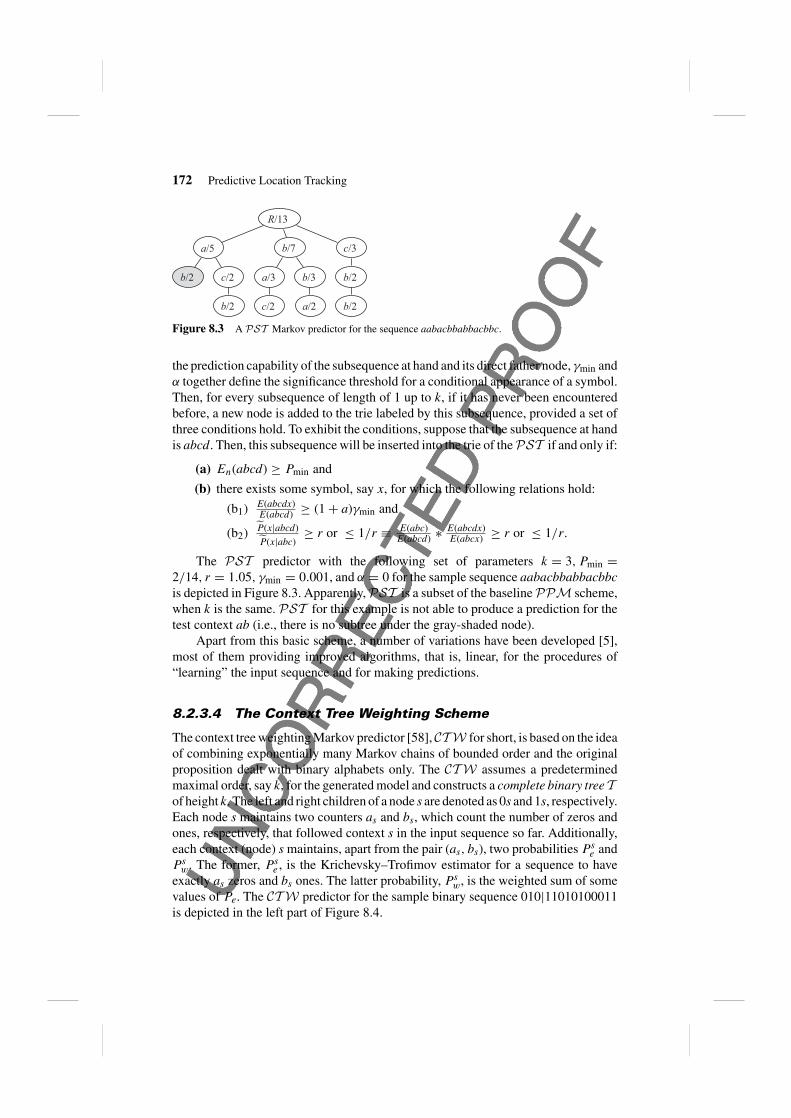
the prediction capability of the subsequence at hand and its direct father node, γmin andα together define the significance threshold for a conditional appearance of a symbol.Then, for every subsequence of length of 1 up to k, if it has never been encounteredbefore, a new node is added to the trie labeled by this subsequence, provided a set ofthree conditions hold. To exhibit the conditions, suppose that the subsequence at handis abcd. Then, this subsequence will be inserted into the trie of thePST if and only if:
(a) En(abcd) ≥ Pmin and
(b) there exists some symbol, say x, for which the following relations hold:
(b1) E(abcdx)E(abcd) ≥ (1 + a)γmin and
(b2) P(x|abcd)P(x|abc)
≥ r or ≤ 1/r ≡ E(abc)E(abcd) ∗ E(abcdx)
E(abcx) ≥ r or ≤ 1/r.
The PST predictor with the following set of parameters k = 3, Pmin =2/14, r = 1.05, γmin = 0.001, and α = 0 for the sample sequence aabacbbabbacbbc
is depicted in Figure 8.3. Apparently, PST is a subset of the baseline PPM scheme,when k is the same. PST for this example is not able to produce a prediction for thetest context ab (i.e., there is no subtree under the gray-shaded node).
Apart from this basic scheme, a number of variations have been developed [5],most of them providing improved algorithms, that is, linear, for the procedures of“learning” the input sequence and for making predictions.
8.2.3.4 The Context Tree Weighting Scheme
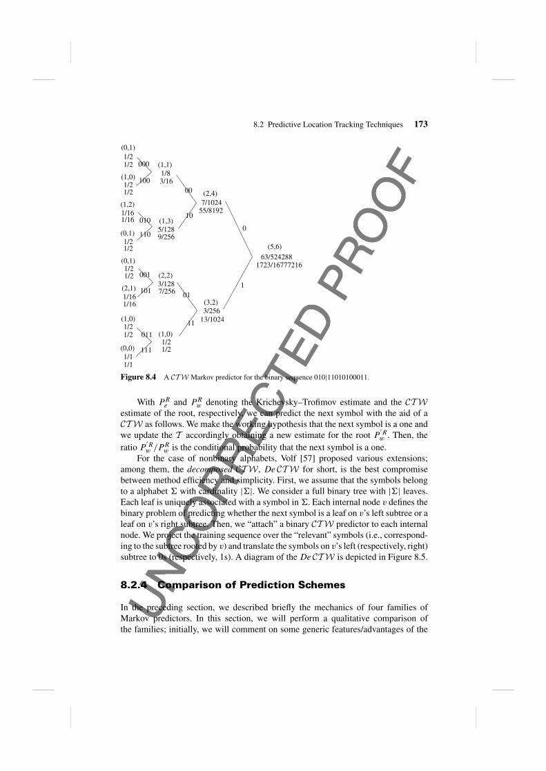
The context tree weighting Markov predictor [58],CT W for short, is based on the ideaof combining exponentially many Markov chains of bounded order and the originalproposition dealt with binary alphabets only. The CT W assumes a predeterminedmaximal order, say k, for the generated model and constructs a complete binary tree Tof height k. The left and right children of a node s are denoted as 0s and 1s, respectively.Each node s maintains two counters as and bs, which count the number of zeros andones, respectively, that followed context s in the input sequence so far. Additionally,each context (node) s maintains, apart from the pair (as, bs), two probabilities Ps
e andPs
w. The former, Pse , is the Krichevsky–Trofimov estimator for a sequence to have
exactly as zeros and bs ones. The latter probability, Psw, is the weighted sum of some
values of Pe. The CT W predictor for the sample binary sequence 010|11010100011is depicted in the left part of Figure 8.4.
8.2 Predictive Location Tracking Techniques 173
(0,0)1/11/1
1/21/2
1/161/16
(0,1)1/21/2
(1,0)
(2,1)
(0,1)1/21/2
1/16
(1,2)1/16
(0,1)1/21/2
1/21/2
(1,0)
(1,3)
(1,1)
(2,2)
(1,0)1/21/2
1/8
5/128
3/128
3/16
9/256
7/256
(2,4)7/1024
55/8192
(3,2)3/256
13/1024
63/524288
(5,6)
1723/16777216
0
000
111
11
00100
10010
110
011
001
011
101
Figure 8.4 A CT W Markov predictor for the binary sequence 010|11010100011.
With PRe and PR
w denoting the Krichevsky–Trofimov estimate and the CT Westimate of the root, respectively, we can predict the next symbol with the aid of aCT W as follows. We make the working hypothesis that the next symbol is a one andwe update the T accordingly obtaining a new estimate for the root P
′Rw . Then, the
ratio P′Rw /PR
w is the conditional probability that the next symbol is a one.For the case of nonbinary alphabets, Volf [57] proposed various extensions;
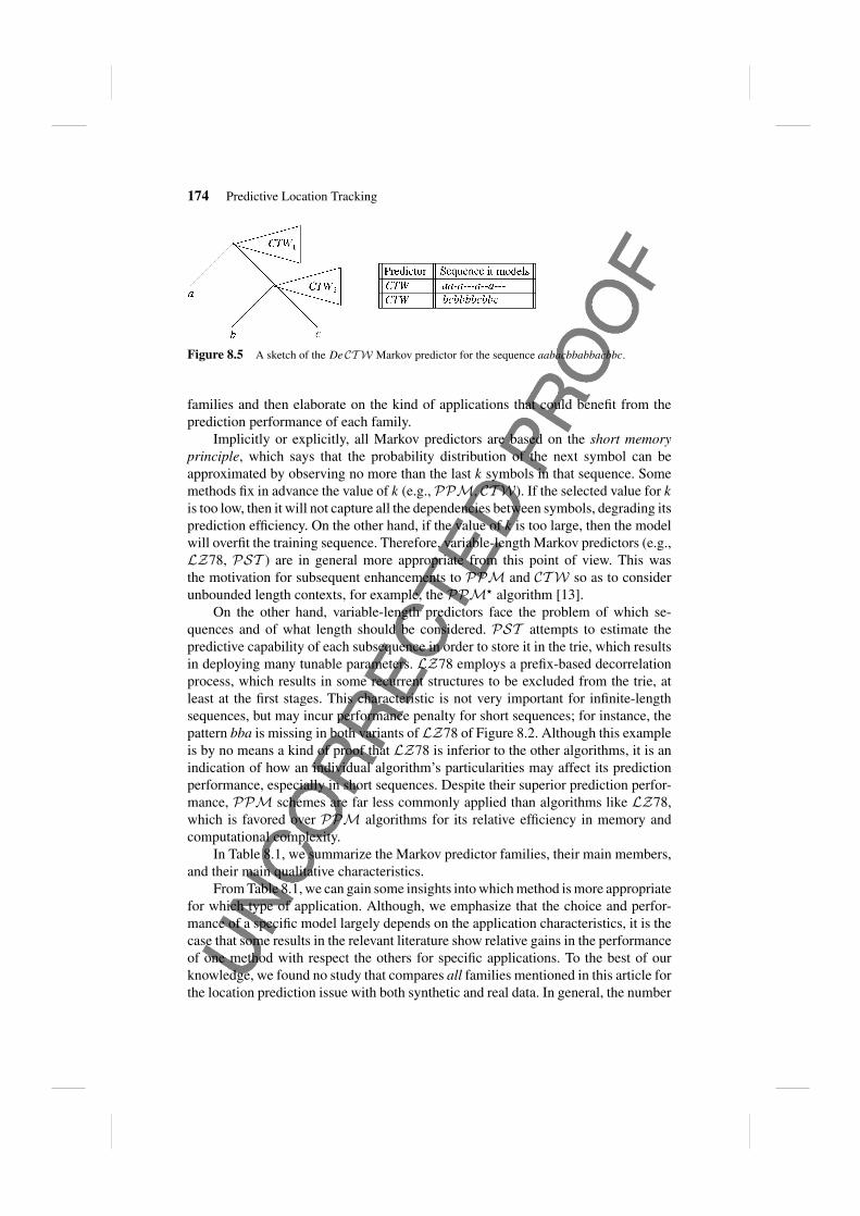
among them, the decomposed CT W , De CT W for short, is the best compromisebetween method efficiency and simplicity. First, we assume that the symbols belongto a alphabet � with cardinality |�|. We consider a full binary tree with |�| leaves.Each leaf is uniquely associated with a symbol in �. Each internal node v defines thebinary problem of predicting whether the next symbol is a leaf on v’s left subtree or aleaf on v’s right subtree. Then, we “attach” a binary CT W predictor to each internalnode. We project the training sequence over the “relevant” symbols (i.e., correspond-ing to the subtree rooted by v) and translate the symbols on v’s left (respectively, right)subtree to 0s (respectively, 1s). A diagram of the De CT W is depicted in Figure 8.5.
8.2.4 Comparison of Prediction Schemes
In the preceding section, we described briefly the mechanics of four families ofMarkov predictors. In this section, we will perform a qualitative comparison ofthe families; initially, we will comment on some generic features/advantages of the
174 Predictive Location Tracking
Figure 8.5 A sketch of the De CT W Markov predictor for the sequence aabacbbabbacbbc.
families and then elaborate on the kind of applications that could benefit from theprediction performance of each family.
Implicitly or explicitly, all Markov predictors are based on the short memoryprinciple, which says that the probability distribution of the next symbol can beapproximated by observing no more than the last k symbols in that sequence. Somemethods fix in advance the value of k (e.g., PPM, CT W). If the selected value for k
is too low, then it will not capture all the dependencies between symbols, degrading itsprediction efficiency. On the other hand, if the value of k is too large, then the modelwill overfit the training sequence. Therefore, variable-length Markov predictors (e.g.,LZ78, PST ) are in general more appropriate from this point of view. This wasthe motivation for subsequent enhancements to PPM and CT W so as to considerunbounded length contexts, for example, the PPM� algorithm [13].
On the other hand, variable-length predictors face the problem of which se-quences and of what length should be considered. PST attempts to estimate thepredictive capability of each subsequence in order to store it in the trie, which resultsin deploying many tunable parameters. LZ78 employs a prefix-based decorrelationprocess, which results in some recurrent structures to be excluded from the trie, atleast at the first stages. This characteristic is not very important for infinite-lengthsequences, but may incur performance penalty for short sequences; for instance, thepattern bba is missing in both variants of LZ78 of Figure 8.2. Although this exampleis by no means a kind of proof that LZ78 is inferior to the other algorithms, it is anindication of how an individual algorithm’s particularities may affect its predictionperformance, especially in short sequences. Despite their superior prediction perfor-mance, PPM schemes are far less commonly applied than algorithms like LZ78,which is favored over PPM algorithms for its relative efficiency in memory andcomputational complexity.
In Table 8.1, we summarize the Markov predictor families, their main members,and their main qualitative characteristics.
From Table 8.1, we can gain some insights into which method is more appropriatefor which type of application. Although, we emphasize that the choice and perfor-mance of a specific model largely depends on the application characteristics, it is thecase that some results in the relevant literature show relative gains in the performanceof one method with respect the others for specific applications. To the best of ourknowledge, we found no study that compares all families mentioned in this article forthe location prediction issue with both synthetic and real data. In general, the number

8.2 Predictive Location Tracking Techniques 175
Table 8.1 Qualitative Comparison of Discrete Sequence Prediction Models
Prediction method Overheads
Family Variant Markov class Train Parame/tion Storage Particularity
LZ78 [8] Variable Online Moderate Moderate May miss patterns[64] Variable Online Moderate Moderate
PPM [10] Fixed Offline Heavy Large Fixed length[14] Fixed Online Moderate Large High complexity[16] Fixed Offline Heavy Large
PST [5] Variable Offline Heavy Low Parameterization[41] Variable Offline Heavy Low
CT W [57] Fixed Online Moderate Large Binary nature[58] Fixed Online Moderate Large
of such studies is limited and the real data they use (when they use such) come fromlimited settings (e.g., university campuses) and not from users of commercial wirelesssystems, for example, cellular networks. Thus, it is not possible to draw safe conclu-sions from these works. Worthwhile studies containing comprehensive experimentswith real data are reported in Refs. [11, 21, 37, 45].
Although alternative approaches could be possible, we prefer to present oursuggestions for policy selection along two primary dimensions; the first dimensionreflects the type of the problem (i.e., location prediction) and the second dimensionreflects the “network part,” where the prediction is carried out (i.e., fixed, resource-richnetwork servers, or resource-starving mobile hosts).
For mobile applications, some very important intuitive results, which have alsobeen confirmed experimentally [25], can be stated: (a) user interests vary significantlywith time (not “strong” stationarity), (b) many alternative paths exist that lead to thesame target location, thus the regularity patterns are “blurred” by noise. Due to thefirst observation, the possibility of using LZ78 types of predictors is rather small.Due to the variance in the length of the individual client’s trajectories, the rest ofthe variable-order Markov predictors are more appropriate; PST would be a perfectchoice under the assumptions that the procedure is performed offline and it runs on aresource-rich server, or a relatively powerful laptop.
If energy conservation is the main issue in these applications (small portabledevices like PDAs, mobile phones), then the choice of PPM style predictors seemsmore appropriate since they are online, but they sacrifice some prediction performance(due to the relatively small and fixed order model employed) for reduced modelcomplexity. The second observation may turn all prediction methods inefficient, sinceit violates the “consecutiveness” property of appearance of the symbols in the patterns,upon which property all described Markov predictors rely. In cases where “noisesymbols” are interleaved in pattern subsequences, the modified Markov predictorsdescribed in Refs. [16, 37] can be employed, but these algorithms are offline and
176 Predictive Location Tracking
require substantial resources (memory, power) to be executed. Therefore, they couldonly be used by fixed network servers, which collect huge amounts of user trajec-tories.
Location prediction is considered a relatively manageable problem, because of thefew alternatives in possible contexts (i.e., hexagonal architecture of cellular systems,few fixed access points in wireless LANs, and smart home applications) and becauseof the “strong” stationarity (i.e., few habitual routes in campuses/cities, few travelpaths in urban regions—road network).
For location, prediction applications, several families of Markov predictors couldbe used in some specific scenarios each. For dynamic tracking of mobile hosts (withthe tracking application running either in the network server or the mobile host),PPM and LZ78 methods are appropriate. The small order PPM model and theenhanced LZ78 [8] are expected to achieve the best performance, because of theundoubted validity of the stationarity assumption. Indeed, the study in Ref. [45]confirmed that intuitive results. These variants are perfect fit for dynamic resourceallocation before handovers, as well. For location area design applications, wherewe are interested in discovering “long-standing” repetitive user routes, the process isoffline and therefore methods likePST or [16, 37] are appropriate and less vulnerableto statistical deviation.
8.3 PREDICTIVE LOCATION INDEXING TECHNIQUES
In the previous section, we presented the dominant approaches for predictive locationtracking for the case of a symbolic topology model. In many cases though, we areinterested in tracking the location of mobiles at a finer granularity of space and time.Consider, for instance, our interest in tracking the trajectories of birds, airplanes, orsatellites, which are considered as points, or our interest in tracking the movement ofa tropical storm, of fires. This interests stems from our need to answer queries like,“When two satellites are going to meet?”, “Is the fire threatening village Thetidio?”,and so on.
This leads to the idea of storing in a database for each moving object not thecurrent position but rather a motion vector, which amounts to describing the positionas a function of time. That is, if we record for an object its position at time t0 togetherwith its speed and direction at that time, we can derive expected positions for all timesafter t0. Of course, motion vectors also need to be updated from time to time, but muchless frequently than positions. Hence, from the location management perspective, weare interested in maintaining dynamically the locations of a set of currently movingobjects and in being able to ask queries about the current positions, the positions inthe near future, or any relationships that may develop between the moving entitiesand static geometries over time.
To support such functionality, the database must build indexes; the main task ifan index is to ensure fast access to single or several records in the database on thebasis of a search key and thus avoid an otherwise necessary naive scan. Numerousindexes able to support continuous movement have appeared in the literature [18].
8.3 Predictive Location Indexing Techniques 177
The indexes capable of accommodating moving objects can be generally categorizedinto those optimizing queries about past states of movement and those tailored toserving queries about future positions of the moving objects; the first type of queriesare called historical, while the second one are termed predictive. In the following, wewill address the predictive location indexing techniques.
8.3.1 Assumptions and Terminology
In the majority of the applications, the size and the shape of the moving objectsare insignificant. Consequently, every object is modeled as a geometric point whoseposition consists of a time function x(t) of the particular motion parameters. On thebasis of x(t), the applications evaluate the future object locations. Furthermore, it isexpected that the involved objects have the capacity and the obligation of periodicallyreporting any alteration occurring in x parameters. As an example, in most cases, x(t) isa linear function of time x(t) = x(tref ) + v(t − tref ), where the two parameters are theposition x(tref ) at the reference time tref and the velocity vector v. Generally speaking,the equation parameters specify a dual to the time–location space framework.
As far as the type of queries is concerned, they can be classified as range queriesand proximity or nearest neighbor (NN) ones. A range query is termed (i) time-sliceor snapshot (r, t) when, given a region r, usually a hyper-rectangle, located at timet, it asks for all moving objects contained in r at that time; (ii) window (r, [t1, t2])when it asks for all objects crossing a hyper-rectangle r during a time interval [t1, t2];(iii) moving (r1, r2, [t1, t2]) when it inquires all objects crossing the trapezoid formedby connecting the hyper-rectangle r1 at time t1 and the hyper-rectangle r2 at time t2;and (iv) selectivity or aggregate (r, [t1, t2]) when, given a region r and a time interval[t1, t2], it requests an estimation about the number of the objects that will pass throughr during [t1, t2]. Types (i)–(iii) are also known as range reporting, whereas type (iv)is well tailored to the case of limited memory and strict real-time processing demand.
On the other hand, a proximity query inquires for the k nearest moving objectsto a given location at a time instance t or during a time interval [t1, t2], with k ≥ 1.Sometimes, all objects having a given location as their nearest neighbor are asked for;this kind of searching is termed reversed nearest neighbor searching (RNN).
In the above definitions, two variations are possible: First, the query range/pointalso moves which makes the query continuous. And second, the answer set may bereturned with temporal or spatial validity information, informing thus the user aboutthe future time t the result expires or the validity region r containing the query positionwithin which the answer remains valid.
Concluding this subsection, we briefly discuss the R-tree [19], a general purposepractical indexing structure, since the majority of the solutions to be presented are builtupon it. So, an R-tree is a height-balanced tree that can be considered as an extensionof the B+-tree for multidimensional data. The minimum bounding rectangle (MBR)of each geometric object, along with a pointer to the disk address where the objectactually resides, are stored into the leaves. Each internal node entry consists of a pair(pointer to a subtree T , MBR of T ), with the MBR of a tree T defined as the MBR
178 Predictive Location Tracking
S
T
BA C GD HEF
P RQ
C
B
G
EA
H
F
Q
PR
D
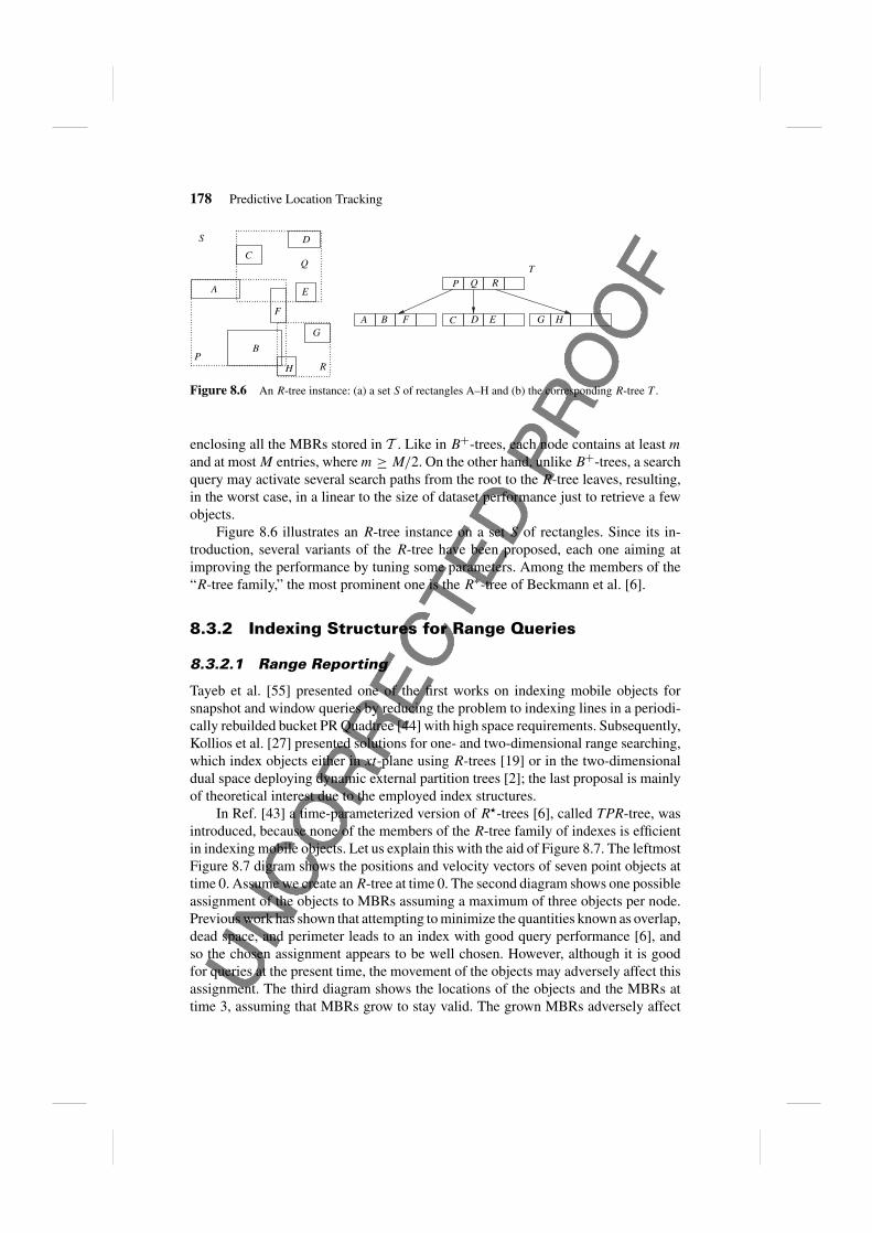
Figure 8.6 An R-tree instance: (a) a set S of rectangles A–H and (b) the corresponding R-tree T .
enclosing all the MBRs stored in T . Like in B+-trees, each node contains at least m
and at most M entries, where m ≥ M/2. On the other hand, unlike B+-trees, a searchquery may activate several search paths from the root to the R-tree leaves, resulting,in the worst case, in a linear to the size of dataset performance just to retrieve a fewobjects.
Figure 8.6 illustrates an R-tree instance on a set S of rectangles. Since its in-troduction, several variants of the R-tree have been proposed, each one aiming atimproving the performance by tuning some parameters. Among the members of the“R-tree family,” the most prominent one is the R∗-tree of Beckmann et al. [6].
8.3.2 Indexing Structures for Range Queries
8.3.2.1 Range Reporting
Tayeb et al. [55] presented one of the first works on indexing mobile objects forsnapshot and window queries by reducing the problem to indexing lines in a periodi-cally rebuilded bucket PR Quadtree [44] with high space requirements. Subsequently,Kollios et al. [27] presented solutions for one- and two-dimensional range searching,which index objects either in xt-plane using R-trees [19] or in the two-dimensionaldual space deploying dynamic external partition trees [2]; the last proposal is mainlyof theoretical interest due to the employed index structures.
In Ref. [43] a time-parameterized version of R�-trees [6], called TPR-tree, wasintroduced, because none of the members of the R-tree family of indexes is efficientin indexing mobile objects. Let us explain this with the aid of Figure 8.7. The leftmostFigure 8.7 digram shows the positions and velocity vectors of seven point objects attime 0. Assume we create an R-tree at time 0. The second diagram shows one possibleassignment of the objects to MBRs assuming a maximum of three objects per node.Previous work has shown that attempting to minimize the quantities known as overlap,dead space, and perimeter leads to an index with good query performance [6], andso the chosen assignment appears to be well chosen. However, although it is goodfor queries at the present time, the movement of the objects may adversely affect thisassignment. The third diagram shows the locations of the objects and the MBRs attime 3, assuming that MBRs grow to stay valid. The grown MBRs adversely affect
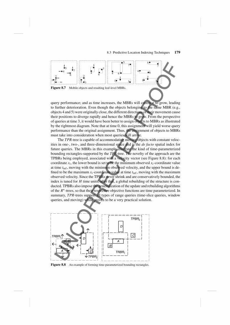
8.3 Predictive Location Indexing Techniques 179
6
1 1 1 1
2 22 2
3 3 3 3
4 4 44
55
5 5
77
7 7
6 6 6
Figure 8.7 Mobile objects and resulting leaf-level MBRs.
query performance; and as time increases, the MBRs will continue to grow, leadingto further deterioration. Even though the objects belonging to the same MBR (e.g.,objects 4 and 5) were originally close, the different directions of their movement causetheir positions to diverge rapidly and hence the MBRs to grow. From the perspectiveof queries at time 3, it would have been better to assign objects to MBRs as illustratedby the rightmost diagram. Note that at time 0, this assignment will yield worse queryperformance than the original assignment. Thus, the assignment of objects to MBRsmust take into consideration when most queries will arrive.
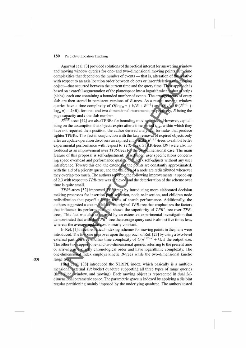
The TPR-tree is capable of accommodating moving objects with constant veloc-ities in one-, two-, and three-dimensional space and is the de facto spatial index forfuture queries. The MBRs in this example illustrate the kind of time-parameterizedbounding rectangles-supported by the TPR-tree. The novelty of the approach are theTPBRs being employed, associated with a velocity vector (see Figure 8.8): for eachcoordinate xi, the lower bound is set to be the minimum observed xi-coordinate valueat time tref , moving with the minimum observed velocity, and the upper bound is de-fined to be the maximum xi-coordinate value at time tref , moving with the maximumobserved velocity. Since the TPBRs never shrink and are conservatively bounded, theindex is tuned for H time units; after that, a global rebuilding of the structure is con-ducted. TPBRs also impose the generalization of the update and rebuilding algorithmsof the R∗-trees, so that their respective objective functions are time parameterized. Insummary, TPR-trees support all types of range queries (time-slice queries, windowqueries, and moving) while proven to be a very practical solution.
B
A
B
A
C
DC
D
TRBR1
TPBR2
TRBR1
TPBR2
Figure 8.8 An example of forming time-parameterized bounding rectangles.
180 Predictive Location Tracking
Agarwal et al. [3] provided solutions of theoretical interest for answering windowand moving window queries for one- and two-dimensional moving points with timecomplexities that depend on the number of events — that is, alteration of the relativewith respect to an axis location order between objects or insert/deletion of a movingobject—that occurred between the current time and the query time. Their approach isbased on a careful segmentation of the plane/space into a logarithmic number of strips(slabs), each one containing a bounded number of events. The arrangements of everyslab are then stored in persistent versions of B-trees. As a result, moving windowqueries have a time complexity of O(logB n + k/B + Bi−1) and O(
√n/Bi(Bi−1 +
logB n) + k/B), for one- and two-dimensional movements, respectively, B being thepage capacity and i the slab number.
REXP-trees [42] use also TPBRs for bounding moving objects. However, capital-izing on the assumption that objects expire after a time period texp, within which theyhave not reported their position, the author derived analytical formulas that producetighter TPBRs. This fact in conjunction with the lazy removal of expired objects onlyafter an update operation discovers an expired entry make REXP-trees to exhibit betterexperimental performance with respect to TPR-trees. STAR-trees [39] were also in-troduced as an improvement over TPR-trees for the two-dimensional case. The mainfeature of this proposal is self-adjustment: based upon user specifications concern-ing space overhead and performance quality, the index self-adjusts without any userinterference. Toward this end, the extends of the points are constantly approximated,with the aid of a priority queue, and the children of a node are redistributed wheneverthey overlap too much. The authors reported the following improvements: a speed-upof 2.3 with respect to TPR-tree was achieved and the deterioration of the scheme overtime is quite small.
TPR∗-trees [52] improved TPR-trees by introducing more elaborated decisionmaking processes for insertion path selection, node re-insertion, and children noderedistribution that payoff a lot in terms of search performance. Additionally, theauthors suggested a cost model for the original TPR-tree that emphasizes the factorsthat influence its performance and shows the superiority of TPR∗-tree over TPR-trees. This fact was also confirmed by an extensive experimental investigation thatdemonstrated that with the TPR∗-tree the average query cost is almost five times less,whereas the average update cost is nearly constant.
In Ref. [1] three theoretical indexing schemes for moving points in the plane wereintroduced. The first one improves upon the approach of Ref. [27] by using a two-levelexternal partition tree and has time complexity of O(n1/2+ε + k), k the output size.The other two support one- and two-dimensional queries referring to the present timeor arriving in a strictly chronological order and have logarithmic complexity. Theone-dimensional index employs kinetic B-trees while the two-dimensional kineticrange trees.[Q3]
Patel et al. [38] introduced the STRIPE index, which basically is a multidi-mensional external PR bucket quadtree supporting all three types of range queries(time slice, window, and moving). Each moving object is represented in dual 2d-dimensional parametric space. The parametric space is indexed by applying a disjointregular partitioning mainly imposed by the underlying quadtree. The authors tested
8.3 Predictive Location Indexing Techniques 181
the performance of STRIPE against the TPR∗-tree thoroughly and found that theirproposal is faster in both update and query time; namely, queries are faster by a fac-tor of four, while the update operations complete by an order of magnitude quickersince TPR*-trees have the disadvantages of poor cache locality and multiple pathtraversals.
Tao et al. [48] coped with the case of circular static range query during a timeinterval for moving objects with unknown moving patterns. In order to support arbi-trarily movements, Tao et al. suggested a monitor-and-index framework: Each movingobject individually and constantly computes the recursive function that best describesits movement using motion matrices introduced by the authors. On the other hand,the server adopts the same coarse polynomial function m for every object. The latterfact introduces imprecision that is dealt with a two-step process. During the filteringphase, all objects that either definitely or possibly satisfy the query are determinedusing STP-tree. STP-tree can be considered as a generalization of both TPR andTPR∗-trees to arbitrary polynomial functions m. In a second refinement step, theserver communicates with the doubtful objects that evaluate the query according totheir own accurate moving function and send back the result if necessary along withthe corrected parameters of m. The applicability of the proposal is thoroughly investi-gated through a series of experiments that concern both the movement approximationmethod and the new index.
8.3.2.2 Range Aggregate.
In 2002, Choi and Chung [12] presented the first work on rectangular range selectivityfor static queries. Their solution for the one-dimensional case is based on the simpleobservation that a point satisfies the query range r if and only if the segment formed byits (tentative) position at the start and the end of the query time interval intersects r. Theauthors proposed a histogram-based counting solution so that the spatial universe ispartitioned into a number of time-evolving buckets. This method was also extended tothe two-dimensional case by projecting objects and queries on each spatial dimensionand evaluating the selectivity as the product of the one-dimensional results.
The previous method suffers from overestimated results since the projectionoverlooks necessary temporal conditions. Tao et al. [54] achieved better estimationresults by dropping the projection step; their solution tackles directly the problem withthe deployment of a spatio-temporal histogram, which considers both locations andvelocities. The authors report significant improvements in selectivity precision andmanipulation of updates. In Ref. [20], one- and two-dimensional movements werealso coped with. As a matter of fact, two solutions were introduced: One is also basedon multidimensional histograms, which, none the less, are defined on dual space. Theaccommodation of the moving objects into an index is prerequisite for the secondsolution. Namely, the summaries of each leaf entry, in the form of number of objectsand their bounded rectangular spatial extent, are stored in a hash table that is used foroutput extrapolation.
In contrast to the previous three solutions, in Ref. [53] random sampling waschosen for selectivity estimation in order to spare space and processing overhead.
182 Predictive Location Tracking
Particularly, the introduced method of Venn sampling employs a set S of m pivotqueries, which represent the actual distribution and are perfectly estimated. The mostinteresting part is that, based on S, a weighted sample of m moving objects, non-necessarily belonging to the underlying dataset, is formed and communicated to themoving objects. This sample is queried against any incoming query and the sum ofweights of qualifying objects is returned to the user. The system constantly monitorsthe quality of the sample set in collaboration with the moving objects; in case the es-timation error surpluses a threshold, the sample weights but not the respective sampleobjects are adjusted. The authors present experimental results, rendering the proposalquite appealing.
8.3.3 Indexing Structures for Nearest NeighborQueries
Kollios et al. [26] introduced practical yet preliminary solutions for locating thenearest moving neighbor of a static query in the plane permitting object movementin fixed line segments either arbitrary or restricted. They consider both the cases ofindexing in the xt-plane and in the dual plane. The first case allows indexing withstandard spatial indexes, like, for example, R-trees [19], while the second one utilizesB+-trees [15] and dual plane segmentation in horizontal stripes.
Song and Roussopoulos [46] studied the continuous kNN problem, which in-quires for the k-nearest static neighbors of a moving query point. Their approach isbased on the observation that as the query point is moving to new locations, somepreviously reported neighbors are still among the k closest ones. This fact is formallyexpressed by a series of conditions that allow the employment of standard indexingstructures like R-trees.
Zheng and Lee [63] considered enhancing NN queries with validity information.The approach is quite simple: The nearest neighbor of a moving point is calculatedusing the Voronoi diagram of the static dataset. Since the Voronoi cell c of the nearestneighbor is available, the maximum circle around the query point that does not crossany boundary edge of c consists a safe lower bound for the validity of the query result.
In Ref. [7], two-dimensional nearest neighbor and reverse nearest neighborqueries for a query point q during a time interval t were treated by properly ex-tending TPR-tree algorithms. NN queries apply a depth-first search technique thatconstantly prunes TPBRs with no chance enclosing closest points. The RNN queriesare more elaborate: the space around the query point q is divided into six equal sectorssi by straight lines intersected at q, since there must exist at most six RNN points, atmost one in each si. Therefore, sectors containing two or more nearest points of q arediscarded and the search is restricted among the nearest neighbors of the rest.
Continuous NN queries for static datasets were also treated, albeit from a differentperspective, in Ref.[22]. This solution is built upon ellipsoid areas around the movingquery point that are generated utilizing current, past, and future trajectory positionsand carefully selected metrics. The static dataset, on the other hand, is indexed witha “spatial” structure, like, for example, R-trees. Since the previous answers are not

8.3 Predictive Location Indexing Techniques 183
reused as the query point changes position, this method needs involved tuning to beeffective.
Tao et al. [51] considered continuous kNN search when the static input dataset isaccommodated in an R-tree T and the query point is linearly moving. When k = 1,these assumptions guarantee that the output set consists of a sequence of points pi,which partition the movement line segment into a sequence of disjoint segments si.Every point in si has pi as its nearest neighbor. These facts suggest a branch-and-bound investigation of T employing heuristic node pruning. Tao et al. also generalizedthe pruning rules for the continuous kNN case, providing an extensive experimentalevaluation of their proposal.
Aggarwal and Agrawal [4] introduced NN solutions for objects moving in non-linear trajectories of arbitrary dimensionality whose parametric representation satisfythe so-called convex hull property. The d-dimensional trajectories with constant ve-locity, d-dimensional parabolic trajectories, elliptic orbits, and trajectories that acceptapproximate Tailor expansion belong to this category. Due to the convex hull property,the locality in parametric space corresponds to the locality in the positions of objects,and, thus NN search can be accomplished by a branch-and-bound, best-first algo-rithm conducted in a classical spatial index. The authors demonstrated their methodfor linear and parabolic trajectories in three- and two-dimensional space, respectively.
TPR-trees algorithms were enhanced in Ref. [40], so that continuous kNN querieson moving points during a time interval [t1, t2] can be served. The suggested solutioncapitalizes on the following geometric fact: the kNN points can be determined by thek levels of the arrangement of the squared distance functions of the moving pointswith respect to the moving query during [t1, t2]. Therefore, after collecting at least k
points by a depth-first traversal of the underlining TPR-tree according to the minimumsquared distance metric between the moving query and the bounding rectangles at t1,the kNN points of [t1, t2] are determined. Then, in a second stage, the TPR-tree isonce more traversed, in order to refine and finalize the output set.
Iwerks et al. [23] also presented algorithms for answering continuous kNNqueries on a constantly moving point set with respect to either a static or a mov-ing query point. Their approach runs also in two phases. During first phase, input setis filtered with a continuous query that asks about objects within a distance bound d.Then, the qualified points are ranked with a priority queue, which tracks the timeinstances when points change their distance to the query point or when points changetheir order with respect to a current kNN point.
Nearest neighbor queries, among others, were also treated in Ref. [1]. Specifi-cally, Agarwal et al. suggested an algorithm that offers approximate results to NNsearching by replacing the Euclidean metric with a polyhedral one. The input set isaccommodated into a three-level composite index of O(n1/2+ε/
√δ) time complexity,
0 < δ, ε < 1. The first two levels are external partition trees on dual space. The lastlevel stores the lower envelope of the trajectories in linear lists.
The conceptual partitioning method (CPM) was introduced in Ref. [35] for con-stantly monitoring of multiple continuous NN queries in highly dynamic environ-ments. In brief, the space is partitioned by a regular grid and indexed in main memory.Every cell of this grid maintains the list of objects residing therein and every posed

184 Predictive Location Tracking
query along with its current result set is stored in a table. Additionally, CPM imposesa total order on the cells around every query based on proximity criterion. In that way,every update in both the data and the query set is tackled with minimal computationalcosts without any assumptions about the occurring moving patterns; this is depictedby both qualitative and thorough experimental analysis.
After the previous work, Mouratidis et al. [36] presented a main memory solutionfor incremental monitoring of continuous kNN queries when the query and the data ob-jects move in road networks. Their approach basically is based on network expansionabout the query until k nearest neighbors are collected. The formed shortest path treeis stored along with the query so that any updates are smoothly incorporated. More-over, the authors proposed a method for computation sharing among queries whoseshortest paths are crossed. All suggested solutions are experimentally evaluated.
Finally, Lee et al. [30] treated continuous nearest surrounder (NS) queries thatask for the nearest neighbors at individual distinct angles from the query point. NSqueries, thus, monitor the nearest neighbors around the queries by considering boththe distance and the angular attributes. The system registers the objects’ locations inan R-tree and the queries, along with their current results, in a hash table so that anyupdate of either data or query objects can be incrementally evaluated, capitalizing onthe notion of “safe regions” firstly introduced in Ref. [29].
8.3.4 Indexing Structures for Both Windowand Nearest Neighbor Queries
In Ref. [50] time-parameterized window and kNN queries (TP) were introducedwhich, along with the objects that satisfy the spatial conditions, also return the expi-ration time of the validity of the answer and the change that invalidates the answer atthat time. The key concept of this approach is the influence time that is associated withevery moving object o and indicates the time o influences the validity of the answer.By definition, the expiration time of the answer equals the minimum influence time ofall objects which, in turn, can be evaluated with a NN search where the distance metricis the influence time. This observation is valid for both window and kNN queries. Theauthors proved analytical formulas for evaluating the influence times of an object. Asa result, standard branch-and-bound traversal of the index accommodating the objectset can be employed. Their solution also treats continuous spatio-temporal queries byposing a TP query every time the current result expires. Finally, TP queries can alsoserve earliest event queries that ask for the earliest time in the future a certain eventcould take place; for example, one may need to figure out the first time a moving querypoint q meets another moving object. By surrounding q with a time-varying radiuscycle, this query reduces to TP by evaluating the earliest time the circle contains apoint, which, in turn, equals to determining the smallest radius of such a circle.
Building upon Ref. [50], Zhang et al. [61] dealt also with validity kNN andwindow queries. In the first case, order-k Voronoi cells comprise the validity regions.These can be found implicitly by, first, generating the nearest neighbors and thenissuing time-parameterized kNN queries for locating points that define their border.
8.3 Predictive Location Indexing Techniques 185
In the second case, the maximal rectangle r around the center of the window, withinwhich the result remains unchanged, is first evaluated. Then, r is refined by subtractingthe parts that would force the query to mistakenly contain points not in the reportedanswer. These two steps involve one standard window query, one “holey” windowquery, and few main memory TP window queries.
Tao et al. [49] proved a number of theoretical bounds on validity range andNN queries. Specifically, when the query’s length and movement are chosen froma constant number of combinations and the point set is static, the query costis logarithmic and the space is linear. When the point set is static, the querylength is arbitrarily, and when the movement is axis-parallel, then the time com-plexity is O(log2
B(n/B)/ logB logB(n/B)) and the space cost is O(n/B logB(n/B)/logB logB(n/B)). On the other hand, in the case of static input point set and querieswith arbitrary length and movement, the space complexity is O(n/B) while the querycosts are O((n/B)1/2+ε). When the data points are dynamic and the query is static,the query has logarithmic complexity and space is bounded by O(n2/B logB(n/B)).The case of both dynamic data points and query point is only considered in one-dimensional space, proving a linear space and logarithmic time complexity. As faras the NN search query is concerned, when the input point set is static lying in theplane or comprised of moving points on the line, the solution is of linear space andlogarithmic query cost.
The Bx-trees were introduced in Ref. [24], which are capable of serving range,and kNN queries as well as their continuous counterparts. The main ingredient of thismethod is movement linearization: The time axis is partitioned into intervals of timeunits, and each interval is further subdivided into n subintervals of equal length. Everyobject, according to its tref , is assigned to one subinterval. Within each subinterval, thepositions of the objects fallen in are linearized according to a space filling curve andthen stored into a B+-tree. Therefore, the Bx-tree is actually a sequence of B+-treesevolving as time goes by. The authors conducted extensive experiments, which showthe superiority of Bx-trees over TPR-trees for all kinds of queries. Here we mustnote that BBx-trees [32] were introduced as a natural extension of Bx ones, able ofanswering both predictive and historical queries.
After observing that the linearization process of Ref. [24], in Ref. [59] onlyobject’s locations were considered, leading thus to excessive false hits, proposedBdual-trees. Bdual-trees also deploy B+-trees indexing, none the less, a space-fillingcurve that is based on both object locations and velocities. The authors demonstratedthe superiority of their method over Bx-trees both analytically (i.e., using derivedformulas) and experimentally—the experimental study also gives data for STRIPESand TPR∗-trees. In a nutshell, Bdual-trees can be considered as the state-of-the-artsolution in its category.
8.3.5 Evaluation of Predictive Indexing
In overall, TPR-trees [43] and its descendant variations, like TPR∗-trees [52], canbe considered the most appropriate and practical choice for serving range queries.

186 Predictive Location Tracking
In case of limited resources, the Venn sampling technique of Ref. [53] is deemed anatural option. As far as nearest neighbor queries is concerned, the TPR-tree variationof Ref. [40] and the CPM of Ref. [35] are both competent candidates. Finally, Bx-trees [24] and Bdual-trees [59] proved to be apt solutions when one wants to treatequally well range and nearest neighbor queries.
Regarding future steps toward developing more indexing mobiles, it would be[Q2]
very helpful the indexes to provide results that capture the uncertainty associated withthe location of moving objects due to network delays and the continuous character ofmotion. It would be also very interesting to efficiently cope with nonlinear trajecto-ries since the scope and the range of indexable moving objects will be significantlyextended. Another appealing subject, especially for extending mobile applicationcapabilities, is the design of indexing structures capable of serving mixed queriesconcerning the past and the future of movement The incremental valuation of va-lidity queries is very intriguing, as well. Finally, from an engineering perspective,it would be very helpful (i) to test all indexes with real datasets, as, until now, ev-ery experimental investigation is conducted with semireal ones, where the movementcomponent is actually generated; and (ii) to design efficient updating algorithms forthe indexes, different from the usual “deletion and re-insertion” practice, acceptingperhaps a tradeoff between either the query time or the accuracy of the result and theupdate time.
8.4 CONCLUSION
This chapter identified the inherent uncertainty in the movement of mobiles in areascovered by wireless networks and the problems caused to resource allocation due tothis uncertainty. Starting from this fundamental observation, it subsequently recog-nized the benefits of being able to forecast the future locations of the mobile hosts.This ability could be used to act proactively, instead of reactively, to many situa-tions. For instance, having estimates of future positions of mobile hosts, the networkcould take appropriate decisions regarding the bandwidth that will allocate to the cellscontaining these locations. In addition, in wireless ad hoc networks, where commu-nication between nodes is performed on a store-and-forward basis for nodes not inclose proximity, the communication could be deferred until the nodes come closer toeach other, thus saving network resources, like precious bandwidth and storage spacein the intermediate nodes, reducing packet collisions, and so on.
However, predictive location tracking can be performed only if the mobiles’movements exhibit some degree of regularity, thus making the construction of mo-bility models feasible. The generic principle governing location prediction can besummarized in a short sentence: study the present and project to the future. Exploit-ing this principle, the issue of location prediction turned out to be a matter of recordingthe present mobile trajectories and developing mobility models from these. The stor-age of the trajectories should be of the kind to allow compact representation and atthe same time efficient generation of predictions.
References 187
Subsequently, we investigated two different scenarios for predictive location pre-diction. According to the first scenario, the roaming area of the mobiles can be con-sidered as a union of nonoverlapping cells of arbitrary geometry and according to thesecond scenario, the location tracking is performed at the granularity of geographicalcoordinates. For the first scenario, we modeled the problem of predictive locationtracking in terms of the discrete sequence prediction problem. For this latter problem,we presented Markov predictors as a practical and high-performance solution, cate-gorized them into four families giving their qualitative characteristics, their strengths,and their weaknesses. For the second scenario, which is more tightly coupled with lo-cation databases, we surveyed the state-of-the-art techniques for constructing indexescapable of answering queries that mainly concern various complex future predicates.
Undoubtedly, predictive location tracking is very important for reducing the la-tency and the resource consumption in any wireless network or for prolonging thelifetime of wireless ad hoc networks. However, the problem is not easily manageabledue to the difficulty of constructing models representing the actual mobile trajec-tories. Although very significant steps have been taken toward achieving this target,work is still needed to characterize the predictability of mobile trajectories, to analyzecollections of real mobile trajectories, to develop more effective prediction models,and mainly to develop distributed models of prediction through cooperation, whichwill be suitable for the emerged area of wireless sensor networks.
ACKNOWLEDGMENTS
Research supported by a ET grant in the context of the project “Data Manage-ment in Mobile Ad Hoc Networks” funded by �Y�AOPA� II national researchprogram.
REFERENCES
1. P. K. Agarwal, L. Arge, and F. Erickson. Indexing moving points. J. Comput. Syst. Sci., 66(1):207–243, 2003.
2. P. K. Agarwal, L. Arge, F. Erickson, P. G. Franciosa, and J. S. Vitter. Efficient searching with linearconstraints. J. Comput. Syst. Sci., 61(2):194–216, 2000.
3. P. K. Agarwal, L. Arge, and J. Vahrenhold. Time responsive external data structures for movingpoints. In Proceedings of the International Workshop on Distributed Algorithms and Data Structures(WADS), Vol. 2125, Lecture Notes in Computer Science, pp. 50–61, 2001.
4. C. C. Aggarwal and D. Agrawal. On nearest neighbor indexing of nonlinear trajectories. In Proceedingsof the ACM Symposium on Principles Of Database Systems (PODS), pp. 252–259, 2003.
5. A. Apostolico and G. Bejerano. Optimal amnesic probabilistic automata or how to learn and classifyproteins in linear time and space. J. Comput. Bio., 7(3–4):381–393, 2000.
6. N. Beckmann, H.-P. Kriegel, R. Schneider, and B. Seeger. The R∗-tree: an efficient and robust accessmethod for points and rectangles. In Proceedings of the ACM International Conference on Manage-ment of Data (SIGMOD), pp. 322–331, 1990.
7. R. Benetis, C. S. Jensen, G. Karciauskas, and S. Saltenis. Nearest neighbor and reverse nearestneighbor queries for moving objects. Very Large Data Bases J., 15(3):229–250, 2006.

188 Predictive Location Tracking
8. A. Bhattacharya and S. K. Das. LeZi-Update: an information-theoretic framework for personal mo-bility tracking in PCS networks. ACM/Kluwer Wireless Networks, 8(2–3):121–135, 2002.
9. S. Chakraborty, Y. Dong, D. K. Y. Yau, and J. C. S. Lui. On the effectiveness of movement prediction toreduce energy consumption in wireless communication. IEEE Trans. Mobile Comput., 5(2):157–169,2006.
10. X. Chen and X. Zhang. A popularity-based prediction model for Web prefetching. IEEE Comput.,36(3):63–70, 2003.
11. F. Chinchilla, M. Lindsey, and M. Papadopouli. Analysis of wireless information locality and as-sociation patterns in a campus. In Proceedings of the IEEE International Conference on ComputerCommunications (INFOCOM), Vol. 2, pp. 906–917, 2004.
12. Y.-J. Choi and C.-W. Chung. Selectivity estimation for spatio-temporal queries to moving objects. InProceedings of the ACM International Conference on Management of Data (SIGMOD), pp. 440–451,2002.
13. J. G. Cleary and W. J. Teahan. Unbounded length contexts for PPM. Comput. J., 40(2–3):67–75, 1997.14. J. G. Cleary and I. H. Witten. Data compression using adaptive coding and partial string matching.
IEEE Trans. Commun., 32(4):396–402, 1984.15. D. Comer. The ubiquitous B-tree. ACM Comput. Surv., 11(2):121–137, 1979.16. M. Deshpande and G. Karypis. Selective Markov models for predicting Web page accesses. ACM
Trans. Internet Technol., 4(2):163–184, 2004.17. M. Feder, N. Merhav, and M. Gutman. Universal prediction of individual sequences. IEEE Trans.
Inform. Theory, 38(4):1258–1270, 1992.18. R. H. Guting and M. Schneider. Moving Objects Databases. Series in Data Management Systems.
Morgan-Kaufmann, 2005.19. A. Guttman. R-trees: a dynamic index structure for spatial searching. In Proceedings of the ACM
International Conference on Management of Data (SIGMOD), pages 47–57, 1984.20. M. Hadjieleftheriou, G. Kollios, and V. J. Tsotras. Performance evaluation of spatio-temporal selec-
tivity estimation techniques. In Proceedings of the IEEE International Conference on Statistical andScientific Database Management (SSDBM), pp. 202–211, 2003.
21. M. Halvey, M. Keane, and B. Smyth. Mobile Web surfing is the same as Web surfing. Commun. ACM,49(3):76–81, 2006.
22. Y. Ishikawa, H. Kitagawa, and T. Kawashima. Continual neighborhood tracking for moving objectsusing adaptive distances. In Proceedings of the IEEE International Database Engineering and Ap-plications Symposium (IDEAS), pp. 54–63, 2002.
23. G. S. Iwerks, H. Samet, and K. Smith. Continuous k-nearest neighbor queries for continuously movingpoints with updates. In Proceedings of the International Conference on Very Large Data Bases(VLDB), pp. 512–523, 2003.
24. C. S. Jensen, D. Lin, and B. C. Ooi. Query and update efficient B+-tree based indexing of movingobjects. In Proceedings of the International Conference on Very Large Data Bases (VLDB), pp. 768–779, 2004.
25. D. Katsaros and Y. Manolopoulos. Prediction in wireless networks by Markov chains. IEEE WirelessCommun. Mag., in press.
26. G. Kollios, D. Gunopoulos, and V. J. Tsotras. Nearest neighbor queries in a mobile environment. InProceedings of the International Workshop on Spatio-Temporal Database Management (STDBM),Vol. 1678, Lecture Notes in Computer Science, pp. 119–134, 1999.
27. G. Kollios, D. Gunopoulos, and V. J. Tsotras. On indexing mobile objects. In Proceedings of the ACMSymposium on Principles Of Database Systems (PODS), pp. 261–272, 1999.
28. M. Kyriakakos, N. Frangiadakis, L. Merakos, and S. Hadjiefthymiades. Enhanced path prediction fornetwork resource management in wireless LANs. IEEE Wireless Commun., 10(6):62–69, 2003.
29. K. C. K. Lee, W.-C. Lee, and H. V. Leong. Nearest surrounder queries. In Proceedings of the IEEEInternational Conference on Data Engineering (ICDE), 2006.
30. K. C. K. Lee, J. Schiffman, W.-C. Zheng, B. Lee, and H. V. Leong. Tracking nearest surroundersin moving object environments. In Proceedings of the IEEE International Conference on PervasiveServices (ICPS), pp. 3–12, 2006.

References 189
31. D. A. Levine, I. F. Akyildiz, and M. Naghshineh. A resource estimation and call admission algorithmfor wireless multimedia networks using the shadow cluster concept. IEEE/ACM Trans. Network.,5(1):1–12, 1997.
32. D. Lin, C. S. Jensen, B. C. Ooi, and S. Saltenis. Efficient indexing of the historical, present, and futurepositions of moving objects. In Proceedings of the IEEE International Conference on Mobile DataManagement (MDM), pp. 59–66, 2005.
33. T. Liu, P. Bahl, and I. Chlamtac. Mobility modeling, location tracking, and trajectory prediction inwireless ATM networks. IEEE J. Select. Areas Commun., 16(6):922–936, 1998.
34. A. Misra, A. Roy, and S. K. Das. An information-theoretic framework for optimal location trackingin multi-system 4G wireless networks. In Proceedings of the IEEE International Conference onComputer Communications (INFOCOM), Vol. 1, pp. 286–297, 2004.
35. K. Mouratidis, M. Hadjieleftheriou, and D. Papadias. Conceptual partitioning: an efficient methodfor continuous nearest neighbor monitoring. In Proceedings of the ACM International Conference onManagement of Data (SIGMOD), pp. 634–645, 2005.
36. K. Mouratidis, M. L. Yiu, D. Papadias, and N. Mamoulis. Continuous nearest neighbor monitoring inroad networks. In Proceedings of the International Conference on Very Large Data Bases (VLDB),pp. 43–54, 2006.
37. A. Nanopoulos, D. Katsaros, and Y. Manolopoulos. A data mining algorithm for generalized Webprefetching. IEEE Trans. Knowledge Data Eng., 15(5):1155–1169, 2003.
38. J. M. Patel, Y. Chen, and V. P. Chakka. STRIPES: an efficient index for predicted trajectories. InProceedings of the ACM International Conference on Management of Data (SIGMOD), pp. 637–646,2004.
39. C. M. Procopiuc, P. K. Agarwal, and S. Har-Peled. STAR-tree: an efficient self-adjusting indexfor moving objects. In Proceedings of the Workshop on Algorithm Engineering and Experiments(ALENEX), Vol. 2409 Lecture Notes in Computer Science, pp. 178–193, 2002.
40. K. Raptopoulou, A. Papadopoulos, and Y. Manolopoulos. Fast nearest-neighbor query processing inmoving-objects databases. Geoinformatica, 7(2):113–137, 2003.
41. D. Ron, Y. Singer, and N. Tishby. The power of amnesia: learning probabilistic automata with variablememory length. Mach. Learn., 25(2–3):117–149, 1996.
42. S. Saltenis and C. S. Jensen. Indexing of moving objects for location-based services. In Proceedingsof the IEEE International Conference on Data Engineering (ICDE), pp. 463–472, 2002.
43. S. Saltenis, C. S. Jensen, S. T. Leutenegger, and M. A. Lopez. Indexing the positions of continu-ously moving objects. In Proceedings of the ACM International Conference on Management of Data(SIGMOD), pp. 331–342, 2000.
44. H. Samet. The Design and Analysis of Spatial Data Structures. Addison-Wesley, 1990.45. L. Song, D Kotz, R. Jain, and X. He. Evaluating location predictors with extensive Wi-Fi mobility
data. In Proceedings of the IEEE International Conference on Computer Communications (INFO-COM), Vol. 2, pp. 1414–1424, 2004.
46. Z. Song and N. Roussopoulos. k-nearest neighbor for moving query point. In Proceedings of theInternational Symposium on Advances in Spatial and Temporal Databases (SSTD), Vol. 2121 LectureNotes in Computer Science, pp. 79–96, 2001.
47. S. Tabbane. Location management methods for third-generation mobile systems. IEEE Commun.Mag., 35(8):72–78, 83–84, 1997.
48. Y. Tao, C. Faloutsos, D. Papadias, and B. Liu. Prediction and indexing of moving objects withunknown motion patterns. In Proceedings of the ACM International Conference on Managementof Data (SIGMOD), pp. 611–622, 2004.
49. Y. Tao, N. Mamoulis, and D Papadias. Validity information retrieval for spatio-temporal queries:Theoretical performance bounds. In Proceedings of the International Symposium on Advances inSpatial and Temporal Databases (SSTD), Vol. 2750 Lecture Notes in Computer Science, pp. 159–178, 2003.
50. Y. Tao and D. Papadias. Time-parameterized queries in spatio-temporal databases. In Proceed-ings of the ACM International Conference on Management of Data (SIGMOD), pp. 334–345,2002.
190 Predictive Location Tracking
51. Y. Tao, D. Papadias, and Q. Shen. Continuous nearest neighbor search. In Proceedings of the Inter-national Conference on Very Large Data Bases (VLDB), pp. 287–298, 2002.
52. Y. Tao, D. Papadias, and Q. Sun. The TPR∗-tree: an optimized spatio-temporal access method forpredictive queries. In Proceedings of the International Conference on Very Large Data Bases (VLDB),pp. 790–801, 2003.
53. Y. Tao, D. Papadias, J. Zhai, and Q. Li. Venn sampling: a novel prediction technique for movingobjects. In Proceedings of the IEEE International Conference on Data Engineering (ICDE), pp. 680–691, 2005.
54. Y. Tao, J. Sun, and D. Papadias. Selectivity estimation for predictive spatio-temporal queries. InProceedings of the IEEE International Conference on Data Engineering (ICDE), pp. 417–428, 2003.
55. J. Tayeb, O. Ulusoy, and O. Wolfson. A quadtree-based dynamic attribute indexing method. Comput.J., 41(3):185–200, 1998.
56. J. S. Vitter and P. Krishnan. Optimal prefetching via data compression. J. ACM, 43(5):771–793, 1996.57. P. Volf. Weighting Techniques in Data Compression: Theory and Algorithms. PhD Thesis, Technische
Universiteit Eindhoven, 2002.58. F. J. Willems, Y. M. Shtarkov, and T. J. Tjalkens. The context-tree weighting method: basic properties.
IEEE Trans. Inform. Theory, 41(3):653–664, 1995.59. M. Yiu, Y. Tao, and N. Mamoulis. The Bdual-tree: indexing moving objects by space-filling curves in
the dual space. Very Large Data Bases J., in press.60. F. Yu and V. Leung. Mobility-based predictive call admission control and bandwidth reservation in
wireless cellular networks. Comput. Networks, 38(5):577–589, 2002.61. J. Zhang, M. Zhu, D. Papadias, Y. Tao, and D. L. Lee. Location-based spatial queries. In Proceedings
of the ACM International Conference on Management of Data (SIGMOD), pp. 443–454, 2003.62. Z. Zhang. Routing in intermittently connected mobile ad hoc networks and delay tolerant networks:
Overview and challenges. IEEE Commun. Surv. Tutorials, 8(1):24–37, 2006.63. B. Zheng and D. L. Lee. Semantic caching in location-dependent query processing. In Proceedings
of the International Symposium on Advances in Spatial and Temporal Databases (SSTD), Vol. 2121Lecture Notes in Computer Science, pp. 97–113, 2001.
64. J. Ziv and A. Lempel. Compression of individual sequences via variable-rate coding. IEEE Trans.Inform. Theory, 24(5):530–536, 1978.

Author Query
[Q1]: Pls Check the Abbreviations.[Q2]: The Intended meaning of the sentence is not clear.[Q3]: The sentence seems incomplete.
