Predictive Intelligence: A Neural Network Learning System ...

Journal of the Eastern Asia Society for Transportation Studies, Vol.13, 2019

1785

Predictive Intelligence: A Neural Network Learning System for Traffic

Condition Prediction and Monitoring on Freeways

Rusul ABDUL JABBARa, Hussein DIAb

a,b Department of Civil and Construction Engineering, Swinburne University of

Technology, Melbourne, Australia.

a E-mail: [email protected]

b E-mail: [email protected]

Abstract: This research aims to develop an innovative artificial intelligence approach based

on neural networks to estimate future traffic conditions on freeways. The traffic data was

generated from a traffic simulation model for a busy freeway in Melbourne. Then, a predictive

model was developed that estimates future speed, flow and density at forecast time horizons

of 15, 30, 45 and 60 minutes into the future. The results showed a prediction rate ranging

from 85% (flow) through 95% (speed) to 97% for density. This provides traffic operators with

a model to predict the state of congestion on a freeway with a high degree of accuracy.

Current and future work is focused on enhancing the neural network performance by training

the models on larger numbers of observations obtained from the simulation model under

different traffic conditions. The models will then be validated on real-time data obtained from

field conditions.

Keywords: Transport, Artificial Neural Network, Microscopic Modelling, Prediction,

Freeway.

1. INTRODUCTION

Freeways comprise a complex network of dynamic systems that are increasingly becoming

instrumented and interconnected. An “Internet of Things” comprising sensors, video

surveillance, and other smart devices all communicating with each other, capturing vast

amounts of data on movement of people and their travel choices, and providing

unprecedented opportunities for better management of vital transport infrastructure on road

networks as stated by Abduljabbar et al. (2019). New technologies and data analytics

techniques are also increasingly allowing for innovative ways to ‘sense’ freeway networks.

The fast pace of breakthroughs in these technologies, including artificial intelligence and

machine learning solutions, is relentless and continues to unfold on many fronts. By

determining when and how to take advantage of these technologies, road and transport

organisations have unique opportunities to realise rapid improvements in reducing congestion,

improving travel time reliability for its road users and customers, and enhancing the economic

and infrastructure productivity of its vital assets.

Transportation problems are generally challenging because the system and users’

behaviour are difficult to predict with a good degree of accuracy. In recent times, Artificial

Intelligence (AI) developments are introducing new opportunities for transportation systems to

overcome the challenges of an increasing travel demand, CO2 emissions, safety concerns, and

environmental degradation. These challenges arise from the steady growth of rural and urban

traffic due to the increasing number of population, especially in the developing countries. In

Australia, the cost of congestion is expected to reach 53.3 billion as the population increase to


1786

30 million by 2031(Infrastructure Australia, 2015). In Melbourne alone, more than 640 km of

arterial roads are congested during peak time with a CO2 emission of 2.9 tons per year

(LinkingMelbourne, 2018). There is currently considerable research effort aimed at using AI

techniques to manage a more reliable transport systems in a cost-effective and reliable way.

The AI applications in transport have been developing and implementing in a variety of

ways. Among those, road planning (Doğan and Akgüngör, 2013), public transport (Aretakis et

al., 2015; Budalakoti et al., 2009; Liyanage et al.,2019), Traffic Incident Detection (Akgüngör

and Doğan, 2009, Dia and Rose, 1997, Wang et al., 2016, Wang and Work, 2014); and future

traffic prediction (Dia, 2001, Huang et al., 2014, Jiang et al., 2016, Ledoux, 1997, Lv et al.,

2014, More et al., 2016, Theofilatos et al., 2016, Wu et al., 2018). This research develop and

evaluate an innovative approach to estimate future traffic conditions (Speed, Flow and Density)

based on Microsimulation Modelling tool. This approach will optimise freeway operations and

avoid traffic breakdowns. A Monash freeway facility in Melbourne will be selected as a Test

Bed for the proof-of-concept to demonstrate the feasibility of the approach in enhancing

strategic planning and operational capability. First, an Advanced Interactive Microscopic

Simulator for Urban and Non-Urban Networks “Aimsun 8.2.3” software package will be used

to model Monash Freeway. Then, Micro simulated data will be used to develop a Deep

Learning Neural Network using NeuralWorks Professional software. The proof-of-concept will

apply Artificial Intelligence (AI) techniques for identification of traffic patterns and conditions

that might lead to a breakdown of traffic conditions at forecast 60 minutes into the future.

Future work will validate the results using real data collected from a freeway in Melbourne.

2. LITERATURE REVIEW

The rapid development of intelligent transport systems (ITS) has increased the need to

propose advanced methods to Predict traffic information. These methods play an important

role in the success of ITS subsystems such as advanced traveller information systems,

advanced traffic management systems, advanced public transportation systems, and

commercial vehicle operations. Intelligent predictive systems are developed using historical

data extracted from sensors attached to the roads. Then, these data becomes an input to

machine learning and AI algorithms for a real-time, short-term and long-term predictions

(Mahamuni, 2018)

Accurate prediction is important for transportation management. It means estimate a

future traffic state based on historical data. In 1997, Ledoux (1997) integrates a neural

network system with one hidden layer to the overall urban traffic control system. He discusses

the possibility of predicting traffic flow up to 1 minute by using simulated data. The results

demonstrate that neural network is very promising approach in traffic prediction. Most

research used simulated data or one feature to describe and train neural networks. While, Dia

(2001) Develops object-oriented neural network model with time-lag recurrent network

(TLRN) to predict speed for a freeway up to 15 minutes in the future.

Different experiments were tested to choose the best architecture for the development

process of the neural network model including static and dynamic architecture. A mix of

supervised and non-supervised learning were used for the training of (TLRN) and Principal

Component Analysis (PCA) architecture. PCA is unsupervised learning method that finds

un-correlated features of the input data in which the supervised will perform the classification

upon. The training on three sets was running and the error (MSE) is computed. The least error

was noticed from TLRN model of 0.0078 as an average of the three-data set error.

The information used as inputs for the neural network are: speed (km/h) and flow (no.


1787

of vehicles passing through the specified highway section) from upstream and downstream

inductive loops. The training starts by establishing weight and threshold values. The output

represents the future travel time status of (t+ (20 sec- 15 min)). The outputs are then compared

with historical travel time data to compute the error between the two values and evaluate the

prediction capability of the model. Field data were collected from a highway section of 1.5

km from four inductive loops installed in the pacific highway between Brisbane and gold

coast in Queensland. The data were illustrated for two days in April 1995 for 5 hours period;

two peak hours and 3 non-peak hours. The data were averaged to 20-sec intervals and

resulted of a total of 5000 observations. 60% were used for the training of the model, 30% for

testing and 10% as a validation set. The results show the feasibility of using dynamic neural

network for short-term traffic forecasting for 5 minutes into the future with an accuracy level

of up to 94% and for 15 minutes (93%-95%) accuracy.

(Lv et al., 2014) use unsupervised artificial neural network for the traffic flow

prediction which is a stack of autoencoders named (SAE) model as shown in figure (18).

Autoencoder is an NN that encodes the input to a hidden representation and decodes it back

into a new reconstruction.

Then, the model needs to be simplified for sparsity for each hidden layer because all the

data has been assigned as an input data, where autoencoder becomes a sparse autoencoder,

which considers the sparse representation of the hidden layer. The authors determine the size

of the input data by collecting data from all freeways considering the spatial and temporal

correlations of traffic flow. They also decide the best architecture for different prediction tasks.

For example, the number of hidden layers that works best for 15 min flow pattern prediction

is 3 with a hidden unit of 400. For 30 min prediction, 3 hidden layers with 200 units. For 45

min prediction, 2 hidden layers provides the best architecture with 500 units; and for 60 min

prediction, 4 hidden layers of 300 units preforms better. They evaluate the effectiveness of

this model by using regression matrices, Root mean square error (RMSE), mean absolute

error (MAE) and mean relative error (MRE) that are indicated in by using the same data set,

the results are compared with other existing models (BP NN, the RW, the SVM, and the RBF

NN model). It proves that SAE functions better than the other competing methods.

In addition, (Huang et al., 2014) Implement a deep architecture that requires little prior

knowledge of features by Using deep belief network (DBN). It is trained by the unsupervised

greedy layer wise with stacked of restricted Boltzmann machines (RBMs). Data collected

from inductive loops for the California Freeway Performance Measurement System (PeMS)

and another data was collected from Toll gantries for a highway system in China. Both data

sets contain data during 12 months in 2011. When the model defines important features from

the data, regression layer can be added for supervised training. To provide better prediction

results, Multi task learning (MTL) is introduced to integrate training homogenous and

heterogeneous tasks instead of training each task separately.it is a paradigm in machine

learning, it learns information from one task and improve it by taking advantage of related

surrounding tasks. This can make the learning more effective. In the top regression layer, a

group of related tasks are trained jointly and fine-tuned by using Back propagation algorithm.

This means, searching for a group of weights that produce an improved overall performance.

Also, a grouping method based on weights of the top layer of the architecture to

enhance the performance of the network. The idea is to use big unlabelled data, and pre-train

the Multilayer Neural Network is to learn features and then fine tune the network by adjusting

those feature for better prediction by using the labelled data and supervised techniques as

presented in article1 previously. The input data for the model is the no. of vehicles passing

through the road via previous k time interval. The value is normalized by dividing it to

maximum flow. The output is the prediction flow for the next time interval of a related


1788

number of observations instead of single one. The first 10 months are used as the training data

set and last two months are used as the testing set. The authors set random values for the

parameters and choose the best configuration, the parameters set for the training are: - time

interval k (15 min- 1 hour). Hidden layer size ranging from (1-7); and the number of nodes

chosen from (16, 32, 64, 128, 256, 512, 1024). Epochs are ranging from 10-100 with 10 as a

gap. To choose the best configuration for the model, the authors test the effect of each

parameter while the others are fixed. The best configuration for the best network structure is

as follows: layer size=3, nodes in layers = 128, epochs = 40, and time intervals k = 4.

However, the authors suggested using this formula, (MA = 1 – MAPE). Then, take the traffic

flow as weight and calculate (WMA) to predict the flow more accurately. Last, a comparison

of single task learning is illustrated with other models such as: the ARIMA model, the

Bayesian model, the SVR model, the LWL model, the multivariate nonparametric regression

model, the NN model, and the NN-S model. The results show that DBN preforms better

with a prediction accuracy of 90%.

Few research proved that ANN can provides accurate results compared to other

techniques. According to Jiang et al. (2016), five techniques were compared, Back

Propagation Neural Network (BPNN), Nonlinear Autoregressive Model with Exogenous

Inputs Neural Network (NARXNN), Support Vector Machine with Redial Basic Function as

kernel function (SVM (RBF), Support Vector Machine with Linear Function (SVMLIN), and

Multilinear Regression (MLR).The results demonstrated that machine learning provide better

prediction accuracy than statistical models because they are more flexible around missing and

noisy data. Also, ANN provides more precise results than SVM and MLR.

From different perspective, More et al. (2016) predict traffic flow with a maximum

accuracy using Jordan’s neural network. It is a recurrent Neural Network which has three

layers, input, output and hidden layer. Also, it has a context layer which memorise the results

and feed it back to the network. This context layer stores the previous information and act as a

memory box. Then the stored information at (t-1) is feed forwarded to the hidden layer along

with the input at time (t). This helps the network to predict sub sequences at the end of the

sequent. This is why it is sometimes called “Jordan’s Sequential Network”. The data input is

traffic volume taken from Ireland road traffic control. And the output is the future traffic flow.

This network is trained as a feed forward neural network with back propagation algorithm.

However, the authors prove that the network provides better accuracy when the number of

neurons in the hidden layer is double the number the input neurons. Also with a learning rate

of 0.5 and decreasing number of iteration gives a prediction of flow accuracy between

92-98%.

On the other hand, (Wysocki and Ławryńczuk, 2015) investigate on the problem with

Jordan networks. It is considered as a first order system which provides inaccurate prediction

when computing higher order dynamics. Therefore, the author suggested to frequently

linearize the network at each operating point online to make algorithm computation simpler.

(Aleta and Moreno, 2018) believe the dynamic behaviour of the road depends on the

type of interaction between its features. Previous networks ignore the multi-links process

between the nodes which may lead to minimise accurate results. Therefore, complex systems

are needed to be utilized. Nowadays, research has proved that adding more information to the

system will make it more powerful. This can be done by dividing the interaction between

nodes into groups based on their properties. This is called Multilayer networks. It encodes two

systems:

1) Multiplex Networks: each layer consist of the same set of nodes even if the

connection differs between them.


1789

2) Networks of networks: different set of nodes in each layer but the interaction

between them is different.

But the main problem with these networks is how to define the number of layers needed for

an accurate representation of the system. However, it can be measured using the concept of

Von Neumann entropy in Quantum Mechanics. Also, (Wu et al., 2018) develops a deep

learning model to predict traffic flow in the future state considering the tempo-spatial road

characteristics. The model produces a reliable accuracy and shows the internal mechanism of

traffic flow data using deep learning networks. Input data were: near time traffic flow data

along with a day and week data form the same horizon. The author extracts spatial features by

using convolutional neural network and temporal features from Recurrent Neural Network.

The attention model is designed to find the most correlated past flow data to the future

prediction. It is a fully connected network in which the Speed data is used to learn the

weights instead of rule-based strategy in the attention model. Also, Wei et al. (2018) focus on

short term travel time prediction for the dynamic traffic data of urban areas. The authors

calculate KL-Divergence between targeted downstream travel time series and the upstream

travel time series to find the roads that are relevant to the targeted road. The data is modified

using the information of urban networks, this process will minimise complexity of the data.

Then, a spatial-temporal and time shifting features are obtained as a matrix. This matrix is

utlilised as the input for a combination of two models: Convolutional Neural Network (CNN)

for the extraction of 2D features and Long-short Term Memory Recurrent Neural Network

(LSTM) for short term travel time prediction. Field data are collected form a surveillance

system in the city of china, and the model outperformed other methods such as time series

methods and traditional LSTM and CNN methods.

In Addition, Held et al. (2018) use demographic and Geographic data to predict future

mobility demand in Switzerland. This demand estimation is important to make a decision on

planning and future techniques that are most needed to manage a more effective transportation

system. They first Cluster the population data based on their daily route choices. Then, a

decision tree is used to classify these data and support vector machine to improve to extract

more important features from the data. Then they use machine learning algorithms with

respect to daily distance travelled by a vehicle for the estimation of the future demand. Last,

(Levene et al., 2018) identifies three important phases to build an advanced predictive

model. Starting from design and data collection, modelling (Proof of Concept) to integrate the

system and fully implement it. Each organisation should be innovative in decision making

process to save money, time in building a robust model.

In phase 1, all data sources must be evaluated and used for incorporating the advanced

model into the industry. This phase is important for the initial assessment of the asset

performance. Relatively, in the proof of concept phase, many models can be chosen for a

more critical assessment of the performance by identifying failures modes and the time

required for the overall life-cycle of the project. Moreover, the last phase of the diagram

represents the real-time prediction information on asset performance as the model in this

phase should be constantly updated and scaled to give the best results.

In (Held et al., 2018), the authors use demographic and Geographic data to predict future

mobility demand in Switzerland. This demand estimation is important to make a decision on

planning and future techniques that are most needed to manage a more effective transportation

system. They, first cluster the population data based on their daily route choices. Then, a

decision tree is used to classify these data and support vector machine to improve to extract

more important features from the data. They are both supervised NNs. A decision tree uses

large numbers of de-correlated decision trees to create a forest. Higher accuracy is achieved by

the increasing number of trees. It works by classifying each tree (x) based on its attributes. The


1790

tree votes for (x) and the classification with most votes is chosen by the forest. While SVM

classifies the inputs based on maximizing the margins between the data. Then, they use

machine learning algorithms with respect to daily distance travelled by a vehicle for the

estimation of the future demand. In another study (Nuzzolo and Comi, 2016), the authors

investigate the methods applicable for real time short term prediction of public transport users

waiting at bus stops and also on-board passengers. This information will help operators to

control transit trips more effectively. It also helps travellers to decide on the best route during

congested hours. The communication of information requires integration between public

transport systems and ITS which in turn will enhance the forecasting tools for advanced

traveller information systems and operation controls.

Similarly, recent ridesharing services such as Uber and Didi Chuxing have increased the

possibility of collecting massive amounts of data. AI can benefit from these data to predict

passenger demand effectively to avoid empty vehicles which in return will reduce congestion

and energy consumption (Yao et al., 2018). A deep learning model that considers Multi-View,

Spatial and Temporal (DMVST) Network is proposed by Yao et al. (2018). The authors’

collected large scale ridesharing demand requested data from DiDi Chuxing in the city of

Guangzhou in China. They combined Local CNN that captures local regions in relations to their

surrounding area and Long Short Term Memory network (LSTM) to model temporal features.

The results demonstrated a superior performance of this recommended model. Similarly,

Mukai and Yoden (2012) predicted taxi demand for taxi services in Tokyo, Japan by using

Multi-layer perceptron Neural Network. They collect data from Taxi Probe system in which the

taxis are equipped with sensors that record information (e.g., Location of the taxi). The results

showed that the historical demand data of 4 h with 50 neurons in the hidden layers provided

better prediction accuracy. Another study is shown by Li et al. (2011) which determined the

performance of taxis by selecting the most important feature from a taxi pattern using L1-Norm

SVM. In addition, (Liao et al., 2018) forecasted taxi travel demand by using deep learning

techniques using taxi datasets from New York City, USA. The DNN outperformed other

machine learning methods, however, the right architecture must be identified to get accurate

results.

Finally, AI can play an important role to prevent urban road accidents and reduce the

impacts of accidents. The reasons behind vehicle accidents varies in space and time. Hence, AI

can capture the spatial-temporal pattern of accidents in databases and identify patterns for

which mitigation strategies can be designed. For example, a study by Ren et al. (2018) used

deep recurrent neural network approach to predict the risk of traffic accidents by analysing the

spatial and temporal patterns from a traffic accident database in Beijing, China. The results

showed that this method was effective and can be applied to warn people around hazardous

locations. Similar to that, (Chen et al., 2016) developed a Stack Denoise Autoencoder

Simulation model to predict the risk level of traffic accidents. Moreover, Vasavi (2018)

discovered that machine learning techniques (k-Clusters and priori algorithm) can identify

valuable hidden patterns from a vehicle crash dataset of historical accidents. For example,

according to (Taamneh et al., 2017), the most important factors associated to the fatal severity

of an accident in United Arab Emirates were: gender (male with highest level of accidents), age

(between 18–30 years old mostly involved in accidents), and collision type (car to pedestrian

collision is the common one in accidents) and location of an accident (right angles). These

factors were determined using machine learning algorithms such as: Decision Tree and MLP.

3. METHODOLOGY


1791

This research first develops a virtual testbed using a traffic simulation approach of the

Monash freeway in Melbourne Australia. This freeway was selected due to its congested

conditions and also because it serves a substantial area in the Melbourne Metropolitan area

and has varied traffic conditions. The model will be used to generate traffic data that can be

used in developing the AI-based predictive intelligence models. An Advanced Interactive

Microscopic Simulator for Urban and Non-Urban Networks “Aimsun 8.2.3” software package

was used to model the freeway. The neural network models were then developed using a

commercially available tool NeuralWorks Professional.

This is only the first stage in the research. The next stages will include further

developments of the simulation model to include incidents, and also modelling of wider

varieties and patterns of traffic conditions on the freeway. The models will also be tested and

validated on field data to be obtained from real-life freeway conditions. In this paper, we only

present the first stage of modelling based on around 1,600 observations obtained from the

simulation model. The aim of this first stage is to demonstrate the feasibility of the approach.

3.1 Microscopic Simulation Tool (Advanced Interactive Microscopic Simulator for

Urban and Non-Urban Networks (Aimsun Next 8.2.3))

Aimsun is a well-known and well-developed traffic simulation environment which models the

motion of each individual vehicle in a traffic stream with a high level of detail based on

car-following and lane-changing theories. This includes the drivers’ behaviour features such

us speed/accelerating, decelerating, changing lanes and gap acceptance models. Also, it

models the vehicle behaviour with respect to other vehicles on the roads and pedestrians.

Moreover, it can model energy consumption or even pollution or noise level on a selected

road. Microscopic simulation can model traffic flow more accurately than macroscopic

simulators, due to the extra detail added in modelling vehicles and drivers individually. It

widely used in assessing new traffic control and management technologies and in the

evaluation of traffic operations. There are many Case studies of where microsimulation is

used in transport. According to Barceló (2010), a new tramline with competitive travel time

was added to improve public transportation in Paris. The use Aimsun Software to simulate

different scenarios and test different control plan and assess the overall tramway performance

to find the better optimised design. Examples of microscopic tools are: Aimsun (Advanced

Interactive Microscopic Simulator for Urban and Non-Urban Networks), Vissim, Paramics,

MITSIM and INTEGRATION, TRANSIMS AND CORSIM (Sahraoui and Jayakrishnan,

2005).

In this paper, Advanced Interactive Microscopic Simulator for Urban and Non-Urban

Networks (Aimsun) will be used.

It is a transport software model developed in Spain by Transport Simulation Systems

(TSS). It simulates the traffic condition based on road capacities that relies on the interaction

among parameters of road components, vehicles and drivers. It is an effective tool used for the

evaluation and capacity analysis of all traffic conditions (Barceló, 2010, Barceló and Casas,

2005). The simulation of Aimsun can be Macroscopic, Mesoscopic and Microscopic. The

main area where Aimsun plays a significant role in are: offline traffic engineering and online

Traffic management and support decision making process. Moreover, it can be used for the

assessment of environmental condition worldwide to mitigate congestion, energy

consumption and CO2 emission. It can also be used to design urban environments for people

and vehicles. The results obtained from the simulation differs based on the input values

inserted and the unit measures used. However, it can provide general statistics for the network,

Origin/Destination matrix, Public transport, sections and turns and Sub-paths. Each statistic


1792

includes information about delay time, flow, density, speed, stop time, the amount of fuel

consumed and number of stops. The stochastic nature of Aimsun, imposes to repeat the

simulation for a better statistical output as shown by Barceló (2010), Barceló and Casas

(2005).

This research will generate simulated data using Aimsun 8.2.3 software package

microsimulation tool. Monash Freeway will be modelled and simulated data will be

calculated. These data will be the input to the neural network Developed on NeuralWorks

Professional software.

3.2 Input Data

Different input data was gathered and processed to develop the virtual transport model of the

Monash freeway Network in Melbourne. Separate OD matrices for different vehicle types

(cars, trucks, Taxis) are used as an input to the model. The model (Figure 1) also allows for

coding the mobility needs such as, individual vehicle type and its interaction with other

vehicles on the network (Aimsun User Manual, 2018) and (Barceló, 2010). The simulation

period was selected for peak periods (7-9am) for a demand of 22,500 for cars, 1,250 for

trucks and 1,250 for Taxis. The network comprises of 1 centroid from Princess Highway, 1

centroid from City Link freeway, and 15 on ramps centroids in both directions. A dynamic

scenario was built in Aimsun using the stochastic route choice (SRC) model for Speed (Km/h),

Flow (veh/h) and Density (veh/km). The data are generated every 20-second interval and are

separated into 1,016 observations for Training data sets and 659 observation for the testing

data, for each unique run or replication (repetition of the simulation to ensure accuracy and

reliability of data in each run). These observations were obtained by running 6 replications for

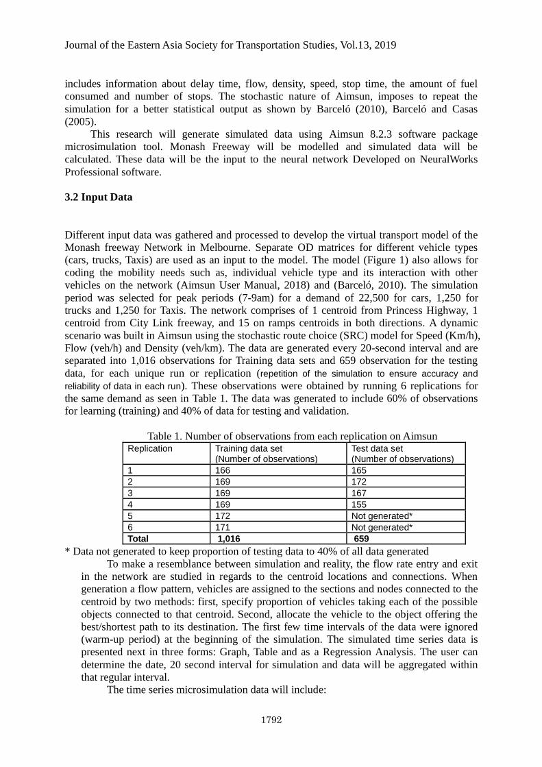
the same demand as seen in Table 1. The data was generated to include 60% of observations

for learning (training) and 40% of data for testing and validation.

Table 1. Number of observations from each replication on Aimsun Replication Training data set

(Number of observations) Test data set (Number of observations)

1 166 165 2 169 172 3 169 167 4 169 155

5 172 Not generated*

6 171 Not generated*

Total 1,016 659

* Data not generated to keep proportion of testing data to 40% of all data generated

To make a resemblance between simulation and reality, the flow rate entry and exit

in the network are studied in regards to the centroid locations and connections. When

generation a flow pattern, vehicles are assigned to the sections and nodes connected to the

centroid by two methods: first, specify proportion of vehicles taking each of the possible

objects connected to that centroid. Second, allocate the vehicle to the object offering the

best/shortest path to its destination. The first few time intervals of the data were ignored

(warm-up period) at the beginning of the simulation. The simulated time series data is

presented next in three forms: Graph, Table and as a Regression Analysis. The user can

determine the date, 20 second interval for simulation and data will be aggregated within

that regular interval.

The time series microsimulation data will include:


1793

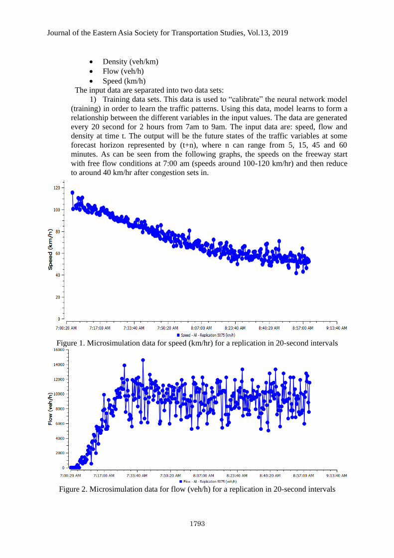
• Density (veh/km)

• Flow (veh/h)

• Speed (km/h)

The input data are separated into two data sets:

1) Training data sets. This data is used to “calibrate” the neural network model

(training) in order to learn the traffic patterns. Using this data, model learns to form a

relationship between the different variables in the input values. The data are generated

every 20 second for 2 hours from 7am to 9am. The input data are: speed, flow and

density at time t. The output will be the future states of the traffic variables at some

forecast horizon represented by (t+n), where n can range from 5, 15, 45 and 60

minutes. As can be seen from the following graphs, the speeds on the freeway start

with free flow conditions at 7:00 am (speeds around 100-120 km/hr) and then reduce

to around 40 km/hr after congestion sets in.

Figure 1. Microsimulation data for speed (km/hr) for a replication in 20-second intervals

Figure 2. Microsimulation data for flow (veh/h) for a replication in 20-second intervals


1794

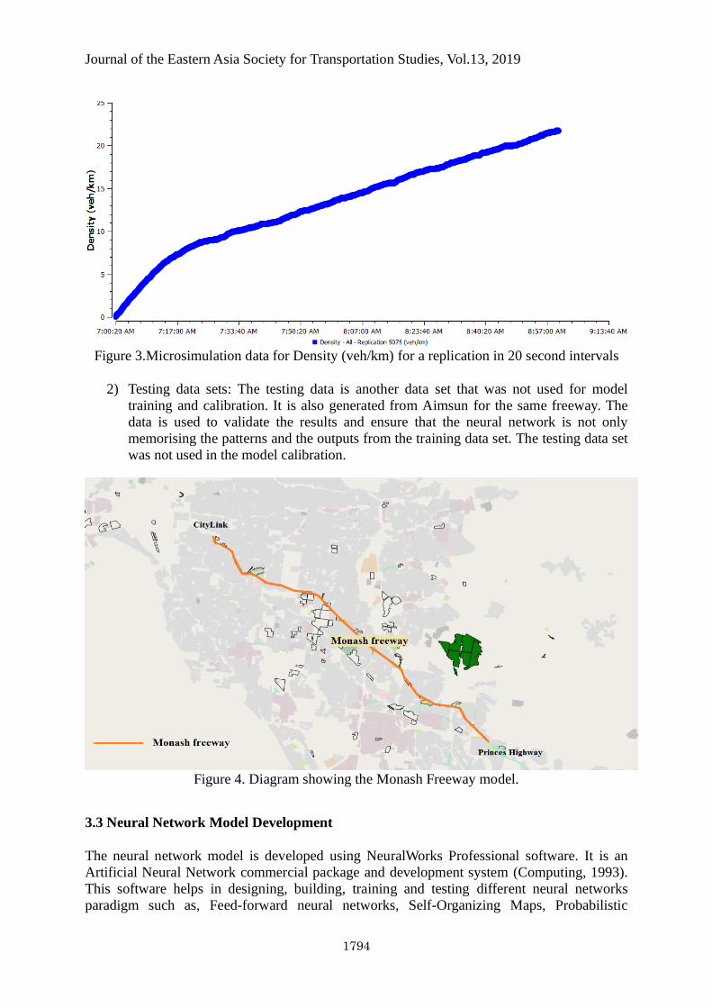
Figure 3.Microsimulation data for Density (veh/km) for a replication in 20 second intervals

2) Testing data sets: The testing data is another data set that was not used for model

training and calibration. It is also generated from Aimsun for the same freeway. The

data is used to validate the results and ensure that the neural network is not only

memorising the patterns and the outputs from the training data set. The testing data set

was not used in the model calibration.

Figure 4. Diagram showing the Monash Freeway model.

3.3 Neural Network Model Development

The neural network model is developed using NeuralWorks Professional software. It is an

Artificial Neural Network commercial package and development system (Computing, 1993).

This software helps in designing, building, training and testing different neural networks

paradigm such as, Feed-forward neural networks, Self-Organizing Maps, Probabilistic


1795

networks, etc. to solve complex, real-world problems. It has a very fine-grained control of the

parameters and architectures of each paradigm and contains extraordinary number of transfer

functions, learning rules, monitoring instrumentation, and other useful modelling tools. In this

Paper, the Backpropagation model is used to reduce predictive error. Backpropagation

algorithm Applies to model the deep neural networks. The term “backpropagation” referred to

when the error between the desired and the calculated output is reversed backwards to update

the weights. The procedure of training is as follows:

1) Perform forward propagation by calculating the output of the neural network.

2) Compute the error (cost function) between the targeted and the calculated output,

starting from the last layer back propagate to the first one.

3) Multiply the error from the third layer by the inputs in the second layer to calculate the

partial derivatives for this set of parameters.

4) send the error backwards to the previous hidden layer (L-1) and calculate the error

5) Calculate the partial deviation for this set of parameters.

6) Repeat 4-5 until reaching to the input layer.

7) Use the gradient descent to update the values of the weight.

8) Re-compute the forward propagation with the new weight following the steps from 1

to 7. The iteration cycle of the weights is called epoch. This process continue until an

optimal value is reached for the parameters.

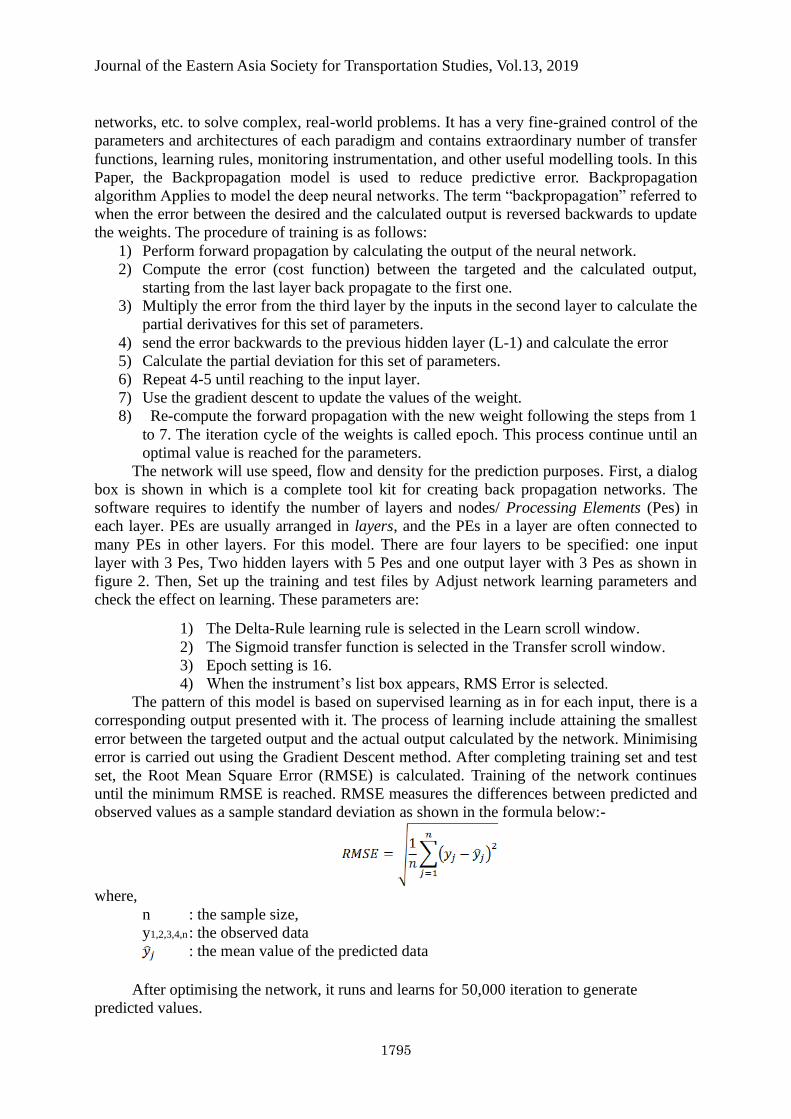
The network will use speed, flow and density for the prediction purposes. First, a dialog

box is shown in which is a complete tool kit for creating back propagation networks. The

software requires to identify the number of layers and nodes/ Processing Elements (Pes) in

each layer. PEs are usually arranged in layers, and the PEs in a layer are often connected to

many PEs in other layers. For this model. There are four layers to be specified: one input

layer with 3 Pes, Two hidden layers with 5 Pes and one output layer with 3 Pes as shown in

figure 2. Then, Set up the training and test files by Adjust network learning parameters and

check the effect on learning. These parameters are:

1) The Delta-Rule learning rule is selected in the Learn scroll window.

2) The Sigmoid transfer function is selected in the Transfer scroll window.

3) Epoch setting is 16.

4) When the instrument’s list box appears, RMS Error is selected.

The pattern of this model is based on supervised learning as in for each input, there is a

corresponding output presented with it. The process of learning include attaining the smallest

error between the targeted output and the actual output calculated by the network. Minimising

error is carried out using the Gradient Descent method. After completing training set and test

set, the Root Mean Square Error (RMSE) is calculated. Training of the network continues

until the minimum RMSE is reached. RMSE measures the differences between predicted and

observed values as a sample standard deviation as shown in the formula below:-

where,

n : the sample size,

y1,2,3,4,n : the observed data

: the mean value of the predicted data

After optimising the network, it runs and learns for 50,000 iteration to generate

predicted values.


1796

Figure 5. Predictive learning system representation.

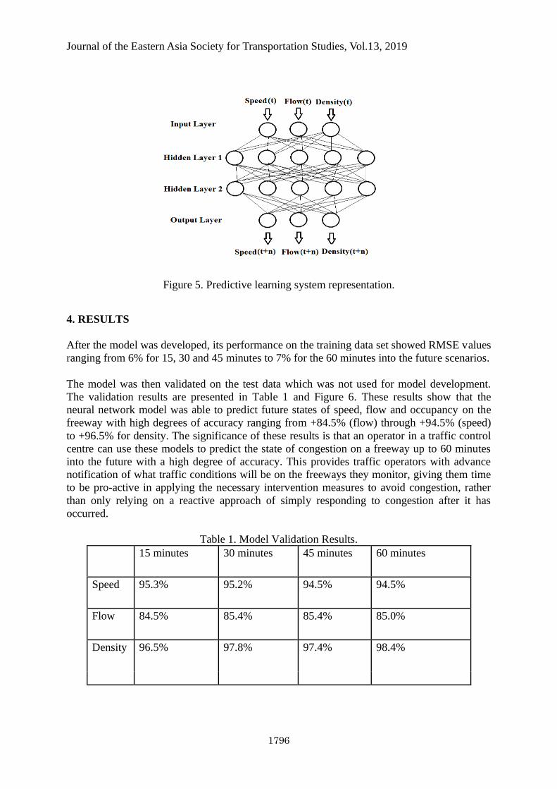
4. RESULTS

After the model was developed, its performance on the training data set showed RMSE values

ranging from 6% for 15, 30 and 45 minutes to 7% for the 60 minutes into the future scenarios.

The model was then validated on the test data which was not used for model development.

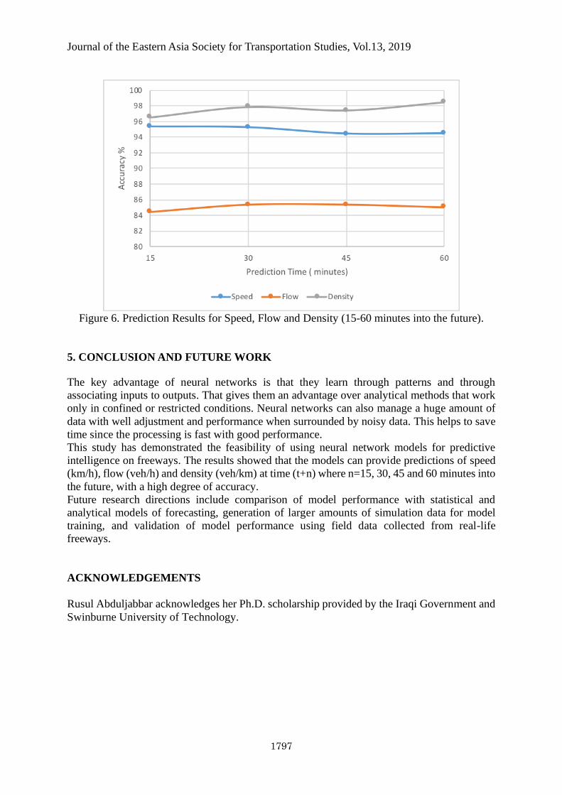
The validation results are presented in Table 1 and Figure 6. These results show that the

neural network model was able to predict future states of speed, flow and occupancy on the

freeway with high degrees of accuracy ranging from +84.5% (flow) through +94.5% (speed)

to +96.5% for density. The significance of these results is that an operator in a traffic control

centre can use these models to predict the state of congestion on a freeway up to 60 minutes

into the future with a high degree of accuracy. This provides traffic operators with advance

notification of what traffic conditions will be on the freeways they monitor, giving them time

to be pro-active in applying the necessary intervention measures to avoid congestion, rather

than only relying on a reactive approach of simply responding to congestion after it has

occurred.

Table 1. Model Validation Results. 15 minutes 30 minutes 45 minutes 60 minutes

Speed 95.3% 95.2% 94.5% 94.5%

Flow 84.5% 85.4% 85.4% 85.0%

Density 96.5% 97.8% 97.4% 98.4%


1797

Figure 6. Prediction Results for Speed, Flow and Density (15-60 minutes into the future).

5. CONCLUSION AND FUTURE WORK

The key advantage of neural networks is that they learn through patterns and through

associating inputs to outputs. That gives them an advantage over analytical methods that work

only in confined or restricted conditions. Neural networks can also manage a huge amount of

data with well adjustment and performance when surrounded by noisy data. This helps to save

time since the processing is fast with good performance.

This study has demonstrated the feasibility of using neural network models for predictive

intelligence on freeways. The results showed that the models can provide predictions of speed

(km/h), flow (veh/h) and density (veh/km) at time (t+n) where n=15, 30, 45 and 60 minutes into

the future, with a high degree of accuracy.

Future research directions include comparison of model performance with statistical and

analytical models of forecasting, generation of larger amounts of simulation data for model

training, and validation of model performance using field data collected from real-life

freeways.

ACKNOWLEDGEMENTS

Rusul Abduljabbar acknowledges her Ph.D. scholarship provided by the Iraqi Government and

Swinburne University of Technology.


1798

REFERENCES

1. Abdul jabbar, R., Dia, H., Liyanage, S. and Bagloee, S., 2019. Applications of

artificial intelligence in transport: An overview. Sustainability, 11(1), p.189.

2. AIMSUN 2018. Aimsun Version 8.3 User’s Manual, SYSTEMS, T. T. S. (ed.) 8.3 ed.

Barcelona, Spain.

3. AKGÜNGÖR, A. P. & DOĞAN, E. 2009. An artificial intelligent approach to traffic

accident estimation: model development and application. Transport, 24, 135-142.

4. ALETA, A. & MORENO, Y. 2018. Multilayer Networks in a Nutshell. arXiv preprint

arXiv:1804.03488.

5. ARETAKIS, N., ROUMELIOTIS, I., ALEXIOU, A., ROMESIS, C. &

MATHIOUDAKIS, K. 2015. Turbofan engine health assessment from flight data.

Journal of Engineering for Gas Turbines and Power, 137, 041203.

6. BARCELÓ, J. 2010. Fundamentals of traffic simulation, Springer.

7. BARCELÓ, J. & CASAS, J. 2005. Dynamic network simulation with AIMSUN.

Simulation approaches in transportation analysis. Springer.

8. BUDALAKOTI, S., SRIVASTAVA, A. N. & OTEY, M. E. 2009. Anomaly detection

and diagnosis algorithms for discrete symbol sequences with applications to airline

safety. IEEE TRANSACTIONS ON SYSTEMS, MAN, AND CYBERNETICS PART C,

APPLICATIons and reviews", 39, 101.

9. CHEN, Q., SONG, X., YAMADA, H. & SHIBASAKI, R. Learning Deep

Representation from Big and Heterogeneous Data for Traffic Accident Inference.

AAAI, 2016. 338-344.

10. COMPUTING, N. 1993. A Technology Handbook for Professional II/Plus and

NeuralWorks Explorer. Neural Ware, Pittsburgh, Pa.

11. DIA, H. 2001. An object-oriented neural network approach to short-term traffic

forecasting. European Journal of Operational Research, 131, 253-261.

12. DIA, H. & ROSE, G. 1997. Development and evaluation of neural network freeway

incident detection models using field data. Transportation Research Part C:

Emerging Technologies, 5, 313-331.

13. DOĞAN, E. & AKGÜNGÖR, A. P. 2013. Forecasting highway casualties under the

effect of railway development policy in Turkey using artificial neural networks.

Neural Computing and Applications, 22, 869-877.

14. HELD, M., KÜNG, L., ÇABUKOGLU, E., PARESCHI, G., GEORGES, G. &

BOULOUCHOS, K. Future mobility demand estimation based on sociodemographic

information: A data-driven approach using machine learning algorithms. 18th Swiss

Transport Research Conference (STRC 2018), 2018. STRC.

15. HUANG, W., SONG, G., HONG, H. & XIE, K. 2014. Deep architecture for traffic

flow prediction: deep belief networks with multitask learning. IEEE Transactions on

Intelligent Transportation Systems, 15, 2191-2201.

16. INFRASTRUCTURE AUSTRALIA, M. 2015. Australian infrastructure audit.

Australian Government Printing Service Canberra.

17. JIANG, H., ZOU, Y., ZHANG, S., TANG, J. & WANG, Y. 2016. Short-Term Speed

Prediction Using Remote Microwave Sensor Data: Machine Learning versus

Statistical Model. Mathematical Problems in Engineering, 2016, 1-13.

18. LEDOUX, C. 1997. An urban traffic flow model integrating neural networks.

Transportation Research Part C: Emerging Technologies, 5, 287-300.

19. LEVENE, J., LITMAN, S., SCHILLINGER, I. & TOOMEY, C. 2018. How advanced

analytics can benefit infrastructure capital planning [Online]. Mckinsey & Company


1799

(Capital Projects & Infrastructure). [Accessed March, 2018 2018].

20. LI, B., ZHANG, D., SUN, L., CHEN, C., LI, S., QI, G. & YANG, Q. Hunting or

waiting? Discovering passenger-finding strategies from a large-scale real-world taxi

dataset. Pervasive Computing and Communications Workshops (PERCOM

Workshops), 2011 IEEE International Conference on, 2011. IEEE, 63-68.

21. LIAO, S., ZHOU, L., DI, X., YUAN, B. & XIONG, J. Large-scale short-term urban

taxi demand forecasting using deep learning. Proceedings of the 23rd Asia and

South Pacific Design Automation Conference, 2018. IEEE Press, 428-433.

22. Liyanage, S., Dia, H., Abduljabbar, R. and Bagloee, S., 2019. Flexible Mobility

On-Demand: An Environmental Scan. Sustainability, 11 (5): 1262.

23. LINKINGMELBOURNE 2018. METROPOLITAN TRANSPORT PLAN.

Melbourne, Australia.

24. LV, Y., DUAN, Y., KANG, W., LI, Z. & WANG, F.-Y. 2014. Traffic Flow Prediction

With Big Data: A Deep Learning Approach. IEEE Transactions on Intelligent

Transportation Systems, 1-9.

25. MAHAMUNI, A. 2018. Internet of Things, machine learning, and artificial

intelligence in the modern supply chain and transportation. Defense Transportation

Journal.

26. MORE, R., MUGAL, A., RAJGURE, S., ADHAO, R. B. & PACHGHARE, V. K.

Road traffic prediction and congestion control using Artificial Neural Networks.

Computing, Analytics and Security Trends (CAST), International Conference on,

2016. IEEE, 52-57.

27. MUKAI, N. & YODEN, N. 2012. Taxi demand forecasting based on taxi probe data

by neural network. Intelligent Interactive Multimedia: Systems and Services.

Springer.

28. NUZZOLO, A. & COMI, A. 2016. Advanced public transport and intelligent

transport systems: new modelling challenges. Transportmetrica A: Transport Science,

12, 674-699.

29. REN, H., SONG, Y., WANG, J., HU, Y. & LEI, J. A Deep Learning Approach to the

Citywide Traffic Accident Risk Prediction. 2018 21st International Conference on

Intelligent Transportation Systems (ITSC), 2018. IEEE, 3346-3351.

30. SAHRAOUI, A.-E.-K. & JAYAKRISHNAN, R. 2005. Microscopic-macroscopic

models systems integration: A simulation case study for ATMIS. Simulation, 81,

353-363.

31. TAAMNEH, M., ALKHEDER, S. & TAAMNEH, S. 2017. Data-mining techniques

for traffic accident modeling and prediction in the United Arab Emirates. Journal of

Transportation Safety & Security, 9, 146-166.

32. THEOFILATOS, A., YANNIS, G., KOPELIAS, P. & PAPADIMITRIOU, F. 2016.

Predicting Road Accidents: A Rare-events Modeling Approach. Transportation

Research Procedia, 14, 3399-3405.

33. VASAVI, S. 2018. Extracting Hidden Patterns Within Road Accident Data Using

Machine Learning Techniques. Information and Communication Technology.

Springer.

34. WANG, R., FAN, S. & WORK, D. B. 2016. Efficient multiple model particle filtering

for joint traffic state estimation and incident detection. Transportation Research Part

C: Emerging Technologies, 71, 521-537.

35. WANG, R. & WORK, D. B. Interactive multiple model ensemble Kalman filter for

traffic estimation and incident detection. Intelligent Transportation Systems (ITSC),

2014 IEEE 17th International Conference on, 2014. IEEE, 804-809.


1800

36. WEI, W., JIA, X., LIU, Y. & YU, X. Travel Time Forecasting with Combination of

Spatial-Temporal and Time Shifting Correlation in CNN-LSTM Neural Network.

Asia-Pacific Web (APWeb) and Web-Age Information Management (WAIM) Joint

International Conference on Web and Big Data, 2018. Springer, 297-311.

37. WU, Y., TAN, H., QIN, L., RAN, B. & JIANG, Z. 2018. A hybrid deep learning

based traffic flow prediction method and its understanding. Transportation Research

Part C: Emerging Technologies, 90, 166-180.

38. WYSOCKI, A. & ŁAWRYŃCZUK, M. Jordan neural network for modelling and

predictive control of dynamic systems. Methods and Models in Automation and

Robotics (MMAR), 2015 20th International Conference on, 2015. IEEE, 145-150.

39. YAO, H., WU, F., KE, J., TANG, X., JIA, Y., LU, S., GONG, P., YE, J. & LI, Z. Deep

multi-view spatial-temporal network for taxi demand prediction. Thirty-Second

AAAI Conference on Artificial Intelligence, 2018.

Predictive Intelligence: A Neural Network Learning System ...

Documents

Transcript of Predictive Intelligence: A Neural Network Learning System ...