Prediction with Mixture Models - publishup.uni-potsdam.de · die Parameter des Modells nutzlic he...
58
Institut f¨ ur Informatik Professur Maschinelles Lernen Prediction with Mixture Models Kumulative Dissertation zur Erlangung des akademischen Grades “doctor rerum naturalium” (Dr. rer. nat.) in der Wissenschaftsdisziplin Informatik eingereicht an der Mathematisch-Naturwissenschaftlichen Fakult¨ at der Universit¨ at Potsdam von Dipl.-Inf. Peter Haider Potsdam, den 7. August 2013
Transcript of Prediction with Mixture Models - publishup.uni-potsdam.de · die Parameter des Modells nutzlic he...

Institut fur InformatikProfessur Maschinelles Lernen
Prediction with Mixture Models
Kumulative Dissertation
zur Erlangung des akademischen Grades“doctor rerum naturalium”
(Dr. rer. nat.)in der Wissenschaftsdisziplin Informatik
eingereicht an derMathematisch-Naturwissenschaftlichen Fakultat
der Universitat Potsdam
vonDipl.-Inf. Peter Haider
Potsdam, den 7. August 2013

Published online at the Institutional Repository of the University of Potsdam: URL http://opus.kobv.de/ubp/volltexte/2014/6961/ URN urn:nbn:de:kobv:517-opus-69617 http://nbn-resolving.de/urn:nbn:de:kobv:517-opus-69617

Abstract
Learning a model for the relationship between the attributes and the annotated labelsof data examples serves two purposes. Firstly, it enables the prediction of the label forexamples without annotation. Secondly, the parameters of the model can provide usefulinsights into the structure of the data. If the data has an inherent partitioned structure, itis natural to mirror this structure in the model. Such mixture models predict by combiningthe individual predictions generated by the mixture components which correspond to thepartitions in the data. Often the partitioned structure is latent, and has to be inferredwhen learning the mixture model. Directly evaluating the accuracy of the inferred partitionstructure is, in many cases, impossible because the ground truth cannot be obtained forcomparison. However it can be assessed indirectly by measuring the prediction accuracyof the mixture model that arises from it. This thesis addresses the interplay between theimprovement of predictive accuracy by uncovering latent cluster structure in data, andfurther addresses the validation of the estimated structure by measuring the accuracy ofthe resulting predictive model.
In the application of filtering unsolicited emails, the emails in the training set are latentlyclustered into advertisement campaigns. Uncovering this latent structure allows filtering offuture emails with very low false positive rates. In order to model the cluster structure, aBayesian clustering model for dependent binary features is developed in this thesis.
Knowing the clustering of emails into campaigns can also aid in uncovering which emailshave been sent on behalf of the same network of captured hosts, so-called botnets. Thisassociation of emails to networks is another layer of latent clustering. Uncovering this latentstructure allows service providers to further increase the accuracy of email filtering and toeffectively defend against distributed denial-of-service attacks. To this end, a discriminativeclustering model is derived in this thesis that is based on the graph of observed emails. Thepartitionings inferred using this model are evaluated through their capacity to predict thecampaigns of new emails.
Furthermore, when classifying the content of emails, statistical information about thesending server can be valuable. Learning a model that is able to make use of it requirestraining data that includes server statistics. In order to also use training data where theserver statistics are missing, a model that is a mixture over potentially all substitutionsthereof is developed.
Another application is to predict the navigation behavior of the users of a website. Here,there is no a priori partitioning of the users into clusters, but to understand different usagescenarios and design different layouts for them, imposing a partitioning is necessary. Thepresented approach simultaneously optimizes the discriminative as well as the predictivepower of the clusters.
Each model is evaluated on real-world data and compared to baseline methods. The
results show that explicitly modeling the assumptions about the latent cluster structure
leads to improved predictions compared to the baselines. It is beneficial to incorporate a
small number of hyperparameters that can be tuned to yield the best predictions in cases
where the prediction accuracy can not be optimized directly.
2

Zusammenfassung
Das Lernen eines Modells fur den Zusammenhang zwischen den Eingabeattributen undannotierten Zielattributen von Dateninstanzen dient zwei Zwecken. Einerseits ermoglichtes die Vorhersage des Zielattributs fur Instanzen ohne Annotation. Andererseits konnendie Parameter des Modells nutzliche Einsichten in die Struktur der Daten liefern. Wenndie Daten eine inharente Partitionsstruktur besitzen, ist es naturlich, diese Struktur imModell widerzuspiegeln. Solche Mischmodelle generieren Vorhersagen, indem sie die in-dividuellen Vorhersagen der Mischkomponenten, welche mit den Partitionen der Datenkorrespondieren, kombinieren. Oft ist die Partitionsstruktur latent und muss beim Lernendes Mischmodells mitinferiert werden. Eine direkte Evaluierung der Genauigkeit der in-ferierten Partitionsstruktur ist in vielen Fallen unmoglich, weil keine wahren Referenzdatenzum Vergleich herangezogen werden konnen. Jedoch kann man sie indirekt einschatzen,indem man die Vorhersagegenauigkeit des darauf basierenden Mischmodells misst. DieseArbeit beschaftigt sich mit dem Zusammenspiel zwischen der Verbesserung der Vorhersage-genauigkeit durch das Aufdecken latenter Partitionierungen in Daten, und der Bewertungder geschatzen Struktur durch das Messen der Genauigkeit des resultierenden Vorhersage-modells.
Bei der Anwendung des Filterns unerwunschter E-Mails sind die E-Mails in der Train-ingsmende latent in Werbekampagnen partitioniert. Das Aufdecken dieser latenten Struk-tur erlaubt das Filtern zukunftiger E-Mails mit sehr niedrigen Falsch-Positiv-Raten. Indieser Arbeit wird ein Bayes’sches Partitionierunsmodell entwickelt, um diese Partition-ierungsstruktur zu modellieren.
Das Wissen uber die Partitionierung von E-Mails in Kampagnen hilft auch dabei her-auszufinden, welche E-Mails auf Veranlassen des selben Netzes von infiltrierten Rechnern,sogenannten Botnetzen, verschickt wurden. Dies ist eine weitere Schicht latenter Parti-tionierung. Diese latente Struktur aufzudecken erlaubt es, die Genauigkeit von E-Mail-Filtern zu erhohen und sich effektiv gegen verteilte Denial-of-Service-Angriffe zu vertei-digen. Zu diesem Zweck wird in dieser Arbeit ein diskriminatives Partitionierungsmodellhergeleitet, welches auf dem Graphen der beobachteten E-Mails basiert. Die mit diesemModell inferierten Partitionierungen werden via ihrer Leistungsfahigkeit bei der Vorhersageder Kampagnen neuer E-Mails evaluiert.
Weiterhin kann bei der Klassifikation des Inhalts einer E-Mail statistische Informa-tion uber den sendenden Server wertvoll sein. Ein Modell zu lernen das diese Informatio-nen nutzen kann erfordert Trainingsdaten, die Serverstatistiken enthalten. Um zusatzlichTrainingsdaten benutzen zu konnen, bei denen die Serverstatistiken fehlen, wird ein Modellentwickelt, das eine Mischung uber potentiell alle Einsetzungen davon ist.
Eine weitere Anwendung ist die Vorhersage des Navigationsverhaltens von Benutzerneiner Webseite. Hier gibt es nicht a priori eine Partitionierung der Benutzer. Jedochist es notwendig, eine Partitionierung zu erzeugen, um verschiedene Nutzungsszenarien zuverstehen und verschiedene Layouts dafur zu entwerfen. Der vorgestellte Ansatz optimiertgleichzeitig die Fahigkeiten des Modells, sowohl die beste Partition zu bestimmen als auchmittels dieser Partition Vorhersagen uber das Verhalten zu generieren.
Jedes Modell wird auf realen Daten evaluiert und mit Referenzmethoden verglichen. Die
Ergebnisse zeigen, dass das explizite Modellieren der Annahmen uber die latente Partition-
ierungsstruktur zu verbesserten Vorhersagen fuhrt. In den Fallen bei denen die Vorhersage-
genauigkeit nicht direkt optimiert werden kann, erweist sich die Hinzunahme einer kleinen
Anzahl von ubergeordneten, direkt einstellbaren Parametern als nutzlich.
3

Contents
1 Introduction 61.1 Mixture Models . . . . . . . . . . . . . . . . . . . . . . . . . . . . . . 61.2 Classifying Emails with Mixtures of Campaigns . . . . . . . . . . . . 81.3 Predicting Email Campaigns Using a Botnet Model . . . . . . . . . . 91.4 Classifying Emails with Missing Values . . . . . . . . . . . . . . . . . 101.5 Predicting User Behavior in Different Market Segments . . . . . . . . 11
2 Bayesian Clustering for Email Campaign Detection 142.1 Introduction . . . . . . . . . . . . . . . . . . . . . . . . . . . . . . . . 142.2 Bayesian Clustering for Binary Features . . . . . . . . . . . . . . . . 152.3 Feature Transformation . . . . . . . . . . . . . . . . . . . . . . . . . . 162.4 Parameter Estimation . . . . . . . . . . . . . . . . . . . . . . . . . . 172.5 Sequential Bayesian Clustering . . . . . . . . . . . . . . . . . . . . . . 172.6 Email Campaign Detection . . . . . . . . . . . . . . . . . . . . . . . . 182.7 Related Work . . . . . . . . . . . . . . . . . . . . . . . . . . . . . . . 202.8 Conclusion . . . . . . . . . . . . . . . . . . . . . . . . . . . . . . . . . 21
3 Finding Botnets Using Minimal Graph Clusterings 223.1 Introduction . . . . . . . . . . . . . . . . . . . . . . . . . . . . . . . . 223.2 Problem Setting and Evaluation . . . . . . . . . . . . . . . . . . . . . 233.3 Minimal Graph Clustering . . . . . . . . . . . . . . . . . . . . . . . . 243.4 Case Study . . . . . . . . . . . . . . . . . . . . . . . . . . . . . . . . 273.5 Conclusion and Discussion . . . . . . . . . . . . . . . . . . . . . . . . 283.6 Acknowledgments . . . . . . . . . . . . . . . . . . . . . . . . . . . . . 29
4 Learning from Incomplete Data with Infinite Imputations 304.1 Introduction . . . . . . . . . . . . . . . . . . . . . . . . . . . . . . . . 304.2 Problem Setting . . . . . . . . . . . . . . . . . . . . . . . . . . . . . . 314.3 Learning from Incomplete Data in One Step . . . . . . . . . . . . . . 324.4 Solving the Optimization Problem . . . . . . . . . . . . . . . . . . . . 324.5 Example Learners . . . . . . . . . . . . . . . . . . . . . . . . . . . . . 344.6 Empirical Evaluation . . . . . . . . . . . . . . . . . . . . . . . . . . . 354.7 Conclusion . . . . . . . . . . . . . . . . . . . . . . . . . . . . . . . . . 37
5 Discriminative Clustering for Market Segmentation 385.1 Introduction . . . . . . . . . . . . . . . . . . . . . . . . . . . . . . . . 385.2 Related Work . . . . . . . . . . . . . . . . . . . . . . . . . . . . . . . 395.3 Discriminative Segmentation . . . . . . . . . . . . . . . . . . . . . . . 40
4

5.4 Empirical Evaluation . . . . . . . . . . . . . . . . . . . . . . . . . . . 435.5 Conclusion . . . . . . . . . . . . . . . . . . . . . . . . . . . . . . . . . 45
6 Discussion 476.1 Application-oriented Modelling . . . . . . . . . . . . . . . . . . . . . 496.2 Improvement of Predictive Power . . . . . . . . . . . . . . . . . . . . 496.3 Evaluability . . . . . . . . . . . . . . . . . . . . . . . . . . . . . . . . 50
5

Chapter 1
Introduction
In many applications, one wants to annotate instances of data with labels that in-dicate how to further process them. Examples include email messages, where theservice provider wants to know whether to move them to a special folder becausethey are unsolicited (spam), or transmit them normally. In cases where obtainingthe labels for all instances by other means is too costly or impractical, one can learna model for the relationship between the examples’ attributes and their labels. Forthat, the learner usually needs a much smaller set of examples where both the at-tributes and labels are known. In the following, let x denote the attributes of anexample, y a label, θ the parameters of a model, and c a cluster of instances. Ingeneral, the learner is given a training set X = (x1, y1), . . . , (xn, yn), where the xispecify the attributes of the i-th example, and the yi the respective labels. The goalis to infer a prediction model P (y|x; θ), parameterized by some set of parameters θ.The latter are usually optimized according to the accuracy of the prediction modelon the training data. After that, the model can be used to predict the labels y ofnew examples. Sometimes the predictions themselves are not relevant, but only themodel parameters that serve as a way to interprete or explain the training data. Buteven in these cases, the predictions on new data are useful because their accuracyprovides an indicator for the appropriateness of the model parameters.
1.1 Mixture Models
Mixture models are a class of prediction models that rely on an underlying partitionstructure in the relationship between attributes and label. They have an advantage ofexhibiting greater complexity than their underlying single-component models, whilein many cases, retaining their same efficient inference methods. For example, learninga linear classifier using a convex loss function can be done very efficiently, but thediscriminative power of linear models is too low in some applications. A commonapproach to increasing the discriminative power is to map the examples into a higher-dimensional feature space and learn a decision funtion in the feature space. If theobjective function is quadratically regularized, the solution can be expressed solelyin terms of inner products of examples in the feature space, and thus the mappingdoes not have to be done explicitly, but rather the inner product may be defineddirectly as a kernel function. The resulting decision function can then be non-linearin the input examples. However kernel methods are usually much slower than linearmethods, because evaluating the decision function requires iterating over potentially
6

all training examples. But there already exists a partitioning of the training set intocomponents, learning a linear classifier for each component is easy, and the resultingmixture model is then effectively non-linear. Especially if the data actually exhibitan albeit unknown cluster structure, taking this structure into account when learninga predictive model can be advantageous.
Examples of successful uses of mixture models include speech recognition [Povey 10],clustering of gene expression microarray data [McNicholas 10], modeling the returnsof financial assets [Geweke 11], and image segmentation [Zhang 11].
In general, the partitioning of the training set is not given, hence the task has twoparts. Firstly, the learner has to find a partioning C consisting of clusters c1, . . . , cm,such that
⋃ci = X and ∀i 6= j : ci ∩ cj = ∅. Secondly, for each cluster, one has
to estimate its predictive model parameters θ. They can be either estimated in amaximum-a-posteriori fashion,
θ∗ = arg maxθP (θ)P (y|x; θ),
P (y|x) = P (y|x; θ∗),
or they can be integrated out in order to perform full Bayesian inference:
P (y|x) =
∫P (θ)P (y|x; θ)dθ.
While the latter is more exact, the former is used in cases when full Bayesian inferenceis computationally intractable.
Within a component c, the mixture model defines a distribution P (y|x; c) be-cause each component is associated with a set of parameters θ. The component-wisedistributions can be combined by summing over the components, weighted by theirprobabilities given input x,
P (y|x) =∑
c
P (c|x)P (y|x; c). (1.1)
Assessing the predictive accuracy of the resulting distribution P (y|x) indirectlyallows one to evaluate the performance of the partitioning C. Although there is nodeterministic relationship between the two, in general a higher accuracy of P (y|x)requires a higher accuracy of C. Of course, in simple settings this relationship breaksdown; for example, if the output can be predicted from the input completely inde-pendent from the cluster structure. But we focus on applications where there is infact a latent cluster structure in the data, and where knowing to which cluster anexample belongs facilitates the prediction of its output.
This thesis is concerned with the interplay between two mutually dependent pro-cesses: the one hand the improvement of predictive accuracy by uncovering the latentmixture structure in the data, and the validation of the estimated mixture structureby measuring the accuracy of the resulting predictive model. It is not only of interestto evaluate a particular estimated clustering, but also to evaluate different methodsof estimating clusterings. In particular, several new methods for estimating mixturemodels from training data are presented. The aim of the methods is to forgo un-justified assumptions about the data and to enable direct optimization of predictiveaccuracy when possible. This results in a clear relationship between the resultingpredictive accuracy and the validity of the produced clusterings, setting the methodsapart from previously published clustering approaches where there is, in general, nopossibility to assess the partitionings inferred from real-world data.
7

1.2 Classifying Emails with Mixtures of Campaigns
In the application of spam filtering, the inputs x are the contents of emails andsometimes additional meta-data. The label that is to be predicted is binary, y ∈−1, 1, representing non-spam or spam. The most common way to represent thecontent of an email is to use a bag-of-words representation of the text and use abinary indicator vector that has a component for each word in the vocabulary. Thusthe vector x consists of ones that correspond to words that are included in the emailand zeroes elsewhere. Due to the high dimensionality of the input vectors and thelarge number of training examples, usually generalized linear models are used tomodel P (y|x). Let w be the vector of same dimensionality as x parameterizing thedistribution, and g an arbitrary link function such that g−1 : R→ [−1; 1]. Then thepredictive distribution is defined as
P (y|x;w) = g−1(w>x).
To guarantee very low false positive rates, an email provider wants to train a con-servative spam filter, which does not try to capture the essence of “spamness”, butinstead filters only emails that belong to a known spam campaign. This is not pos-sible using a single generalized linear model since those result in a planar decisionboundary, and thus all emails that lie between the known spam campaigns in inputspace are filtered as well. A remedy is to combine several linear classifiers, one foreach campaign of spam emails. Since the probability that a message is spam giventhat it belongs to a spam capaign is one, Equation 1.1 can be written as
P (y = 1|x) =
∑c∈C P (x|c)P (c)
P (x). (1.2)
The main challenge is to find a clustering C of a training set X into campaigns.We do this by constructing a Bayesian mixture model over emails in a transformedfeature space in which the dimensions are treated as independent:
P (X|C) =∏
c∈C
∫
θ
P (θ)∏
x∈c
P (φ(x)|θ)dθ. (1.3)
Here, θ is the parameter vector that governs the distribution over transformed fea-ture vectors within a cluster, and φ is the transformation mapping. It is an injectiveBoolean function, constructed with the goal to minimize the negative influence ofthe independence assumption for the transformed feature dimensions. Previous ap-proaches for modeling the generative process of text data fall into two categories. Thefirst category of approaches is to include an independence assumption in the inputspace which is clearly unjustified and harms performance. The second possibility isto use an n-gram model which inflates the dimensionality of the data and thereforesuffers from the problem that the overwhelming majority of n-grams have never beenseen before in the training set.
Using a multivariate Beta distribution for the prior P (θ) yields a closed-formsolution for the integral in Equation 1.3, and we can find a good approximative solu-tion to the clustering problem arg maxC P (X|C) efficiently using a greedy sequentialalgorithm.
8

It is problematic to estimate P (c) in Equation 1.2 from training data, because theactivities of spam campaigns can change rapidly within short timeframes. Thus weassume a uniform distribution over campaigns. This could lead to the overestimationof P (y = 1|x) for messages from campaigns that are split over multiple clustersby the clustering process. To correct for this, we replace the sum over campaignsby the maximum over campaigns. Finally, the constant 1/|C| from the uniformdistribution over clusters can be omitted, since we are only concerned with the relativeprobabilities of messages being spam compared to each other. This leads us to thefinal classification score as
score(x) =maxc∈C P (x|c)
P (x).
In this application, not only the predictions of the final model are of interest, butalso the clustering itself has intrinsic value. It provides insight into the behavior ofspammers: it can tell us about how often the campaign templates change, how manydifferent campaigns are active at any given time, and about the employed strategiesfor dissemination.
This approach is detailed and evaluated by Haider and Scheffer [Haider 09]. Thepaper makes three major contributions. The most import contribution is the gen-erative model for a clustering of binary feature vectors, based on a transformationof the inputs into a space in which an independence assumption induces minimumapproximation error. Furthermore, the paper presents an optimization problem forlearning the transformation together with an appropriate algorithm. And finally itdetails a case study on real-world data that evaluates the clustering solution on emailcampaign detection.
For the paper I, derived the generative model and the feature transformation,proved the theorem, developed and implemented the algorithms and conducted theexperiments.
1.3 Predicting Email Campaigns Using a Botnet
Model
In this application, the prediction of email campaigns is mainly a method to evaluatethe accuracy of the clustering. We are given a set of emails, consisting of their sender’sIP address x and their spam campaign y. The goal is to find a clustering C of the pairs(x, y), such that the clusters correspond to the botnets on whose behalf the emailswere sent. Knowing which IP address belongs to which botnet at any time facilitiatesthe defense against distributed denial-of-service (DDOS) attacks. However, thereis no ground truth available with which to assess an inferred clustering. But byevaluating the prediction of campaigns given IP addresses and a current clustering,we can indirectly compare different methods of clustering emails into botnets. Themore accurate the clustering C, the more accurate the predictive distribution that isbased on the clustering tends to be:
P (y|x;C) =∑
c∈C
P (y|x; c)P (c|x).
9

We make the assumption that the campaign of an email is conditionally independentof its IP address given its cluster; i.e., P (y|x; c) = P (y|c). Both the distributionover campaigns within a botnet P (y|c) and the distribution over botnets given anIP address can be straightforwardly estimated using a maximum-likelihood approach.The main challenge is again to find the clustering C of a given set of training pairs. Weconstruct a discriminative model P (C|(x1, y1), . . . , (xn, yn)) that represents its inputas a graph of emails, where there is an edge between two emails if and only if they arefrom the same campaign or IP address. The crucial observation is that edges presentin the graph provide weak evidence for two emails belonging to the same botnet,whereas the absence of an edge only provides very weak evidence against it. Ourmodel thus is defined purely in terms of the cliques of the graph. Within each clique,we define the posterior distribution of the partitioning of the emails of the cliqueto follow the Chinese Restarant Process (CRP). The individual clique distributionsare then multiplied and normalized. Since there is no closed-form solution for thefull Bayesian approach of averaging over all clusterings for predicting campaigns, wedevise a blockwise Gibbs sampling scheme that, in the limit of an infinite numberof iterations, generates samples C1, . . . , CT from the true posterior. Predictions arethen averaged over the generated samples, such that the final predictive distributionis
P (y|x;C1, . . . , CT ) =∑
t
∑
c∈Ct
P (c|x,Ct)P (y|c).
This approach is detailed and evaluated by Haider and Scheffer [Haider 12b]. Thepaper contributes a discriminative model for clustering in a graph without makingdistributional assumptions about the generative process of the observables. Addi-tionally, it presents a Gibbs sampling algorithm with which to efficiently traverse thestate graph to generate unbiased samples from the posterior in the limit. Finally, itreports on a case study with data from an email service provider.
For the paper, I formulated the problem setting, derived the probabilistic model,proved the theorems, developed and implemented the algorithm, and conducted theexperiments.
1.4 Classifying Emails with Missing Values
In spam filtering, one can use additional meta-information z about an email in addi-tion to its content x, such as statistics about the sending server. Yet because we wantto utilize training data from external sources that do not include these statistics, weare faced with the problem of learning a classifier from examples with missing values.At test time, the server statistics are always available.
The way to do this without introducing simplifications is to find a set of imputa-tions1 Ω = ω1, . . . , ωD for the missing values. Each ωd is a complete instantiationof the meta-information of all examples, and restricted to z in places where the truemeta-information is known. We prove that using at most n different sets of impu-tations, where n is the size of the training set, is equivalent to using a mixture of
1In the area of learning from data with missing values, the assumed values are usually calledimputations.
10

infinitely many imputation sets. We assume a known prior distribution P (ω) over im-putations. It can, for example, represent the belief that imputed values are normallydistributed about the mean of the actual values of other examples in the same featuredimension. Unlinke previous work, our approach finds a complete distribution overall possible imputations, instead of finding only a single imputation for each example.
The ωd correspond to the components of a mixture model. Their respective pre-dictive distributions P (y|x, z;ω) can be modeled and learned as a conventional binaryclassification problem. We choose a decision function kernelized with a Mercer kernelk,
f(x, z) =∑
i
αiyik(x, z, xi, ω),
where all mixture components share the same dual multipliers αi.Thus the task is to simultaneously estimate the multipliers αi and the weights
β1, . . . , βD of the individual mixture components. The most concise way to do thisis to construct a joint optimization problem, where both are free parameters andthe objective function is defined in terms of the classification error on the trainingexamples, the prior knowledge P (ω) about the imputations, and a regularizer on thenorm of the weight vector in feature space. This amounts to optimizing
arg minα,β,ω
∑
i
lh(yi,∑
j
αjyj∑
d
βdk(xi, ωd,i, xj, ωd,j)
+ λ∑
i,j,d
αiαjβdk(xi, ωd,i, xj, ωd,j)
+ λ′∑
d
βd logP (ωd),
where lh(y, f) = max(1−yf, 0) is the hinge loss, under the constraints that ∀d : βd ≥ 0and
∑d βd = 1. It can be solved in its dual form using a min-max-procedure that
iteratively selects the next best set of imputations ωd and its weight βd and thenre-adjusts the multipliers αi.
This approach is detailed and evaluated by Dick et al. [Dick 08]. The novelcontributions of this paper are as follows. Firstly, it presents an optimization problemfor learning a predictor from incomplete data that makes only minimal assumptionsabout the distribution of the missing attribute values, and allows potentially infintelymany imputations. Secondly, it contains a proof that the optimal solution can beexpressed in terms of a finite number of imputations. On multiple datasets it showsthat the presented method consistently outperforms single imputations.
For this paper I developed the theoretical framework and the optimization prob-lems, and proved the theorem. Uwe Dick implemented the algorithm and conductedthe experiments.
1.5 Predicting User Behavior in Different Market
Segments
In the final application, the predictions of the learned mixture model are only ofsecondary importance to the prediction model itself. Training examples consist of
11

attributes x and behavior y. The goal is to simultaneously find a set of k marketsegments with associated parameters θ1, . . . , θk, and a classifier h : X → 1, . . . , k.The classifier sorts each example into one of the segments, given its attributes. Thesegment parameters are supposed to predict the behavior of the examples in thesegment, and thus serve as a description of the segment. For example, in the domainof user behavior on a website, each example corresponds to one browsing session.Its attributes are the timestamp, the referrer domain, and the category of the firstpageview. Its behavior is represented by the categories of the subsequent pageviewsand the layout elements in which the clicked links reside. Given a set of segments ofthe training examples, one can craft specific website layouts for each segment, whichcater best to the included browsing sessions’ preferences. New sessions can then beclassified using h into one of the segments and presented with the correspondinglayout.
The operator of the website wants the classifier to accurately discriminate exam-ples given only their attributes, and also wants the segment parameters to predictthe behavior of all examples that are classified into it with high accuracy. Therefore,first finding a clustering in the space of attributes and then selecting parameters foreach cluster is not advisable because it can result in poor prediction of the behavior.Analogously, first computing a clustering in the space of behaviors leads to good pre-dictions of the behavior within each cluster, but can gravely harm the capability ofany classifier to separate examples into the respective clusters where their behavioris best predicted. The appropriate optimization problem is thus
arg maxh,θ
∑
i
logP (yi|θh(xi)). (1.4)
The premise here is that the predictive distribution family P (y|θ) is chosen so that theparameters θ can be interpreted in a meaningful way to guide the design of segmentedmarketing strategies. Additionally, estimating the parameters within a segment cgiven the contained examples with indices i ∈ c has to be efficient. For example,if the behavior is an exchangeable sequence of mutually independent multinomialvariables the optimization problem
arg maxθ
∑
i∈c
logP (yi|θ)
has a closed-form solution, and the parameters θ of the segment can be interpreted asthe preferences of the members of the segment. Our approach stands in contrast topreviously published market segmentation methods. Instead of defining a priori cri-teria for clustering the examples, we simultaneously optimize the clustering accordingto the goals of separability and homogeneity.
Solving the optimization problem of Equation 1.4 in the straightforward mannerof alternating between optimizing h and θ does not work in practice because it getsstuck in poor local optima where, in most cases, the majority of segments are empty.As a remedy, we develop an algorithm that relies on the expression of the parametersof h as a function of the parameters θ. The resulting objective function can bemaximized approximately using a variant of the EM-algorithm.
This approach is detailed and evaluated by Haider et al. [Haider 12a]. Thepaper presents the first concise optimization problem for market segmentation, which
12

consists of learning a classifier and component-wise predictors. An algorithm forapproximately solving the problem is detailed, and evaluated on a large-scale datasetof user navigation behavior of a news website.
For the paper I formulated the problem setting and the optimization problem,derived the approximate solution, developed and implemented the algorithms, andconducted the main experiments. Luca Chiarandini preprocessed the data and im-plemented and conducted the baseline experiments.
13

Bayesian Clustering for Email Campaign Detection
Peter Haider [email protected] Scheffer [email protected]
University of Potsdam, Department of Computer Science, August-Bebel-Strasse 89, 14482 Potsdam, Germany
Abstract
We discuss the problem of clustering elementsaccording to the sources that have generatedthem. For elements that are characterizedby independent binary attributes, a closed-form Bayesian solution exists. We derive asolution for the case of dependent attributesthat is based on a transformation of the in-stances into a space of independent featurefunctions. We derive an optimization prob-lem that produces a mapping into a spaceof independent binary feature vectors; thefeatures can reflect arbitrary dependencies inthe input space. This problem setting is mo-tivated by the application of spam filteringfor email service providers. Spam traps de-liver a real-time stream of messages known tobe spam. If elements of the same campaigncan be recognized reliably, entire spam andphishing campaigns can be contained. Wepresent a case study that evaluates Bayesianclustering for this application.
1. Introduction
In model-based clustering, elements X =x(1), . . . ,x(n) have been created by an unknownnumber of sources; each of them creates elementsaccording to its specific distribution. We studythe problem of finding the most likely clustering ofelements according to their source
C∗ = argmaxC
P (X|C), (1)
where C consistently partitions the elements of X intoclusters C = c1, . . . , cm that are mutually exclusiveand cover each element.
Appearing in Proceedings of the 26 th International Confer-ence on Machine Learning, Montreal, Canada, 2009. Copy-right 2009 by the author(s)/owner(s).
Computing the likelihood of a set X under a cluster-ing hypothesis C requires the computation of the jointlikelihood of mutually dependent elements Xc withina partition c. This is usually done by assuming latentmixture parameters θ that generate the elements ofeach cluster and imposing a prior over the mixture pa-rameters. The joint likelihood is then an integral overthe parameter space, where individual likelihoods areindependent given the parameters:
P (Xc) =
∫ ∏
x∈Xc
P (x|θ)P (θ)dθ. (2)
For suitable choices of P (x|θ) and P (θ), this integralhas an analytic solution. In many cases, however,the space X of elements is very high-dimensional, andthe choice of likelihood and prior involves a trade-offbetween expressiveness of the generative model andtractability regarding the number of parameters. If theelements are binary vectors, X = 0, 1D, one extremewould be to model P (x|θ) as a full multinomial distri-bution over X , involving 2D parameters. The otherextreme is to make an independence assumption onthe dimensions of X , reducing the model parametersto a vector of D Bernoulli probabilities. No remedy forthis dichotomy is known that preserves the existenceof an analytic solution to the integral in Equation 2.
Our problem setting is motivated by the applicationof clustering messages according to campaigns; thiswill remain our application focus throughout the pa-per. Filtering spam and phishing messages reliablyremains a hard problem. Email service providers op-erate Mail Transfer Agents which observe a stream ofincoming messages, most of which have been createdin bulk by a generator. A generator can be an appli-cation that dispatches legitimate, possibly customizednewsletters, or a script that creates spam or phishingmessages and disseminates them from the nodes of abotnet. Mail Transfer Agents typically blacklist knownspam and phishing messages. Messages known to bespam can be collected by tapping into botnets, andby harvesting emails in spam traps. Spam traps areemail addresses published invisibly on the web that
14

Bayesian Clustering for Email Campaign Detection
have no legitimate owner and can therefore not re-ceive legitimate mail. In order to avoid blacklisting,spam dissemination tools produce emails according toprobabilistic templates. This motivates our problemsetting: If all elements that are generated in a jointcampaign can be identified reliably, then all instancesof that campaign can be blacklisted as soon as oneelement reaches a spam trap, or is delivered from aknown node of a botnet. Likewise, all instances of anewsletter can be whitelisted as soon as one instanceis confirmed to be legitimate.
While text classification methods are frequently re-ported to achieve extremely high accuracy for spamfiltering under laboratory conditions, their practicalcontribution to the infrastructure of email services issmaller: they are often applied to decide whether ac-cepted emails are to be delivered to the inbox or thespam folder. The vast majority of all spam delivery at-tempts, however, is turned down by the provider basedon known message and IP blacklists. Text classifiersare challenged with continuously shifting distributionsof spam and legitimate messages; their risk of falsepositives does not approach zero sufficiently closely toconstitute a satisfactory solution to the spam problem.
This paper makes three major contributions. Firstly,we develop a generative model for a clustering of bi-nary feature vectors, based on a transformation of theinput vectors into a space in which an independenceassumption incurs minimal approximation error. Thetransformations can capture arbitrary dependenciesin the input space while the number of parametersstays reasonable and full Bayesian inference remainstractable. Secondly, we derive the optimization prob-lem and algorithm that generates the feature transfor-mation. Finally, we present a large-scale case studythat explores properties of the Bayesian clustering so-lution for email campaign detection.
The paper is structured as follows. We present theBayesian clustering model in Section 2, and an opti-mization problem and algorithm for transforming de-pendent features into independent features in Section3. Section 4 discusses the estimation of prior param-eters, Section 5 develops a sequential clustering algo-rithm based on Bayesian decisions. Section 6 reportson empirical results in our motivating application. Wereview related work in Section 7. Section 8 concludes.
2. Bayesian Clustering for BinaryFeatures
In general, a clustering hypothesis C entails that thelikelihood of the dataset factorizes into the likelihoods
of the subsets Xc of elements in the clusters c ∈ C.Elements within a cluster are dependent, so the like-lihood of each element depends on the preceding ele-ments in its cluster, as in Equation 3.
P (X|C) =∏
c∈CP (Xc)
=∏
c∈C
∏
i:x(i)∈cP (x(i)|x(j) ∈ c : j < i) (3)
The crucial part is modeling the probability P (x|X ′)of a binary feature vector x given a set of elements X ′.A natural way is to introduce latent model parametersθ and integrate over them as in Equation 4.
P (x|X ′) =∫
θ
P (x|θ)P (θ|X ′)dθ (4)
Modeling θ as a full joint distribution over all 2D pos-sible feature vectors, with D being the dimensionalityof the input space X , is intractable.Let φe be independent binary features and let vectorφ(x) be a representation of x in the space of inde-pendent features φ. In order to streamline the pre-sentation of the clustering model, we postpone the ra-tionale and construction of the feature transformationto Section 3. Under the assumption that attributesin the space φ are independent, the model parame-ters can be represented as a vector of Bernoulli proba-bilities, θ ∈ (0, 1)E , and we can compute P (x|θ) as∏Ee=1 P (φe(x)|θe). Furthermore, we impose a Beta
prior on every component θe with parameters αe andβe. Since the Beta distribution is conjugate to theBernoulli distribution, we can now compute the poste-rior over the model parameters analytically as in Equa-tion 5, where #e = |x′ ∈ X ′ : φe(x′) = 1|.
P (θ|X ′) = P (X ′|θ) P (θ)P (X ′)
=
∏Ee=1
∏x∈X′ P (φe(x)|θe)PBeta(θe|αe, βe)∫
P (X ′|θ′)P (θ′)dθ′
=
E∏
e=1
PBeta(θe|αe +#e, βe + |X| −#e) (5)
The integral in Equation 4 then has the analytic solu-tion of Equation 6:
P (x|X ′) =∏
e:φe(x)=1
αe +#e
αe + βe + |X ′| (6)
∏
e:φe(x)=0
βe + |X ′| −#e
αe + βe + |X ′| .
15

Bayesian Clustering for Email Campaign Detection
For a single element, independent of all others, theprobability term simplifies to
P (x) =∏
e:φe(x)=1
αeαe + βe
∏
e:φe(x)=0
βeαe + βe
. (7)
Furthermore, the joint probability of an interdepen-dent set X ′ in one cluster can be computed as
P (X ′) =∏
i:x(i)∈X′
P (x(i)|x(j) ∈ X ′ : j < i)
=E∏
e=1
∏#e
k=1(αe + k − 1)∏|X′|−#e
k=1 (βe + k − 1)∏|X′|k=1(αe + βe − 1)
=E∏
e=1
B(αe +#e, βe + |X ′| −#e)
B(αe, βe),
where B denotes the Beta function.
3. Feature Transformation
In this section we will present a method of approx-imating a distribution over high-dimensional binaryvectors that allows analytical integration over the in-duced model parameters. The idea is to find a map-ping into another space of binary vectors where the di-mensions are treated independently of each other, suchthat the divergence between the original distributionand the approximate distribution defined in terms ofthe mapped vectors is minimal.
A straightforward approach would be to employ amodel that captures dependencies between small setsof attributes only and assumes independence other-wise. Instead of working with independence assump-tions, we construct a search space of transformations.This space is complete in the sense that any possi-ble interaction of attributes can be reflected in thenewly constructed attributes. These attributes areconstructed such that their product approximates thetrue distribution as closely as possible.
The Bayesian clustering model introduced in Section 2requires us to infer the probability of a feature vectorx given a set of feature vectors X ′ it depends on. Wetherefore want to approximate P (x|X ′) by a quantityQφ(x|X ′), where φ is a mapping from the original vec-tor space X = 0, 1D to the image space Z = 0, 1E .We define Qφ as a product over independent probabil-ities for each output dimension, as in Equation 8.
Qφ(x|X ′) =E∏
e=1
P (φe(x)|φe(X ′)) (8)
By its definition as a product over probabilities, quan-tity Qφ(x|X) is always non-negative; however, it does
not necessarily sum to one over the event space ofpossible inputs x. Since Qφ serves as an approxi-mation of a probability in the Bayesian inference, itis desirable that
∑xQφ(x|X) ≤ 1 for all X. More-
over, the natural measure of approximation quality –the Kullback-Leibler divergence – is only motivatedfor measures that add up to at most one and maybe maximized by trivial solutions otherwise. Notethat the sum does not have to be exactly 1, sincean extra element x with P (x) = 0 can be addedto X that absorbs the remaining probability mass,
Qφ(x|X ′)def= 1−∑
x∈X Qφ(x|X ′).
Normalization ofQφ(x|X) is intractable, since it wouldrequire explicit summation of Equation 8 over all 2D
possible input elements. We therefore have to definethe space of possible transformations such that afterany transformationQφ is guaranteed to sum to at mostone. By Theorem 1 (see Appendix), this holds for allinjective transformations.
Every mapping from X = 0, 1D to the Z = 0, 1Ecan be represented as a set of E Boolean functions,and every Boolean function can be constructed as acombination of elementary operations. Therefore wecan define the search space as the set of all concate-nations of elementary Boolean transformations ψ thatpreserve injectiveness. The choice of which elementarytransformations to use is driven by the practical goalthat φ also preserves sparseness. The following twoelementary transformations are injective, sufficient togenerate any Boolean function, and preserve sparsity:
ψxij((. . . , xi, . . . , xj , . . . )>)=(. . . , xi, . . . , xi 6= xj , . . . )
>
ψaij((. . . , xi, . . . , xj , . . . )>)
=(. . . , xi∧xj , . . . , xi∧¬xj ,¬xi∧xj , . . . )>.
Every ψ replaces two features by Boolean combina-tions thereof, leaving every other feature untouched.
For any set of elements X, the quantity Qφ(x|X)should minimize the Kullback-Leibler divergence fromthe true distribution P (x|X). Hence, the optimizationcriterion (Equation 9) is the expected KL divergencebetween Qφ(x|X) and P (x|X) over all X.
φ∗ =argminφ
EX∼P(x)
[KL(P (·|X)||Qφ(·|X))] (9)
= argminφ
EX∼P(x)
[∑
x∈XP (x|X) log
P (x|X)
Qφ(x|X)
](10)
= argmaxφ
EX∼P(x)
[∑
x∈XP (x|X) logQφ(x|X)
](11)
= argmaxφ
EX∼P(x),x∼P(x|X)
[logQφ(x|X)] . (12)
16

Bayesian Clustering for Email Campaign Detection
Equation 10 expands the definition of the KL diver-gence; Equation 11 replaces minimization by maxi-mization and drops the term P (x|X) logP (x|X) whichis constant in φ. We approximate the expectation inEquation 12 by the sum over an empirical sample S,and obtain
Optimization Problem 1. Over the set of con-catenations of elementary transformations, φ ∈ψxij , ψaij∗, maximize
∑
x∈SlogQφ(x|S \ x).
The sum of log-probabilities can be calculated as
∑
x∈SlogQφ(x|S \ x)
=
E∑
e=1
#Se log(α0 +#S
e −1)− |S| log(α0 +β0 + |S| −1)
+ (|S| −#Se ) log(β0 + |S| −#S
e − 1),
where #Se = |x′ ∈ S : φe(x
′) = 1|, and α0, β0 arethe parameters of the Beta prior.
Optimization Problem 1 is non-convex, so we apply agreedy procedure that iteratively adds the next-besttransformation starting with the identity transforma-tion, as detailed in Algorithm 1.
Algorithm 1 Greedy Transformation Composition
φ0 ← idfor t = 1 . . . doψ ← argmaxψ
∑x∈S Qφt−1ψ(x|S \ x)
if∑x∈S
Qφt−1ψ(x|S \ x) <∑x∈S
Qφt−1(x|S \ x)thenreturn φt−1
elseφt ← φt−1 ψ
end ifend for
4. Parameter Estimation
In the following section, we will derive a closed-formestimator for parts of the parameters of the prior P (θ).The decisions whether to merge an element x with aset X ′ depend strongly on the prior parameters viaP (x) in Equation 7 and P (x|X ′) in Equation 6.
Heller and Ghahramani (2005) derive an EM-like algo-rithm that maximizes the data likelihood by iteratively
finding the best clustering and then performing gradi-ent descent on the prior parameters. This approachis computationally very expensive, since the likelihoodfunction is not convex and the entire dataset needs tobe re-clustered in each iteration.
We overcome these problems by using an alternativeparametrization of the Beta distribution. This allowsus to estimate half of the parameters from an unclus-tered set of training examples S; the other half of theparameters is pooled into a single value and adjustedby a grid search on tuning data.
We re-parametrize the Beta priors as αe = µeσ andβe = (1−µe)σ, where the µe are the prior means and σis the common precision1 parameter. The probabilityof an element not given any other elements of the samecluster does not depend on the prior precisions, only onthe means. Hence, the means have a stronger impacton the resulting partitioning.
Imposing a Beta-distributed hyperprior on µe with pa-rameters α0 > 1 and β0 > 1 we can compute theMaximum-A-Posteriori estimate of the means as
µe = argmaxµ
P (µ|S) = argmaxµ
∏
x∈SP (φe(x)|µ)P (µ)
= argmaxµ
PBeta (µ|α0 + |x ∈ S : φe(x) = 1|,
β0 + |x ∈ S : φe(x) = 0|)
=α0 + |x ∈ S : φe(x) = 1| − 1
α0 + β0 + |S| − 2.
5. Sequential Bayesian Clustering
In this section we discuss the task of inferring the mostlikely partitioning of a set of emails and present ourmodel-based sequential clustering algorithm.
Brute-force search over the entire space of possi-ble partitionings in Equation 1 requires the evalua-tion of exponentially many clusterings and is there-fore intractable for reasonable numbers of emails.A more efficient approach would be to performMarkov chain Monte Carlo sampling methods like in(Williams, 2000), which yields not only the Maximum-A-Posteriori partitioning, but samples from the poste-rior distribution.
Approximate agglomerative clustering algorithms(Heller & Ghahramani, 2005) are more efficient. Sincein practice emails have to be processed sequentially,and decisions whether an email belongs to a spam cam-paign cannot be revised after delivering it, we adoptthe sequential clustering algorithm of Haider et al.
1The precision parameter of a Beta distribution is in-versely related to its variance.
17

Bayesian Clustering for Email Campaign Detection
Algorithm 2 Model-based Sequential Clustering
C ← for t = 1 . . . n docj ← argmaxc∈C P (x(t)|Xc)if P (x(t)|Xc) < P (x(t)) thenC ← C ∪ x(t)
elseC ← C \ cj ∪ cj ∪ x(t)
end ifend forreturn C
(2007). This greedy incremental algorithm has theadvantage of approximately finding the best campaignassociation of a new email in O(n), where n is thenumber of previously seen emails, instead of takingO(n3) operations for performing a full agglomerativere-clustering.
Instead of a weighted similarity measure as in (Haideret al., 2007), our clustering model is based on a genera-tive model. We replace the weighted sum over pairwisefeatures by an integral over the model parameters ofa cluster. This gives us the model-based sequentialclustering in Algorithm 2.
In every step, the algorithm compares the hypothe-ses that the new element belongs to one of the exist-ing clusters with the hypothesis that it forms its owncluster. The likelihoods of these hypotheses are cal-culated according to Equations 6 and 7. This greedyalgorithm can be straightforwardly extended to usinga non-uniform prior over clustering hypotheses, by re-placing P (x) with P (x)P (C∪x(t)) and P (x(t)|Xc)with P (x(t)|Xc)P (C \ cj ∪ cj ∪ x(t)).
6. Email Campaign Detection
In this section, we explore the behavior of the featuretransformation procedure, and conduct a case studyof the Bayesian clustering method for spam filtering.
In unsupervised clustering, there is no ground truthavailable that the output of the clustering algorithmcan be compared with. Fortunately, our motivatingapplication scenario – email spam containment – hasa natural evaluation criterion: the contribution of theproduced partitionings to accurate filtering.
We design an experimental setting that evaluates theBayesian clustering solution and the feature transfor-mation technique for the problem of detecting spamcampaigns at an email service provider. Benchmarkdata sets such as the SpamTREC corpus are not suit-able for our evaluation. A fair evaluation relies on a
stream that contains realistic proportions of messagesof mailing campaigns, in the correct chronological or-der. Benchmark corpora contain messages that havebeen received by users, and have therefore passed un-known filtering rules employed by the receiving server.Furthermore, benchmark data sets do not contain re-liable time stamps whereas the actual chronologicalorder is crucial.
Our experimental setting relies on a stream of spammessages received by the mail transfer agent of anemail service provider. Between July and November2008, we recorded a small fraction of spam messages,a total of 139,250 spam messages in correct chronologi-cal order. The messages have been tagged as spam be-cause the delivering agent was listed on the SpamhausIP block list which is maintained manually. We sim-ulate the practical setting where one has a stream ofverified spams, and one stream of unknown emails, bytaking every other email from the set as training exam-ple. The rest is split into test examples (90%) and tun-ing examples. In order to maintain the users’ privacy,we blend the stream of spam messages with an addi-tional stream of 41,016 non-spam messages from pub-lic sources. The non-spam portion contains newslet-ters and mailing lists in correct chronological order aswell as Enron emails and personal mails from publiccorpora which are not necessarily in chronological or-der. Every email is represented by a binary vector of1,911,517 attributes that indicate the presence or ab-sence of a word. The feature transformation techniqueintroduces an additional 101,147 attributes.
6.1. Feature Transformation
In order to assess the capability of our feature trans-formation technique for approximating a high dimen-sional probability distribution, we train the transfor-mation on an additional set S1 of 10,000 older emailsincluding spam and ham (i.e., non-spam) messages inequal parts, and test on another set S2 of emails ofthe same size. Since we cannot measure the Kullback-Leibler divergence from the true distribution directly,we measure the quantity −1
|Si|∑
x∈SilogQφ(x|Si\x),
which is the average entropy of an email, given all otheremails of the set. We compare the entropies on thetraining and test sets for the transformation found bythe Greedy Transformation Composition algorithm tothe entropy of the identity transformation. The iden-tity transformation corresponds to an assumption ofindependent attributes in the input space.
In addition to the overall optimal transformation, wecompute the optimal transformations φa and φx com-posed of only elementary transformations of the forms
18

Bayesian Clustering for Email Campaign Detection
ψaij or ψxij , respectively. Preliminary experimentsshowed that the choice of prior parameters α0 and β0has negligible influence within reasonable ranges, sowe report the results for α0 = 1.1 and β0 = 100 inTable 1. We can see that including elementary trans-
Table 1. Comparison of training and test entropies usingdifferent feature transformations.Transformation id φ∗ φa φx
Training entropy 1013.7 574.1 585.3 632.4Test entropy 1007.1 687.5 672.0 720.2
formations of the form ψxij decreases training entropy,but increases test entropy. The best transformationreduces test entropy compared to the identity trans-formation by about 33%. This shows that factorizingthe probability over the dimensions in the image spaceyields a much better approximation than factorizingover the dimensions in the original feature space.
6.2. Bayesian Clustering for Spam Filtering
Our evaluation protocol is as follows. We use a train-ing window of 5,000 known spam messages, corre-sponding to a history of approximately 11 days. Thetraining messages are partitioned using Algorithm 2.In each step, the clustering algorithm adds the chrono-logically next 100 known spam emails to the partition-ing and removes the 100 oldest. We then classify the100 next test messages. We use the odds ratio
maxXspamP (x|Xspam)
P (x)
as classification score, the maximum is over all spamclusters in the training window. Test messages are notadded to the window of partitioned training messages.
A main difficulty in spam filtering is that ham emailscan be very diverse, and it is unrealistic that one hastraining examples available from every region of thetrue distribution. We conduct experiments in twodifferent settings that assess performance when hamemails from the test distribution are available and theperformance without access to ham emails, respec-tively. In setting A, we train the feature transforma-tion and parameters µe with 10,000 ham emails fromthe test distribution, and in setting B, we train on10,000 spam messages instead.
As baseline for setting A, we use a Support VectorMachine that is trained in every step on the history ofthe last 5,000 spam and on the same 10,000 ham emailsas the clustering method. Hence, the SVM baselinereceives the same training data. In setting B, we use
a one-class SVM, trained on the history of 5,000 spammessages. Additionally, we evaluate the benefit of thefeature transformation by comparing with a clusteringalgorithm that uses the identity transformation.
An EM clustering procedure that uses a point esti-mates for the model parameters serves as an additionalreference. We use a MAP estimate based on the samemodel prior used for the Bayesian model. EM requiresthe number of clusters to be known. We use the num-ber of clusters that the Bayesian model identifies asinput to the EM clustering.
We use two evaluation measures. Firstly, we measurethe area under the ROC curve (AUC). Secondly, weuse an evaluation measure that reflects the character-istics of the application more closely. An MTA has tobe extremely confident when deciding to refuse a mes-sage for delivery from a contacting agent. We there-fore measure the rate of true positives (spam messagesidentified as such) at a false positive rate of zero. Weadjust the hyperparameters σ for the clustering modeland C or ν for the standard SVM and one-class SVM,respectively, on the tuning set. We tune the parame-ters separately for optimal AUC, and for an optimalrate of true positives at a false positive rate of zero.Figure 1 shows ROC curves.
We can see that in the setting with ham emails avail-able for training, the SVM outperforms the clustering-based filter in terms of AUC. In terms of the true pos-itive rate at a false positive rate of zero, the clusteringmethod outperforms the SVM classifier, by achievinga true positive rate of 0.945± 9.1× 10⁻⁴ compared to0.938±9.6×10⁻⁴ of the SVM. The cluster-based filtershows its full strength in setting B, in the absence ofnon-spam training messages from the test distribution.Here, it achieves an AUC value of 0.992 ± 2.6 × 10⁻⁴
and a true positive rate of 0.749± 1.7× 10⁻³, whereasthe one-class SVM attains an AUC of 0.770±1.4×10⁻³
and a true positive rate of 0.102 ± 1.2 × 10⁻³. Thatis, the Bayesian clustering method increases the truepositive rate at zero false positives almost sevenfold,in the setting where no training emails from the distri-bution of the test hams are available. Clustering withthe identity transformation as well as clustering withthe EM algorithm performs worse in all settings thanBayesian clustering with the feature transformation.In setting A (ham messages from the test distributionavailable) with the parameters tuned for a high truepositive rate at a false positive rate of zero, the EMalgorithm achieves a true positive rate of only 0.04.
19

Bayesian Clustering for Email Campaign Detection
0.75
0.8
0.85
0.9
0.95
1
0 0.05 0.1 0.15 0.2
Tru
e po
sitiv
e ra
te
False positive rate
With training hams, tuned for AUC
SVMClustering with φ=φa
Clustering with φ=idEM clustering 0.86
0.88
0.9
0.92
0.94
0.96
0.98
1
0x100 2x10⁻⁵ 4x10⁻⁵ 6x10⁻⁵ 8x10⁻⁵ 1x10⁻⁴
Tru
e po
sitiv
e ra
te
False positive rate
With training hams, tuned for TP at FP=0
Clustering with φ=φa
Clustering with φ=idSVM
0
0.2
0.4
0.6
0.8
1
0 0.02 0.04 0.06 0.08 0.1
Tru
e po
sitiv
e ra
te
False positive rate
No training hams, tuned for AUC
Clustering with φ=φa
Clustering with φ=idOne-class SVM
EM clustering 0
0.2
0.4
0.6
0.8
1
0x100 1x10⁻⁴ 2x10⁻⁴ 3x10⁻⁴
Tru
e po
sitiv
e ra
te
False positive rate
No training hams, tuned for TP at FP=0
Clustering with φ=φa
Clustering with φ=idOne-class SVM
EM clustering
Figure 1. Evaluation of spam filtering performance.
7. Related Work
Previous work on Bayesian clustering explored in greatdetail the use of hierarchical priors for the clusterstructure and algorithms for inference under such pri-ors, for example (Williams, 2000), (Heller & Ghahra-mani, 2005), and (Lau & Green, 2007). These ap-proaches focus on modeling hierarchical dependenciesbetween elements, while modeling only low-level de-pendencies between the attributes within elements,such as Gaussian covariances. By contrast, we assumea uniform prior over the cluster structure, and insteadfocus on modeling arbitrary dependencies between bi-nary attributes. We find that a non-uniform prior overpartitionings is in fact not necessary, because properlytaking the prior over mixture parameters P (θ) intoaccount also prevents the trivial solution of assigningevery element to its own cluster from being optimal.
Haider et al. (2007) devise a technique for mailingcampaign detection that relies on training data thatare manually clustered by campaigns. We find thatthe effort of manually partitioning training data into
clusters is prohibitive in practice. Note that the effortof partitioning data is much higher than the effort oflabeling data for classification because pairs of exam-ples have to be considered.
Multi-way dependencies between attributes have beenconsidered for instance by Zheng and Webb (2000) andWebb et al. (2005). They model the probability of anattribute vector as a product of conditional probabil-ities, such that each attribute can depend on multi-ple other attributes. If these approaches were to beused for Bayesian clustering, the number of mixtureparameters would grow exponentially in the degree ofdependencies. For our application, the high number ofattributes renders these approaches infeasible.
Remedies for the problem of constantly changing dis-tributions in the Spam filtering domain have been pro-posed in the area of adverserial learning. Teo et al.(2008) developed a formulation that allows to modeltest emails as modified versions of the training emailsand optimize the classifier against the worst-case sce-nario of modifications. This approach leads to classi-
20

Bayesian Clustering for Email Campaign Detection
fiers that are more robust against changes of the distri-bution of spam emails, but still require the availabilityof recent spam and ham training data.
8. Conclusion
We devised a model for Bayesian clustering of binaryfeature vectors. The model is based on a closed-form Bayesian solution of the data likelihood in whichthe model parameters are integrated out. It allowsfor arbitrary dependencies between the input features,by transforming them into a space in which treatingthem as independent incurs minimal approximation er-ror. We derived an optimization problem for learningsuch a transformation as a concatenation of elemen-tary Boolean operations. In order to estimate the pa-rameters of the prior from unlabeled data, we rewritethe parameters of the beta distribution in terms ofmean values and a common variance. The mean val-ues can be inferred in closed form from unlabeled dataefficiently, the common variance constitutes a param-eter that is adjusted on tuning data. We adapted asequential clustering algorithm to use it with Bayesianclustering decisions. In a case study, we observed thatthe Bayesian clustering solution achieves higher truepositive rates at a false positive rate of zero than anSVM. The benefit of the clustering solution is particu-larly visible when no non-spam training messages fromthe test distribution are available.
Acknowledgments
We gratefully acknowledge support from STRATORechenzentrum AG.
References
Haider, P., Brefeld, U., & Scheffer, T. (2007). Su-pervised Clustering of Streaming Data for EmailBatch Detection. Proceedings of the 24th Interna-tional Conference on Machine Learning (pp. 345–352).
Heller, K. A., & Ghahramani, Z. (2005). Bayesianhierarchical clustering. Proceedings of the 22nd In-ternational Conference on Machine Learning (pp.297–304).
Lau, J., & Green, P. (2007). Bayesian Model-BasedClustering Procedures. Journal of Computationaland Graphical Statistics, 16, 526–558.
Teo, C., Globerson, A., Roweis, S., & Smola, A.(2008). Convex Learning with Invariances. Ad-vances in Neural Information Processing Systems,20, 1489–1496.
Webb, G., Boughton, J., & Wang, Z. (2005). Not SoNaive Bayes: Aggregating One-Dependence Estima-tors. Machine Learning, 58, 5–24.
Williams, C. (2000). A MCMC approach to hierarchi-cal mixture modelling. Advances in Neural Infor-mation Processing Systems, 12, 680–686.
Zheng, Z., & Webb, G. (2000). Lazy Learning ofBayesian Rules. Machine Learning, 41, 53–84.
Appendix
Theorem 1. Let the implicit model parameter θe ofthe distribution P (ze) be Beta-distributed with param-eters αe and βe for each e ∈ 1, . . . , E. Then thequantity Qφ(x|X ′) as defined in Equation 8 sums toat most 1 for all X ′ iff φ is injective.
Proof. First we show indirectly that from ∀X ′ :∑z∈Z |x : φ(x) = z|∏E
e=1 P (ze|φe(X ′)) ≤ 1 fol-lows ∀z : |x : φ(x) = z| ≤ 1. Assume thatthere exists a z∗ ∈ Z with |x : φ(x) = z∗| ≥2. Then choose an x∗ with φ(x∗) = z∗. With-out loss of generality, let ∀e : z∗e = 1. Then setn = maxe
(E√0.5(αe + βe)− αe
)/(1− E√0.5
)+ 1 and
X∗ = x∗, . . . ,x∗ with |X∗| = n. It follows that
E∏
e=1
P (z∗e |φe(X∗)) =E∏
e=1
∫P (z∗e |θe)P (θe|φe(X∗))dθ
=
E∏
e=1
αe + n
αe + βe + n>
E∏
e=1
E√0.5 = 0.5,
and thus∑
z∈Z|x : φ(x) = z|
E∏
e=1
P (ze|φe(X∗))
≥|x : φ(x) = z∗|E∏
e=1
P (z∗e |φe(X∗)) > 1.
The opposite direction follows from the fact that ∀X ′ :∑z∈Z
∏Ee=1 P (ze|φe(X ′)) ≤ 1, because P (ze|φe(X ′))
is not an approximation, but a true Bayesian proba-bility. Now we have
∀X ′ :∑
x∈XQφ(x|X ′) ≤ 1
⇔∀X ′ :∑
x∈X
E∏
e=1
P (φe(x)|φe(X ′)) ≤ 1
⇔∀X ′ :∑
z∈Z|x : φ(x) = z|
E∏
e=1
P (ze|φe(X ′)) ≤ 1
⇔∀z : |x : φ(x) = z| ≤ 1⇔ φ is injective.
21

Finding Botnets Using Minimal Graph Clusterings
Peter Haider [email protected] Scheffer [email protected]
University of Potsdam, Department of Computer Science, August-Bebel-Str. 89, 14482 Potsdam, Germany
Abstract
We study the problem of identifying botnetsand the IP addresses which they comprise,based on the observation of a fraction of theglobal email spam traffic. Observed mail-ing campaigns constitute evidence for jointbotnet membership, they are represented bycliques in the graph of all messages. No evi-dence against an association of nodes is everavailable. We reduce the problem of identify-ing botnets to a problem of finding a minimalclustering of the graph of messages. We di-rectly model the distribution of clusteringsgiven the input graph; this avoids potentialerrors caused by distributional assumptionsof a generative model. We report on a casestudy in which we evaluate the model by itsability to predict the spam campaign that agiven IP address is going to participate in.
1. Introduction
We address the problem of identifying botnets that arecapable of exploiting the internet in a coordinated, dis-tributed, and harmful manner. Botnets consist of com-puters that have been infected with a software viruswhich allows them to be controlled remotely by a bot-net operator. Botnets are used primarily to dissemi-nate email spam, to stage distributed denial-of-service(DDoS) attacks, and to harvest personal informationfrom the users of infected computers (Stern, 2008).
Providers of computing, storage, and communicationservices on the internet, law enforcement and prose-cution are interested in identifying and tracking thesethreats. An accurate model of the set of IP addressesover which each existing botnet extends would make itpossible to protect services against distributed denial-
Appearing in Proceedings of the 29 th International Confer-ence on Machine Learning, Edinburgh, Scotland, UK, 2012.Copyright 2012 by the author(s)/owner(s).
of-service attacks by selectively denying service re-quests from the nodes of the offending botnet.
Evaluating botnet models is difficult, because theground truth about the sets of IP addresses that con-stitute each botnet at any given time is entirely un-available (Dittrich & Dietrich, 2008). Many studies onbotnet identification conclude with an enumeration ofthe conjectured number and size of botnets (Zhuanget al., 2008). Reliable estimates of the current sizeof one particular botnet require an in-depth analysisof the communication protocol used by the network.For instance, the size of the Storm botnet has beenassessed by issuing commands that require all activenodes to respond (Holz et al., 2008). However, oncethe communication protocol of a botnet is understood,the botnet is usually taken down by law enforcement,and one is again ignorant of the remaining botnets.
We develop an evaluation protocol that is guided bythe basic scientific principle that a model has to beable to predict future observable events. We focus onemail spam campaigns which can easily be observed bymonitoring the stream of messages that reach an emailservice provider. Our evaluation metric quantifies themodel’s ability to predict which email spam campaigna given IP address is going to participate in.
Previous studies have employed clustering heuristicsto aggregate IP addresses that participated in jointcampaigns into conjectured botnets (Xie et al., 2008;Zhuang et al., 2008). Because an IP address can be apart of multiple botnets during an observation inter-val, this approach is intrinsicaly inaccurate. The prob-lem is furthermore complicated as it is possible that abotnet processes multiple campaigns simultaneously,and multiple botnets may be employed for large cam-paigns. We possess very little background knowledgeabout whether multiple networks, each of which hasbeen observed to act in a coordinated way, really formone bigger, joint network. Also, distributional assump-tions about the generation of the observable events arevery hard to motivate. We address this lack of priorknowledge by directly modeling the conditional distri-
22

Finding Botnets Using Minimal Graph Clusterings
bution of clusterings given the observable data, andby searching for minimal clusterings that refrain frommerging networks as long as empirical evidence doesnot render joint membership in a botnet likely.
Other studies have leveraged different types of datain order to identify botnets. For example Mori et al.(2010); DiBenedetto et al. (2010) record and clusterfingerprints of the spam-sending hosts’ TCP behavior,exploiting that most bot types use their own protocolstacks with unique characteristics. Yu et al. (2010)identify bot-generated search traffic from query andclick logs of a search engine by detecting shifts inthe query and click distributions compared to a back-ground model. Another angle to detect bots is to mon-itor traffic from a set of potentially infected hosts andfind clusters in their outgoing and incoming packets(Gu et al., 2008; John et al., 2009); for example, DNSrequests of bots used to connect to control servers(Choi et al., 2009) or IRC channel activity (Goebel& Holz, 2007). The major difference here is that ac-cess to all the traffic of the hosts is required, and thusthese methods only work for finding infected hosts ina network under one’s control.
The rest of this paper is organized as follows. In Sec-tion 2, we discuss our approach to evaluating botnetmodels by predicting participation in spamming cam-paigns. In Section 3, we establish the problem of min-imal graph clustering, devise a probabilistic model ofthe conditional distribution of clusterings given theinput graph, and derive a Gibbs sampler. Section 4presents a case study that we carried out with an emailservice provider. Section 5 concludes.
2. Problem Setting and Evaluation
The ground truth about the sets of IP addresses thatconstitute each botnet is unavailable. Instead, we fo-cus on the botnet model’s ability to predict observableevents. We consider email spam campaigns which areone of the main activities that botnets are designedfor, and which we can easily observe by monitoring thestream of emails that reach an email service provider.Most spam emails are based on a campaign templatewhich is instantiated at random by the nodes of a bot-net. Clustering tools can identify sets of messages thatare based on the same campaign template with a lowrate of errors (Haider & Scheffer, 2009). A single cam-paign can be disseminated from the nodes of a singlebotnet, but it is also possible that a botnet processesmultiple campaigns simultaneously, and multiple bot-nets may be employed for large campaigns.
We formalize this setting as follows. Over a fixed pe-
riod of time, n messages are observed. An adjacencymatrix X of the graph of messages reflects evidencethat pairs of messages originate from the same bot-net. An edge between nodes i and j—represented byan entry of Xij = 1—is present if messages i and jhave been sent from the same IP address within thefixed time slice, or if a campaign detection tool hasassigned the messages to the same campaign cluster.Both types of evidence are uncertain, because IP ad-dresses may have been reassigned within the time sliceand the campaign detection tool may incur errors. Theabsence of an edge is only very weak and unreliable ev-idence against joint botnet membership, because thechance of not observing a link between nodes that arereally part of the same botnet is strongly dependenton the observation process.
The main part of this paper will address the problem ofinferring a reflexive, symmetric edge selector matrix Yin which entries of Yij = 1 indicate that the messagesrepresented by nodes i and j originate from the samebotnet. The transitive closure Y + of matrix Y definesa clustering CY of the nodes. The clustering placeseach set of nodes that are connected to one another bythe transitive closure Y + in one cluster; the clusteringis the union of clusters:
CY =⋃n
i=1j : Y +
ij = +1. (1)
Because Y + is reflexive, symmetric and transitive,it partitions all nodes into disjoint clusters; that is,c∩ c′ = ∅ for all c, c′ ∈ CY , and
⋃c∈CY
c = 1, . . . , n.An unknown process generates future messages whichare characterized by two observable and one latentvariable. Let the multinomial random variables s indi-cate the campaign cluster of a newly received message,a indicate the IP address, and let latent variable c indi-cate the originating cluster, associated with a botnet.We quantify the ability of a model CY to predict theobservable variable s of a message given a in terms ofthe likelihood
P (s|a,CY ) =∑
cP (s|c, CY )P (c|a,CY ). (2)
Equation 2 assumes that the distribution over cam-paigns is conditionally independent of the IP addressgiven the botnet; that is, botnet membership alonedetermines the distribution over campaigns.
Multinomial distribution P (s|c, CY ) quantifies thelikelihood of campaign s within the botnet c. It canbe estimated easily on training data because model CYfixes the botnet membership of each message. Multi-nomial distribution P (c|a,CY ) quantifies the probabil-ity that IP address a is part of botnet c given model
23

Finding Botnets Using Minimal Graph Clusterings
CY . Model CY assigns each node—that is, message—to a botnet. However, an address can be observedmultiple times within the fixed time slice, and the bot-net membership can change withing the time interval.Hence, a multinomial distribution P (c|a,CY ) has tobe estimated for each address a on the training data,based on the model CY . Note that at application time,P (c|a,CY ) and hence the right hand side of Equation2 can only be determined for addresses a that occur inthe training data on which CY has been inferred.
3. Minimal Graph Clustering
Let X be the adjacency matrix of the input graph withn nodes. Entries of Xij = 1 indicate an edge betweennodes i and j which constitutes uncertain evidence forjoint membership of these nodes in a botnet. The in-put matrix is assumed to be reflexive (Xii = 1 forall i), and symmetric (Xij = Xji).
The outcome of the clustering process is represented bya reflexive, symmetric edge selector matrix Y in whichentries of Yij = 1 indicate that nodes i and j are as-signed to the same cluster, which indicates that themessages originate from the same botnet. The tran-sitive closure Y + of matrix Y defines a clustering CYof the nodes according to Equation 1. Intuitively, theinput matrix X can be thought of as data, whereasoutput matrix Y should be thought of as the modelthat encodes a clustering of the nodes. A trivial base-line would be to use X itself as edge selector matrixY . In our application, this would typically lead to allmessages being grouped in one single cluster.
No prior knowledge is available on associations be-tween botnets in the absence of empirical evidence.If the adjacency matrix X does not contain evidencethat links nodes i and j, there is no justification forgrouping them into the same cluster. This is reflectedin the concept of a minimal edge selector matrix.
Definition 1. A selector matrix Y and, equivalently,the corresponding graph clustering CY , is minimalwith respect to adjacency matrix X if it satisfies
Y = Y + X, (3)
where (Y + X)ij = Y +ij Xij is the Hadamard product
that gives the intersection of the edges of Y + and X.
Intuitively, for every pair of nodes that are connectedby the adjacency matrix, selector matrix Y decideswhether they are assigned into the same cluster. Nodesthat are not connected by the adjacency matrix Xmust not be linked by Y , but can still end up in thesame cluster if they are connected by the transitive
closure Y +. Equation 3 also ensures that the transi-tive closure Y + does not differ from Y for any pair ofnodes i, j that are connected by the adjacency matrix.This enforces that no two different minimal selectormatrices have the same transitive closures and there-fore induce identical clusterings, which would inflatethe search space.
3.1. Probabilistic Model
This section derives a probabilistic model for the min-imal graph clustering problem. Its most salient prop-erty is that it is not based on a generative model ofthe graph, but instead directly models the conditionalprobability of the clustering given the adjacency ma-trix X. This circumnavigates systematic errors causedby inaccurate distributional assumptions for the gen-eration of the adjacency matrix X.
We define the posterior distribution over all reflexiveand symmetric matrices Y that are minimal with re-spect to X.
Definition 2. Let X ∈ 0, 1n×n be a reflexive andsymmetric adjacency matrix. Then, YX ⊆ 0, 1n×nis the set of matrices that are reflexive, symmetric, andminimal with respect to X.
In our application, each node is an element of at mosttwo cliques because each message is connected to allother messages that have been sent from the same IPaddress, and to all other messages that match the samecampaign template. If a template or an address hasbeen observed only once, either of these cliques mayresolve to just the node itself. Let QX denote theset of cliques in X, and let CqY be the projection ofclustering CY to the elements of q ∈ QX . Withineach clique q ∈ QX , any clustering CqY is minimalwith respect to X because Xij = 1 for all i, j ∈ q,and therefore any reflexive, symmetric, and transitiveclustering of q is possible. We model the probabilitydistribution over clusterings of each clique q ∈ QX as aChinese Restaurant process (Pitman & Picard, 2006)with concentration parameter αq > 0:
P (CqY |αq, nq) = α|Cq
Y |q
Γ(αq)
Γ(αq + nq)
∏
c∈CqY
Γ(|c|). (4)
Equation 5 now defines the distribution over all par-tition matrices Y ∈ YX as a product over all cliquesin QX , where the clique specific concentration param-eters are collected into α = αq : q ∈ QX.
P (CY |X,α) ∝ ∏q∈QX
P (CqY |αq, nq) if Y ∈ YX0 otherwise
(5)
24

Finding Botnets Using Minimal Graph Clusterings
Equation 5 can be seen in analogy to the factoriza-tion of the posterior over cliques in conditional ran-dom fields. However, because the minimality propertyhas non-local effects on the possible values that edgescan assume, this factorization is not equivalent to theassumption of the Markov property on which the fac-torization theorem for random fields is based (Ham-mersley & Clifford, 1971).
Normalization of Equation 5 is computationally in-tractable because it requires the enumeration of theelements of YX . However, the Gibbs sampler that wewill derive in the following only has to normalize overall values of the random variables that are reassignedin each step of the sampling process.
3.2. Inference
Computing the posterior distribution P (CY |X,α) isa generalization of the inference problem for conven-tional Chinese Restaurant process models. When allentries of X are one, the graph has only one clique andthe special case of a Chinese Restaurant process is ob-tained. In this case, depending on the concentrationparameter, the outcome may be one single cluster ofall nodes. Maximization of the posterior as well as fullBayesian inference are intractable even for this specialcase because of the non-convexity of the posterior andthe exponential number of possible clusterings. Hence,in this section we describe a Gibbs sampler that gen-erates unbiased samples from the posterior.
Algorithm 1 Assignment space YYi for Gibbs sampler
Input: Current partitioning matrix Y1: let q1, . . . , qk be the cliques with element i2: let Yi = ∅3: for all combinations c1 ∈ Cq1Y ∪ i, . . . ,ck ∈ CqkY ∪ i do
4: let Y ′−i = Y−i5: let Y ′il = Y ′li = 1 if and only if l ∈ cj for any j6: if (Y ′−i)
+ = Y ′−i then7: add Y ′ to YYi8: else9: discard Y ′
10: end if11: end forReturn: YYi , all reflexive, symmetric, minimal parti-
tioning matrices derived from Y by reassigning Yi.
Gibbs samplers divide the set of random variables intosmaller subsets and iteratively draw new values for onesubset given the values of the remaining variables. Forthe observations to form an unbiased sample, the ran-dom variables have to be partitioned such that the
sequence of assignments formes an ergodic Markovchain; that is, each state has to be reachable from eachother state. In our case, perhaps the most obvious-seeming approach would be to factor the posterior overindividual edges. However, since many matrices Y vi-olate the minimality condition, the chain of alterationsof single matrix entries would not in general be ergodic.
Therefore, we devise a sampling algorithm that jointlysamples the i-th row and column (the i-th row andcolumn are identical because Y is symmetric). Let Y ′irefer to the i-th row and column of the new matrixY ′, and let Y ′−i = Y−i refer to the remaining matrixentries, such that Y ′ = Y ′i ∪ Y ′−i. Equation 6 expandsthe definition of the conditional probability; Equation7 factorizes over the cliques, according to Equation 5.Equation 8 omits all terms that are constant in Y ′i :the denominator, and all cliques in which node i doesnot occur. Normalization of the right hand side ofEquation 8 is now over all values for Y ′i that render Y ′
reflexive, symmetric, and minimal with respect to X.
P (Y ′i |Y−i, X,α) =P (Y ′i , Y
′−i|X,α)
P (Y−i|X,α)(6)
∝∏q∈QX
P (CqY ′ |αq, nq)P (Y−i|X,α)
(7)
∝∏
q∈QX :i∈qP (CqY ′ |αq, nq) (8)
The main computational challenge here is to determinethe set YYi of reflexive, symmetric, minimal matricesthat can be derived from Y by changing row and col-umn i. Since Equation 8 has to be normalized, all ofits elements have to be enumerated. An obvious butinefficient strategy would be to enumerate all up to2n assignments of Yi and test the resulting matrix forreflexivity, symmetry, and minimality.
However, most values of Y ′i violate minimality andneed not be enumerated. Algorithm 1 constructs theset YYi in O(nk), where k is the maximal number ofcliques that each node is a member of. In our applica-tion, each node is an element of up to two cliques—theset of messages with a shared IP address, and the setof messages that follow the same campaign template.Hence, in our case, the algorithm has a worst-case ex-ecution time of O(n2). In most cases, the number ofclusters in each of the two cliques is much lower thann, and thus much fewer than n2 cases are considered.
Theorem 1. Given an adjacency matrix X and anedge selector matrix Y, Algorithm 1 constructs a setYYi that contains all Y ′ = Y ′i ∪ Y−i which are reflex-ive, symmetric, and minimal with respect to X. Theexecution time of Algorithm 1 is in O(nk) when eachnode is a member of at most k cliques in X.
25

Finding Botnets Using Minimal Graph Clusterings
Proof. Let node i be an element of cliques q1, . . . , qk.On these cliques, the current partitioning matrix Y in-duces clusterings Cq1Y , . . . , C
qkY with at most n clusters
each. When Y ′i links node i to more than one clusterfrom any CqlY , then by the definition of a clustering inEquation 1 these clusters are merged in CY ′ . However,when Y ′i links node i to two clusters with at least oneother element in ql each, say j and l with Yjl = 0,the transitive closure Y ′+ has to add at least an edgeto Y ′−i that links j and l. Since j and l are in cliqueql, they have to be connected by the adjacency ma-trix, Xjl = 1. But Y ′jl = 0, Y ′+jl = 1 and Xjl = 1violates the minimality condition defined in Equation3. Therefore, Y ′ must only merge clusters that haveelements in different cliques, and so at most nk com-binations of clusters can lead to minimal matrices Y ′
when merged. Reflexivity and symmetry of Y ′ followfrom reflexivity and symmetry of X. The executiontime is dominated by the enumeration of all nk manycombinations of clusters in Line 3.
The Gibbs sampler iteratively samples Y t+1 accordingto P (Y ′it |Y t−it , X,α), given by Equation 8. Each Y t+1
is created from the predecessor by cycling over therows that are resampled—that is, it = t mod n. Theconditional is defined over the set YY t
it. We will now
argue that a sequence of matrices created by the Gibbssampler is an ergodic Markov chain.
Theorem 2. For αq > 0, the sequence Y 0, . . . , Y T
with Y t+1 ∼ P (Y t+1(t mod n)|Y t−(t mod n), X,α) is an er-
godic Markov chain.
Proof. The sequence is a Markov chain because eachelement is sampled from a distribution that is param-eterized only with the preceding matrix and the rowthat is to be resampled. For it to be ergodic we haveto prove that from any state Y, every other state Y ′
can be reached. With the αq > 0, Equation 5 is posi-tive for all states in YX that are reflexive, symmetric,and minimal with respect to X. In each step the sam-pler can only change row and column i. Hence, anychain of states with Y t+1 ∈ YY t
(t mod n) can be reached
because by Theorem 1, all elements of YY t
(t mod n) arereflexive, symmetric, minimal with respect to X anddiffer from Y t only in row and column i.
To begin with, we argue that from any state Y theidentity matrix I can be reached which connects eachnode only to itself. To prove this, it suffices to showthat for any i and any Y , a state IY,i with IY,iii = 1for all i, IY,iij = 0 for all j 6= i, and IY,ijk = Yjk forall j, k 6= i can be reached directly from state Y bysampling row and column Yi. By the definition of YYi ,the Gibbs sampler can directly reach state IY,i from Y
if IY,i is symmetric, reflexive, minimal with respect toX, and differs from Y only in the i-th row and column.By its definition, it is clear that IY,i differs from Y onlyin the i-th column and row, and that it is reflexive.Since Y is symmetric and the i-th row and column ofIY,i are identical, IY,i has to be symmetric as well. It
remains to be shown that IY,i = IY,i+ X. We split
the proof of this claim into two parts. First, we showthat the i-th row and column of IY,i are equal to the
i-th row and column of IY,i+ X. Intuitively, because
IY,i connects node i only to itself, the transitive closureadds nothing, and the Hadamard product has no effectbecause X is reflexive. Formally, this can be shown viaan inductive proof along the following construction ofthe transitive closure of IY,i. Let R0 = IY,i. For alll > 0, let Rlij = 1 if Rl−1ij = 1 or if there is a k such that
Rl−1ik = 1 and Rl−1kj = 1; otherwise, Rlij = 0. When
Rl−1 contains an open triangle of edges Rl−1ik = 1 and
Rl−1kj = 1, then Rl is defined to add an edge Rlij =
1. Then the limit liml→∞Rl is the transitive closure(IY,i)+. Now inductively, if for all j : Rl−1ij = 0, then
for all j : Rlij = 0, and from IY,ii = 0 it follows that
IY,i+i = IY,ii, and (IY,i
+ X)i = IY,ii.
Secondly, we show that all elements in IY,i+
exceptthe i-th row and column remain unchanged from Y +:From the monotonicity of the transitive closure op-
erator and IY,i ≤ Y it follows that (IY,i+ X)−i ≤
(Y + X)−i. Furthermore, since the transitive closure
operator only adds positive edges, (IY,i+ X)−i ≥
(IY,i X)−i = (Y X)−i, which is in turn equal to(Y + X)−i because Y itself is minimal with respect to
X. Both inequalities together give us (IY,i+ X)−i =
(Y + X)−i, and because IY,i−i = Y−i we have that
IY,i−i = (IY,i+ X)−i. Together with the first part
finally IY,i = IY,i+ X.
This establishes that IY,i can be reached by the Gibbssampler from any state Y for any i, and thus by repeat-edly using this state transition for all i, I is reachable.The reachability relation is symmetric because Y t+1
is constructed from Y t by reassigning one column androw which can be reversed, and Y t is required to be inYX , and therefore can be reached from Y t+1. Hence,from any state Y , every other state Y ′ can be reachedvia the state I, and ergodicity holds.
3.3. Prediction
The Gibbs sampler creates a chain Y 0, . . . , Y T of ma-trices, governed by the posterior P (Y |X,α). In orderto predict which campaign s a given IP address a willparticipate in, we can approximate the Bayesian infer-
26

Finding Botnets Using Minimal Graph Clusterings
ence of c (Equation 9) using the chain (Equation 10).
P (s|a,X,α) =∑
Y ∈YX
P (CY |X,α)P (s|a,CY ) (9)
≈∑
Y ∈Y 0,...,Y T P (s|a,CY ) (10)
Equation 1 decomposes P (s|a,CY ) into two multi-nomial distributions that can be estimated from theavailable data.
4. Case Study
In this section, we conduct a case study on botnet de-tection. Since the gound truth about which botnetsare currently active and which hosts they are com-posed of is not available, we evaluate the model interms of its accuracy of predicting which spam cam-paign a given IP address will participate in.
We record incoming spam emails over a period of 11days in January 2012 at a large email service provider.We select only emails that have been blacklisted onthe grounds of three content-based filtering techniques:The first is a set of manually maintained regular ex-pressions, each tailored to match against all spamsof one particular campaign. The second is a list ofsemi-automatically generated, campaign-specific fea-ture sets (Haider & Scheffer, 2009). A feature set con-sists of words and structure flags and is the intersectionof all previously observed emails from the campaign.The third is a blacklist of URLs that spam emails linkto. Thus, we have a reliable partitioning of all emailsinto spam campaigns.
We exclude IP addresses of known legitimate forward-ing servers that relay inbound emails according to theirusers’ personal filtering policies. To this end, we trackthe IP address from the last hop in the transmissionchain. If the address has a valid reverse DNS entrythat matches a domain from a list of well-known emailservice providers, we omit the message.
Equation 5 allows for individual values of the concen-tration parameters αq for each clique q in the emailgraph X. We use two distinct values: a value of αa forall cliques that share a joint IP address, and a value ofαs for all cliques that match a joint campaign. Param-eters αa and αs are tuned to maximize the AUC metricon the data recorded on the first day. The data of theremaining ten days is then used for evaluation. Withineach day, the Gibbs sampler infers a chain of cluster-ings on the data of the first 16 hours. The emails ofthe last 8 hours with a sender IP address that has pre-viously occurred are used as test data. Emails fromIP addresses that have not been seen before are ex-
cluded, since no informed decision can be made forthem. The proportion of IP addresses that have notpreviously been observed depends on the proportion ofthe global email traffic that the server gets to observe.Also, we exclude emails from campaigns that appearless than 100 times. In total, this data collection pro-cedure results in 701,207 unique pairs of campaignsand IP addresses in the training sets and 71,528 in thetest sets. Each test email serves as a positive examplefor its campaign and a negative example for all othercampaigns.
4.1. Reference Methods
We compare the Minimal Graph Clustering model tothree baselines. The first, threshold-based baselineis an agglomerative clustering algorithm based on athreshold heuristic, adapted from Zhuang et al. (2008).It operates on the assumption that each campaign issent by only one botnet. Initially, every campaign con-stitutes its own cluster. Clusters c and c′ are greedilymerged if their fraction of overlapping IP addressesexceeds a threshold. This fraction is defined as∑i∈c I(∃j ∈ c′ : si = sj)
2|c| +
∑j∈c′ I(∃i ∈ c : sj = si)
2|c′| ,
where I is the indicator function and si the campaignof the i-th email. Given a clustering C of emails,P (s|a,C) =
∑c∈C P (s|c, C)P (c|a,C) is inferred after
multinomial distributions P (s|c) and P (c|a,C) havebeen estimated on the training data. The clusteringthreshold is tuned for performance on the first day.
The second baseline is spectral clustering, where wetune the number of clusters and similarity values foremails with matching campaign or IP address. We usethe implementation of Chen et al. (2011).
The third baseline is a straightforward generative clus-tering model for email graphs with a Chinese Restau-rant process prior and a likelihood function that factor-izes over the edges of the email graph X, assuming in-dependence for the edges inX. The likelihood functionhas a set of four parameters θ = θins , θins , θouta , θouta that quantify the probability of the presence of a linkwhen the nodes are and are not elements of a jointbotnet. The likelihood for an edge that connects twoemails from the same campaign is given as
P (Xij = 1|C,θ) =
θins , if C(i) = C(j)
θouts , if C(i) 6= C(j),
where C(i) denotes the cluster that clustering C as-signs email i to. The likelihood of an edge between twoemails from the same IP address is defined analogously,
27
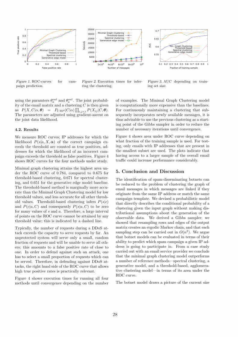
Finding Botnets Using Minimal Graph Clusterings
0
0.2
0.4
0.6
0.8
1
0 0.2 0.4 0.6 0.8 1
Tru
e pos
itiv
e ra
te
False positive rate
Minimal Graph ClusteringThreshold-based
Spectral clusteringGenerative edge model
Figure 1. ROC-curves for cam-paign prediction.
0
5000
10000
15000
20000
25000
30000
35000
2x10⁴ 4x10⁴ 6x10⁴ 8x10⁴ 105
Sec
onds
Number of messages
Minimal Graph ClusteringThreshold-based
Spectral clusteringGenerative edge model
Figure 2. Execution times for infer-ring the clustering.
0.55
0.6
0.65
0.7
0.1 0.2 0.3 0.4 0.5 0.6 0.7 0.8 0.9 1
AU
C
Fraction of training sample
Min. Graph ClusteringThreshold-based
Spectral clusteringGenerative edge model
Figure 3. AUC depending on train-ing set size.
using the paramters θouta and θouta . The joint probabil-ity of the email matrix and a clustering C is then givenas P (X,C|α,θ) = PCRP (C|α)
∏i,j<i P (Xij |C,θ).
The parameters are adjusted using gradient-ascent onthe joint data likelihood.
4.2. Results
We measure ROC curves; IP addresses for which thelikelihood P (s|a,X,α) of the correct campaign ex-ceeds the threshold are counted as true positives, ad-dresses for which the likelihood of an incorrect cam-paign exceeds the threshold as false positives. Figure 4shows ROC curves for the four methods under study.
Minimal graph clustering attains the highest area un-der the ROC curve of 0.784, compared to 0.675 forthreshold-based clustering, 0.671 for spectral cluster-ing, and 0.651 for the generative edge model baseline.The threshold-based method is marginally more accu-rate than the Minimal Graph Clustering model for lowthreshold values, and less accurate for all other thresh-old values. Threshold-based clustering infers P (s|c)and P (c|a,C) and consequently P (s|a,C) to be zerofor many values of s and a. Therefore, a large intervalof points on the ROC curve cannot be attained by anythreshold value; this is indicated by a dashed line.
Typically, the number of requests during a DDoS at-tack exceeds the capacity to serve requests by far. Anunprotected system will serve only a small, randomfraction of requests and will be unable to serve all oth-ers; this amounts to a false positive rate of close toone. In order to defend against such an attack, onehas to select a small proportion of requests which canbe served. Therefore, in defending against DDoS at-tacks, the right hand side of the ROC curve that allowshigh true positive rates is practically relevant.
Figure 4 shows execution times for running all fourmethods until convergence depending on the number
of examples. The Minimal Graph Clustering modelis computationally more expensive than the baselines.For continuously maintaining a clustering that sub-sequently incorporates newly available messages, it isthus advisable to use the previous clustering as a start-ing point of the Gibbs sampler in order to reduce thenumber of necessary iterations until convergence.
Figure 4 shows area under ROC curve depending onwhat fraction of the training sample is used. For test-ing, only emails with IP addresses that are present inthe smallest subset are used. The plots indicate thathaving access to a larger sample of the overall emailtraffic could increase performance considerably.
5. Conclusion and Discussion
The identification of spam-disseminating botnets canbe reduced to the problem of clustering the graph ofemail messages in which messages are linked if theyoriginate from the same IP address or match the samecampaign template. We devised a probabilistic modelthat directly describes the conditional probability of aclustering given the input graph without making dis-tributional assumptions about the generation of theobservable data. We derived a Gibbs sampler; weshowed that resampling rows and edges of the outputmatrix creates an ergodic Markov chain, and that eachsampling step can be carried out in O(n2). We arguethat botnet models can be evaluated in terms of theirability to predict which spam campaign a given IP ad-dress is going to participate in. From a case studycarried out with an email service provider we concludethat the minimal graph clustering model outperformsa number of reference methods—spectral clustering, agenerative model, and a threshold-based, agglomera-tive clustering model—in terms of its area under theROC curve.
The botnet model draws a picture of the current size
28

Finding Botnets Using Minimal Graph Clusterings
and activity of botnets. From the IP addresses, the ge-ographical distribution of each botnet can be derived.The botnet model can be used to select particularlyprolific botnets for in-depth analysis and possible le-gal action. Widespread botnet software is versatileand supports both, dissemination of email spam andthe staging of network attacks (Stern, 2008). Whenboth, a mailing campaign and a network attack arecarried out by a single network within the typical IP-address reassignment interval of one day, then thebotnet model which has been trained on email datacan score HTTP requests by the likelihood that theirsender IP address is part of an attacking botnet. Thisallows to prioritize requests and to maintain a serviceduring an attack. Alternatively, the botnet model canbe trained with HTTP requests instead of emails; therecipient domain of an HTTP request plays the roleof the campaign template. Again, the botnet modelallows to infer the likelihood that an individual senderIP address acts as part of an attacking botnet.
Direct evaluation of the model’s ability to decidewhether an IP request is part of a network attackwould require evaluation data in the form of a col-lection of individual HTTP requests labeled with thebotnet that has sent the request. While it is relativelyeasy to collect the entire stream of legitimate and at-tacking HTTP requests that reach a domain duringan attack, there is no practical means of labeling indi-vidual requests. In general, HTTP requests contain noinformation that allows even a human expert to decidewhether a request is part of an attack, let alone whichbotnet a request has really been sent from.
6. Acknowledgments
This work was funded by a grant from STRATO AG.
References
Chen, Wen-Yen, Song, Yangqiu, Bai, Hongjie, Lin, Chih-Jen, and Chang, Edward Y. Parallel spectral clusteringin distributed systems. IEEE Transactions on PatternAnalysis and Machine Intelligence, 33(3):568–586, 2011.
Choi, H., Lee, H., and Kim, H. Botgad: detecting botnetsby capturing group activities in network traffic. In Pro-ceedings of the Fourth International ICST Conferenceon COMmunication System softWAre and middlewaRE,pp. 2. ACM, 2009.
DiBenedetto, S., Gadkari, K., Diel, N., Steiner, A., Massey,D., and Papadopoulos, C. Fingerprinting custom botnetprotocol stacks. In Secure Network Protocols (NPSec),2010 6th IEEE Workshop on, pp. 61–66. IEEE, 2010.
Dittrich, D. and Dietrich, S. Discovery techniques for p2pbotnets, 2008.
Goebel, J. and Holz, T. Rishi: Identify bot contaminatedhosts by irc nickname evaluation. In Proceedings of thefirst conference on First Workshop on Hot Topics inUnderstanding Botnets, pp. 8–8. USENIX Association,2007.
Gu, G., Perdisci, R., Zhang, J., and Lee, W. Botminer:Clustering analysis of network traffic for protocol-andstructure-independent botnet detection. In Proceedingsof the 17th conference on Security symposium, pp. 139–154. USENIX Association, 2008.
Haider, P. and Scheffer, T. Bayesian clustering for emailcampaign detection. In Proceeding of the InternationalConference on Machine Learning, 2009.
Hammersley, J. and Clifford, P. Markov fields on finitegraphs and lattices, 1971.
Holz, T., Steiner, M., Frederic, D., Biersack, E., and Freil-ing, F. Measurements and mitigation of peer-to-peer-based botnets: a case study on storm worm. In Proceed-ings of the USENIX Workshop on Large-Scale Exploitsand Emergent Threats, 2008.
John, J.P., Moshchuk, A., Gribble, S.D., and Krishna-murthy, A. Studying spamming botnets using botlab.In Proceedings of the 6th USENIX symposium on Net-worked systems design and implementation, pp. 291–306.USENIX Association, 2009.
Mori, T., Esquivel, H., Akella, A., Shimoda, A., and Goto,S. Understanding large-scale spamming botnets frominternet edge sites. In Proceedings of the Conference onE-Mail and Anti-Spam. CEAS, 2010.
Pitman, J. and Picard, J. Combinatorial stochastic pro-cesses. Springer, 2006. ISBN 354030990X.
Stern, H. A survey of modern spam tools. In Proceedingsof the Conference on Email and Anti-Spam, 2008.
Xie, Y., Yu, F., Achan, K., Panigrahy, R., Hulten, G., andOsipkov, I. Spamming botnets: Signatures and charac-teristics. ACM SIGCOMM Computer CommunicationReview, 38(4):171–182, 2008.
Yu, F., Xie, Y., and Ke, Q. Sbotminer: Large scale searchbot detection. In Proceedings of the third ACM interna-tional conference on Web search and data mining, pp.421–430. ACM, 2010.
Zhuang, L., Dunagan, J., Simon, D.R., Wang, H.J., andTygar, JD. Characterizing botnets from email spamrecords. In Proceedings of the 1st Usenix Workshopon Large-Scale Exploits and Emergent Threats, pp. 1–9. USENIX Association, 2008.
29

Learning from Incomplete Data with Infinite Imputations
Uwe Dick [email protected] Haider [email protected] Scheffer [email protected]
Max Planck Institute for Computer Science, Saarbrucken, Germany
Abstract
We address the problem of learning deci-sion functions from training data in whichsome attribute values are unobserved. Thisproblem can arise, for instance, when train-ing data is aggregated from multiple sources,and some sources record only a subset of at-tributes. We derive a generic joint optimiza-tion problem in which the distribution gov-erning the missing values is a free parame-ter. We show that the optimal solution con-centrates the density mass on finitely manyimputations, and provide a corresponding al-gorithm for learning from incomplete data.We report on empirical results on benchmarkdata, and on the email spam application thatmotivates our work.
1. Introduction
In many applications, one has to deal with trainingdata with incompletely observed attributes. For in-stance, training data may be aggregated from differ-ent sources. If not all sources are capable of providingthe same set of input attributes, the combined train-ing sample contains incompletely observed data. Thissituation occurs in email spam detection, where it ishelpful to augment the content of an email with real-time information about the sending server, such as itsblacklist status. This information is available for alltraining emails that arrive at a mail server under one’sown control, and it is also available at application time.But if one wants to utilize training emails from publicarchives, this information is missing.
We adress a learning setting in which values are miss-ing at random: here, the presence or absence of values
Appearing in Proceedings of the 25 th International Confer-ence on Machine Learning, Helsinki, Finland, 2008. Copy-right 2008 by the author(s)/owner(s).
does not convey information about the class labels. Ifthis condition is not met, it is informative to considerthe presence or absence of values as additional input tothe decision function. Techniques for learning from in-complete data typically involve a distributional modelthat imputes missing values, and the desired final pre-dictive model. Prior work on learning from incompletedata is manifold in the literature, and may be groupedby the way the distributional model is used.
The first group models the distribution of missing val-ues in a first step, and learns the decision functionbased on the distributional model in a second step.Shivaswamy et al. (2006) formulate a loss functionthat takes a fixed proportion of the probability massof each instance into account, with respect to the es-timated distribution of missing values. They derivesecond order cone programs which renders the methodapplicable only to very small problems. Other exam-ples include Williams and Carin (2005), Williams et al.(2005), and Smola et al. (2005).
The second group estimates the parameters of a distri-butional model and the final predictive model jointly.As an example, recently Liao et al. (2007) proposean EM-algorithm for jointly estimating the imputa-tion model and a logistic regression classifier with lin-ear kernel, assuming the data arises from a mixture ofmultivariate Gaussians.
The third group makes no model assumption about themissing values, but learns the decision function basedon the visible input alone. For example, Chechik et al.(2007) derive a geometrically motivated approach. Foreach example, the margin is re-scaled according to thevisible attributes. This procedure specifically aims atlearning from data with values that are structurallymissing—as opposed to missing at random. Chechiket al. (2007) find empirically that the procedure is notadequate when values are missing at random.
Jointly learning a distributional model and a kernelpredictive model relates to the problem of learning a
30

Learning from Incomplete Data with Infinite Imputations
kernel function from a prescribed set of parameterizedkernels. This problen drew a lot of attention recently;see, for example, Argyriou et al. (2005) and Micchelliand Pontil (2007).
Estimating the distributional model first and trainingthe predictive model in a second step leaves the userfree to choose any learning algorithm for this secondstep. However, a harder problem has to be solved thanwould be necessary. If one is only interested in a deci-sion function that minimizes the desired loss, knowingthe values or distribution of the missing attributes inthe training set is not actually required. Furthermore,errors made in the imputation step and errors made inestimating the parameters of the predictive model canadd up in a sequential procedure.
Consequently, we investigate learning the decisionfunction and the distribution of imputations depen-dently. Unlike prior work on this topic, we develop asolution for a very general class of optimization crite-ria. Our solution covers a wide range of loss functionsfor classification and regression problems. It comeswith all the usual benefits of kernel methods. We de-rive an optimization problem in which the distributiongoverning the missing values is a free parameter. Theoptimization problem searches for a decision functionand a distribution governing the missing values whichtogether minimize a regularized empirical risk.
No fixed parametric form of the distributional modelis assumed. A regularizer that can be motivated by adistributional assumption may bias the distributionalmodel towards a prior belief. However, the regularizermay be overruled by the data, and the resulting distri-butional model may be different from any parametricform. We are able to prove that there exists an opti-mal solution based on a distribution that is supportedby finitely many imputations. This justifies a greedyalgorithm for finding a solution. We derive manifesta-tions of the general learning method and study themempirically.
The paper is structured as follows. After introducingthe problem setting in Section 2, we derive an opti-mization problem in Section 3. Section 4 proves thatthere is an optimal solution that concentrates the den-sity mass on finitely many imputations and presentsan algorithm. Example instantiations of the generalsolution are presented in Section 5. We empiricallyevaluate the method in Section 6. Section 7 concludes.
2. Problem Setting
We address the problem of learning a decision func-tion f from a training sample in which some attribute
values are unobserved.
Let X be a matrix of n training instances xi and lety be the vector of corresponding target values yi. In-stances and target values are drawn iid from an un-known distribution p(x, y) with xi ∈ Rd and yi ∈ Y,where Y denotes the set of possible target values. Ma-trix Z indicates which features are observed. A valueof zil = 1 indicates that xil, the l-th feature of the i-thexample, is observed. Values are missing at random:yi is conditionally independent of zi given xi.
The goal is to learn a function f : x 7→ y that pre-dicts target values for completely observed examples.The decision function should incur only a minimal truerisk R(f) =
∫L(y, f(x))p(x, y)dxdy, where L is a loss
function for the task at hand.
As a means to minimizing the true risk, we seek afunction f in the reproducing kernel Hilbert space Hk
induced by a kernel k that minimizes a regularizedempirical risk functional R(f) =
∑ni=1 l(yi, f(xi)) +
η‖f‖2k. We demand k to be a Mercer kernel. Lossfunction l approximates the true loss L. The represen-ter theorem allows us to write the minimizer as a sumover functions in Hk centered at training instances:f(x) =
∑nj=1 cjk(xj ,x).
The learning problem from completely observed datawould amount to solving Optimization Problem 1.
Optimization Problem 1 (Primal learning prob-lem, observed data). Over c, minimize
R(c, k)=n∑
i=1
l(yi,
n∑
j=1
cjk(xj ,xi))+η
n∑
i,j=1
cicjk(xj ,xi)
We require that the loss function be defined in sucha way that Optimization Problem 1 can be writtenin the dual form of Optimization Problem 2. A widerange of loss functions satisfies this demand; we willlater see that this includes hinge loss and squared loss.
Optimization Problem 2 (Dual of learningproblem). Given a < 0, over c, maximize
a 〈c,Kc〉 −R∗(c)
subject to the constraints
∀m∗1
i=1g∗i (c) ≤ 0, ∀m
∗2
j=1h∗j (c) = 0. (1)
R∗(c) denotes a differentiable convex function of thedual variables c which we demand to be independentof the kernel matrix K. The inequality constraints g∗iare differentiable convex and the equality constraintsh∗j differentiable affine. We like to note that the re-
quirement of independence between R∗ and K is not
31

Learning from Incomplete Data with Infinite Imputations
very restrictive in practice, as we will see in chapter5. Furthermore, we demand strong duality to holdbetween Optimization problems 1 and 2.
3. Learning from Incomplete Data inOne Step
If any instance xi has unobserved features, thenk(xi,x) and, consequently, the decision function f arenot properly defined. In order to learn from incom-plete data, we will marginalize the decision functionand risk functional by the observable attributes andintegrate over all unobserved quantities. To this end,we define ω ∈ ΩZ
X ⊂ Rn×d as a matrix of imputationsconstrained by ωil = xil if zil = 1. We demand ΩZ
X tobe compact for the rest of this paper. Let ωi denotethe i-th row of ω. Then we can define a family of ker-nels K(ω)(xj ,xi) = k(ωj ,ωi). Any probability mea-sure p(ω) on imputations induces a marginalization ofthe kernel by the observable variables. Equation 2 in-tegrates over all imputations of unobserved values; itcan be evaluated based on the observed values.
K(p)(xj ,xi) =
∫
ω∈ΩZX
k(ωj ,ωi)dp(ω) (2)
Any probability measure p(ω) constitutes an optimiza-tion criterion R(c,K(p)). In the absence of knowledgeabout the true distribution of missing values, p(ω) be-comes a free parameter. Note that p(ω) is a continu-ous probability measure that is not constrained to anyparticular parametric form; the space of parameters istherefore of infinite dimensionality.
It is natural to add a regularizer Q(p) that reflectsprior belief on the distribution of imputations p(ω) tothe optimization criterion, in addition to the empiri-cal risk and regularizer on the predictive model. Theregularizer is assumed to be continuous in p. The reg-ularizer does not constrain p(ω) to any specific classof distribution, but it reflects that some distributionsare believed to be more likely. Without a regularizer,the criterion can often be minimized by imputationswhich move instances with missing values far awayfrom the separator, thereby removing their influenceon the outcome of the learning process. This leads toOptimization Problem 3.
Optimization Problem 3 (Learning problemwith infinite imputations). Given n training ex-amples with incomplete feature values, γ > 0, kernelfunction k, over all c and p, minimize
Rk,γ(c, p) = R(c,K(p)) + γQ(p) (3)
subject to the constraints
∀ω : p(ω) ≥ 0,∫ω∈ΩZ
Xp(ω)dω = 1.
Each solution to Optimization Problem 3 integratesover infinitely many different imputations. The searchspace contains all continuous probability measures onimputations, the search is guided by the regularizer Q.The regularization parameter γ determines the influ-ence of the regularization on the resulting distribution.For γ → ∞ the solution of the optimization reducesto the solution obtained by first estimating the distri-bution of missing attribute values that minimizes theregularizer. For γ → 0 the solution is constituted bythe distribution minimizing the risk functional R.
4. Solving the Optimization Problem
In this section, we devise a method for efficiently find-ing a solution to Optimization Problem 3. Firstly, weshow that there exists an optimal solution c, p with psupported on at most n+2 imputations ω ∈ ΩZ
X. Sec-ondly, we present an algorithm that iteratively findsthe optimal imputations and parameters minimizingthe regularized empirical risk.
4.1. Optimal Solution with Finite Combination
In addition to the parameters c of the predictive mod-els, continuous probability measure p(ω) contributesan infinite set of parameters to Optimization Problem3. The implementation of imputations as parametersof a kernel family allows us to show that there existsan optimal probability measure p for Equation 3 suchthat p consists of finitely many different imputations.
Theorem 1. Optimization Problem 3 has an optimalsolution c, p in which p is supported by at most n + 2imputations ω ∈ ΩZ
X.
Proof. The compactness of ΩZX and the continuity ofK
immediately imply that there exists some solution toOptimization Problem 3. It remains to be shown thatat least one of the solutions is supported by at mostn+ 2 imputations. Let c, p be any solution and let allrequirements of the previous section hold. The ideaof this proof is to construct a correspondence betweendistributions over imputations and vectors in Rn+1,where a finite support set is known to exist. DefineS(ω) = K(ω)c ∈ Rn and D = (S(ω)⊤, Q(ω))⊤ : ω ∈ΩZ
X ⊂ Rn+1. Since ΩZX is compact and K(·) and Q(·)
are continuous by definition, D is compact as well. Wedefine a measure over D as µ(A×B) = p(ω : S(ω) ∈A ∧Q(ω) ∈ B).Then, by Caratheodory’s convex hull theorem, thereexists a set of k vectors (s⊤1 , q1)⊤, . . . , (s⊤k , qk)⊤ ⊆ Dwith k ≤ n + 2 and nonnegative constants νi with
32

Learning from Incomplete Data with Infinite Imputations
∑ki=1 νi = 1, such that
∫
D
(s⊤, q)⊤dµ((s⊤, q)⊤) =k∑
i=1
(s⊤i , qi)⊤νi.
For each i, select any ωi such that (S(ωi)⊤, Q(ωi)) =
(s⊤i , qi). We construct p by setting p(ω) =∑k
i=1 νiδωi,
where δωidenotes the Dirac measure at ωi. The op-
timal c results as argminc R(c,K(p)). We have
∫
D
sdµ((s⊤, q)⊤) =
k∑
i=1
siνi, and
∫
D
qdµ((s⊤, q)⊤) =
k∑
i=1
qiνi.
Then
K(p)c =
(∫
ΩZX
K(ω)dp(ω)
)c =
∫
ΩZX
S(ω)dp(ω)
=
∫
D
S(ω)dµ((S(ω)⊤, Q(ω))⊤
)
=
k∑
i=1
siνi =
∫
ΩZX
S(ω)dp(ω)
=
∫
ΩZX
K(ω)dp(ω)c = K(p)c.
Likewise,
Q (p) =
∫
D
Q (ω) dµ((S(ω)⊤, Q(ω))⊤
)
=
k∑
i=1
qiνi = Q(p).
Since Q(p) does not depend on c, c =argminc R(c,K(p)), and by strong duality,c = argmaxc a 〈c,K(p)c〉 − R∗(c). This impliesthat the Karush-Kuhn-Tucker conditions hold for c,namely there exist constants κi ≥ 0 and λj such that
aK(p)c−∇R∗(c) +∑
i
κi∇g∗i (c) +∑
j
λj∇h∗j (c) = 0
∀i g∗i (c) ≤ 0, ∀j h∗i (c) = 0, ∀i κig
∗i (c) = 0
It is easy to see that therefore c is also a maximizerof a 〈c,K(p)c〉 − R∗(c), because K(p)c = K(p)c andthe Karush-Kuhn-Tucker conditions still hold. Theirsufficiency follows from the fact that K(p) is positivesemi-definite for any p, and the convexity and affinitypremises. Thus,
R(c,K(p)) + γQ(p)
=[minc
R(c,K(p))]+ γQ(p)
=[max
ca 〈c,K(p)c〉 −R∗(c)
]+ γQ(p)
= [a 〈c,K(p)c〉 −R∗(c)] + γQ(p)
= [a 〈c,K(p)c〉 −R∗(c)] + γQ(p)
=[max
ca 〈c,K(p)c〉 −R∗(c)
]+ γQ(p)
=[minc
R(c,K(p))]+ γQ(p)
= R(c,K(p)) + γQ(p).
We have now established that there exists a solutionwith at most n+ 2 imputations.
4.2. Iterative Optimization Algorithm
This result justifies the following greedy algorithm tofind an optimal solution to Optimization Problem 3.The algorithm works by iteratively optimizing Prob-lem 1 (or, equivalently, 2), and updating the distribu-tion over the missing attribute values. Let pω denotethe distribution p(ω) = δω. Algorithm 1 shows thesteps.
Algorithm 1 Compute optimal distribution of impu-tations on ΩZ
X
Initialization: Choose p(1) = pω(1) ; e.g., ω(1)il = 0 for
all zil 6= 1for t = 1 . . . do1. c← argminc R(c,K(p(t)))2. Find ω(t+1) ∈ ΩZ
X : Rk,γ(c, pω(t+1)) <
Rk,γ(c, p(t)). If no such ω(t+1) exists, terminate.
3. βt ← argminβ∈(0,1]
[minc Rk,γ(c, βpω(t+1) +
(1− β)p(t))]
4. p(t+1) ← βtpω(t+1) + (1− βt)p(t)
5. ∀j < t : βj ← βj(1− βt)end for
Step 1 consists of minimizing the regularized empiri-cal risk functional R, given the current distribution.In step 2 a new imputation is constructed which im-proves on the current objective value. Since in gen-eral Rk,γ(c, pω) is not convex in ω, one cannot findthe optimal ω efficiently. But the algorithm only re-quires to find any better ω. Thus it is reasonable toperform gradient ascent on ω, with random restartsin case the found local optimum does not satisfy theinequality of step 2. In step 3 and 4 the optimal dis-tribution consisting of the weighted sum of currentlyused Dirac impulses
∑ti=1 βiδωi
and the new imputa-tion δω(t+1) is computed. This step is convex in β if
33

Learning from Incomplete Data with Infinite Imputations
Rk,γ(c, βpω(t+1) +(1−β)p(t)) is linear in β. By lookingat Optimization Problem 2, we see that this is the casefor R. Thus the convexity depends on the choice forQ (see Sect. 5.2). Step 5 updates the weights of theprevious imputations.
The algorithm finds t imputations ω(j) and theirweights βj , as well as the optimal example coefficientsc. We can construct the classification function f as
f(x) =t∑
j=1
n∑
i=1
βjcik(ω(j)i ,x). (4)
Note that the value n + 2 is an upper bound for thenumber of basic kernels which constitute the optimalsolution. The algorithm is not guaranteed to terminateafter n + 2 iterations, because the calculated imputa-tions are not necessarily optimal. In practice, however,the number of iterations is usually much lower. In ourexperiments, the objective value of the optimizationproblem converges in less than 50 iterations.
5. Example Learners
In this chapter we present manifestations of the genericmethod, which we call weighted infinite imputations,for learning from incomplete data that we use in theexperimental evaluation.
Recall from Section 3 the goal to learn a decision func-tion f from incomplete data that minimizes the ex-pected risk R(f) =
∫L(y, f(x))p(x, y)dxdy. In clas-
sification problems the natural loss function L be-comes the zero-one loss, whereas in regression prob-lems the loss depends on the specific application; com-mon choices are the squared error or the ǫ-insensitiveloss. The considerations in the previous chapters showthat, in order to learn regression or classification func-tions from training instances with missing attributevalues, we only have to specify the dual formulation ofthe preferred learning algorithm on complete data anda regularizer on the distribution of imputations p.
5.1. Two Standard Learning Algorithms
For binary classification problems, we choose to ap-proximate the zero-one by the hinge loss and performsupport vector machine learning. The dual formula-tion of the SVM is given by RSVM (c, k) =
∑ni=1
ciyi−
12
∑ni,j=1 cicjk(xj ,xi) subject to the constraints 0 ≤
ciyi≤ 1
η and∑n
i=1 ci = 0. We see that the demandsof Optimization Problem 2 are met and a finite solu-tion can be found. Taking the SVM formulation asthe dual Optimization Problem 2 gives us the means –in conjunction with an appropriate regularizer Q – to
learn a classification function f from incomplete data.
For regression problems, the loss depends on the taskat hand, as noted above. We focus on penalizing thesquared error, though we like to mention that the ap-proach works for other losses likewise. One widely usedlearning algorithm for solving the problem is kernelridge regression. Again, we can learn the regressionfunction f from incomplete data by using the sameprinciples as described above. Kernel ridge regressionminimizes the regularized empirical risk
∑ni=1(yi −
f(xi))2 + η‖f‖2. The dual formulation RKRR(c, k) =∑n
i=1 ciyi − 14
∑ni=1 c
2i + 1
4η
∑ni,j=1 cicjk(xi, xj) again
meets the demands of the dual optimization problem2. Substituting its primal formulation for R in step 1of Algorithm 1 and in Eqn. 3 solves the problem oflearning the regression function from incomplete dataafter specifying a regularizer Q.
5.2. Regularizing towards Prior Belief inFeature Space
A regularizer on the distribution of missing values canguide the search towards distributions ω that we be-lieve to be likely. We introduce a regularization termwhich penalizes imputations that are different fromour prior belief ω. We choose to penalize the sumof squared distances between instances xi and ωi infeature space Hk induced by kernel k. We define thesquared distance regularization term Qsq as
Qsq(k, ω) =
n∑
i=1
‖φk(xi)− φk(ωi)‖22
=n∑
i=1
k(xi,xi)− 2k(xi, ωi) + k(ωi, ωi).
Note that when using Qsq, step 3 of Algorithm 1 be-comes a convex minimization procedure.
5.3. Imputing the Mean in Feature Space
In principle any imputation we believe is useful forlearning a good classifier can be used as ω. Sev-eral models of the data can be assumed to com-pute corresponding optimal imputations. We liketo mention one interesting model, namely the class-based mean imputation in the feature space Hk in-duced by kernel k. This model imputes missingvalues such that the sum of squared distances be-tween completed instances to the class-dependentmean in feature space is minimal over all possi-ble imputations. ω = argminω
∑ni=1 ‖φk(ωi) −
1nyi
∑j:yj=yi
φk(ωj)‖22, where ny denotes the num-
ber of instances with label y. Simple alge-braic manipulations show that this is equivalent to
34

Learning from Incomplete Data with Infinite Imputations
minimizing the sum of squared distances betweenall instances
∑υ∈−1,1
1nυ
∑i,j:yi=yj=υ ‖φk(ωi) −
φk(ωj)‖22 =∑
υ∈−1,11nυ
∑i,j:yi=yj=υ
[k(ωi,ωi) −
2k(ωi,ωj) + k(ωj ,ωj)]
Definition 1 (Mean in Feature Space). The class-based mean in feature space imputation method im-putes missing values ω which optimize
ω = argminω
∑
υ∈−1,+1
1
nυ
∑
i,j:yi=yj=υ[k(ωi,ωi)− 2k(ωi,ωj) + k(ωj ,ωj)
]
Note that this model reduces to the standard mean ininput space when using the linear kernel.
6. Empirical Evaluation
We evaluate the performance of our generic approachweighted infinite imputations for two example realiza-tions. We test for classification performance on theemail spam data set which motivates our investiga-tion. Furthermore, we test on seven additional binaryclassification problems and three regression problems.
6.1. Classification
We choose to learn the decision function for the binaryclassification task by substituting the risk functional ofthe support vector machine, −RSVM , as presented insection 5.1 for R and the squared distance regularizerQsq (Section 5.2) for Q in Optimization Problem 3.
For the motivating problem setting, we assemble adata set of 2509 spam and non-spam emails, whichare preprocessed by a linear text classifier which iscurrently in use at a large webspace hosting company.This classifier discriminates reasonably well betweenspam and non-spam, but there is still a small fractionof misclassified emails. The classifier has been trainedon about 1 million emails from a variety of sources, in-cluding spam-traps as well as emails from the hostingcompany itself, recognizing more than 10 million dis-tinct text features. On this scale, training a supportvector machine with Gaussian kernel is impractical,therefore we employ a two-step procedure. We discardthe contents of the emails and retain only their spamscore from the text classifier and their size in bytes ascontent features in the second-step classifier. At thetime of collection of the emails, we record auxiliaryreal-time information about the sending servers. Thisincludes the number of valid and invalid receiver ad-dresses of all emails seen from the server so far, andthe mean and standard deviation of the sizes and spamscores of all emails from the server. Such information
is not available for emails from external sources, butwill be available when classifying unseen emails. Werandomly draw 1259 emails, both spam and non-spam,with server information, whereas half of those weredrawn from a set of misclassified spam-emails. We aug-ment this set with 1250 emails drawn randomly froma source without server information for which only 2of the 8 attributes are observed.
To evaluate the common odd versus even digits dis-crimination, random subsets of 1000 training examplesfrom the USPS handwritten digit recognition set areused. We test on the remaining 6291 examples. Ad-ditionally, we test on KDD Cup 2004 Physics (1000train, 5179 test, 78 attributes) data set and on the4-view land mine detection data (500, 213, 41) asused by Williams and Carin (2005). In the latter,instances consist of 4 views on the data, each froma separate sensor. Consequently, we randomly selectcomplete views as missing. From the UCI machinelearning repository we take the Breast (277 instances,9 features), Diabetes (768, 8), German (1000, 20), andWaveform (5000, 21) data sets. Selection criteria forthis subset of the repository were minimum require-ments on sample size and number of attributes.
On each data set we test the performance of weightedinfinite imputation using four different regularizationimputations ω for the regularizer Qsq(K(p), ω). Theseimputations are computed by mean imputation in in-put space (MeanInput) and mean imputation in fea-ture space (MeanFeat) as by Definition 1. Addi-tionally we use the EM algorithm to compute the at-tributes imputed by the maximum likelihood parame-ters of an assumed multivariate Gaussian distributionwith no restrictions on the covariate matrix (Gauss),and a Gaussian Mixture Model with 10 Gauss centersand spherical covariances (GMM).
Four learning procedures based on single imputationsserve as reference methods: the MeanInput, Mean-Feat, Gauss, and GMM reference methods first de-termine a single imputation, and then invoke the learn-ing algorithm.
All experiments use a spheric Gaussian kernel. Its vari-ance parameter σ as well as the SVM-parameter η areadjusted using the regular SVM with a training andtest split on fully observed data. All experiments onthe same data set use this resulting parameter setting.Results are averaged over 100 runs were in each runtraining and test split as well as missing attributes arechosen randomly. If not stated otherwise, 85% of at-tributes are marked missing on all data sets. In orderto evaluate our method on the email data set, we per-form 20-fold cross-validation. Since the emails with
35

Learning from Incomplete Data with Infinite Imputations
Table 1. Classification accuracies and standard errors for all data sets. Higher accuracy values are written in bold face,“∗” denotes significant classification improvement.
MeanInput Gauss GMM MeanFeat
Email Single imp 0.9571± 0.0022 0.9412± 0.0037 0.9505± 0.0030 0.9570± 0.0022WII 0.9571± 0.0022 0.9536± 0.0022 ∗ 0.9527± 0.0024 0.9600± 0.0019 ∗
USPS Single imp 0.8581± 0.0027 0.8688± 0.0022 0.9063± 0.0012 0.8581± 0.0027WII 0.8641± 0.0027 ∗ 0.8824± 0.0024 ∗ 0.9105± 0.0015 ∗ 0.8687± 0.0027 ∗
Physics Single imp 0.6957± 0.0035 0.5575± 0.0038 0.6137± 0.0050 0.6935± 0.0028WII 0.7084± 0.0039 ∗ 0.6543± 0.0055 ∗ 0.6881± 0.0049 ∗ 0.7036± 0.0032 ∗
Mine Single imp 0.8650± 0.0025 0.8887± 0.0023 0.8916± 0.0023 0.8660± 0.0026WII 0.8833± 0.0026 ∗ 0.8921± 0.0021 0.8946± 0.0022 ∗ 0.8844± 0.0026 ∗
Breast Single imp 0.7170± 0.0055 0.7200± 0.0048 0.7164± 0.0048 0.7085± 0.0057WII 0.7184± 0.0056 0.7243± 0.0048 ∗ 0.7212± 0.0050 ∗ 0.7152± 0.0057 ∗
Diabetes Single imp 0.7448± 0.0025 0.7053± 0.0036 0.7154± 0.0043 0.7438± 0.0026WII 0.7455± 0.0025 0.7234± 0.0036 ∗ 0.7389± 0.0031 ∗ 0.7439± 0.0024
German Single imp 0.7331± 0.0029 0.7058± 0.0029 0.7056± 0.0028 0.7364± 0.0029WII 0.7368± 0.0025 ∗ 0.7118± 0.0030 ∗ 0.7120± 0.0028 ∗ 0.7357± 0.0027
Waveform Single imp 0.8700± 0.0019 0.8241± 0.0031 0.7827± 0.0049 0.8679± 0.0020WII 0.8700± 0.0019 0.8612± 0.0019 ∗ 0.8583± 0.0020 ∗ 0.8686± 0.0020 ∗
-0.01
0
0.01
0.02
0.03
0.04
0.05
0.06
0.07
0.08
10 20 30 40 50 60 70 80 90
Acc
urac
y
% Missing
1. Improvement by % Missing
MeanInputGaussGMM
MeanFeat
0
0.01
0.02
0.03
0.04
0.05
200 400 600 800 1000 1200 1400
Acc
urac
y
Size
2. Improvement by Sample Size
MeanInputGaussGMM
MeanFeat
0
2000
4000
6000
8000
10000
12000
14000
16000
500 1500 2500 3500
Tim
e in
sec
onds
Size
3. Execution Time by Sample Size
WII(x/35)2
Figure 1. Detailed results on USPS classification task.
missing attributes cannot be used as test examples,the test sets are only taken from the fully observedpart of the data set.
Table 6.1 shows accuracies and standard errors forthe weighted infinite imputations (WII) method withsquared distance regularization compared to all singleimputations ω on each data set. Regularization pa-rameter γ is automatically chosen for each run basedon the performance on a separate tuning set. Base-lines are obtained by first imputing ω and learning theclassifier in a second step. The weighted infinite impu-tations method outperforms the single imputation invirtually all settings. We test for significant improve-ments with a paired t-test on the 5% significance level.Significant improvements are marked with a “∗” in thetable.
We explore the dependence of classification perfor-
mance on training sample size and the percentage ofmissing attribute values in more detail. The first graphin Figure 1 shows improvements in classification accu-racy of our method over the single imputations de-pending on the percentage of missing values. Graph2 shows classification accuracy improvements depend-ing on the size of the labeled training set. Both ex-periments are performed on USPS data set and weagain adjust γ separately for each run based on theperformance on the tuning set. We note that similarresults are obtained for the other classification prob-lems. The weighted infinite imputation method canimprove classification accuracy even when only 30%of the attribute values are missing. It shows, though,that it works best if at least 60% are missing, depend-ing on ω. On the other hand, we see that it works forall training set sizes, again depending on ω. Similarresults are obtained for the other data sets.
36

Learning from Incomplete Data with Infinite Imputations
Table 2. Mean squared error results and standard errors for regression data sets. Smaller mean squared errors are writtenin bold face, “∗” denotes significant improvement.
MeanInput Gauss GMM MeanFeat
Housing Single imp 193.0908± 19.9408 288.6192± 41.5954 160.4940± 16.2004 1134.5635± 101.9452WII 66.5144± 0.8958 ∗ 62.3073± 0.8479 ∗ 66.7959± 0.9173 ∗ 64.7926± 0.9619 ∗
Ailerons Single imp 81.7671± 4.5862 172.5037± 8.6705 79.8924± 4.0297 193.5790± 10.4899WII 11.8034± 0.1494 ∗ 8.7505± 0.0932 ∗ 11.7595± 0.1530 ∗ 11.8220± 0.1387 ∗
Cpu act Single imp 10454.176± 962.598 15000.380± 973.100 10123.172± 933.143 15710.812± 1099.603WII 306.257± 12.500 ∗ 204.180± 5.058 ∗ 305.651± 13.627 ∗ 247.988± 8.010 ∗
To evaluate the convergence of our method, we mea-sure classification accuracy after each iteration of thelearning algorithm. It shows that classification accu-racy does not change significantly after about 5 itera-tions for a typical γ, in this case γ = 105 for the USPSdata set. On average the algorithm terminates afterabout 30-40 iterations. The computational demands ofthe weighted infinite imputation method are approxi-mately quadratic in the training set size for the classifi-cation task, as can be seen in Graph 3 of Figure 1. Thisresult depends on the specific risk functional R and itsoptimization implementation. Nevertheless, it showsthat risk functionals which are solvable in quadratictime do not change their computational complexityclass when learned with incomplete data.
6.2. Regression
We evaluate the weighted infinite imputations methodon regression problems using the squared error as lossfunction. Consequently, risk functional RKRR (Sect.5.1) is used as R and again the squared distance reg-ularizer Qsq for Q in Optimization Problem 3. FromUCI we take the Housing data (506, 14), and from theWeka homepage cpu act (1500, 21) and ailerons (2000,40). Ridge parameter η and RBF-kernel parameter σwere again chosen such that they lead to best resultson the completely observed data. Regularization pa-rameter γ was chosen based on the performance ona tuning set consisting of 150 examples. Results areshown in Table 2. We can see that our method outper-forms the results obtained with the single imputationssignificantly for all settings.
7. Conclusion
We devised an optimization problem for learning de-cision functions from incomplete data, where the dis-tribution p of the missing attribute values is a freeparameter. The investigated method makes only mi-nor assumptions on the distribution by the means of aregularizer on p that can be chosen freely. By simul-taneously optimizing the function and the distributionof imputations, their dependency is taken into account
properly. We presented a proof that the optimal so-lution for the joint learning problem concentrates thedensity mass of the distribution on finitely many impu-tations. This justifies the presented iterative algorithmthat finds a solution. We showed that instantiationsof the general learning method consistently outperformsingle imputations.
Acknowledgments
We gratefully acknowledge support from STRATORechenzentrum AG.
References
Argyriou, A., Micchelli, C., & Pontil, M. (2005). Learningconvex combinations of continuously parameterized ba-sic kernels. Proceedings of the 18th Conference on Learn-ing Theory.
Chechik, G., Heitz, G., Elidan, G., Abbeel, P., & Koller,D. (2007). Max-margin classification of incomplete data.Advances in Neural Information Processing Systems 19.
Liao, X., Li, H., & Carin, L. (2007). Quadratically gatedmixture of experts for incomplete data classification.Proceedings of the 24th International Conference on Ma-chine learning.
Micchelli, C., & Pontil, M. (2007). Feature space perspec-tives for learning the kernel. Machine Learning, 66.
Shivaswamy, P. K., Bhattacharyya, C., & Smola, A. J.(2006). Second order cone programming approaches forhandling missing and uncertain data. Journal of Ma-chine Learning Research, 7.
Smola, A., Vishwanathan, S., & Hofmann, T. (2005). Ker-nel methods for missing variables. Proceedings of theTenth International Workshop on Artificial Intelligenceand Statistics.
Williams, D., & Carin, L. (2005). Analytical kernel ma-trix completion with incomplete multi-view data. Pro-ceedings of the ICML 2005 Workshop on Learning WithMultiple Views.
Williams, D., Liao, X., Xue, Y., & Carin, L. (2005).Incomplete-data classification using logistic regression.Proceedings of the 22nd International Conference onMachine learning.
37

Discriminative Clustering for Market Segmentation
Peter Haider∗
Dep. of Computer ScienceUniv. of Potsdam, Germany
Luca Chiarandini†
Web Research GroupUniversitat Pompeu Fabra
Barcelona, [email protected]
Ulf BrefeldUniversity of BonnBonn, Germany
ABSTRACTWe study discriminative clustering for market segmentationtasks. The underlying problem setting resembles discrimi-native clustering, however, existing approaches focus on theprediction of univariate cluster labels. By contrast, marketsegments encode complex (future) behavior of the individ-uals which cannot be represented by a single variable. Inthis paper, we generalize discriminative clustering to struc-tured and complex output variables that can be representedas graphical models. We devise two novel methods to jointlylearn the classifier and the clustering using alternating op-timization and collapsed inference, respectively. The twoapproaches jointly learn a discriminative segmentation ofthe input space and a generative output prediction modelfor each segment. We evaluate our methods on segmentinguser navigation sequences from Yahoo! News. The proposedcollapsed algorithm is observed to outperform baseline ap-proaches such as mixture of experts. We showcase exem-plary projections of the resulting segments to display theinterpretability of the solutions.
Categories and Subject DescriptorsI.5.3 [Clustering]: Algorithms
General TermsAlgorithms, Experimentation
KeywordsDiscriminative Clustering, Market Segmentation
1. INTRODUCTIONMarket segmentation reveals divisions in a given market,
where a market refers to a population of interest such as
∗This work was performed during an internship at Yahoo!Research, Barcelona, Spain.†Also Yahoo! Research, Barcelona, Spain.
Permission to make digital or hard copies of all or part of this work forpersonal or classroom use is granted without fee provided that copies arenot made or distributed for profit or commercial advantage and that copiesbear this notice and the full citation on the first page. To copy otherwise, torepublish, to post on servers or to redistribute to lists, requires prior specificpermission and/or a fee.KDD’12, August 12–16, 2012, Beijing, China.Copyright 2012 ACM 978-1-4503-1462-6 /12/08 ...$15.00.
people, customers, or organizations. A market segment is asubset of a market that is characterized by similar demandsand/or needs based on qualities of a given product such asprice or function.
Every segment is required to meet the following criteria.(i) It is homogeneous within the segment, so that individualswithin the same segment exhibit common needs and can betargeted jointly with the same marketing strategy. (ii) It iseasily distinguishable from other segments to guarantee thatdifferent segments have different demands and (iii) serves asa blueprint for distinct targeting strategies. The require-ments are often summarized as homogeneity, identifiability,and interpretability (19).
Besides frequently deployed self-organizing maps (SOMs)(13; 7), market segmentation matches the problem settingof model-based clustering approaches. Clustering techniqueseither minimize the within-cluster similarity (1; 14), maxi-mize the between-cluster similarity (7), or optimize a combi-nation of both (18), and thus aim to produce homogeneousand identifiable solutions. Once segments have been com-puted, new customers need to be assigned to one of thesubgroups to advertise the product accordingly.
Unfortunately, mapping new instances to an existing clus-tering is often difficult in practice. Intuitively, the new cus-tomer should be grouped to the closest segment with respectto some similarity measure. Closeness can for instance becomputed as the distance in feature space to the median orthe nearest member of a segment (11; 4). However, often atthe time of classifying a new instance, not all features areknown. Even using the similarity measure that is used bythe clustering method itself on all features is frequently ob-served to perform surprisingly inaccurate, see e.g., (20) andSection 4. Other difficulties are for instance distribution-based clusterings, such as Expectation Maximization (6),which assign probabilities for cluster-memberships. By do-ing so, customers are probabilistically related to every seg-ment. Converting this soft assignment into a hard assign-ment by taking a maximum a posteriori or winner-takes-alldecision is often suboptimal if the memberships deviate froma point distribution, in which case more than one segmentsare likely candidates (14).
Optimally, the segmentation is therefore learned togetherwith a classifier that discriminatively maps new instancesto clusters; a problem setting which is also known as dis-criminative clustering (5; 20; 24; 8). The idea is to havethe clustering provide the labels for the classifier which istrained in a supervised manner. The joint optimization al-ters the clustering so that the segments can be easily dis-
38

criminated from each other by the classifier. Combining thetwo criteria thus guarantees concise clusterings and accu-rate classifiers. Existing approaches focus on clustering apopulation and predicting a cluster label for a new instance.By contrast, market segmentation is more complex. In mar-ket segmentation tasks, we need to differentiate between thedata that characterizes individuals and the data that charac-terizes their future behavior. The clustering clearly needs totake all available information into account to generate mean-ingful segments. However, the classifier does not have accessto future events and needs to take a decision on the availableinformation such as gender, income, etc. This observationrenders existing approaches to discriminative clustering toorestrictive for market segmentation tasks.
In this paper we generalize discriminative clustering formarket segmentation tasks using the structured predictionframework. We differentiate between attributes of a cus-tomer and her interests/behavior. Attributes are a prioriavailable features of individuals of the population such asgender or income. Her behavior is a collection of interact-ing variables describing a segment. As segments need to beinterpretable, we model the output data as a complex andstructured variable which can be represented as a graphicalmodel. The distinction allows for learning a classifier only onthe attributes, computing the clustering on both attributesand behavior, and finally summarizing the segments only interms of the behavior.
We devise two solutions which are based on the regular-ized empirical risk minimization framework. The first is astraightforward adaptation of mixtures of experts. Classi-fier and clustering are optimized using an alternating strat-egy where we fix one component while optimizing the other.The second solution uses approximations and integrates outparameters of the classifier using collapsed inference for effi-ciency. Both approaches use generative models for the out-put structure and, in contrast to conventional discriminativeclustering approaches, do not involve trade-off parametersfor classification accuracy and cluster consistency (class bal-ance) because the optimization problems are not prone totrivial and degenerate solutions.
Use cases of our methods contain traditional market seg-mentation tasks. Consider for instance a company that aimsat promoting a new product or a hotel chain that intends tolure visitors with special offers. Our methods not only com-pute a meaningful segmentation of the customers but alsoallow for devising appropriate targeting strategies from thegraphical models. Moreover, our method serves as discrim-inative clustering for structured variables, where the task isnot to output a single class/cluster label but the averagestructure for every segment. The differentiation betweenattributes and behavior increases the range of applicationsthat can be addressed. A special – but still novel – case isobtained when attributes and behavior partially overlap.
Empirically, we study our methods on another interestinguse case: Segmenting user navigation sessions on the Webfor displaying segment-specific website layouts. We experi-ment on a large click log from Yahoo! News. The attributedata is assembled from meta-information about the sessionsuch as the timestamp, the referrer domain, and the firstpage request. The behavior consists of subsequent naviga-tion actions given by click sequences. The generative rep-resentation of the behavior data is interpretable and can beeasily transformed into segment-specific layouts.
The remainder of the paper is structured as follows. Sec-tion 2 discusses the relationship of our problem setting withpreviously studied settings and methods. In Section 3 wederive two algorithms to optimize the empirical counterpartof the expected segmented log-likelihood. Section 4 reportson empirical results using a large click log from a commercialnews provider and Section 5 concludes.
2. RELATED WORKMarket segmentation tasks are often solved using neural
networks such as self-organizing maps (13; 7). Kiang et al.(13) for instance extend self-organizing maps to group cus-tomers according to their attitude towards different commu-nications modes. D’Urso and de Giovanni (7) use the natu-ral clustering property of self-organizing maps together withdissimilarity measures which capture temporal structure ofthe data. In general, clustering data with self-organizingmaps and variants thereof inherently implements the homo-geneity assumption of market segmentation. However, clas-sifying new instances into the clustering is often difficult andit is not possible to output generative models to summarizethe resulting clusters. Additionally, the optimization crite-rion of self-organizing maps is highly sensitive to the actualinitialization and usually converges to different local optima.
Related to market segmentation is the task of estimatinga mixture model for observations (6). Introducing selectorvariables encoding probabilistic cluster-memberships, maxi-mizing the log-likelihood by marginalizing over the selectoris usually straightforward. The selector can be modeled in adata-dependent or data-independent fashion but the prob-abilistic nature of the cluster-memberships render a directapplication for market segmentation tasks impossible.
Discriminative clustering simultaneously computes a seg-mentation of the data at hand and a classifier that discrim-inates the resulting clusters well. Existing approaches in-clude projections into lower-dimensional subspaces (5), jointoptimization of max-margin classifiers and clusterings (20;24), the optimization of scatter metrics (21), and the max-imization of an information theoretic criterion to balanceclass separation and classifier complexity (8). Sinkkonenet al. (17) aim to find clusters that are homogeneous inauxiliary data given by additional discrete variables. Theabove mentioned approaches do not predict any output vari-able but focus on the discrete cluster variable. Moreover, inour generalized problem setting, instances are represented asinput-output pairs. The classifier discriminates the clustersgiven only the input, whereas the cluster parameters need toaccurately estimate the outputs of the contained instances.Previous work on discriminative clustering does not split in-stances into two parts. They represent instances as a singleinput which consequently allows the classifiers to access thewhole example at decision time. The same assumption iscommonly being made in market segmentation studies thatinvolve model-based clustering approaches, (9; 16; 22) butprohibits a natural solution for market segmentation tasks.
This problem setting can be seen as an alteration of thesetting which the Mixture of Experts approach (10; 12) aimsto solve, where the behavior y is predicted given the at-tributes x as a mixture model where the mixture componentweights depend again on x. In our case, mixture componentweights have to be always point distributions as demandedby the application. Framing the distribution of y given themixture component as a pure generative model allows us to
39

derive a more efficient algorithm than that of the Mixtureof Experts approach.
Zhao et al. (23) proposed a maximum-margin cluster-ing for multivariate loss functions. Minimizing the complexlosses allows for capturing structural differences that cannotbe expressed in terms of standard misclassification rates.In principle, by defining a loss function that captures thedifferences of two clusterings, one could possibly solve mar-ket segmentation tasks as their approach implicitly favorsclusterings that are easily discriminable. However, the lossfunction cannot be expressed in terms of the contingency ta-ble of the two clusterings, and the decoding problem in theinner loop of the algorithm, that is finding the most violatedconstraint, becomes intractable in practice.
Also related to our problem setting are multi-view clus-tering approaches, where the data is split into two disjointfeature sets, which are sometimes also called views. Bickeland Scheffer (2) present an intertwined Expectation Maxi-mization algorithm to compute the maximum likelihood so-lution for one view using the expectations provided by itspeer view. The two data views are modeled generativelyand the algorithm maximizes the joint marginal likelihood.By contrast, we aim to find a discriminative classifier on theinput view and instead of maximizing the marginal likeli-hood of the output view we seek to maximize the likelihoodconditioned on a hard cluster assignment.
3. DISCRIMINATIVE SEGMENTATIONWe now present our main contribution, the generalization
of discriminative clustering for structured output variablesto solve market segmentation problems. We introduce theproblem setting in the next section and present a straightfor-ward solution in terms of mixtures of experts in Section 3.2.An efficient approximation is devised in Section 3.3 and Sec-tion 3.3.3 discusses scalability issues.
3.1 PreliminariesWe are given a sampleM from a market where individuals
are represented by tuples (x, y) ∈ X ×Y encoding attributesx and behavior y. Attributes x may encompass individualfeatures like gender, income, etc while the expressed historicbehavior is captured by y ∈ Y and represented as a graph-ical model. The behaviors y are governed by a family ofdistributions denoted by P (y|θ) with natural parameter θ.
In our running example on segmenting user navigation onthe Web, attributes x encode meta-information about thesession such as the timestamp, the referrer domain, and thefirst page request and is represented as a feature vector.The behavior y encodes sequences of the subsequent Webnavigation and can for instance be represented as a Markov-chain where nodes correspond to pageviews and connectingedges visualize clicks.
We aim to find an appropriate segmentation of the mar-ket M. Formally, the goal is to find a classifier h : X →1, . . . , k that maps attributes x to one of k clusters, pa-rameterized by θ = (θ1, . . . , θk), where the θj are chosen tomaximize the likelihood of the observed behaviors y of therespective segment. The number of clusters k is assumedto be given by the application at hand, because it consti-tutes a trade-off between predictive power and effort spentfor developing multiple market strategies. As h and θ arenot independent they need to be optimized jointly. Hence,over all classifiers h and parameter collections θ, we aim at
maximizing the expected risk functional R that is defined interms of the segmented log-likelihood
R(h,θ) =
∫logP (y|θh(x))dP (x, y). (1)
Since the true joint distribution P (x, y) is unknown, we re-place Equation (1) by its empirical counterpart on the finitemarket sample of size n given by M = (xi, yi)ni=1
R(θ, h) =
n∑
i=1
logP (yi|θh(xi)). (2)
Directly maximizing Equation (2) in terms of the compo-nent parameters θ and the classifier h is infeasible, since theobjective function is not only highly non-convex and non-continuous but an NP-hard problem because of combinato-rial assignments. However, if the classifier h was fixed, the θjcould be optimized directly, as h provides the segmentationand for each segment j optimal parameters θj are triviallycomputed by
θj = argmaxθ
∑
i:h(xi)=j
logP (yi|θ). (3)
For many common distribution families, the maximum like-lihood estimates P (y|θ) can be computed easily by countingor averaging over the observations in the segment, respec-tively. Vice versa, keeping the segment parameters θ1, . . . , θkfixed, learning the classifier h results in a standard multi-class classification scenario. Using linear models, h can bewritten as
h(x) = argmaxj∈1,...,k
w>j x, (4)
where each segment has its own weight vector wj . In the re-mainder, we will use h and w = (w1, . . . , wk)> interchange-ably. The next section exploits this observation and presentsa joint alternating optimization scheme.
3.2 An Alternating Optimization SchemeA straightforward approach to solve market segmentation
problems is to alternate the optimization of the classifierand the clustering while fixing the other, respectively. Asshown in Equation (3), keeping the classifier fixed allows toapply standard maximum likelihood techniques to computethe natural parameters of the segments. We thus focus onderiving the classifier h for a fixed clustering. We makeuse of the maximum-margin framework and deploy a re-scaled variant of the hinge loss to deal with uncertain cluster-memberships (or class labels).
The idea is as follows. Intuitively, an individual (x, y)should be assigned to the segment that realizes the high-est log-likelihood with respect to y. However, two or moresegments might be competing for the instance and realize
Algorithm 1 Alternating Optimization
1: Input: (x1, y1), . . . , (xn, yn), λ > 0, k > 12: Initialize θ randomly3: repeat4: E-step: w ← argminw′,ξ≥0
λ2‖w′‖2 + 1
n
∑ni=1 ξi
5: s.t. (w′j∗i −w′j)>x ≥ 1− ξi
s(y)
6: M-step: θ ← argmaxθ′∑j
∑i:h(xi)=j
logP (yi|θ′)7: until convergence
40

similar log-likelihoods, in which case a winner-takes-all de-cision is prohibitive. We thus treat the difference of the log-likelihoods between the most likely segment j∗ and clusterj′ 6= j∗ as a misclassification score, given by
s(y) = logP (y|θj∗)− logP (y|θj′). (5)
These scores can be incorporated in a support vector ma-chine by re-scaling the hinge loss and act like example-de-pendent costs (3). The re-scaled hinge loss becomes a convexupper bound of the difference of the log-likelihoods,
`(x) = s(y) max(
0, 1− (wj∗ − wj′)>x). (6)
Stacking up w = (w1, . . . , wk)> and ξ = (ξ1, . . . , ξn)>, wearrive at the following maximum-margin optimization prob-lem
minw,ξ≥0
λ
2‖w‖2 +
1
n
n∑
i=1
ξi
s.t. (wj∗i − wj)>x ≥ 1− ξi
s(y),
for 1 ≤ i ≤ n, j ∈ 1, . . . , k, j 6= j∗, j∗i = arg maxj P (yi|θj),and regularizaion parameter λ > 0.
Hence, Equation (2) can be optimized by randomly initial-izing θ and subsequently alternating between optimizing wand θj while fixing the respective peer. Algorithm 1 instan-tiates the pseudo-code as a member of the Expectation Max-imization framework. The alternating optimization schemecan also be interpreted as an adaptation of the EM algorithmfor a mixture of experts (12). The classifier h, given as theweight vectors wj , corresponds to the gating networks. Incontrast to the conventional mixture of experts model, itis trained using an SVM to output deterministic decisions,instead of soft decisions. The generative distribution overbehaviors differs from the expert networks only in the factthat in our problem setting the prediction of the behavior yis not allowed to depend directly on the attributes x, onlyvia the cluster assignment.
A major drawback of the alternating approach is howeverthe discrete assignment of individuals to only a single seg-ment, even during the intermediate optimization steps. Asa consequence, the algorithm is prone to degenerate solu-tions and poor local optima. Additionally, the optimizationis expensive in terms of computational time as it requiresthe computation of a multi-class SVM until convergence inevery step.
3.3 Collapsed OptimizationWe now present an efficient approximation of the discrim-
inative segmentation problem by using a continuous relax-ation to the original problem formulation. We first show thatthe parameters of the classifier can be computed in closed-form so that the joint optimization problem depends onlyon the segment parameters. Second, we devise an EM-likealgorithm (6) to optimize the remaining objective.
3.3.1 Eliminating the Classifier ParametersAs the discrete cluster assignments cause many difficul-
ties, we now replacing them by soft assignments using anadjustable soft-max function. The parameter ρ controls thedegree of reproducing the maximum, that is for ρ → ∞ weprecisely obtain the maximum operator. Incorporating the
soft-max in Equation (2) yields the optimization problem
maxθ,w
n∑
i=1
log
k∑
j=1
P (yi|θj)exp(ρw>j xi)∑j′ exp(ρw>j′xi)
, (7)
which still contains the mutually dependent variables θ andw. To obtain an efficiently solvable optimization problem,we express the objective as a continuous function of w sothat w can be eliminated using collapsed inference. Insteadof the hinge loss in Equation (6), we employ another tightconvex upper bound in terms of the squared loss,
`(x) = (logP (y|θj)− w>j x)2.
Implicitly, introducing the squared loss converts the classi-fier into a regressor that aims at predicting the log-likelihoodfor an individual (x, y) and the j-th segment as accurateas possible. Assuming the log-likelihoods were predictedperfectly, the parameters w would not only be optimal forthe regression but also for Equation (2) as the classifier hin Equation (4) would still return the most likely segment.Changing the loss function also has the advantage that nowthe optimal solution for w can be computed analytically.The corresponding regularized optimization problem is alsoknown as regularized least squares regression (RLSR) orridge regression and is given by
minw
λ
2‖w‖2 +
n∑
i=1
k∑
j=1
(logP (yi|θj)− w>j xi
)2
, (8)
for λ > 0. Setting the derivative with respect to w to zeroand solving for wj , we obtain the optimal solution that canbe computed in closed-form
wj = X>(XX> + λI)−1π(θj), (9)
where X ∈ Rn×d contains the stacked attribute vectors andπ(θj) = (logP (y1|θj), . . . , logP (yn|θj))> is the vector of log-likelihoods for the j-th segment. The computation of theinner product
w>j x = π(θj)>(XX> + λI)−1Xx
can effectively be sped-up by precomputing the linear trans-formation of the attributes. Introducing auxiliary variablesx given by
x = (XX> + λI)−1Xx,
allows to efficiently rewrite the inner product as w>j x =
π(θj)>x. Further note that x depends only on inner prod-
ucts of individual attributes. Hence, the kernel trick can beapplied to incorporate non-linearity. Introducing a Mercerkernel κ, the auxiliary matrix X can be written in termsof the corresponding kernel matrix K with elements Kij =κ(xi, xj)ij as (K + λI)−1K. The classifier can then beexpressed in terms of a set of dual multipliers α and the ker-nel function as h(x) = arg maxj
∑i αjiκ(xi, xj). The dual
multipliers can be obtained explicitly as a function of thecomponent parameters as
αj(θj) = π(θj)>(K + λI)−1. (10)
Substituting the obtained observations in Equation (7)results in a simplified optimization problem that does no
41

longer depend on w and that has only the θj as free param-eters,
maxθ
n∑
i=1
log
k∑
j=1
P (yi|θj) exp(ρ π(θj)>xi)∑
j′ exp(ρ π(θj)>xi). (11)
3.3.2 Optimizing the segment parametersThe optimization problem in Equation (11) can be solved
with an EM-like algorithm (6) using auxiliary variables zi,j ≥0, with
∑j zi,j = 1, encoding the belief that the i-th exam-
ple belongs to the j-th cluster. EM-like algorithms consistof two phases which assign instances to generating segments(E-step) and maximize the segment parameters with respectto the associated instances (M-step), respectively. In the E-step, it therefore suffices to identify the auxiliary variableswith the true posterior probabilities given the current θ,
zi,j ∝ P (yi|θj) exp(ρ π(θj)>xi)∑
j′ exp(ρ π(θj)>xi).
Following the general EM framework, we express the empir-ical risk functional in Equation (11) in terms of the expec-tations zi,j . This allows us to effectively pull the logarithminto the sum over segments for the M-step; we arrive at theoptimization problem
maxθ
∑
i
∑
j
zi,j log
[P (yi|θj) exp(ρ π(θj)
>xi)∑j′ exp(ρ π(θj)>xi)
],
which can be rewritten as
maxθ
∑
i,j
zi,j
[ρπ(θj)
>xi − log∑
j′exp(ρπ(θj′)
>xi) + logP (yi|θj)].
The above Equation is to be maximized with respect to θ.Compared to conventional M-steps for mixture model esti-mation problems, θ appears not only in P (yi|θj), but alsoin what are usually the segment weights for each example.This renders the objective function non-concave and, conse-quentially, there is no exact analytical solution.
As a remedy, we derive an approximation that is linear andnon-decreasing in the π(θj), rendering the objective concavein θj and thus analytically solvable for common choices ofP (y|θj). We begin with approximating the normalizationterm Z(θ) = log
∑j′ exp(ρπ(θj′)
>xi) by its first-order Tay-
lor expansion around the current θold which is given by
Z(θ) ≈∑
j′tij′ρπ(θj′)
>xi + C, (12)
where the tij′ =exp(ρπ(θold
j′ )>xi)∑
j exp(ρπ(θoldj )>xi)are the Taylor coeffi-
cients and C is a constant. Substituting Equation (12) intothe objective function of the M-step and collecting the coef-ficients gives us
argmaxθ
∑
i
∑
j
logP (yi|θj)[zi,j + ρ
∑
i′xi′i
(zi′,j)−
∑
j′zi′,j′ti′j′
)], (13)
Algorithm 2 Collapsed Optimization Algorithm
1: Input: (x1, y1), . . . , (xn, yn), λ
2: ρ← 1, t← 1, initialize θ(0) randomly3: repeat4: E-step: Q(zi = j)← P (zi = j|xi, yi, ρ, λ,θ(t−1))
5: M-step: θ(t) ← arg maxθ∑i
∑j Q(zi = j)×
6: logP (yi, zi = j|xi, ρ, λ,θ)7: ρ← ρ× 1.1, t← t+ 18: until convergence9: θ = argmaxθ R(θ, α(θ))
10: α← α(θ)
which is a linear function of logP (yi|θj). For increasing ρ,the Taylor coefficients for each instance approach a point dis-tribution exponentially fast, i.e. ti· → (0, . . . , 0, 1, 0, . . . , 0)>.The same holds for the auxiliary variables zi,j , which ap-proach tij . Thus, the second summands of the coefficientsin Equation (13) approach zero, and hence for large ρ all thelogP (yi|θj) have either positive or very small negative coef-ficients. We clip coefficients below zero to guarantee that theobjective function is non-decreasing in the logP (yi|θj) andobtain an approximation that approaches the exact solutionwith increasing ρ.
The softmax factor ρ therefore constitutes a trade-off be-tween accurately approximating the original optimizationproblem of maximizing R(θ, h) and smoothing the objectivefunction to facilitate finding good local optima.
We deal with this tradeoff by starting the EM-algorithmwith ρ = 1, and multiplying it by a constant factor each iter-ation. Preliminary experiments have shown the factor 1.1 towork well. Due to the approximation of the hard decisionswith a soft-max, the algorithm is not guaranteed to mono-tonically increase the true objective value. We thus selectthe intermediate result with the highest objective value asthe final solution for the cluster parameters.
Algorithm 2 shows the collapsed optimization algorithmin pseudo code. In line 2, the cluster parameters θ are ini-tialized randomly. Line 4 performs the expectation stepof the EM-algorithm, computing the current posterior es-timates, given the soft-max factor ρ, the cluster parame-ters, and implicitly also the classifier h. The maximizationstep in line 5 boils down to an optimization problem of theform
∑i
∑j cij logP (yi|θj), which for non-negative coeffi-
cients cij can be solved analytically for many choices of dis-tribution families. For example if P (y|θ) is a multinomialdistribution over y ∈ 1, . . . ,m with P (y = q|θj) = θj,q,the maximum is attained for θj,q =
∑i cij [[yi = q]]/
∑i cij
for all j, q, where [[·]] is the indicator function. Finally, lines9 and 10 select the best intermediate solution in terms ofthe true objective, and re-obtain the explicit classifier usingEquation (10).
3.3.3 ScalabilityThe computational bottlenecks of the collapsed optimiza-
tion algorithm are the computation of the xi, involving ma-trix inversions and multiplications, and the computation ofthe coefficients in Equation (13), where we have to sum overall pairs of examples, leading to an overall complexity of thealgorithm of O(n2.376 + n2kT ).
For applications with a large number of examples thesuper-quadratic dependence on the sample size n makes the
42

algorithm effectively intractable. We can alleviate this byrandomly partitioning the examples in the least-squares es-timation in Equation (8) into s disjoint subsets S(1), . . . , S(s)
of size m. For each subset the weight vectors w(l) are esti-mated separately, and thus within each subset the vectorsπ(θj) and the transformed examples x have only m compo-nents. Consequently, in Equation (13) the inner summationover the examples only runs over the m examples in thesubset to which example (xi, yi) belongs. Finally, we obtainthe parameters of the classifier h by averaging the weight
vectors over all subsets, wj = 1s
∑l w
(l)j .
Mixing the separately learned weight vectors is identicalto the mixture weight method by Mann et al. (15) that hasbeen shown, theoretically and empirically, to yield resultsclose to learning a weight vector using all examples at once.Note however that θ is still learned from the whole, unparti-tioned training sample. Using the partitioned estimation forthe weight vectors, the overall complexity of the algorithmbecomes O(nm1.376 +nmkT ). For m n, the computationbecomes tractable even for very large sample sizes n.
4. EMPIRICAL EVALUATIONIn this section, we evaluate the proposed algorithm using
a large data sample from Yahoo! News United Kingdom1.The click log contains browsing session logs, where eventsfrom the same user are identified by their browser cookiesand sessions are split after 25 minutes of inactivity. We useall sessions from June 2011 for training and the first weekof July 2011 for testing. Figure 1 shows the categories, suchas politics/world, politics/uk, science/space, in the trainingset, averaged over the four weeks where different colors cor-respond to different categories2.
Mon Tue Wed Thu Fri Sat Sun
Rel
ativ
e vo
lum
e
Figure 1: Click volume of categories over time.
The goal of our study is threefold: Firstly, we aim to seg-ment the user sessions of Yahoo! News according to theirinterests expressed by clicks. Secondly, new sessions needto be classified to one of the segments so that every seg-ment accurately predicts subsequent clicks of the respectiveuser. Finally, the segments need to be interpretable to allowfor devising target strategies from the segment description.
1All processing is anonymous and aggregated2Colors occur more than once due to the large number ofcategories.
A typical targeting strategy in our Yahoo! News examplecould for instance be a dynamic layout of the Web site toadvertise news articles of categories that the respective useris probably interested in.
From a data perspective, modeling sequences of clickedcategories by Markov processes is straightforward. How-ever, Markov processes, e.g., visualized by transition matri-ces, are difficult to interpret as the entries encode interestswith respect to the previous category. Taking the inferredMarkov model properly into account would imply changingthe website layout within a session depending on the previ-ous category. A simpler way to obtain interpretable clustersis to use multinomial distributions for the output variablesof interest. We use the sequences of user clicks enriched withthe respective locations of the clicks. That is, the behaviory consists of the multi-set of subsequently clicked categoriesc and link sections s. The distribution P (y|θj) is defined asthe product of multinomial distributions
P (y|θ) =∏
l
P (ci|µ)∏
j
P (sj |ν),
where µ and ν are the parameter vectors governing the dis-tributions over categories and link sections, respectively.
The attributes x of a session is represented as a binaryfeature vector encoding the most common referrer domains,the respective category of the first pageview, as well as fea-tures encoding the timestamp; we use binary indicators forevery day of the week, for each hour of the day, and for eachhour of the week. For the collapsed algorithm, we use alinear kernel and randomly partition the training data intodisjoint subsets of size 1,000 for computing the predictedlog-likelihoods.
4.1 BaselinesWe compare the collapsed algorithm with three baselines,
the alternating optimization scheme in Section 3.2, a mix-ture of experts model and a k-means based solution. Themixture of experts model (12) minimizes the squared errorin terms of the within-cluster log-likelihoods and optimizesthe marginal likelihood
∑
i
log∑
j
P (yi|θj)P (zi = j|x).
Instead of the prior P (z = j) we have a conditional distribu-tion P (z = j|x) which is defined in analogy to the collapsedalgorithm as
P (z = j|x) ∝ exp(∑
i
αj,ik(xi, x)).
The mixture of experts model is optimized with a standardEM-algorithm and therefore provides only probabilistic clus-ter assignments and does not take into account that sessionsneed to be assigned to only a single cluster.
The third baseline is derived from the straightforward, yetsomewhat naıve, approach to segment the input space firstand only then optimize the generative model in each cluster.The drawback of this non-iterative approach is that it doesgenerally not lead to homogeneous behavior within clustersbecause the segments are fixed when estimating the genera-tive models. We use k-means for finding the clustering, andestimate segment paramters θ by maximum likelihood basedon the hard cluster assignments. The classifier h classifies anew instance into the cluster with the nearest centroid.
43
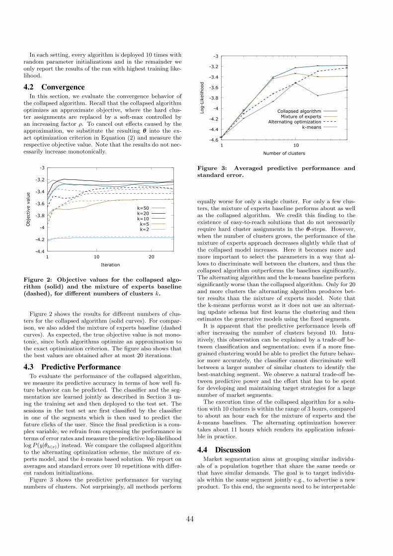
In each setting, every algorithm is deployed 10 times withrandom parameter initializations and in the remainder weonly report the results of the run with highest training like-lihood.
4.2 ConvergenceIn this section, we evaluate the convergence behavior of
the collapsed algorithm. Recall that the collapsed algorithmoptimizes an approximate objective, where the hard clus-ter assignments are replaced by a soft-max controlled byan increasing factor ρ. To cancel out effects caused by theapproximation, we substitute the resulting θ into the ex-act optimization criterion in Equation (2) and measure therespective objective value. Note that the results do not nec-essarily increase monotonically.
-4.4
-4.2
-4
-3.8
-3.6
-3.4
-3.2
-3
1 10 20
Obje
ctiv
e va
lue
Iteration
k=50k=20k=10k=5k=2
Figure 2: Objective values for the collapsed algo-rithm (solid) and the mixture of experts baseline(dashed), for different numbers of clusters k.
Figure 2 shows the results for different numbers of clus-ters for the collapsed algorithm (solid curves). For compar-ison, we also added the mixture of experts baseline (dashedcurves). As expected, the true objective value is not mono-tonic, since both algorithms optimize an approximation tothe exact optimization criterion. The figure also shows thatthe best values are obtained after at most 20 iterations.
4.3 Predictive PerformanceTo evaluate the performance of the collapsed algorithm,
we measure its predictive accuracy in terms of how well fu-ture behavior can be predicted. The classifier and the seg-mentation are learned jointly as described in Section 3 us-ing the training set and then deployed to the test set. Thesessions in the test set are first classified by the classifierin one of the segments which is then used to predict thefuture clicks of the user. Since the final prediction is a com-plex variable, we refrain from expressing the performance interms of error rates and measure the predictive log-likelihoodlogP (y|θh(x)) instead. We compare the collapsed algorithmto the alternating optimization scheme, the mixture of ex-perts model, and the k-means based solution. We report onaverages and standard errors over 10 repetitions with differ-ent random initializations.
Figure 3 shows the predictive performance for varyingnumbers of clusters. Not surprisingly, all methods perform
-4.6
-4.4
-4.2
-4
-3.8
-3.6
-3.4
-3.2
-3
1 10
Log-L
ikel
ihoo
d
Number of clusters
Collapsed algorithmMixture of experts
Alternating optimizationk-means
Figure 3: Averaged predictive performance andstandard error.
equally worse for only a single cluster. For only a few clus-ters, the mixture of experts baseline performs about as wellas the collapsed algorithm. We credit this finding to theexistence of easy-to-reach solutions that do not necessarilyrequire hard cluster assignments in the θ-steps. However,when the number of clusters grows, the performance of themixture of experts approach decreases slightly while that ofthe collapsed model increases. Here it becomes more andmore important to select the parameters in a way that al-lows to discriminate well between the clusters, and thus thecollapsed algorithm outperforms the baselines significantly.The alternating algorithm and the k-means baseline performsignificantly worse than the collapsed algorithm. Only for 20and more clusters the alternating algorithm produces bet-ter results than the mixture of experts model. Note thatthe k-means performs worst as it does not use an alternat-ing update schema but first learns the clustering and thenestimates the generative models using the fixed segments.
It is apparent that the predictive performance levels offafter increasing the number of clusters beyond 10. Intu-itively, this observation can be explained by a trade-off be-tween classification and segmentation: even if a more fine-grained clustering would be able to predict the future behav-ior more accurately, the classifier cannot discriminate wellbetween a larger number of similar clusters to identify thebest-matching segment. We observe a natural trade-off be-tween predictive power and the effort that has to be spentfor developing and maintaining target strategies for a largenumber of market segments.
The execution time of the collapsed algorithm for a solu-tion with 10 clusters is within the range of 3 hours, comparedto about an hour each for the mixture of experts and thek-means baselines. The alternating optimization howevertakes about 11 hours which renders its application infeasi-ble in practice.
4.4 DiscussionMarket segmentation aims at grouping similar individu-
als of a population together that share the same needs orthat have similar demands. The goal is to target individu-als within the same segment jointly e.g., to advertise a newproduct. To this end, the segments need to be interpretable
44

Mon Tue Wed Thu Fri Sat Sun
Rel
ativ
e vo
lum
e
Cluster 1
Mon Tue Wed Thu Fri Sat Sun
Rel
ativ
e vo
lum
e
Cluster 2
Mon Tue Wed Thu Fri Sat Sun
Rel
ativ
e vo
lum
e
Cluster 3
Mon Tue Wed Thu Fri Sat Sun
Rel
ativ
e vo
lum
e
Cluster 4
Figure 5: Click volumes of categories over time for the four clusters.
Cluster 1 Cluster 2
Cluster 3 Cluster 4
Figure 4: Visualization of click frequencies for thefive most frequent link locations using four clusters.
to derive a concise description of the segments that can beconverted into a segment-specific targeting strategy.
In our collapsed algorithm, generative models in each seg-ment encode the contained behavior and interest. The flex-ibility of the probabilistic inference machinery allows us toproject the behavior onto discriminative variables to visu-alize different characteristics of the clusters. In this sectionwe give two examples for such projections to visualize dif-ferently distributed user behavior across the clustering. Forsimplicity, we use a solution with four clusters.
The first example shows a visualization of segment-specificuser clicks in terms of their location on the Web page. In-cluding the location of clicks is necessary for altering the lay-out dynamically as changes in frequently clicked areas willhave impact the behavior more than substituting a redun-dant and less clicked widget. We focus on the five modulesof the Web site that receive the highest number of clicks inthe data.
Figure 4 shows the results. Segments 2, 3, and 4 exhibitvery similar click behavior in terms of the clicked modules.By contrast, cluster 1 differs significantly in the usage of theWeb components. On average, users in cluster 1 prefer thelocation visualized in black over the alternatives compared
to users in the other segments. This observation could be ex-ploited to directly devise target strategies. While membersof cluster 2–4 should be addressed by changing the contentof the modules visualized in gray or dark blue, users in thefirst segment could also be triggered by the module encodedin black.
Analogously, the behavior could be projected on the cat-egories to visualize the respective distribution of categoriesfor each segment. However, we choose to show a more inter-esting projection for lack of space. The incorporation of thetimestamps of the sessions allows us to visualize the clus-ters in time. As the feature representation of timestampsencompasses one week, Figure 5 shows the average categorydistribution across the days of the week where different col-ors correspond to different categories.3
Apparently, the clusters do not only differ in terms of thecategories but also specialize on certain periods in time be-cause the segments are optimized using all available data,that is, attribute and behavior encoding variables. The firstcluster clearly specializes on Sundays and is characterized bya clean topic distribution. The three other cluster also pos-sess dominant categories but focuses more on working daysthan on weekends. Cluster 4 contains the most diverse set ofcategories and acts like a basin for categories that are not aseasy to discriminate. Here it becomes obvious that a solu-tion with only four clusters may not be optimal for the taskat hand. When we increase the maximal number clusters,the category distribution of clusters becomes cleaner that isless categories are likely. Additionally, clusters adapt betterto specialized periods such as working days or weekends forlarger k.
Taking various such projections into account describessegments from different angles and helps to find a concisetargeting strategy. For instance, knowing the articles thatare likely to be read in an ongoing session helps to addressthe respective user in various ways including displaying ads.Incorporating context informations such as the click behav-ior of the segments, finally allows for tailoring web pages toeach segment and to increase the overall user experience.
5. CONCLUSIONWe studied discriminative clustering for structured and
complex response variables that can be represented as gen-erative models. The problem setting matches market seg-mentation tasks where populations are to be segmented intodisjoint groups. Solving market segmentation-like problemsappropriately not only involves a clustering of the individu-als but also learning a classifier that discriminates well be-
3Colors are again reused due to the large number of cate-gories.
45

tween the segments, for instance to allow for classifying newcustomers to one of the groups. The two components needto be learned jointly and have access to different pieces ofinformation about the individuals: the classifier needs togroup individuals on the basis of a priori available infor-mations while the clustering aims at grouping people withsimilar (future) needs or behavior.
We devised two algorithms based on alternating optimiza-tion and collapsed inference, respectively. Empirical resultsshowed that the collapsed variant is not only more efficientbut also predicts accurately the click behavior of users forYahoo! News. The generative nature of the clustering ledto interpretable clusters. We showed how projections of theclustering on only a few variables allowed for targeting thedetected segments individually and contributed to user un-derstanding.
Our approach is not restricted to Yahoo! News and cangenerally be applied to arbitrary market segmentation tasksand other Web sites to improve the overall user experience.As our approach is orthogonal to personalized approaches,future work will study the integration of both frameworks.
AcknowledgementsPart of this work was supported by the German ScienceFoundation under the reference number GA 1615/1-1.
References[1] N. Bansal, A. Blum, and S. Chawla. Correlation
clustering. Machine Learning, 56(1-3):89–113, 2004.
[2] S. Bickel and T. Scheffer. Multi-view clustering. InProceedings of the IEEE international conference ondata mining. Citeseer, 2004.
[3] U. Brefeld, P. Geibel, and F. Wysotzki. Supportvector machines with example dependent costs. InProceedings of the European Conference on MachineLearning, 2003.
[4] R. D’Andrade. U-statistic hierarchical clustering.Psychometrika, 4:58–67, 1978.
[5] F. De la Torre and T. Kanade. Discriminative clusteranalysis. In Proceedings of the 23rd internationalconference on Machine learning, pages 241–248. ACM,2006.
[6] A. Dempster, N. Laird, and D. Rubin. Maximumlikelihood from incomplete data via the em algorithm.Journal of the Royal Statistical Society. Series B(Methodological), pages 1–38, 1977.
[7] P. D’Urso and L. D. Giovanni. Temporalself-organizing maps for telecommunications marketsegmentation. Neurocomput., 71:2880–2892, 2008.
[8] R. Gomes, A. Krause, and P. Perona. Discriminativeclustering by regularized information maximization. InAdvances in Neural Information Processing Systems,2010.
[9] J. Huang, G. Tzeng, and C. Ong. Marketingsegmentation using support vector clustering. Expertsystems with applications, 32(2):313–317, 2007.
[10] R. Jacobs, M. Jordan, S. Nowlan, and G. Hinton.Adaptive mixtures of local experts. Neuralcomputation, 3(1):79–87, 1991.
[11] S. C. Johnson. Hierarchical clustering schemes.Psychometrika, 2:241–254, 1967.
[12] M. Jordan and R. Jacobs. Hierarchical mixtures ofexperts and the em algorithm. Neural computation,6(2):181–214, 1994.
[13] M. Y. Kiang, M. Y. Hu, and D. M. Fisher. Anextended self-organizing map network for marketsegmentation – a telecommunication example.Decision Support Systems, 42:36–47, 2006.
[14] S. P. Lloyd. Least square quantization in pcm. IEEETransactions on Information Theory, 28(2):129–137,1982.
[15] G. Mann, R. McDonald, M. Mohri, N. Silberman, andD. Walker. Efficient large-scale distributed training ofconditional maximum entropy models. Advances inNeural Information Processing Systems, 22:1231–1239,2009.
[16] M. Namvar, M. Gholamian, and S. KhakAbi. A twophase clustering method for intelligent customersegmentation. In 2010 International Conference onIntelligent Systems, Modelling and Simulation, pages215–219. IEEE, 2010.
[17] J. Sinkkonen, S. Kaski, and J. Nikkila. Discriminativeclustering: Optimal contingency tables by learningmetrics. Machine Learning: ECML 2002, pages109–137, 2002.
[18] K. Wagstaff, C. Cardie, S. Rogers, and S. Schrodl.Constrained k-means clustering with backgroundknowledge. In Proceedings of the InternationalConference on Machine Learning, 2001.
[19] M. Wedel and W. Kamakura. Market segmentation:conceptual and methodological foundations, volume 8.Springer, 2000.
[20] L. Xu, J. Neufeld, B. Larson, and D. Schuurmans.Maximum margin clustering. Advances in neuralinformation processing systems, 17:1537–1544, 2005.
[21] J. Ye, Z. Zhao, and M. Wu. Discriminative k-meansfor clustering. In Advances in Neural InformationProcessing Systems, 2007.
[22] W. Yu and G. Qiang. Customer segmentation of portbased on the multi-instance kernel k-aggregateclustering algorithm. In Management Science andEngineering, 2007. ICMSE 2007. InternationalConference on, pages 210–215, 2007.
[23] B. Zhao, J. Kwok, and C. Zhang. Maximum marginclustering with multivariate loss function. In DataMining, 2009. ICDM’09. Ninth IEEE InternationalConference on, pages 637–646. IEEE, 2009.
[24] B. Zhao, F. Wang, and C. Zhang. Efficient multiclassmaximum margin clustering. In Proceedings of the25th international conference on Machine learning,pages 1248–1255. ACM, 2008.
46

Chapter 6
Discussion
All presented papers advance the state of the art in prediction with mixture modelsin specific ways. The following chapter discusses how the thesis as a whole relatesto previous literature and how the contributions of the individual papers fit into theoverall picture. At first a discussion about existing general approaches to predictionwith mixture models is necessary.
Mixture of experts [Jordan 94] is a generic framework for learning predictive mix-ture models, used e.g. successfully for EEG signal classification [Subasi 07], pedes-trian classification [Enzweiler 11], and protein structure prediction [MacDonald 12].It makes use of the fact that the models in each mixture component are efficientlytractable, while the learned model overall is complex. The mixture components areoptimized with respect to the predictive accuracy of the overall model. However,this generic approach can not take into account domain-specific knowledge about theactual cluster structure in the data without additional feature engineering.
Deep neural networks [Hinton 06], which have recently been successfully appliedto various applications, e.g. [Mohamed 11], [Mohamed 12], [Socher 12], and [Yu 12],can also be interpreted as mixture models. They consist of multiple layers, each witha predetermined number of binary feature detectors. The bottom-most layer encodesthe input data. Within each layer, the feature detectors are trained to maximize theprobablity of the states of the lower layers. Finally, the top-most layer has additionalweights that are optimized to predict a target variable. Each feature detector in thetop layer is a predictor for the target variable. Viewing the approach in terms ofmixture models provides an insight into why deep belief networks work so well. Onecan regard each subset of feature detectors within a layer of the network as a mixturecomponent c. Predictions for the activations in the layer above y given the layerbelow x are computed with the usual P (y|x) =
∑c P (c|x)P (y|c), using sampling
or mean-field approximation [Lee 09] to approximate the sum over c. Now findinggood parameters for both P (c|x) and P (y|c) is a challenge, because in general theoptimization problem is highly non-convex, and optimization procedures can easilyget stuck in poor local optima. But because the subsets of feature detectors in deepbelief networks share parameters with each other, in effect one can utilize a numberof components that is exponential in the number of detectors. Thus even if mostcomponents have little predictive power due to poor local optima, there is a highchance that at least some of the components are useful. Furthermore, P (c|x) isdefined in terms of the joint probability distribution P (x, c), which can be optimizedusing unlabeled data, which is usually available in much greater abundance than
47

labeled data. Thus, unsupervised pre-training can be leveraged to obtain a goodinitialization for the component parameters. The recently studied improvement ofdeep neural networks called dropout provides an indication for the correctness of thishypothetical explanation [Hinton 12]. Here, for each stochastic gradient update step,each detector is removed with probability 0.5. This makes training different subsetsof detectors more explicit, and consequently improves accuracy. Thus far deep neuralnetworks have been used for applications like visual object recognition and speechrecognition. Adapting them to other types of data like text is still an open challenge.Though they have been used for textual data with some success [Socher 11], theproblem of capturing the complex sequential dependencies of natural language is stillnot generally solved.
A conceptually similar, but methodically different approach are support vectormachines for structured outputs with latent variables [Yu 09]. Here, a set of hiddenvariables is introduced, where each possible realization c can be seen as a mixturecomponent. For prediction, the decision function is maximized over the components,instead of averaged. Compared to deep belief networks, the relationship betweeninput and hidden variables can not be pre-trained using unlabeled data, because it isa purely discriminative approach and there is no notion of a distribution over inputs.This does, however, make it easier to utilize all sorts of data types.
A large class of generative mixture models can be subsumed under the termtopic models, overviewed in [Steyvers 07] and [Teh 10]. Often-used frameworks arehierarchical dirichlet processes [Teh 06] and Indian Buffet processes [Griffiths 06].Mostly used for textual data, mixture components are topics c, which are defined asdistributions over words in the vocabulary. Words y in a document x are predictedin the usual fashion as P (y|x) =
∑c P (c|x)P (y|x). For example in the application of
document retrieval, the match of a document x to a query word y can be computedvia P (y|x) [Wei 06]. In order for topic models to work as intended, the distributionsover topics given a document P (c|x) are often enforced to be sparse via a Dirichletprior [Blei 03]. Each document is thus associated with only a small number of topics,while not being as restrivtive as requiring a single topic for each document.
In most cases, learning mixture models involves either solving a non-convex opti-mization problem, for which the globally optimal solution can not be found efficiently,or in the fully Bayesian setting, computing an intractable integral. There are sev-eral general approaches to address this problem. One of them is the EM algorithm[Dempster 77], which alternates between maximizing a lower bound of the completedata likelihood and constructing a new lower bound at the current solution. It isguaranteed to find at least a local optimum of the optimization problem. Anotherclass of approaches are variational methods [Attias 99], which approximate the jointdata distribution with a combination of simpler distributions for which the solutioncan be found efficiently. Furthermore there have been developed Markov chain MonteCarlo algorithms such as the Gibbs sampler [Smith 93] which in the limit of infinitelymany sampling iterations generates samples from the true posterior distribution overthe model parameters. The methods in this thesis use several variants of those ap-proaches, as well as a simple greedy procedure when it is appropriate such as inSection 2.5.
48

6.1 Application-oriented Modelling
In order to use the available training data as effectively as possible, the used modelhas to be tailored to each application specifically. The papers of this thesis followthis principle for four different applications and thereby provide new methods to dealwith them more effectively.
In Chapter 2 [Haider 09], the framework of Bayesian model-based clustering isextended to handle vectors of binary features that are not independent. For textualdata, the independence assumption is clearly unjustified. Hence the demonstratedincrease in predictive accuracy through allowing dependencies in the input space wasexpected. Tractability of the model is maintained by using a novel pretrained featuretransformation, which is specifically optimized in order to minimize the approxima-tion error induced by the independence assumption in the transformed space. Thusthe paper broadens the spectrum of classes of observations for which a proper mixturemodel can be formulated and efficiently inferred.
For observations that can be abstracted into a graph where the presence of edgesconstitutes evidence for shared cluster membership and the absence of edges con-situtes only weak evidence against, Chapter 3 [Haider 12b] provides a novel way ofmodeling the posterior distribution over clusterings. It depends only on the cliques ofthe graph, and does not have to make any assumptions about the process generatingthe observations. Compared to previous approaches for graph partitioning [Ng 02],it does not provide only a point estimate, but a complete distribution. Furthermore,the number of clusters does not have to be specified in advance.
In Chapter 4 [Dick 08] the main advance is that the developed method not onlyestimates a single set of imputations for the missing values, but instead a distributionover imputation sets. This is more appropriate because it reflects the remaininguncertainty about the imputed values. This is similar to replacing a maximum-a-posteriori point estimate with full Bayesian inference.
The optimization problem stated in Chapter 5 [Haider 12a] is the first formulationof the market segmentation problem that neither needs to define the classificationcriteria or the cluster parameters beforehand nor neglects the fact that each trainingexample has to be predicted by a single cluster. By combining the goals of separabilityand homogeneity into a single objective function, there is no intermediate step thatrelies on heuristics involved.
6.2 Improvement of Predictive Power
In full Bayesian approaches of mixture models, there is no set of parameters thatgets optimized. Thus there is only one way of pursuing that the resulting mixturemodel (respectively distribution over mixture models) is useful for prediction: theconstructor of the model has to ensure that it matches the real generative processor the dependencies between observables and latent variables as closely as possible.However if the models include hyperparameters, those can be optimized with respectto the predictive accuracy. In Chapter 2 [Haider 09] this is accomplished throughthe use of the precision parameter σ that governs the probability of deviations offeature frequencies compared to the training set. Indirectly this parameter controlsthe granularity of the resulting clusterings, which greatly influences predictions. By
49

tuning it on a hold-out dataset, see Section 2.6, we can maximize predictive accuracy.
The concentration hyperparameters αa and αs in Chapter 3 [Haider 12b] playa similar role. They control how likely it is that a new email originated from adifferent botnet than all previous emails from the same IP address or spam campaign,respectively. They, too, can be tuned on a hold-out set as in Section 3.4 to optimizepredictive power of a model that by itself does not include an optimization criterionthat takes prediction accuracy into account.
Approaches based on expected risk minimization provide the possibility to definethe risk and the resulting objective funtion in terms of the prediction accuracy. In Sec-tion 4.3 [Dick 08] the risk is defined as a function of a decision function which dependson the estimated mixture, such that the mixture itself is optimized with regard toaccuracy. The same is true for the optimization problem in Chapter 5 [Haider 12a].There the relationship between the clustering and the resulting prediction is moredirect than in previous work.
All four presented papers include evidence that in their respective applicationsthe use of mixture models leads to an improvement compared to the correspondingsingle-component models. Single-component baselines are either explicitly mentionedor covered as special cases of one of the reference methods:
In the spam campaign detection application of Chapter 2 [Haider 09], the hyper-parameter σ controls the granularity of the clustering. In the limit of σ → ∞ thesolution degrades to a single cluster, and thus to prediction with a single-componentmodel. Since σ is tuned with respect to predictive accuracy, this case is implicitlyincluded in the evaluation and shown to perform worse than the mixture model. An-other single-component baseline is the one-class support vector machine, which isexplicitly shown to perform worse, see Section 2.6.
The case with the application of botnet detection in Chapter 3 [Haider 12b] issimilar. Here the hyperparameters also enforce in the limit of αa → 0 and αs → 0a single-cluster solution. As with σ above, they are tuned with respect to predictiveaccuracy, such that the single-component model is implicitly part of the evaluation.
In the application of classifying emails with missing values in Chapter 4 [Dick 08],we compare the method of finding a mixture of imputations for the missing values toseveral methods for finding a single set of imputations. In each case, the single set ofimputations is used as a prior for the distribution over imputations. The evaluationin Section 4.6 shows that for almost all combinations of single imputation methodsand datasets learning a distribution over imputations increases predictive accuracysignificantly.
In Chapter 5 [Haider 12a] about market segmentation, we evaluate the methodfor different numbers of clusters, including one. The results in Section 5.4 show thatpredictive accuracy rises steeply with increasing number of clusters in the beginning,and then levels off.
6.3 Evaluability
The third aspect of the overall research question of this thesis is how prediction withmixture models can serve as a means to evaluating the cluster structure underlying themixture. One of the approaches that can be taken in order to evaluate the accuracy ofclusterings found by a method is to use synthetic data [Thalamuthu 06]. One simply
50

generates artificial data that is assumed to have the same characteristics as the realdata, and compares the found clustering to the clusters in the generated data. Butthis approach suffers from the flaw that one has to make strong assumptions aboutthe characteristics of the real data. If those assumptions are wrong, the obtainedevaluation is also incorrect.
Generative models such as topic models can be evaluated by computing the jointlikelihood of the training set, see e.g. [Heller 05]. In the same fashion one can selectdifferent models or optimize their hyperparameters. This is reasonable for choosingfew parameters of a single generative model family, but it can not be reliably usedfor choosing the family of the model: It is always possible to construct a model witha prior that assigns maximum probability mass to all training examples and zeroprobability to all others. Thus it compares favorably to all other models under thecriterion of training set likelihood, but is actually useless. Consider for example amixture model that assigns each example to its own cluster, with parameters thatassign probability one to the example in the cluster, and a prior over cluster param-eters that is only supported on the values taken by those clusters. Here, the sumof marginal likelihoods over training examples is one. Consequentially, the marginallikelihood of an example not included in the training set is zero. It is more accu-rate to evaluate a mixture model by computing (approximately) the probability ofheld-out documents [Wallach 09]. This is a special case of assessing the accuracy of aclustering by measuring its predictive power. However this works only for generativemodels, and thus can not be used to compare, e.g., a generative model to a heuristicclustering algorithm.
In Chapter 2 [Haider 09], the found clustering of emails into campaigns could inprinciple be evaluated by itself, although that would involve costly manual labeling ofthe test data. Using the usefulness of the clustering as an intermediate step of spamfiltering is much cheaper, since emails labeled as spam or non-spam are readily avail-able. And this is better than using some intrinsic measure of clustering quality, likeBayesian information criterion [Schwarz 78]. Intrinsic measures are not application-specific, and there is no guarantee that a particular criterion works well in a certaindomain.
The application of finding botnets in Chapter 3 [Haider 12b] does not lend itselfto a supervised evaluation of the found clusterings by itself. Emails arrive fromarbitrary hosts that are not under the experimenter’s control, and thus he or shecannot obtain the information to which botnet each host actually belongs. In Section3.4 we evaluate the clusterings using only observable information, by measuring theaccuracy of predicting the campaign of an email given its IP address, utilizing thedistributions over campaigns and botnets arising from the inferred clustering. Thismethod of evaluation is the only alternative to intrinsic evaluation criteria, whichhave the aforementioned drawbacks. Prior published work does not evaluate thefound clusterings at all, and instead is restricted to qualitative analysis.
For the application of learning a classifier from data with missing values studied inChapter 4 [Dick 08], there exists the theoretical possibility of evaluating the processthat generates the distribution over imputations, but not the imputations per se.If one would take a subset of the training examples with complete data, eradicatesome of the observations, and then apply any method that deals with missing valuesby imputing one or more values, then one could compare the found imputationswith the original, erased values. We have not done so in our experiments because,
51

in the application, only the resulting predictive accuracy is of importance. In thiscase, measuring predictive accuracy not only allows us to indirectly evaluate thedistribution over imputations for training examples which are actually incompletelyobserved, but the evaluation criterion is even more relevant to the application thana direct evaluation of the imputations.
A different case presents itself with the abstract problem setting of market segmen-tation in Chapter 5 [Haider 12a]. There exist many suggestions of a priori criteriato segment markets. But these are mostly concerned about homogeneity and notseparability. Even homogeneity is only directly pursued with respect to for exampledemographic attributes, when in fact homogeneity is desired with respect to futurebehavior that is relevant to the vendor-client relationship. In Section 5.3 the seg-ments are optimized with respect to exactly the observed behavior of the trainingexamples. Also, separability is taken into account in the only natural way. Insteadof trading off separability and homogeneity in an ad hoc way, the predictive powerof the model when actually applied to separating the training examples is optimized.Thus the optimization criterion itself takes into account the usefulness of the foundpartitioning.
52

Bibliography
[Attias 99] Hagai Attias. Inferring parameters and structure of latent vari-able models by variational Bayes. In Proceedings of the FifteenthConference on Uncertainty in Artificial Intelligence, pages 21–30.Morgan Kaufmann Publishers Inc., 1999.
[Blei 03] David M Blei, Andrew Y Ng & Michael I Jordan. Latent dirichletallocation. Journal of Machine Learning Research, vol. 3, pages993–1022, 2003.
[Dempster 77] Arthur P Dempster, Nan M Laird & Donald B Rubin. Maximumlikelihood from incomplete data via the EM algorithm. Journal ofthe Royal Statistical Society. Series B (Methodological), pages 1–38, 1977.
[Dick 08] Uwe Dick, Peter Haider & Tobias Scheffer. Learning from incom-plete data with infinite imputations. In Proceedings of the 25th In-ternational Conference on Machine Learning, pages 232–239. ACM,2008.
[Enzweiler 11] Markus Enzweiler & Dariu M Gavrila. A multilevel mixture-of-experts framework for pedestrian classification. IEEE Transactionson Image Processing, vol. 20, no. 10, pages 2967–2979, 2011.
[Geweke 11] John Geweke & Gianni Amisano. Hierarchical Markov normal mix-ture models with applications to financial asset returns. Journal ofApplied Econometrics, vol. 26, no. 1, pages 1–29, 2011.
[Griffiths 06] Tom Griffiths & Zoubin Ghahramani. Infinite latent feature modelsand the Indian buffet process. In Advances in Neural InformationProcessing Systems 18, pages 475–482. MIT Press, Cambridge, MA,2006.
[Haider 09] Peter Haider & Tobias Scheffer. Bayesian clustering for email cam-paign detection. In Proceedings of the 26th Annual InternationalConference on Machine Learning, pages 385–392. ACM, 2009.
[Haider 12a] Peter Haider, Luca Chiarandini & Ulf Brefeld. Discriminative clus-tering for market segmentation. In Proceedings of the 18th ACMSIGKDD International Conference on Knowledge Discovery andData Mining, pages 417–425. ACM, 2012.
53

[Haider 12b] Peter Haider & Tobias Scheffer. Finding Botnets Using MinimalGraph Clusterings. In Proceedings of the 29th International Con-ference on Machine Learning, pages 847–854, 2012.
[Heller 05] Katherine A Heller & Zoubin Ghahramani. Bayesian hierarchicalclustering. In Proceedings of the 22nd International Conference onMachine Learning, pages 297–304. ACM, 2005.
[Hinton 06] Geoffrey E Hinton & Ruslan R Salakhutdinov. Reducing the dimen-sionality of data with neural networks. Science, vol. 313, no. 5786,pages 504–507, 2006.
[Hinton 12] Geoffrey E. Hinton, Nitish Srivastava, Alex Krizhevsky, IlyaSutskever & Ruslan Salakhutdinov. Improving neural net-works by preventing co-adaptation of feature detectors. CoRR,vol. abs/1207.0580, 2012.
[Jordan 94] Michael I Jordan & Robert A Jacobs. Hierarchical mixtures ofexperts and the EM algorithm. Neural Computation, vol. 6, no. 2,pages 181–214, 1994.
[Lee 09] Honglak Lee, Roger Grosse, Rajesh Ranganath & Andrew Y Ng.Convolutional deep belief networks for scalable unsupervised learn-ing of hierarchical representations. In Proceedings of the 26th An-nual International Conference on Machine Learning, pages 609–616.ACM, 2009.
[MacDonald 12] Ian M MacDonald. Protein structural domain boundary prediction:A mixture of experts approach. AV Akademikerverlag, 2012.
[McNicholas 10] Paul D McNicholas & Thomas Brendan Murphy. Model-based clus-tering of microarray expression data via latent Gaussian mixturemodels. Bioinformatics, vol. 26, no. 21, pages 2705–2712, 2010.
[Mohamed 11] A-R Mohamed, Tara N Sainath, George Dahl, Bhuvana Ramabhad-ran, Geoffrey E Hinton & Michael A Picheny. Deep belief networksusing discriminative features for phone recognition. In IEEE Inter-national Conference on Acoustics, Speech and Signal Processing,pages 5060–5063. IEEE, 2011.
[Mohamed 12] Abdel-rahman Mohamed, George E Dahl & Geoffrey Hinton.Acoustic modeling using deep belief networks. IEEE Transactionson Audio, Speech, and Language Processing, vol. 20, no. 1, pages14–22, 2012.
[Ng 02] Andrew Y Ng, Michael I Jordan, Yair Weisset al. On spectral clus-tering: Analysis and an algorithm. Advances in Neural InformationProcessing Systems, vol. 2, pages 849–856, 2002.
[Povey 10] Daniel Povey, Lukas Burget, Mohit Agarwal, Pinar Akyazi, KaiFeng, Arnab Ghoshal, Ondrej Glembek, Nagendra Kumar Goel,Martin Karafiat, Ariya Rastrowet al. Subspace Gaussian mixture
54

models for speech recognition. In IEEE International Conference onAcoustics Speech and Signal Processing, pages 4330–4333. IEEE,2010.
[Schwarz 78] Gideon Schwarz. Estimating the dimension of a model. The Annalsof Statistics, vol. 6, no. 2, pages 461–464, 1978.
[Smith 93] Adrian FM Smith & Gareth O Roberts. Bayesian computation viathe Gibbs sampler and related Markov chain Monte Carlo methods.Journal of the Royal Statistical Society. Series B (Methodological),pages 3–23, 1993.
[Socher 11] Richard Socher, Cliff C. Lin, Andrew Y. Ng & Christopher D. Man-ning. Parsing Natural Scenes and Natural Language with RecursiveNeural Networks. In Proceedings of the 26th International Confer-ence on Machine Learning (ICML), 2011.
[Socher 12] Richard Socher, Brody Huval, Bharath Bath, Christopher D Man-ning & Andrew Ng. Convolutional-recursive deep learning for 3Dobject classification. In Advances in Neural Information ProcessingSystems, pages 665–673, 2012.
[Steyvers 07] Mark Steyvers & Tom Griffiths. Probabilistic topic models. Hand-book of latent semantic analysis, vol. 427, no. 7, pages 424–440,2007.
[Subasi 07] Abdulhamit Subasi. EEG signal classification using wavelet featureextraction and a mixture of expert model. Expert Systems withApplications, vol. 32, no. 4, pages 1084–1093, 2007.
[Teh 06] Yee Whye Teh, Michael I Jordan, Matthew J Beal & David M Blei.Hierarchical dirichlet processes. Journal of the American StatisticalAssociation, vol. 101, no. 476, 2006.
[Teh 10] Yee Whye Teh & Michael I Jordan. Hierarchical Bayesian nonpara-metric models with applications. Bayesian Nonparametrics: Princi-ples and Practice, pages 158–207, 2010.
[Thalamuthu 06] Anbupalam Thalamuthu, Indranil Mukhopadhyay, Xiaojing Zheng& George C Tseng. Evaluation and comparison of gene clusteringmethods in microarray analysis. Bioinformatics, vol. 22, no. 19,pages 2405–2412, 2006.
[Wallach 09] Hanna M Wallach, Iain Murray, Ruslan Salakhutdinov & DavidMimno. Evaluation methods for topic models. In Proceedings ofthe 26th Annual International Conference on Machine Learning,pages 1105–1112. ACM, 2009.
[Wei 06] Xing Wei & W Bruce Croft. LDA-based document models for ad-hocretrieval. In Proceedings of the 29th Annual International ACMSIGIR Conference on Research and Development in InformationRetrieval, pages 178–185. ACM, 2006.
55

[Yu 09] Chun-Nam John Yu & Thorsten Joachims. Learning structuralSVMs with latent variables. In Proceedings of the 26th AnnualInternational Conference on Machine Learning, pages 1169–1176.ACM, 2009.
[Yu 12] Dong Yu, Frank Seide & Gang Li. Conversational Speech Tran-scription Using Context-Dependent Deep Neural Networks. In Pro-ceedings of the 29th International Conference on Machine Learning,2012.
[Zhang 11] Cha Zhang, Michael Cohen, Yong Rui & Ting Yu. Image segmenta-tion using spatial-color Gaussian mixture models, February 8 2011.US Patent 7,885,463.
56