PREDICTION OF YARN TENACITY OF RAW COTTON USING …
115
PREDICTION OF YARN TENACITY OF RAW COTTON USING FUZZY INFERENCE SYSTEM by Shaukat Ahmed Department of Industrial and Production Engineering Bangladesh University of Engineering and Technology Dhaka, Bangladesh.
Transcript of PREDICTION OF YARN TENACITY OF RAW COTTON USING …

PREDICTION OF YARN TENACITY OF RAW COTTON USING FUZZY INFERENCE SYSTEM
by
Shaukat Ahmed
Department of Industrial and Production Engineering Bangladesh University of Engineering and Technology
Dhaka, Bangladesh.
PREDICTION OF YARN TENACITY OF RAW COTTON USING
FUZZY INFERENCE SYSTEM
by
Shaukat Ahmed
A project submitted to the Department of Industrial and Production Engineering, Bangladesh University of Engineering and Technology (BUET), Dhaka, in partial fulfillment of the requirements for the degree of Master of Engineering (M.Engg.) in Advanced Engineering Management.
Department of Industrial and Production Engineering Bangladesh University of Engineering and Technology
Dhaka, Bangladesh. January 2014.
CERTIFICATE OF APPROVAL
The Project titled “PREDICTION OF YARN TENACITY OF RAW COTTON USING FUZZY INFERENCE SYSTEM” submitted by Shaukat Ahmed, Student No: 0411082125, Session: April/2011, has been accepted as satisfactory in partial fulfillment of the requirement for the degree of MASTER OF ENGINEERING IN ADVANCED ENGINEERING MANAGEMENT on January 25, 2014.
BOARD OF EXAMINERS
___________________________ Dr. Ferdous Sarwar Assistant Professor Chairman
Department of Industrial and Production Engineering, (Supervisor) Bangladesh University of Engineering and Technology (BUET) Dhaka – 1000,Bangladesh.
___________________________ Dr. Abdullahil Azeem Professor Member Department of Industrial and Production Engineering
Bangladesh University of Engineering and Technology (BUET) Dhaka – 1000,Bangladesh. ___________________________ Dr. Sultana Parveen Professor Member Department of Industrial and Production Engineering
Bangladesh University of Engineering and Technology (BUET) Dhaka – 1000, Bangladesh.

DECLARATION It is hereby declared that this thesis or any part of it has not been submitted elsewhere for the award of any degree or diploma.
Shaukat Ahmed

Dedication
To my parents.


i
ACKNOWLEDGEMENT
First of all, I would like to thank Allah for giving me the ability to complete this project.
Completing my Master degree is probably the most challenging activity of my life. The best
and worst moments of the journey have been shared with many people. It has been a great
privilege to spend several years in the Department of Industrial and Production Engineering
at Bangladesh University of Engineering & Technology and its members will always remain
dear to me.
My next debt of gratitude must go to my advisor Dr. Ferdous Sarwar. He patiently provided
the vision, encouragement and advice necessary for me to proceed through the program and
complete my dissertation. I want to thank him for his unflagging encouragement and serving
as a role model to me as a junior member of academia. He has been a strong and supportive
adviser to me throughout my graduate school career, but he has always given me great
freedom to pursue independent work.
Special thanks to my committee, Dr. Abdullahil Azeem and Dr. Sultana Parveen for their
support, guidance and helpful suggestions. Their guidance has served me well and I owe
them my heartfelt appreciation.
Members of NR Group, Otto Spinning Mills also deserve my sincerest thanks, their
friendship and assistance has meant more to me than I could ever express. I could not
complete my work without invaluable friendly assistance of them.
I wish to thank my parents. Their love provided my inspiration and was my driving force. I
owe them everything and wish I could show them just how much I love and appreciate them.
Also give thanks to my wife, whose love and encouragement allowed me to finish this
journey. My only son who has my heart, I will just give him a heartfelt “thanks.” I also want
to thank to my office mates for their unconditional support. Finally, I would like to dedicate
this work to my parents. I hope that this work makes them proud.

ii
ABSTRACT
Due to the wide variability of cotton fibre properties, such as fibre strength , Upper High
Mean Length (UHML), Uniformity Index(UI), Micronaire, Short Fibre % (SF%), Fibre
Elongation, Yellownes, Mean length, Neps, Maturity Ratio(MR) from bale to bale , the
aspect of cotton performance prediction is always very much tricky and arduous job. A large
number of predictive models have been exercised to prognosticate the yarn strength. By and
large, there are three distinguished modeling methods for predicting the yarn properties like
Mathematical models, Statistical regression models and Intelligent models.
A theoretical or Mathematical approach and an empirical or statistical approach both types of
models have their advantages and disadvantages. For instance, the mathematical models are
derived from the first principle analysis and have their basis in applied physics. Therefore,
they are appealing and capable of providing a better understanding of the complex
relationships between the yarn properties and the influencing parameters. However, firstly
these models always require simplified assumptions to make the mathematic tractable, and
the validity of the model depends on the validity of the assumptions. Secondly, the
mathematical models are associated with large prediction errors and therefore not reliable
enough to work in practical situations due to the uncertainties connected with the real world
dynamics. On the other hand, the empirical or statistical models are easy to develop but they
require the specialized knowledge of both statistical methods and designs of experiments.
Extensive experimentation and test and data gathering connected with measurement errors
can generate the `noise' in data. Unfortunately, these models are sensitive to the `noise'. Also
the present techniques are insufficient for precise modeling and predicting the complex non-
linear processes. The prediction accuracy of ANN has been acclaimed by most of the
researchers. However, ANN modeling has also received criticisms for acting like a ‘black
box’ without revealing much about the mechanics of the process. Some limitation of the
ANN modeling could be overcome by using fuzzy logic, which can effectively translate the
experience of a spinner into a set of expert system rules. It is quite possible to devise a fuzzy
logic based expert system which can predict yarn strength from the given input parameters.
iii
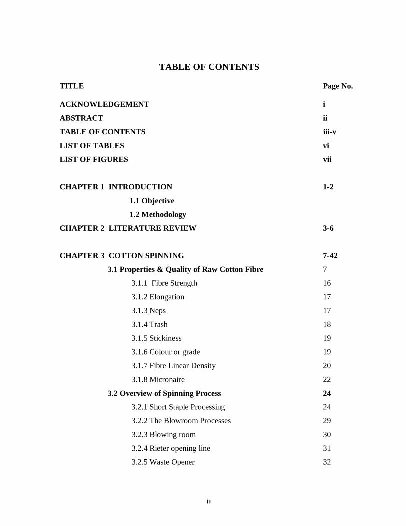
TABLE OF CONTENTS
TITLE Page No. ACKNOWLEDGEMENT i
ABSTRACT ii
TABLE OF CONTENTS iii-v
LIST OF TABLES vi
LIST OF FIGURES vii
CHAPTER 1 INTRODUCTION 1-2
1.1 Objective
1.2 Methodology
CHAPTER 2 LITERATURE REVIEW 3-6
CHAPTER 3 COTTON SPINNING 7-42
3.1 Properties & Quality of Raw Cotton Fibre 7
3.1.1 Fibre Strength 16
3.1.2 Elongation 17
3.1.3 Neps 17
3.1.4 Trash 18
3.1.5 Stickiness 19
3.1.6 Colour or grade 19
3.1.7 Fibre Linear Density 20
3.1.8 Micronaire 22
3.2 Overview of Spinning Process 24
3.2.1 Short Staple Processing 24
3.2.2 The Blowroom Processes 29
3.2.3 Blowing room 30
3.2.4 Rieter opening line 31
3.2.5 Waste Opener 32

iv
3.2.6 Blending/mixing 33
3.2.7 Optimum setting of cleaning 33
3.2.8 Basic actions in carding 33
3.2.9 Drawing 35
3.2.10 Autolevelling in Drawing 36
3.2.11 Roving & Ring spinning 39-42
CHAPTER 4 FUZZY LOGIC 43-55
4.1 Introduction 43
4.2 Difference of Fuzzy logic from conventional
control methods. 43
4.3 Use of Fuzzy logic 44
4.4 Logical operations 45
4.5 Fuzzy Subset 46
4.5.1 Logic Operations 47
4.6 Defuzzification 47
4.6.1 Selection Of Defuzzification Method 48
4.6.1.1 Centroid Method 48
4.6.1.2 Centre Of Sums Method 48
4.6.1.3 Mean Of Maxima (Mom) Defuzzification 49
4.7. Fuzzy Expert System 49
4.8 The Inference Process 50
4.9 Fuzzification 51
4.9.1 Inference 51
4.9.2 Composition 51
4.10 Membership Function 52
4.11 If-Then Rules 54
v
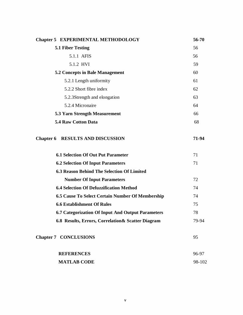
Chapter 5 EXPERIMENTAL METHODOLOGY 56-70
5.1 Fiber Testing 56
5.1.1 AFIS 56
5.1.2 HVI 59
5.2 Concepts in Bale Management 60
5.2.1 Length uniformity 61
5.2.2 Short fibre index 62
5.2.3Strength and elongation 63
5.2.4 Micronaire 64
5.3 Yarn Strength Measurement 66
5.4 Raw Cotton Data 68
Chapter 6 RESULTS AND DISCUSSION 71-94
6.1 Selection Of Out Put Parameter 71
6.2 Selection Of Input Parameters 71
6.3 Reason Behind The Selection Of Limited
Number Of Input Parameters 72
6.4 Selection Of Defuzzification Method 74
6.5 Cause To Select Certain Number Of Membership 74
6.6 Establishment Of Rules 75
6.7 Categorization Of Input And Output Parameters 78
6.8 Results, Errors, Correlation& Scatter Diagram 79-94
Chapter 7 CONCLUSIONS 95
REFERENCES 96-97
MATLAB CODE 98-102
vi
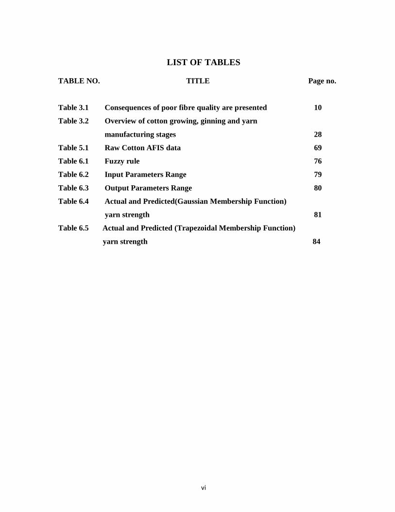
LIST OF TABLES
TABLE NO. TITLE Page no.
Table 3.1 Consequences of poor fibre quality are presented 10
Table 3.2 Overview of cotton growing, ginning and yarn
manufacturing stages 28
Table 5.1 Raw Cotton AFIS data 69
Table 6.1 Fuzzy rule 76
Table 6.2 Input Parameters Range 79
Table 6.3 Output Parameters Range 80
Table 6.4 Actual and Predicted(Gaussian Membership Function)
yarn strength 81
Table 6.5 Actual and Predicted (Trapezoidal Membership Function)
yarn strength 84

vii
LIST OF FIGURES
FIGURE NO. TITLE Page no. Figure 3.1 Various Textile Industry 9
Figure 3.2 Comb-sorter fibre array for a roller ginned
extra long staple fibre sample 16
Figure 3.3 Typical Fibrogram showing length measurement locations
on the fibre length diagram produced by the Fibro graph. 17
Figure 3.4 Photo of a fibre array comb for the HVI Fibrograph (length)
and strength tester. (CSIRO). 19
Figure 3.5 A nep is an entanglement of fibres resulting from
mechanical processing 19
Figure 3.6 The cross section of a cotton yarn showing the packing and
interaction of individual fibres. 21
Figure 3.7 Schematic simple representations of the arrangement of
fibres within a yarn. 22
Figure 3.8 Cross section of fibres that have similar Micronaire values
(samesurface area to weight ratios). 24
Figure 3.9 Fibre to yarn processing for cotton 26
Figure 3.10 Flow chart Cotton Ring Spinning 31
Figure 3.11 Rieter VarioSet Blowing room/Carding room 32
Figure 3.12 Trutschler Modular Opening Component Line 32
Figure 3.13 Carding and stripping actions 35
Figure3.14 Adrawframe with 8 doublings and an autolevelling unit 36
Figure 3.15 Fibre straightening during drafting 39
Figure 3.16 Diagram of a roving frame 41
Figure 5.1 Raw Cotton Sample 58
Figure 5.2 AFIS working Principle 59
Figure 6.1 Matlab Screen Shots of Fuzzy Expert System 73
Figure 6.2 Actual vs Predicted Yarn strength 87
Figure 6.3 Matrix Plot of Fibre Properties vs Yarn strength 89
1
CHAPTER 1
INTRODUCTION
The commercial value of a cotton fibre depends on its performance during spinning operation
and the properties of yarn (Yarn Strength, Elongation, Unevenness) that could be spun from
that fibre. A spinner is always very keen to know the achievable level of yarn properties
(Tenacity) because if he has a mindset about that cotton, then he can even churn his
experience to adjust the process parameters. However, due to the wide variability of cotton
fibre properties, such as fibre strength , Upper High Mean Length (UHML), Uniformity
Index(UI), Micronaire, Short Fibre % (SF%), Fibre Elongation, Yellowness, Mean length,
Neps, Maturity Ratio(MR) from bale to bale , the aspect of cotton performance prediction is
always very much tricky and arduous job. A large number of predictive models have been
exercised to prognosticate the yarn strength. The prediction of yarn strength acquires a
mammoth share among these models. By and large, there are essentially three distinguished
modeling tools for predicting the yarn properties, such as mathematical models, statistical
regression models and intelligent models like artificial neural network, fuzzy logic and case
based reasoning. Generally, the yarn properties are ascertained by processing a small quantity
of cotton to a particular count and then measuring the properties of yarn so produced. But it
is a time consuming and labor intensive process.
Mathematical models are very appealing as they are based on the theories of basic sciences
and give good understanding about the mechanics of the process. However, the prediction
accuracy of mathematical models is not very encouraging due to the assumptions used while
building the model. Statistical regression models are very easy to develop and beta
coefficient analysis give an indication about the relative importance of various inputs.
To counteract this problem, textile researchers have proposed various models relating fibre
and yarn properties. Fuzzy logic technique is the most commonly used method to predict the
yarn strength. The reason of its popularity steamed from the simplicity of this model.
The importance of Yarn Strength is huge for all type of Textile Products. Yarn strength
depends upon various parameters of fibres. However there is no such equations available

2
with which it is possible to predict the Yarn strength from the input parameters. With the
help of Fuzzy logic we can easily predict the Yarn strength.
1.1 Objectives with specific aims and possible outcomes The objectives of the proposed thesis work are:
To explore the new intelligent technologies and attempt to use them as new
approaches to predict and control yarn quality.
To develop a fuzzy expert system for the modeling of yarn tenacity using
fiber tenacity, mean length, micronaire and short fiber content as input
variables.
To maximize the production by minimizing the sampling time.
To compare the results of Fuzzy expert system with the actual yarn strength.
1.2 Outline of methodology The methodology would be as follows:
Data will be collected from different raw cotton bales by testing four
significant fibre properties (Mean Length, Short Fibre Content, Fibre
strength, Micronaire value) from two running cotton spinning mills of
Bangladesh.
Carded ring spun yarn of 30s (single count) would be produce and actual Yarn
tenacity or strength would be measure by Uster yarn Tester machine. A total
of 79 sample data of fibre properties and yarn strength would be taken.
A Fuzzy rule based inference system will be developed to predict yarn
tenacity to apply in the Cotton Spinning Mills of Bangladesh.
Comparison will be done between actual yarn strength value and the predicted
yarn strength obtained from the Fuzzy model.
3
CHAPTER 2
LITERATURE REVIEW
The commercial value of a cotton fibre depends on its performance during spinning operation
and the properties of yarn (Yarn Strength, Elongation, unevenness) that could be spun from
that fibre. A spinner is always very keen to know the achievable level of yarn properties
(Tenacity). Because if he has a mindset about that cotton, then he can even churn his
experience to adjust the process parameters. However, due to the wide variability of cotton
fibre properties, such as fibre strength , Upper High Mean Length (UHML), Uniformity
Index(UI), Micronaire, Short Fibre % (SF%), Fibre Elongation, Yellowness, Mean length,
Neps, Maturity Ratio(MR) from bale to bale , the aspect of cotton performance prediction is
always very much tricky and arduous job. A large number of predictive models have been
exercised to prognosticate the yarn strength. The prediction of yarn strength acquires a
mammoth share among these models.
Modeling of yarn properties by deciphering the functional relationship between the fiber and
yarn properties is one of the most fascinating topics in textile research. A large number of
predictive models have been exercised to prognosticate the yarn properties like strength,
elongation, evenness, hairiness etc. The prediction of yarn strength acquires a mammoth
share among these models. By and large, there are three distinguished modeling methods for
predicting the yarn properties:
1. Mathematical models,
2. Statistical regression models and
3. Intelligent models.
A theoretical or Mathematical approach and an empirical or statistical approach both types of
models have their advantages and disadvantages. For instance, the mathematical models are
derived from the first principle analysis and have their basis in applied physics. Therefore,
they are appealing and capable of providing a better understanding of the complex
relationships between the yarn properties and the influencing parameters. Mogahzy[1],
4
Ertugrul and Ucar[2], Ethridge et al.[3] model the yarn strength using linear regression. Price
et al.[4], Ureyen and Kado [5] and Suh et al.[6] focused on the relationship between fiber
properties and yarn properties which shows that the relationship between yarn strength and
fiber properties is nonlinear and the mathematical models based on the fundamental
mechanics of woven fabrics often fail to reach satisfactory results. In addition, firstly these
models always require simplified assumptions to make the mathematic tractable, and the
validity of the model depends on the validity of the assumptions. Secondly, the mathematical
models are associated with large prediction errors and therefore not reliable enough to work
in practical situations due to the uncertainties connected with the real world dynamics.
On the other hand, the empirical or statistical models are easy to develop but they require the
specialized knowledge of both statistical methods and designs of experiments. Extensive
experimentation and test and data gathering connected with measurement errors can generate
the `noise' in data. Unfortunately, these models are sensitive to the `noise'. Also the present
techniques are insufficient for precise modeling and predicting the complex non-linear
processes.
Since early 90s artificial neural networks have been employed for the determination of
complex and analytically not recordable connections between parameters with success. Like
their human models they learn the interrelationships in a training phase on the basis of
special algorithms and provide meaningful outputs even from inaccurate input values.
Successfully applied to a wide range of problems, they offer the potential for performing
complicated tasks that have previously required human intelligence. With suitable training
sets, they have been taught to perform well in a wide range of applications. Application areas
for neural networks involve function approximation, solution of classification problems,
pattern recognition (radar systems), quantum chemistry, sequence recognition (hand written
recognition), system identification and control, medical application (disease diagnosis),
financial application (stock markets prediction), data mining, email filtering etc.
The prediction accuracy of ANN has been acclaimed by most of the researchers. In order to
model a nonlinear relationship between input and output it is possible to devise an Artificial

5
Intelligence-based approach. Ramesh et al. [7], Zhu and Ethridge [8], Guha et al. [9], and
Majumdar et al. [10] have successfully used the artificial neural network (ANN) and neural
fuzzy methods to predict various properties of spun yarns. The fabric strength was modeled
by Zeydan[11] using neural networks and Taguchi methodologies.
However, ANN modeling has also received criticisms galore for acting like a ‘black box’
without revealing much about the mechanics of the process. Some lacunas of the ANN
modeling could be overcome by using fuzzy logic, which can effectively translate the
experience of a spinner into a set of expert system rules. The development of fuzzy expert
system is also relatively easy than ANN as no training is required for model parameter
optimization. Unlike ANN models, fuzzy logic do not require enormous amount of input-
output data. Besides, fuzzy expert system can cope with the imprecision involved in cotton
fibre property evaluation as well as with the inherent variability of fibre properties.
The concept of fuzzy logic relies on age-old skills of human reasoning which is based on
natural language. Fuzzy logic and fuzzy set theory may be used to solve problems in which
descriptions of activities and observations are imprecise, vague and uncertain. The term
“fuzzy” refers to situation where there is no well defined boundary for the set of activities or
observations. Fuzzy logic is focused on modes of reasoning which are approximate rather
than exact. For example, a spinner often uses the terms such as low or high to assess the fibre
fineness, yarn strength etc. However these terms do not constitute a well defined boundary.
Further, a spinner may know the approximate interaction between fibre parameters and yarn
strength from his knowledge and experience. For example, longer and finer fibres produce
stronger yarns. Therefore, it is quite possible to devise a fuzzy logic based expert system
which can predict yarn strength from the given input parameters.
Support vector machines (SVMs), based on statistical learning theory, have been developed
by Yang and Xiang [12] for predicting yarn properties. The investigation indicates that in the
small data sets and real-life production, SVM models are capable of maintaining the stability
of predictive accuracy.
6
A comparison between physical and artificial neural network methods has been presented
recently. Z. Bo[13] show that the ANN model yields a very accurate prediction with
relatively few data points. B. Chylewska and D. Cyniak[14], T. Jackowski and I. Frydrych
[15], M. Frey[16] proved that the parameters of the raw material that significantly influence
the basic quality parameters of the yarns are length, strength, and fineness of fibers .The
effect of yarn count and of twist yarn in the final yarn strength is also well established by the
research of M. Kilic¸ and A. Okur [17].
7
CHAPTER 3
COTTON SPINNING
3.1 Properties & quality of raw cotton fibre This section outlines and discusses the importance of specific fibre quality attributes, and
how changes in these attributes affect textile production. Textile production in this context
refers to spinners, who spin yarn and the fabric manufacturers; knitters and weavers, who
make and finish the fabric. Finishing the fabric refers to scouring, bleaching, dyeing and the
addition of any functional finishes, e.g. stain resistant, permanent press finishes, to the fabric.
Many fibre properties are considered and measured where possible by the spinner and fabric
manufacturer in order to control product quality. For the spinner the following properties are
considered important:
-Length, Length Uniformity, Short Fibre Content
-Micronaire (Linear Density/Fibre Maturity)
-Strength
-Trash (including the type of trash)
-Moisture
-Fibre entanglements known as neps (fibre and seed coat fragments)
-Stickiness
-Colour and grade
-Contamination
-Neps
These fibre properties however, vary in importance according to the spinning system used
and the product to be made. For the fabric manufacturer the quality of the fibre is largely
characterized by the quality of yarn they buy or are provided with, where good quality fibre
translates to good quality yarn. However, the following fibre properties also have
significance when appraising the finished fabric quality. The above properties contribute to
knowledge of the general ‘spinning ability’ and ‘dyeing ability’ properties. Indeed indices
and equations incorporating various fibre properties are commonly used to predict spinning
8
and dyeing ability. However there are fibre properties not yet routinely measured, which
could contribute to a more accurate prediction of the spinning and dyeing properties of cotton
fibres.
These properties might include such things as fibre elongation, fibre cross-sectional shape,
surface and inter-fibre friction, the makeup of a cotton fibre’s surface wax, the crystalline
structure of cotton’s cellulose, and the level of microbial activity or infection (known as
‘Cavitoma’). Consequences of poor fibre quality are presented in Table 1 and are discussed
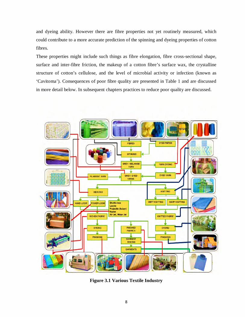
in more detail below. In subsequent chapters practices to reduce poor quality are discussed.
Figure 3.1 Various Textile Industry
9
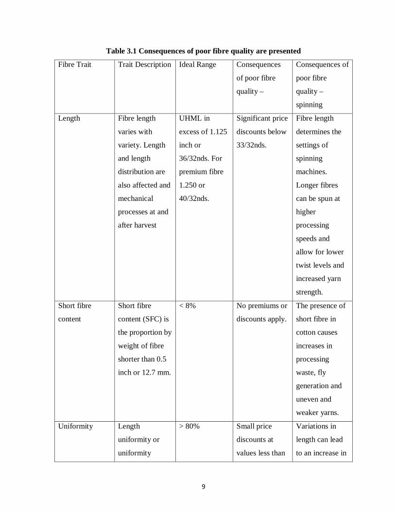
Table 3.1 Consequences of poor fibre quality are presented
Fibre Trait Trait Description Ideal Range Consequences
of poor fibre
quality –
Consequences of
poor fibre
quality –
spinning
Length Fibre length
varies with
variety. Length
and length
distribution are
also affected and
mechanical
processes at and
after harvest
UHML in
excess of 1.125
inch or
36/32nds. For
premium fibre
1.250 or
40/32nds.
Significant price
discounts below
33/32nds.
Fibre length
determines the
settings of
spinning
machines.
Longer fibres
can be spun at
higher
processing
speeds and
allow for lower
twist levels and
increased yarn
strength.
Short fibre
content
Short fibre
content (SFC) is
the proportion by
weight of fibre
shorter than 0.5
inch or 12.7 mm.
< 8% No premiums or
discounts apply.
The presence of
short fibre in
cotton causes
increases in
processing
waste, fly
generation and
uneven and
weaker yarns.
Uniformity Length
uniformity or
uniformity
> 80% Small price
discounts at
values less than
Variations in
length can lead
to an increase in

10
index(UI), is the
ratio between the
mean length and
the UHML
expressed as a
percentage.
78. No
premiums apply.
waste,
deterioration in
processing
performance and
yarn quality
Micronaire Micronaire is a
combination of
fibre linear
density and fibre
maturity. The
test measures the
resistance
offered by a
weighed plug of
fibres in a
chamber of fixed
volume to a
metered airflow.
Micronaire
values between
3.8 and 4.5 are
desirable.
Maturity ratio
>0.85 and
linear density <
220 mtex
Premium range
is considered to
be 3.8 to 4.2
with a linear
density < 180
mtex.
Significant price
discounts below
3.5 and above
5.0.
Linear density
determines the
number of fibres
needed in a yarn
cross-section,
and hence the
yarn count that
can be spun.
Cotton with a
low Micronaire
may have
immature fibre.
High Micronaire
is considered
coarse (high
linear density)
and provides
fewer fibres in
cross section.
Strength The strength of
cotton fibres is
usually defined
as the breaking
force required
for a bundle of
> 29 grams/tex,
small premiums
for values
above 29 /tex.
For premium
fibre> 34
Discounts
appear for
values below 27
g/tex.
The ability of
cotton to
withstand tensile
force is
fundamentally
important in

11
fibres of a given
weight and
fineness
grams/tex.
spinning. Yarn
and fabric
strength
correlates with
fibre strength.
Grade Grade describes
the colour
and‘preparation’
of cotton. Under
this system
colour has
traditionally
been related to
physical cotton
standards
although it is
now measured
with a
colorimeter.
> MID 31,
small premiums
for good
grades.
Significant
discounts for
poor grades.
Aside from
cases of severe
staining the
colour of cotton
and the level of
‘preparation’
have no direct
bearing on
processing
ability.
Significant
differences in
colour can lead
to dyeing
problems.
Trash / dust Trash refers to
plant parts
incorporated
during harvests,
which are then
broken down
into smaller
pieces during
ginning.
Low trash
levels of < 5%
High levels of
trash and the
occurrence of
grass and bark
incur large price
discounts.
Whilst large
trash particles
are easily
removed in the
spinning mill
too much trash
results in
increased waste.
High dust levels
affect open end
spinning

12
efficiency and
product quality.
Bark and grass
are difficult to
separate from
cotton fibre in
the mill because
of their fibrous
nature.
Stickiness Contamination
of cotton from
the exudates of
the silverleaf
whitefly and the
cotton aphid.
Low / none High levels of
contamination
incur significant
price discounts
and can lead to
rejection by the
buyer.
Sugar
contamination
leads to the
build-up of
sticky residues
on textile
machinery,
which affects
yarn evenness
and results in
process
stoppages.
Seed - coat
fragments
In dry crop
conditions seed-
coat fragments
may contribute
to the formation
of a (seed-coat)
nep.
Low / none Moderate price
discounts.
Seed-coat
fragments do not
absorb dye and
appear as‘flecks’
on finished
fabrics.
Neps Neps are fibre
entanglements
that have a hard
< 250
neps/gram. For
premium fibre<
Moderate price
discounts.
Neps typically
absorb less dye
and reflect light

13
central knot.
Harvesting and
ginning affect
the amount of
nep.
200 differently and
appear as light
coloured ‘flecks’
on finished
fabrics.
Contamination Contamination
of cotton by
foreign materials
such as woven
plastic, plastic
film, jute /
hessian, leaves,
feathers, paper
leather, sand,
dust, rust, metal,
grease and oil,
rubber and tar.
Low / none A reputation for
contamination
has a negative
impact on sales
and future
exports.
Contamination
can lead to the
downgrading of
yarn, fabric or
garments to
second quality
or even the total
rejection of an
entire batch.
by stress during fibre development, Fibre length, Length Uniformity, and Short Fibre Content
(SFC). Longer fibres allow finer and stronger yarn to be spun as the twist inserted into longer
fibres traverses and entwines over a longer length of yarn. Fibre length determines the draft
settings of machines in a spinning mill. Longer fibres also mean that less twist needs to be
inserted into yarn, which in turn means production speeds can be increased. Spinning
production is determined by the spinning speed of the spindle, rotor and air current and the
amount of twist required in the yarn. Hence longer fibre allows lower twist levels to be used,
increases yarn strength, improves yarn regularity and allows finer yarn counts to be spun.
Fibre length must stay consistent as variations in length can cause severe problems and lead
to an increase in waste, deterioration in processing performance and yarn quality.
Fibre length is a genetic trait that varies considerably across different cotton species and
varieties. Length and length distribution are also affected by agronomic and environmental
14
factors during fibre development, and mechanical processes at and after harvest. Gin damage
to fibre length is known to be dependent upon variety, seed moisture, temperature (applied in
gin) and the condition of fibre delivered to the gin (e.g. weathered fibre). The distribution
pattern of fibre length in hand-harvested and hand-ginned samples is markedly different from
samples that have been mechanically harvested and ginned; two processes that result in the
breakage of fibres.
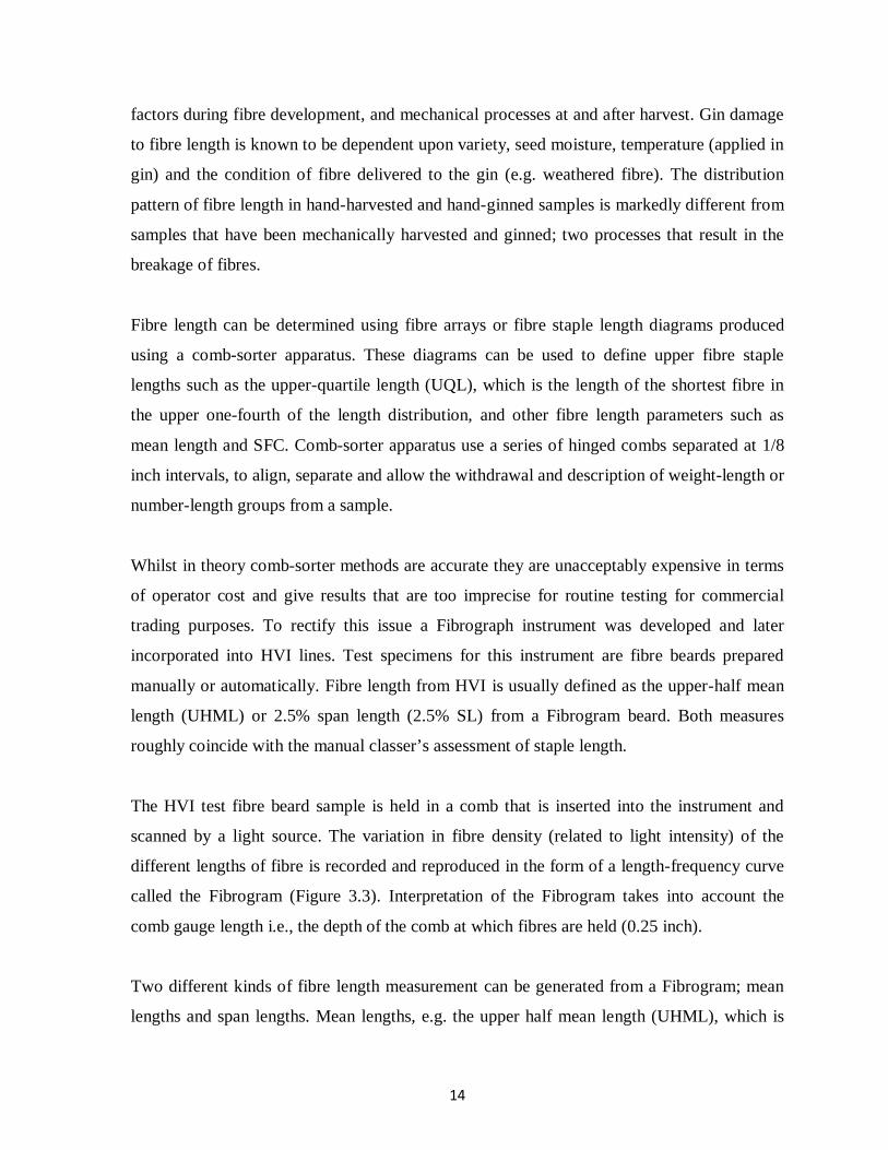
Fibre length can be determined using fibre arrays or fibre staple length diagrams produced
using a comb-sorter apparatus. These diagrams can be used to define upper fibre staple
lengths such as the upper-quartile length (UQL), which is the length of the shortest fibre in
the upper one-fourth of the length distribution, and other fibre length parameters such as
mean length and SFC. Comb-sorter apparatus use a series of hinged combs separated at 1/8
inch intervals, to align, separate and allow the withdrawal and description of weight-length or
number-length groups from a sample.
Whilst in theory comb-sorter methods are accurate they are unacceptably expensive in terms
of operator cost and give results that are too imprecise for routine testing for commercial
trading purposes. To rectify this issue a Fibrograph instrument was developed and later
incorporated into HVI lines. Test specimens for this instrument are fibre beards prepared
manually or automatically. Fibre length from HVI is usually defined as the upper-half mean
length (UHML) or 2.5% span length (2.5% SL) from a Fibrogram beard. Both measures
roughly coincide with the manual classer’s assessment of staple length.
The HVI test fibre beard sample is held in a comb that is inserted into the instrument and
scanned by a light source. The variation in fibre density (related to light intensity) of the
different lengths of fibre is recorded and reproduced in the form of a length-frequency curve
called the Fibrogram (Figure 3.3). Interpretation of the Fibrogram takes into account the
comb gauge length i.e., the depth of the comb at which fibres are held (0.25 inch).
Two different kinds of fibre length measurement can be generated from a Fibrogram; mean
lengths and span lengths. Mean lengths, e.g. the upper half mean length (UHML), which is
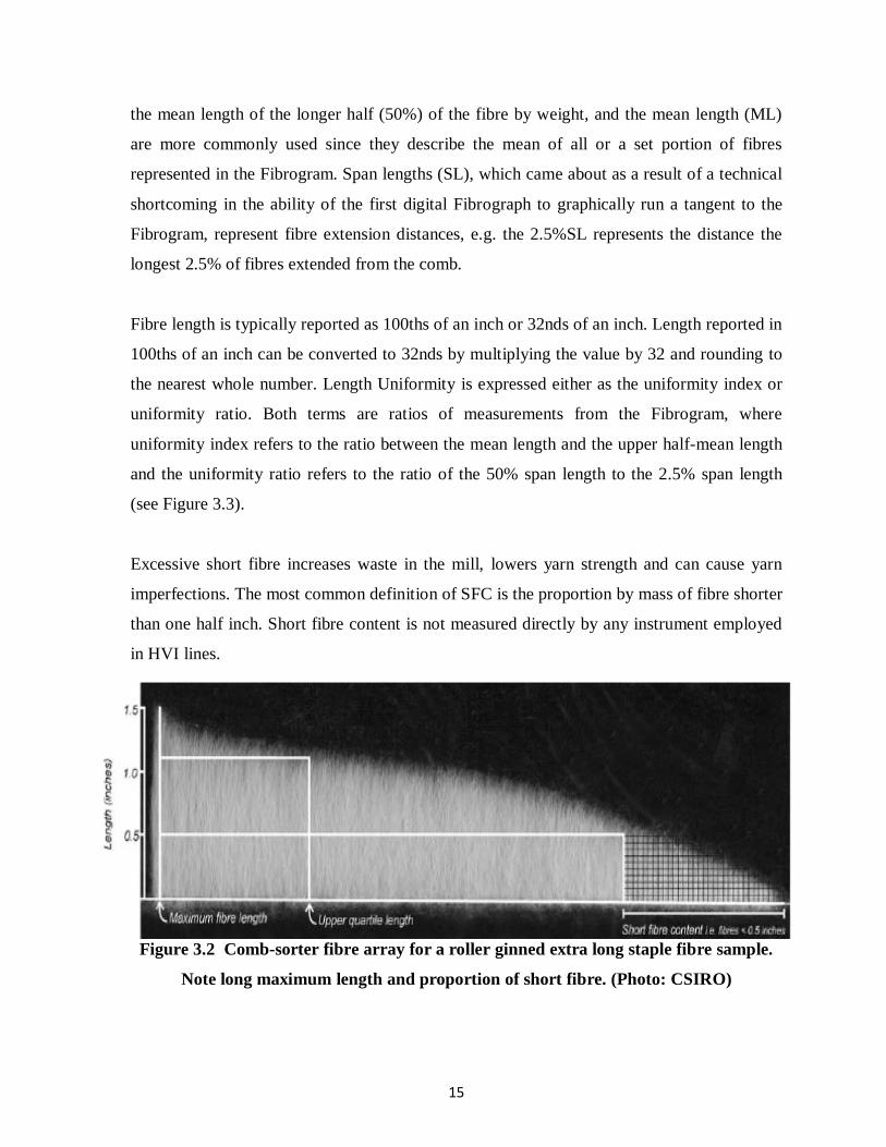
15
the mean length of the longer half (50%) of the fibre by weight, and the mean length (ML)
are more commonly used since they describe the mean of all or a set portion of fibres
represented in the Fibrogram. Span lengths (SL), which came about as a result of a technical
shortcoming in the ability of the first digital Fibrograph to graphically run a tangent to the
Fibrogram, represent fibre extension distances, e.g. the 2.5%SL represents the distance the
longest 2.5% of fibres extended from the comb.
Fibre length is typically reported as 100ths of an inch or 32nds of an inch. Length reported in
100ths of an inch can be converted to 32nds by multiplying the value by 32 and rounding to
the nearest whole number. Length Uniformity is expressed either as the uniformity index or
uniformity ratio. Both terms are ratios of measurements from the Fibrogram, where
uniformity index refers to the ratio between the mean length and the upper half-mean length
and the uniformity ratio refers to the ratio of the 50% span length to the 2.5% span length
(see Figure 3.3).
Excessive short fibre increases waste in the mill, lowers yarn strength and can cause yarn
imperfections. The most common definition of SFC is the proportion by mass of fibre shorter
than one half inch. Short fibre content is not measured directly by any instrument employed
in HVI lines.
Figure 3.2 Comb-sorter fibre array for a roller ginned extra long staple fibre sample.
Note long maximum length and proportion of short fibre. (Photo: CSIRO)
16
Figure 3.3 Typical Fibrogram showing length measurement locations on the fibre
length diagram produced by the Fibrograph.
3.1.1 Fibre strength
Yarn strength is directly related to fibre strength, particularly in rotor spun yarns. Cottons
with good strength can be spun faster and usually result in fewer problems during processing
than weaker cottons. In turn strong yarn improves fabric strength and durability.
Fibre and yarn strength represent the maximum resistance to stretching forces developed
during a tensile test in which a fibre bundle or yarn is broken. The maximum resistance to
these forces is called the breaking load and is measured in terms of grams (or pounds) force.
To account for differences of fibres with different linear densities and for the number of
fibres present in a bundle, the breaking load is adjusted by the number of fibres in the bundle,
which is determined by the linear density of the fibre and the weight of fibre in the bundle.
This adjustment produces the value of tenacity, which is measured in terms of grams
force/tex and allows direct comparison of the strength of different fibres and yarns.
There are also other issues that need consideration when measuring the strength of fibre
bundles (Figure 3.4). One issue relates to the length, known as the gauge length, between the
jaw clamps that hold the fibre bundle. A sample with a high number of short fibres (high

17
SFC) means that many of the fibres may not reach across the gauge length (typically 1/8
inch) to be clamped, resulting in a lower bundle strength measurement. Another important
issue relates to the moisture content of the fibres in the bundle. It is well known that fibre
with high moisture content has a higher strength than ‘dry’ fibre. It is for this reason that
fibre moisture is equilibrated to standard conditions (20°C and 65% relative humidity) before
testing. Fibre tenacity can be increased in excess of 10% by increasing fibre moisture from
5% to 6.5% The effect of fibre maturity or immaturity on fibre bundle strengthtests is also
sometimes a point of contention. Whilst a single mature fibre is inherently stronger than a
single immature fibre by virtue of itscrystalline cellulose structure, this relativity is often not
clearly seen in HVI bundle strength tests. Research has shown that reasonably immature fibre
can still produce good fibre bundle tenacity values and corresponding yarn tenacity values.
The effects seen in this circumstance can probably be attributed to one or a combination of
the following factors. One is inaccurate assessment of fibre linear density and bundle weight
by the HVI and therefore improper adjustment of the fibre bundle/yarn strength value, and
the other is the positive effect of immature fibre having more fibre ends and surface area
contributing to the bundle strength result.
3.1.2 Elongation
Cotton fibre is flexible and can be stretched. The increase in length or deformation of the
fibre before it breaks as a result of stretching is called elongation. Expressed as a % increase
over its original length.
3.1.3 Neps
Neps occur in all ginned cotton but hardly in unpicked seed-cotton. Neps are fibre
entanglements that have a hard central knotthat is detectable (Figure 3.5). Harvesting,
ginning (particularly lint cleaning), opening, cleaning, carding and combing in the mill are
mechanical processes that affect the amount of nep found in cotton. The propensity for cotton
to nep is dependent upon its fibre properties, particularly its linear density and fibre maturity,

18
and the level of biological contamination, e.g. seed coat fragments, bark and stickiness.
Studies have shown generally that over 90% of fibres in a nep are immature.
Figure 3.4 Photo of a fibre array comb for the HVI Fibrograph (length) and strength
tester. (CSIRO).
Figure 3.5 A nep is an entanglement of fibres resulting from mechanical processing.
More neps can occur if cotton is immature. (Photo: CSIRO).
3.1.4 Trash
Trash in seed-cotton is a grower and ginner problem, whilst trash in baled lint is a spinner
problem however, the solutions for the grower and ginner are not always the best solutions
for the spinner. In the gin more cleaning can mean more fibre breakages leading to increased
short fibre content, and more neps. With an increasing number of impurities (i.e. trash), such
as husk, leaf, stalk and seed-coat fragments, the tendency towards inferior yarn quality can

19
increase if the installed opening and cleaning line in a mill is unable to cope with it.
Removing trash is a direct cost to a spinning mill and can cause deterioration in spinning
performance and yarn quality. It is thus imperative for a spinning mill to know what the
cleaning efficiency of its cleaning line is to ensure that it can cope with the trash content in
the cotton lint, especially for rotor and air jet spinning.
3.1.5 Stickiness
Sticky cotton is a major concern for spinning mills. Physiological plant sugars in immature
fibres, contaminants from crushed seedand seed coat fragments, grease, oil and pesticide
residues are all potential sources of stickiness. However, these are insignificant compared
with contamination of cotton from the exudates of the silverleaf whitefly (Bemisiatabaci B-
biotype) and the cotton aphid (Aphis gossypii). The sugar exudates from these insects lead to
significant problems in the spinning mill including a build-up of residues on textile
machinery, which results in irregularities and stoppages in sliver and yarn production. Even
at low to moderately contaminated levels, sugar residues build up, decreasing productivity
and quality, and forcing the spinner to increase the frequency of cleaning schedules. A
reputation for stickiness has a negative impact on sales, exports and price for cotton from
regions suspected of having stickiness.
3.1.6 Colour or grade
Colour is a primary indicator of grade. Discolouration is due a to range of influences
including trash and dust content, rain damage, insect secretions, UV radiation exposure, heat
and microbial decay. Colour in cotton is defined in terms of its reflectance (Rd) and
yellowness (+b), which are measured by a photoelectric cell. Historically grade is a
subjective interpretation of fibre colour, preparation and trash content against ‘official’
standards.

20
3.1.7 Fibre linear density
Fibre linear density (often referred to as fineness) determines the minimum yarn linear
density or yarn count that can be spun from a particular fibre or growth. This is based on the
minimum number of fibres required to physically hold a twisted yarn assembly together. The
linear density of fibres increases with both larger fibre perimeter and greater fibre maturity.
This ‘spin-limit’ minimum will depend ondifferent spinning systems and the level of twist
inserted into the fibre assembly. In general, for ring spinning the minimum numberof cotton
fibres required in the yarn cross-section is around 80(Figure 3.7), for rotor spinning the
number is 100 fibres and for air-jet spinning the number is 75 fibres.
Figure 3.6 The cross section of a cotton yarn showing the packing and interaction of
individual fibres. In this yarn cross-section seventy eight individual fibres are
distinguishable. (Photo: CSIRO).
The linear density of raw cotton used to manufacture a yarn can therefore have a big impact
on yarn evenness. For coarser fibres withhigher linear densities there is a higher probability
of there not being enough fibres in a yarn cross section to support the yarn structure (athin
place) as illustrated below (Figure 3.5). A thin place in a yarn isa weak place, which has
potential to break during either the spinning process itself or later during fabric manufacture.
This can have a significant impact on the efficiency of the spinning process and the effect of
uneven yarn can sometimes be observed in light weight tee shirts or vests where close
21
examination highlights a slightly uneven appearance of the knit structure. So there is
considerable pressure on the spinner to ensure that the yarn manufactured and supplied isas
even as possible so breakages do not occur.
In the example, illustrated in Figure 3.7, imagine if the spinner chose to make the same yarn
from a coarser cotton fibre. In this case, fewer rows of the heavier fibres are required to make
up the required mass for the yarn as shown schematically in Figure. With coarse fibres along
with the natural variation in the number of fibres in the yarn cross-section there are
opportunities for more ‘thin’ places in the yarn cross section.
These effects are well known to the spinner and hence he chooses fibre quality with some
care. The linear density of synthetic fibres is routinely available and fibre diameter (micron)
is used by the wool industry. Spinners carefully use this data to choose appropriate raw
materials for spinning either synthetic or wool yarns. In the case of cotton, unfortunately
fibre linear density is not available to the trade, which instead relies on the Micronaire value
as a proxy for fibre linear density. The Micronaire has limitations as it is unable to properly
distinguish premium fine mature cotton from immature, coarser cotton (smaller fibre
perimeters and lower linear density).
Figure 3.7 Schematic simple representations of the arrangement of fibres within a yarn.
(a) a yarn made with fine fibres (lower linear density) (b) a yarn with a similar linear
density made from coarser fibres (higher linear density). The red line indicates less
fibres in the cross section leading to a thin/weak spot.

22
3.1.8 Micronaire
Micronaire is a measure of the rate at which air flows under pressure through a plug of lint of
known weight compressed into a chamber of fixed volume. The rate of air flow depends on
the resistance offered by the total surface area of the fibres which is related to the linear
density as well as the thickness of the fibre walls. A reduction in linear density, wall
thickness or fibre perimeter decreases the Micronaire reading as there is more fibres in a plug
of cotton that is tested increasing air resistance.
It is important to remember that both yarn count (how fine) and yarn quality (how even and
strong) are the main reasons why fibre linear density is so important, and thus why spinners
prefer to purchase fibres with a specified linear density. Currently, the commercial trade
relies on Micronaire readings to indicate the linear density of cotton, despite it being well
known that the Micronaire readings represent a combination of fibre linear density and fibre
maturity, and as a result is not a particularly accurate measure of either important parameter.
For the spinner there are two potential problems in managing quality using the Micronaire
value. Low Micronaire may indicate the presence of immature fibre and high Micronaire
values may indicate that the cotton is coarse. Instances can occur where Micronaire readings
are similar and fibre traits of fibre maturity and linear density(and wall thickness) can be
entirely different (see Figure3.6). All situations are problematic for the spinner.
Microscope image
Analysed image
Perametric values
Micronaire: 3.1
Linear density: 150 mtex
Theta: 0.41
Perimeter: 56 µm
Wall area: 102 µm2
23
Micronaire: 3.1
Linear density: 81 mtex
Theta: 0.76
Perimeter: 30 µm
Wall area: 56 µm2
Micronaire: 4.3
Linear density: 216 mtex
Theta: 0.43
Perimeter: 65 µm
Wall area: 145 µm2
Micronaire: 4.3
Linear density: 108 mtex
Theta: 0.86
Perimeter: 33 µm
Wall area: 73 µm2
Micronaire: 5.3
Linear density: 279 mtex
Theta: 0.45
Perimeter: 72 µm
Wall area: 187 µm2
Micronaire: 5.3
Linear density: 160 mtex
Theta: 0.78
Perimeter: 42 µm
Wall area: 107 µm2
Figure 3.8 Cross section of fibres that have similar Micronaire values (same surface
area to weight ratios).
For instance, one fibre type achieves a Micronaire of 4.2 because it has a smaller fibre
perimeter (meaning more fibres are present in the plug used for sampling) and has more fibre

24
wall thickening (fibre maturity), overall resulting in a smaller fibre linear density. The other
fibre achieves the same Micronaire as it has a larger fibre perimeter but has poorer fibre wall
thickening (immature) resulting in a larger fibre linear density. (Photo: CSIRO).
3.2 Overview of spinning process
Spinning is the actual process where the yarn is formed. But before spinning can commerce,
fibres must be prepared so that they satisfy the following key requirements:
• The fibres are free from impurities
• The fibres are sufficiently individualised and aligned
• The natural properties of fibres are preserved
• The fibres are prepared in a form that is suitable for feeding the subsequent spinning
process.
Different fibres require different preparation methods. This module discusses the two major
fibre preparation routes - short staple processing and worsted processing. The actual spinning
process is discussed in the next module.
All the important fibre processing stages are covered in this module, including fibre opening
and cleaning, carding, drawing, and combing. In the worsted sector, fibre preparation is
commonly known as top-making. While the details of processing machinery differ in short
staple processing and long staple processing, the basic principle involved is similar.
Preparation of fibres for carpet yarn manufacture (woollen and semi-worsted processing),
and the conversion of manufactured fibres to slivers (Tow-to-sliver conversion) will be
discussed in a separate module.
3.2.1 Short staple processing
Short staple fibres refer to fibres less than 2 inches in length. Cotton is a typical example of
short staple fibre. The short staple system is used to process cotton mainly, cotton/polyester
blends are the next most commonly processed fibres on the short staple system. Other fibres,
such as viscose, are also processed occasionally using the system. Short staple yarns make up
25
the bulk of international yarn market. Since cotton is the dominant fibres used, the emphasis
of this topic will be on cotton processing. The actual spinning of yarns is discussed in a
separate module. At the end of this topic you should be able to:
• Know the flow chart of cotton processing
• Understand the principles and objectives of carding, drawing, and combing
• Appreciate the differences in the process and property of carded ring spun yarn,
combed ring spun yarn, carded rotor spun yarn, and combed rotor spun yarn.
Process overview
The process flow chart for cotton processing from fibre to yarn is shown in Figure 3.9.
Figure 3.9. Fibre to yarn processing for cotton
B low -room processes (ble nd, open & c lea n)
C arding
Draw ing
Lap forming
Combing
D raw ing (x 2)
R otor spinning Roving
R ing spinning
S hort staple yarns Carde d roto r spun yarn, Carde d ring spu n yarn Com bed rotor sp un yarn, Com bed ring spu n yarn
C otton growing
Ginning
C OTTON LINT
(Transpo rt to text ile m ill)
Ba ling, H VI C lass ing
Enginee re d Fibre Selec t ion EFS
(M arsh alling into “m ixes ” or laydo wns)
Cotton see d - by produc t
Agricu ltural P rocesses
Textile Processes
Harves t

26
The agricultural processes include cotton growing, harvesting and ginning. Cotton grown in
different regions have different properties. Modern cotton harvesting uses machine pickers or
strippers. Since cotton fibres do not mature at the same time and machine picking is less
discriminative than traditional hand picking, large quantities of impurities such as green
bolls, leaf, stick, and trash are also picked up during cotton harvesting, together with the seed
cotton. On a weight basis, “seed cotton” contains approximately 35% fibre (lint), 55% seed,
and 10% trash. Obviously the cotton seed and other impurities need to be removed from the
fibres. This is largely done in a gin, which removes all green balls and cotton seeds, about
95% burrs, 92% sticks, and about 85% fine trash. The actual process (in a gin) that separates
cotton fibres and the seed they grow attached to is called ginning. Other machines are also
used before and after ginning to mechanically clean the fibres. The ginned cotton is now
known as cotton lint or lint cotton. The fibres in the cotton lint vary considerably in length
because of fibre breakage caused by the severe mechanical actions during ginning and
cleaning. The cotton lint is then sampled and packed into bales weighing 227 kg (or 500
pounds), containing over 60 billion individual fibres. The reading material "latest moves in
cotton ginning" by Audas (1994) provides essential details on the ginning process.
Fibre samples are now tested on the High Volume Instrument (HVI) for a range of fibre
properties, including strength, elongation, length, uniformity, micronaire, colour, and trash.
The HVI system was developed in the late 1960s and has been increasingly accepted since
the 1980s. Before the introduction of the HVI system, cotton in a bale was graded
subjectively by experienced cotton classers for properties such as staple length, colour, and
trash content. The results were then used to assign cotton bales into lots or categories. When
the cotton was ready for consumption, the bales were grouped into mixes or laydowns. Bales
from different regions were mixed in proportion to the number of bales in each lot and fed
into the opening line machinery in the blow-room.
Today, objective measurement is widely used. When the bales arrive at a textile mill to start
the textile processes, the test results are used as a basis for fibre selection and mixing
according to the end product requirements. The modern cotton mill will "engineer" its yarn to
meet specific end-use requirements. The engineered fibre selection (EFS) system, introduced
27
by Cotton Inc. (USA) in 1982, has been used increasingly by cotton mills to facilitate this
important task. It is most useful in bale management, particularly for storing and retrieving
bales, for selecting bales with fibre properties within specified ranges and average values, for
composing consistent bale laydowns and for predicting yarn strength and other yarn
properties based on tailer-made regression analyses.The bulk of the cotton bales consumed in
America is now managed at the mill level by the engineered fibre selection system (EFS).
More information on EFS is available from Cotton Inc.'s web site
(http://www.cottoninc.com).
Adequate fibre blending and mixing is also vital to ensure processing efficiency and yarn
quality. The cotton lint still contains some small trash particles, which have to be removed by
the textile processes, such as carding and combing. The textile processes also perform fibre
opening, fibre alignment, fibre mixing and attenuation to get the fibres ready for spinning.
Depending on the particular processing route followed, four major types of cotton yarn may
be produced – carded rotor spun, carded ring spun, combed rotor spun, combed ring spun. An
overview of the key stages is given in Table 3.2
Table 3.2 Overview of cotton growing, ginning and yarn manufacturing stages
Cotton Growing Cotton Ginning Cotton Yarn Manufacture
Planting of selected cotton
varieties (eg. Siokra L23)
Fertilising and irrigation
Weed and insect control
Application of growth
regulators
Application of harvesting
aids (eg. defoliants)
Single harvest by spindle
harvester or stripper
Removal or green bolls, sticks
etc
Separation of lint from seed
Lint cleaning (up to 3 stages)
Sampling and baling
Weighing and testing
(classing)
Storage and transport to
spinning mill
Selection of bale laydowns or
mixes
Blowroom processes
Carding
Drawing
Combing (if necessary)
Further drawing
Spinning (ring, rotor or air-
jet)

28
It is important to keep in mind at this stage that before fibres can be made into useful yarns,
they should be:
• Free from impurities
• Well individualised and aligned
• Well mixed
• Of adequate length and strength
Knowing these requirements will help us understand why the fibres need to go through many
textile processes before the actual spinning process. For instance, in order to remove
impurities imbedded in fibres, we need to open the fibres first to expose those impurities.
Fibre opening needs to be gradually carried out so as not to stress and damage the fibres too
much. In fact, there are two opening stages:
Stage 1: Breaking apart (break large tufts of fibres into small tufts)
Stage 2: Opening out (open small tufts into individual fibres)
Individualising the fibres is very important. As mentioned in the module on yarn evenness,
poorly separated fibres will travel in groups during drafting, which will lead to reduced
evenness and increased imperfections in the final yarn. For a yarn to have adequate strength,
fibres in the yarn should be well aligned in order to share the applied load on the yarn. The
different degrees of fibre alignment in different yarns often explain the differences in yarn
properties. Because of the variability that exists both within and between fibres, fibres should
be well mixed before the actual spinning stage. There are two basic requirements for a good
fibre mix or blend: Requirement 1: The blend (mix) is homogenous & requirement 2: The
blend (mix) is intimate
The first requirement entails that different fibres are mixed in the right proportion, while the
second requirement can only be achieved with different individual fibres lying side by side.
Preserving the quality of fibres during processing is also essential to ensure yarn quality.
Damage to fibre length and strength will lead to reduced yarn strength. With this overall
picture in mind, we can now discuss the individual textile processes applied to fibres.

29
FW
Wt
FW
FW
FW
WF
n
n
tb
.....2
2
1
1
3.2.2 The blowroom processes
The blowroom is the section of a cotton spinning mill where the preparatory processes of
opening, blending and cleaning are carried out. The blowroom machines blend, open and
clean the ginned cotton before feeding it to the cotton card.
The ginned cotton, still contaminated with some impurities, arrives in the textile mill in
compressed bales, fibre properties often vary from bale to bale. Blending is regarded as the
most important process in a cotton spinning mill. It reduces variation of fibre characteristics,
permits uniform processing and improves yarn quality. In the blending process, different
cottons of known physical properties are combined to give a mix with the required or pre-
determined average characteristics. For example, the general formula for calculating the
theoretical fineness (micronaire, μg/in.) is as follows
----------------(1)
Where Fb is the fineness of a blend of n components; Wt is the total weight of the blend; and
W is the weight of any one component and F is its fineness. In terms of weight percentages,
the above equation becomes:
-------------------(2)
Principle of Fiber to yarn conversion systems
•Convert a high variable raw material to a very consistent fiber strand.
•Variability exists Within bales, Between bales within one mix, and Between mixes (lay
downs).
•Quality criteria is high degree of uniformity, consistent properties along the yarn.
•fibers are normally intermingled with all kinds of trash, dust, seed coat fragments,…
•The yarn produced must be pure, clean and defect free and high efficiency.
FP
FP
FP
FPF
n
nb
100
.....
100
2
2
1
1

30
3.10 Flow chart Cotton Ring Spinning
Figure 3.10 Flow chart Cotton Ring Spinning
3.2.3 Blowing room
Short Staple Pre-Spinning Machinery
•All Modern Spinning mills are equipped by some sort of Automatic Bale Opener .
•In General short lines, does not need material handling, and hence less reliable for faults.
•Short staple pre-spinning emphasized compact lines with integrated multi- functional
equipment.
•Major emphases were placed upon equipment allowing for a compact 800 Kg/hr opening
line, an integrated separator, a more precise removal of foreign fibers, and a waste control
measuring system.

31
3.2.4 Rieter opening line The main task of opening room is to open the big flocks to small tufts, cleaning i.e. trash
removing, fiber mixing and even feed for carding machine.
Figure 3.11 : Rieter VarioSet Blowing room/Carding room
Figure 3.12. Trutschler Modular Opening Component Line
The Different machines comprising the opining line are multi functional
• New features are installed such foreign matter separator to prevent mixing of different
fibers in the blend
• Completely automated and computerized control, vision system is enabled on-line

32
Blending Bale Opener working width of 1720 mm and a machine length of 50 m, about 130
bales can be accommodated (one or two sided). The BLENDOMAT with a working width of
2300 mm even accommodates up to 180 bales. Assuming a cleaning line production rate of
800 kg/h, this allows unattended operation for two days (48 h).
3.2.5 Waste opener
Process waste with high fiber content (usually from the intermediate process to spinning, up-
stream of the blowroom) may be recycled by feeding into the process line around 5% of
waste with the virgin fiber. Since the waste is usually made up of fibers that have previously
passed through the blowroom, it is important to keep further mechanical treatment to a
minimum, so as to reduce fiber breakage.
Multi-function separator SP-Mf ( heavy particle detection and extraction) do the following:
1 The material is sucked off an automatic bale opener
2 Fan automatically control the constant negative pressure
3 A new guiding profile for the aerodynamic heavy particle separator 4 The spark sensor
detects burning material
5 In the air flow separator the dusty air is separated
6 metal detector detects any kind of metals
7 The diverter is actively opened and closed
8 fan in front of the mixer, sucks the material off here.
9 A flap feeds the separated heavy particles
10 The two waste containers are large-size
11 A fire extinguishing unit extinguishes the burning material in the waste container
12 A heat sensor monitors the waste container for fire
13 The dusty exhaust air
14 Opened waste

33
3.2.6 Blending/mixing
The direct feeding of a cleaner of the CLEANOMAT system by an integrated mixer MX-I is
an important element of the compact blow room. This mixer produces a homogeneous and
even web for feeding the cleaner. The air separation at the mixer provides additional dust
removal. This combination of a cleaner with a mixer is the solution which ensures the
greatest savings in floor space and energy and is the preferred solution when processing
cotton.
3.2.7 Optimum setting of cleaning
Gentle opening is achieved by having the first beater clothed in pins angled ca. 10∞from the
vertical, and the remaining beaters having saw-tooth clothing, the tooth angle increasing from
roller to roller (e.g. 15∞, 30∞, 40∞). The teeth density (number of points per cm2) should
also progressively increase from beater 1 to 4, depending on fineness of the fiber being
produced. Importantly, the beater speeds should progressively increase from beater 1 to 4
(for example 300, 500, 800, 1200, rmin–1).
Hence, the mean tuft size is decreased (approximate figures) from 1 mg by the first beater to
0.7 mg, 0.5 mg and 0.1 mg by the second, third and fourth beaters, respectively. It is only the
fourth beater that reaches a sufficiently high surface speed at which the finest trash particles
are ejected.
3.2.8 Basic actions in carding
There are two basic actions in cotton carding: carding (or working) action and stripping
action. The tooth direction and relative surface speed decide which action occurs between
two adjacent and clothed (or toothed) surfaces.
Each tooth has a point and a back, as indicated in figure 3.13a.
If the tip of the tooth on one surface points to the tip of the tooth on the other surface, a point-
to-point carding (or working) action occurs (figure 3.13b).
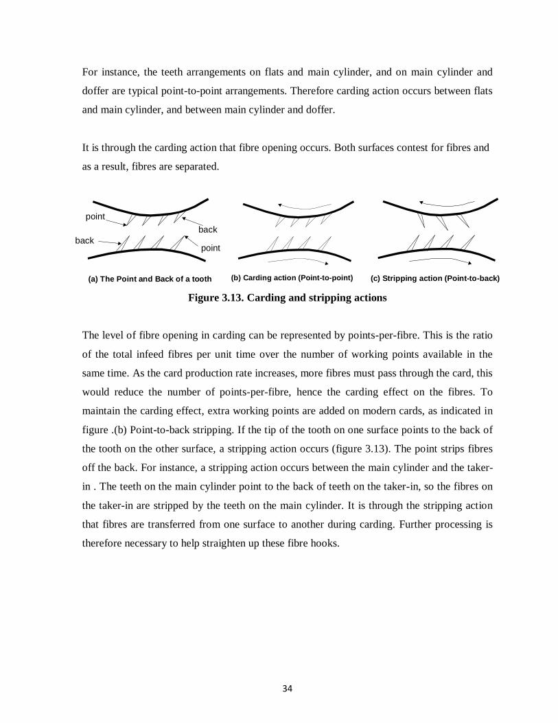
34
For instance, the teeth arrangements on flats and main cylinder, and on main cylinder and
doffer are typical point-to-point arrangements. Therefore carding action occurs between flats
and main cylinder, and between main cylinder and doffer.
It is through the carding action that fibre opening occurs. Both surfaces contest for fibres and
as a result, fibres are separated.
Figure 3.13. Carding and stripping actions
The level of fibre opening in carding can be represented by points-per-fibre. This is the ratio
of the total infeed fibres per unit time over the number of working points available in the
same time. As the card production rate increases, more fibres must pass through the card, this
would reduce the number of points-per-fibre, hence the carding effect on the fibres. To
maintain the carding effect, extra working points are added on modern cards, as indicated in
figure .(b) Point-to-back stripping. If the tip of the tooth on one surface points to the back of
the tooth on the other surface, a stripping action occurs (figure 3.13). The point strips fibres
off the back. For instance, a stripping action occurs between the main cylinder and the taker-
in . The teeth on the main cylinder point to the back of teeth on the taker-in, so the fibres on
the taker-in are stripped by the teeth on the main cylinder. It is through the stripping action
that fibres are transferred from one surface to another during carding. Further processing is
therefore necessary to help straighten up these fibre hooks.
(b) Carding action (Point-to-point) (c) Stripping action (Point-to-back) (a) The Point and Back of a tooth
back back
point
point

35
3.2.9 Drawing
Converting bales of fibres to a thin strand of fibres or yarns requires enormous fibre
attenuation. Put simply, attenuation (drafting) is to make input material longer and thinner.
In this sense, carding can also be regarded as a fibre attenuation process. Drawing continues
the fibre attenuation, it also performs several other functions.
Objectives
The drawing process aims at achieving the following objectives:
• Attenuate the card slivers
• Reduce the fibre hooks and improve fibre alignment
• Blend and mix fibres
• Reduce the irregularity of card slivers by doubling
Drawing usually implies the actions of doubling and drafting. Doubling is the combing of
several slivers and drafting is attenuation.
By now we already know that fibres in card slivers are by no means straight and parallel, and
there are many hooked fibres, particularly trailing hooks, in the card slivers. Many of these
hooks should be straightened as fibres slide past each other in the drawing process. Slivers
from different cards vary evenness and other properties, and should be blended to reduce the
irregularity. Cotton and synthetics are often blended in drawing in sliver form. Finally, when
card slivers are combined (doubled), attenuation is necessary to reduce the thickness of the
drawn sliver. Drawing plays a crucial role in the final quality of yarn, and a good
understanding of the fundamentals of drawing is essential.
The material draft and mechanical draft are not always equal. The material draft is the real
draft. The ratch is also known as the ratch length or ratch setting. It is set according to the
length of the longest fibres in order to prevent these fibres from being stretched to break. The
main aim of fibre control is to keep the floating fibres at the speed of back rollers until they
reach the front roller nip (i.e. to prevent fibres being accelerated out of turn), while still
allowing long fibres to be drafted. Different yarn manufacture systems, and different process
in the same system, often apply different control device in drafting.
36
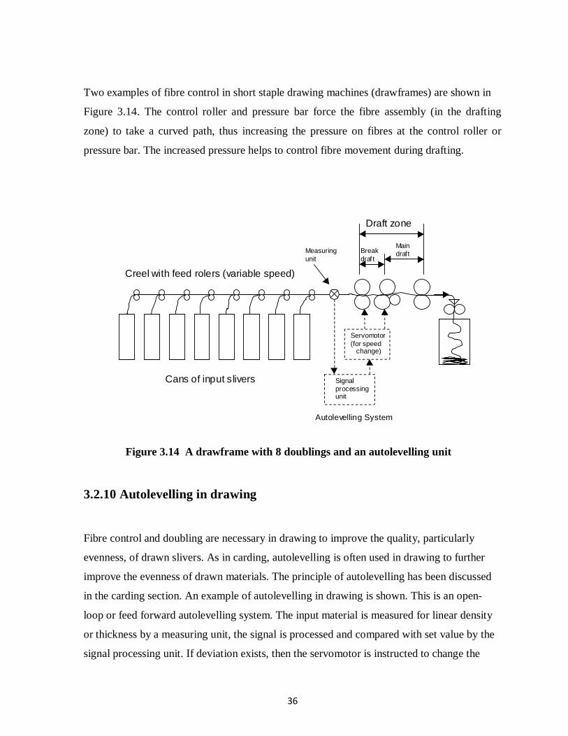
Two examples of fibre control in short staple drawing machines (drawframes) are shown in
Figure 3.14. The control roller and pressure bar force the fibre assembly (in the drafting
zone) to take a curved path, thus increasing the pressure on fibres at the control roller or
pressure bar. The increased pressure helps to control fibre movement during drafting.
Figure 3.14 A drawframe with 8 doublings and an autolevelling unit
3.2.10 Autolevelling in drawing
Fibre control and doubling are necessary in drawing to improve the quality, particularly
evenness, of drawn slivers. As in carding, autolevelling is often used in drawing to further
improve the evenness of drawn materials. The principle of autolevelling has been discussed
in the carding section. An example of autolevelling in drawing is shown. This is an open-
loop or feed forward autolevelling system. The input material is measured for linear density
or thickness by a measuring unit, the signal is processed and compared with set value by the
signal processing unit. If deviation exists, then the servomotor is instructed to change the
Draft zone
Main draft Measuring
unit
Signal processing unit
Servomotor (for speed change)
Creel with feed rolers (variable speed)
Autolevelling System
Cans of input slivers
Break draf t

37
speed of the drafting rollers to adjust the draft in other to reduce the irregularity of the output
material.
3.2.10.1 Fibre straightening in drawing
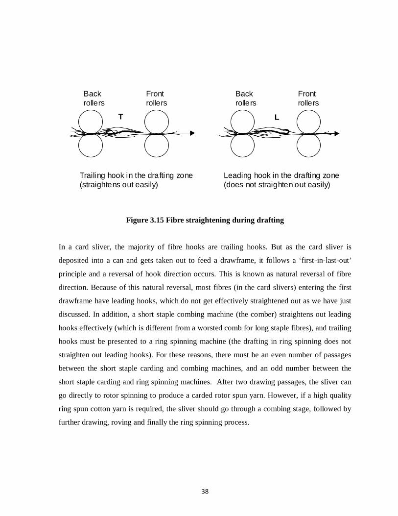
We already know that most fibres in card slivers are hooked fibres, and one of the key
objectives of drawing is to straighten out these hooked fibres. Consider a trailing hook (T)
and a leading hook (L) in drawing as shown in Figure 3.15. For the trailing hook, it will
travel initially at the speed of the back drafting rollers. Soon its leading end, embedded in
‘fast-moving’ fibres under the influence of the front drafting rollers, will travel with the ‘fast-
moving’ fibres at the front roller speed. Since the hooked end of the fibre is still embedded in
a relatively thick body of ‘slow-moving’ fibres controlled by the back rollers, the difference
in speed between the leading end and trailing (hooked) end will straighten out the hook. For
the fibre with leading hook (L), the hook can get caught easily by the ‘fast moving’ fibres
and travel at the front roller speed, while the unhooked trailing end offers little resistance to
its acceleration. As a result, the leading hook (L) is likely to persist into the output material.
From this brief discussion, it is clear that one passage through a drawframe only effectively
removes trailing hooks.
M easu r in gu n i t
R e gu l a to ru n it
C o n tro lu n it
R e f.S ig n a l
M ate r ia lin p u t
M a te r ia lo u tp u t
A n o pen-loo p (feed-forw ard) co ntro lsystem
38
Figure 3.15 Fibre straightening during drafting
In a card sliver, the majority of fibre hooks are trailing hooks. But as the card sliver is
deposited into a can and gets taken out to feed a drawframe, it follows a ‘first-in-last-out’
principle and a reversal of hook direction occurs. This is known as natural reversal of fibre
direction. Because of this natural reversal, most fibres (in the card slivers) entering the first
drawframe have leading hooks, which do not get effectively straightened out as we have just
discussed. In addition, a short staple combing machine (the comber) straightens out leading
hooks effectively (which is different from a worsted comb for long staple fibres), and trailing
hooks must be presented to a ring spinning machine (the drafting in ring spinning does not
straighten out leading hooks). For these reasons, there must be an even number of passages
between the short staple carding and combing machines, and an odd number between the
short staple carding and ring spinning machines. After two drawing passages, the sliver can
go directly to rotor spinning to produce a carded rotor spun yarn. However, if a high quality
ring spun cotton yarn is required, the sliver should go through a combing stage, followed by
further drawing, roving and finally the ring spinning process.
Front rollers
Back rollers
Front rollers
Back rollers
T L
Trailing hook in the drafting zone (straightens out easily)
Leading hook in the drafting zone (does not straighten out easily)
39
3.2.11 Roving
A roving is a fine strand (slubbing) intended to be fed into the ring spinning machines (ring
frames) for making yarns. Rotor spinning machine and other new spinning systems use
slivers as feed materials. But conventional ring frames still use rovings as the feed material.
A roving is much thinner than a sliver, but thicker than a yarn.
The main objective of the roving machine is to further attenuate the drawn sliver (to make it
longer and thinner) and get it ready for spinning. The draw frame has already produced a
sliver that is clean, and consists of more or less parallel fibres. Such a sliver satisfies the
essential requirements for yarn production. The question is why is there a need for the roving
process and why can’t we feed slivers to conventional ring frames? There are two major
reasons for this need. First, a very high draft, in the order of 300 to 500, is required to bring
the thickness of a sliver into the thickness of a yarn. Conventional ring frames can not cope
with such a high draft. Second, the drawframe slivers are deposited in bulky sliver cans,
which are difficult to transport and present to the ring frames as feed material. The much
smaller roving packages are better suited for the purpose.
The commonly used roving machine for cotton is a flyer frame (or speed frame) as shown in
Figure 3.16 . There are three basic steps in the operation of the roving frame – drafting,
twisting, and winding. These basic steps are exactly the same as the basic steps required in
spinning. Consequently, an understanding of the roving process will help us understand the
spinning process to be discussed in the next module.The input to this roving frame is a drawn
sliver (either carded or combed) from the last drawing process. The sliver is drafted by a
roller drafting unit. Between the front and back rollers (the drafting zone), the fibres pass
between the double aprons, which control the fibre movement during drafting. The front nose
of the double aprons is set close to the front roller nip for good drafting performance. You
may recall the concept of perfect roller drafting, which requires that fibres in the drafting
zone travel at the speed of back rollers until the fibre leading ends reach the front roller nip.
The double aprons travel at about the same speed as the back rollers, and they control the
fibres until they reach the front roller nip. A small amount of twist (30 to 65 turns per meter)
is inserted into the drafted fibre strand via the rotation of the flyer. The bobbin (on a spindle)
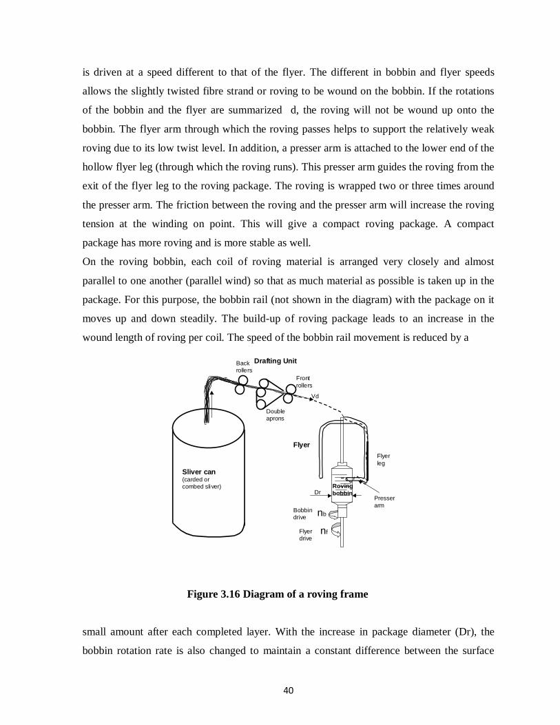
40
is driven at a speed different to that of the flyer. The different in bobbin and flyer speeds
allows the slightly twisted fibre strand or roving to be wound on the bobbin. If the rotations
of the bobbin and the flyer are summarized d, the roving will not be wound up onto the
bobbin. The flyer arm through which the roving passes helps to support the relatively weak
roving due to its low twist level. In addition, a presser arm is attached to the lower end of the
hollow flyer leg (through which the roving runs). This presser arm guides the roving from the
exit of the flyer leg to the roving package. The roving is wrapped two or three times around
the presser arm. The friction between the roving and the presser arm will increase the roving
tension at the winding on point. This will give a compact roving package. A compact
package has more roving and is more stable as well.
On the roving bobbin, each coil of roving material is arranged very closely and almost
parallel to one another (parallel wind) so that as much material as possible is taken up in the
package. For this purpose, the bobbin rail (not shown in the diagram) with the package on it
moves up and down steadily. The build-up of roving package leads to an increase in the
wound length of roving per coil. The speed of the bobbin rail movement is reduced by a
Figure 3.16 Diagram of a roving frame
small amount after each completed layer. With the increase in package diameter (Dr), the
bobbin rotation rate is also changed to maintain a constant difference between the surface
Sliver can (carded or combed sliver)
Drafting Unit
Flyer
Vd
nf
nb
Dr Roving bobbin
Flyer leg
Presser arm
Front rollers
Double aprons
Back rollers
Bobbin drive
Flyer drive
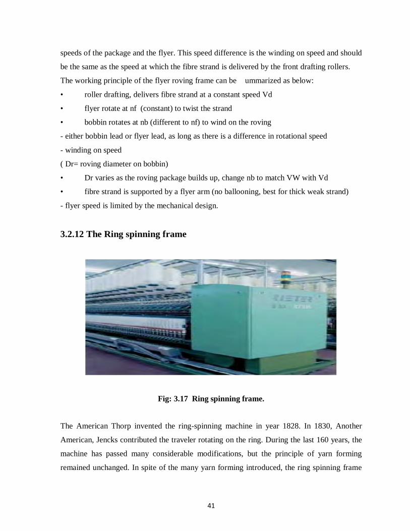
41
speeds of the package and the flyer. This speed difference is the winding on speed and should
be the same as the speed at which the fibre strand is delivered by the front drafting rollers.
The working principle of the flyer roving frame can be ummarized as below:
• roller drafting, delivers fibre strand at a constant speed Vd
• flyer rotate at nf (constant) to twist the strand
• bobbin rotates at nb (different to nf) to wind on the roving
- either bobbin lead or flyer lead, as long as there is a difference in rotational speed
- winding on speed
( Dr= roving diameter on bobbin)
• Dr varies as the roving package builds up, change nb to match VW with Vd
• fibre strand is supported by a flyer arm (no ballooning, best for thick weak strand)
- flyer speed is limited by the mechanical design.
3.2.12 The Ring spinning frame
Fig: 3.17 Ring spinning frame.
The American Thorp invented the ring-spinning machine in year 1828. In 1830, Another
American, Jencks contributed the traveler rotating on the ring. During the last 160 years, the
machine has passed many considerable modifications, but the principle of yarn forming
remained unchanged. In spite of the many yarn forming introduced, the ring spinning frame

42
will continue for some time for the following reasons: It is universally applicable, i. e.
processes any material for any count, quantities.
•It delivers a yarn with optimal characteristics (regarding structure and properties).
•It is uncomplicated and easy to master,
•The know-how for operation is well established and friendly use.
•It is flexible as regards (blend and lot size.)
Basic Principle of Spinning:
•Drafting mechanism
•Consolidation mechanism
•Winding and package forming mechanism.
The ring spinning is characterized by two main features:
1) Continuity of fiber flow roving to yarn.
2) Tension-controlled spinning process.
43
CHAPTER 4
FUZZY LOGIC
4.1 Introduction
Proposed by Lotfi A Zadeh [18] in 1965, Fuzzy logic is an extension of the classical
propositional and predicate logic that rests on the principles of the binary truth functionality.
Fuzzy logic is all about the relative importance of precision. As complexity rises, precise
statements lose meaning and meaningful statements lose precision.
Fuzzy logic is a fascinating area of research because it does a good job of trading off between
significance and precision — something that humans have been managing for a very long
time. Fuzzy logic sometimes appears exotic or intimidating to those unfamiliar with it, but
once you become acquainted with it, it seems almost surprising that no one attempted it
sooner. In this sense fuzzy logic is both old and new because, although the modern and
methodical science of fuzzy logic is still young, the concepts of fuzzy logic reach right down
to our bones. Fuzzy logic is a convenient way to map an input space to an output space. This
is the starting point for everything else, and the great emphasis here is on the word
“convenient.”
4.2 Difference of fuzzy logic from conventional control methods
Fuzzy Logic incorporates a simple, rule-based IF X AND Y THEN Z approach to a solving
control problem rather than attempting to model a system mathematically. The FL model is
empirically-based, relying on an operator’s experience rather than their technical
understanding of the system. For example, rather than dealing with temperature control in
terms such as “SP=500F”, “T <1000F”, or “210C <TEMP <220C”, terms like “IF (process is
too cool) AND (process is getting colder) THEN (add heat to the process)” or “IF (process is
too hot) AND (process is heating rapidly) THEN (cool the process quickly)” are used. These
terms are imprecise and yet very descriptive of what must actually happen. Consider what
you do in the shower if the temperature is too cold: you will make the water comfortable very
quickly with little trouble. FL is capable of mimicking this type of behavior but at very high
rate.
44
4.3 Use of fuzzy logic
Here is a list of general observations about fuzzy logic:
•Fuzzy logic is conceptually easy to understand. The mathematical concepts behind fuzzy
reasoning are very simple. What makes fuzzy nice is the “naturalness” of its approach and
not its far-reaching complexity.
•Fuzzy logic is flexible. With any given system, it’s easy to massage it or layer more
functionality on top of it without starting again from scratch.
•Fuzzy logic is tolerant of imprecise data. Everything is imprecise if you look closely
enough, but more than that, most things are imprecise even on careful inspection. Fuzzy
reasoning builds this understanding into the process rather than tacking it onto the end.
•Fuzzy logic can model nonlinear functions of arbitrary complexity.
You can create a fuzzy system to match any set of input-output data. This process is made
particularly easy by adaptive techniques like ANFIS (Adaptive Neuro-Fuzzy Inference
Systems), which are available in the Fuzzy Logic Toolbox.
•Fuzzy logic can be built on top of the experience of experts. In direct contrast to neural
networks, which take training data and generate opaque, impenetrable models, fuzzy logic
lets you rely on the experience of people who already understand your system.
•Fuzzy logic can be blended with conventional control techniques. Fuzzy systems don’t
necessarily replace conventional control methods. In many cases fuzzy systems augment
them and simplify their implementation.
•Fuzzy logic is based on natural language.
The basis for fuzzy logic is the basis for human communication. This observation underpins
many of the other statements about fuzzy logic. The last statement is perhaps the most
important one and deserves more discussion. Natural language, that which is used by
ordinary people on a daily basis, has been shaped by thousands of years of human history to
be convenient and efficient. Sentences written in ordinary language represent a triumph of
efficient communication. We are generally unaware of this because ordinary language is, of
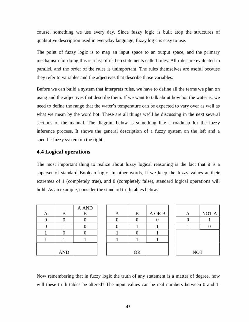
45
course, something we use every day. Since fuzzy logic is built atop the structures of
qualitative description used in everyday language, fuzzy logic is easy to use.
The point of fuzzy logic is to map an input space to an output space, and the primary
mechanism for doing this is a list of if-then statements called rules. All rules are evaluated in
parallel, and the order of the rules is unimportant. The rules themselves are useful because
they refer to variables and the adjectives that describe those variables.
Before we can build a system that interprets rules, we have to define all the terms we plan on
using and the adjectives that describe them. If we want to talk about how hot the water is, we
need to define the range that the water’s temperature can be expected to vary over as well as
what we mean by the word hot. These are all things we’ll be discussing in the next several
sections of the manual. The diagram below is something like a roadmap for the fuzzy
inference process. It shows the general description of a fuzzy system on the left and a
specific fuzzy system on the right.
4.4 Logical operations
The most important thing to realize about fuzzy logical reasoning is the fact that it is a
superset of standard Boolean logic. In other words, if we keep the fuzzy values at their
extremes of 1 (completely true), and 0 (completely false), standard logical operations will
hold. As an example, consider the standard truth tables below.
A B A AND
B A B A OR B A NOT A 0 0 0 0 0 0 0 1 0 1 0 0 1 1 1 0 1 0 0 1 0 1 1 1 1 1 1 1 AND OR NOT
Now remembering that in fuzzy logic the truth of any statement is a matter of degree, how
will these truth tables be altered? The input values can be real numbers between 0 and 1.

46
What function will preserve the results of the AND truth table (for example) and also extend
to all real numbers between 0 and 1? One answer is the min operation. That is, resolve the
statement A AND B, where A and B are limited to the range (0,1), by using the function
min(A,B). Using the same reasoning, we can replace the OR operation with the max
function, so that A OR B becomes equivalent to max (A, B). Finally, the operation NOT A
becomes equivalent to the operation 1 – A. Notice how the truth table above is completely
unchanged by this substitution.
A B MIN(A,B) A B MAX(A,B) A 1-A 0 0 0 0 0 0 0 1 0 1 0 0 1 1 1 0 1 0 0 1 0 1 1 1 1 1 1 1 AND OR NOT
4.5 Fuzzy subset
There is a strong relationship between Boolean logic and the concept of a subset. There is a
similar strong relationship between fuzzy logic and fuzzy subset theory.
A subset U of a set S can be defined as a set of ordered pairs, each with a first element that is
an element of the set S, and a second element that is an element of the set { 0, 1 }, with
exactly one ordered pair present for each element of S. This defines a mapping between
elements of S and elements of the set {0, 1}. The value zero is used to represent non-
membership, and the value one is used to represent membership. The truth or falsity of the
statement x is in U is determined by finding the ordered pair whose first element is x. The
statement is true if the second element of the ordered pair is 1, and the statement is false if it
is 0.
Similarly, a fuzzy subset F of a set S can be defined as a set of ordered pairs, each with a first
element that is an element of the set S, and a second element that is a value in the interval [0,

47
1], with exactly one ordered pair present for each element of S. This defines a mapping
between elements of the set S and values in the interval [0, 1]. The value zero is used to
represent complete non-membership, the value one is used to represent complete
membership, and values in between are used to represent intermediate degrees of
membership. The set S is referred to as the universe of discourse for the fuzzy subset F.
Frequently, the mapping is described as a function, the membership function of F. The
degree to which the statement x is in F is true is determined by finding the ordered pair
whose first element is x. The _degree of truth_ of the statement is the second element of the
ordered pair.
4.5.1 Logic operations
Ok, we now know what a statement like X is LOW means in fuzzy logic. The question now
arises, how do we interpret a statement like X is LOW and Y is HIGH or (not Z is
MEDIUM) The standard definitions in fuzzy logic are: truth (not x) = 1.0 – truth (x) ruth (x
and y) = minimum (truth(x), truth(y)) truth (x or y) = maximum (truth(x), truth(y)) which are
simple enough. Some researchers in fuzzy logic have explored the use of other interpretations
of the AND and OR operations, but the definition for the NOT operation seems to be safe.
Note that if you plug just the values zero and one into these definitions, you get the same
truth tables as you would expect from conventional Boolean logic.
4.6 Defuzzification
Sometimes it is useful to just examine the fuzzy subsets that are the result of the composition
process, but more often, this fuzzy value needs to be converted to a single number a crisp
value. This is what the defuzzification sub process does.
There are more defuzzification methods than you can shake a stick at. A couple of years ago,
Mizumoto (17) did a short paper that compared roughly thirty defuzzification methods. Two
of the more common techniques are the CENTROID and MAXIMUM methods. In the
CENTROID method, the crisp value of the output variable is computed by finding the
variable value of the center of gravity of the membership function for the fuzzy value. In the
MAXIMUM method, one of the variable values at which the fuzzy subset has its maximum
truth value is chosen as the crisp value for the output variable. There are several variations of
48
the MAXIMUM method that differ only in what they do when there is more than one
variable value at which this maximum truth value occurs. One of these, the AVERAGE-OF-
MAXIMA method, returns the average of the variable values at which the maximum truth
value occurs.
4.6.1 Selection of defuzzification method
In many situations for a system which output is fuzzy, it is easier to take a crisp decision if
the output is represented as a single scalar quantity. This conversion of a fuzzy set to single
crisp value is called defuzzificition.
Several methods are available in the literature of which we illustrate a few of the widely used
methods, namely centroid method, centre of sums, and mean of manima methods.
4.6.1.1 Centroid method
It also known as the centre of gravity or centre of area method, it obtains the centre of area
occupied by fuzzy set and given by expression
----------------(3)
for a continuous membership function, and for a discrete member function
--------------(4)
Here n represent the number of element in the sample and is membership function.
4.6.1.2 Centre of sums method
In the centroid method, the overlapping area is counted once whereas in centre of sums, the
overlapping area is counted twice. COS builds the resultant membership function by taking
algebraic sum of outputs from each of the contributing fuzzy set etc. The fuzzified
value the is given by
49
----------------(5)
Hence n is the number of fuzzy sets and N is the number of fuzzy variables. COS is actually
most commonly used defuzzification method it can be implemented easily and leads to rather
fast inference cycle.
4.6.1.3 Mean of maxima (Mom) defuzzification
One simple way of defuzzifying the output is to take the crisp value with the highest degree
of membership. In case with more than one element having the maxium value, the mean
value of maxima is taken. The equation of the defuzzified value is given by-
------------------(6)
Where i M= s equal to the height of fuzzy set}
is the cardinality of the set
In the continuous set M could be defined as –
is equal to height of fuzzy set}
In such a case the mean of maxima is the arithmetic average of mean value of all intervals
contain in M including zero length intervals.
The height of a fuzzy set A,i.e. )is the largest membership grade obtain by any element of
the set.
4.7 Fuzzy expert system
Put as simply as possible, a fuzzy expert system is an expert system that uses fuzzy logic
instead of Boolean logic. In other words, a fuzzy expert system is a collection of membership
functions and rules that are used to reason about data. Unlike conventional expert systems,
which are mainly symbolic reasoning engines, fuzzy expert systems are oriented toward
numerical processing.

50
The rules in a fuzzy expert system are usually of a form similar to the following: if x is low
and y is high then z = medium where x and y are input variables (names for know data
values), z is an output variable (a name for a data value to be computed), low is a
membership function (fuzzy subset) defined on x, high is a membership function defined on
y, and medium is a membership function defined on z. The part of the rule between the "if"
and "then" is the rule's premise or antecedent. This is a fuzzy logic expression that describes
to what degree the rule is applicable. The part of the rule following the "then" is the rule's
conclusion or consequent. This part of the rule assigns a membership function to each of one
more output variables. Most tools for working with fuzzy expert systems allow more than
one conclusion per rule.
A typical fuzzy expert system has more than one rule. The entire group of rules is
collectively known as a rule base or knowledge base.
4.8 The inference process
With the definition of the rules and membership functions in hand, we now need to know
how to apply this knowledge to specific values of the input variables to compute the values
of the output variables. This process is referred to as inference. In a fuzzy expert system, the
inference process is a combination of four sub processes: fuzzification, inference,
composition, and defuzzification. The defuzzification sub process is optional.
For the sake of example in the following discussion, assume that the variables x, y, and z all
take on values in the interval [ 0, 10 ], and that we have the following membership functions
and rules defined.
Rule 1: if x is low and y is low then z is high
Rule 2: if x is low and y is high then z is low
Rule 3: if x is high and y is low then z is low
Rule 4: if x is high and y is high then z is high

51
4.9 Fuzzification
Under FUZZIFICATION, the membership functions defined on the input variables are
applied to their actual values, to determine the degree of truth for each rule premise.
4.9.1 Inference
In the inference sub process, the truth value for the premise of each rule is computed, and
applied to the conclusion part of each rule. This results in one fuzzy subset to be assigned to
each output variable for each rule.
I've only seen two inference methods or inference rules: MIN and PRODUCT. In MIN
inference, the output membership function is clipped off at a height corresponding to the rule
premise's computed degree of truth. This corresponds to the traditional interpretation of the
fuzzy logic AND operation. In PRODUCT inference, the output membership function is
scaled by the rule premise's computed degree of truth.
Due to the limitations of posting this as raw ASCII, I can't draw you a decent diagram of the
results of these methods. Therefore I'll give the example results in the same functional
notation I used for the membership functions above.
4.9.2 Composition
In the composition sub process, all of the fuzzy subsets assigned to each output variable are
combined together to form a single fuzzy subset for each output variable.
I'm familiar with two composition rules: MAX composition and SUM composition. In MAX
composition, the combined output fuzzy subset is constructed by taking the point wise
maximum over all of the fuzzy subsets assigned to the output variable by the inference rule.
In SUM composition the combined output fuzzy subset is constructed by taking the point
wise sum over all of the fuzzy subsets assigned to the output variable by the inference rule.
Note that this can result in truth values greater than one! For this reason, SUM composition is
only used when it will be followed by a defuzzification method, such as the CENTROID
method, that doesn't have a problem with this odd case.

52
4.10 Membership function
A membership function (MF) is a curve that defines how each point in the input space is
mapped to a membership value (or degree of membership) between 0 and 1. The input space
is sometimes referred to as the universe of discourse, a fancy name for a simple concept.
3.10.1 Membership Functions In The Fuzzy Logic
The only condition a membership function must really satisfy is that it must vary between 0
and 1. The function itself can be an arbitrary curve whose shape we can define as function
that suits us from the point of view of implicit, convenience, speed, and efficiency.
A classical set might be expressed as
A fuzzy set is an extension of a classical set. If X is the universe of discourse and its elements
are denoted by x, then a fuzzy set A in X is defined as a set of ordered pairs.
A(x) is called the membership function (or MF) of x in A. The membership function maps
each element of X to a membership value between 0 and 1.
The Fuzzy Logic Toolbox includes 11 membership function types. These 11 functions are, in
turn, built from several basic functions: piecewise linear functions, the Gaussian distribution
function, the sigmoid curve, and quadratic and cubic polynomial curves. The simplest
membership functions are formed using STRAIGHT LINES. Of these, the simplest is the
TRIANGULAR membership function, and it has the function name trimf. It’s nothing more
than a collection of three points forming a triangle. The TRAPEZOIDAL membership
function, trapmf, has a flat top and really is just a truncated triangle curve. These straight-line
membership functions have the advantage of simplicity.
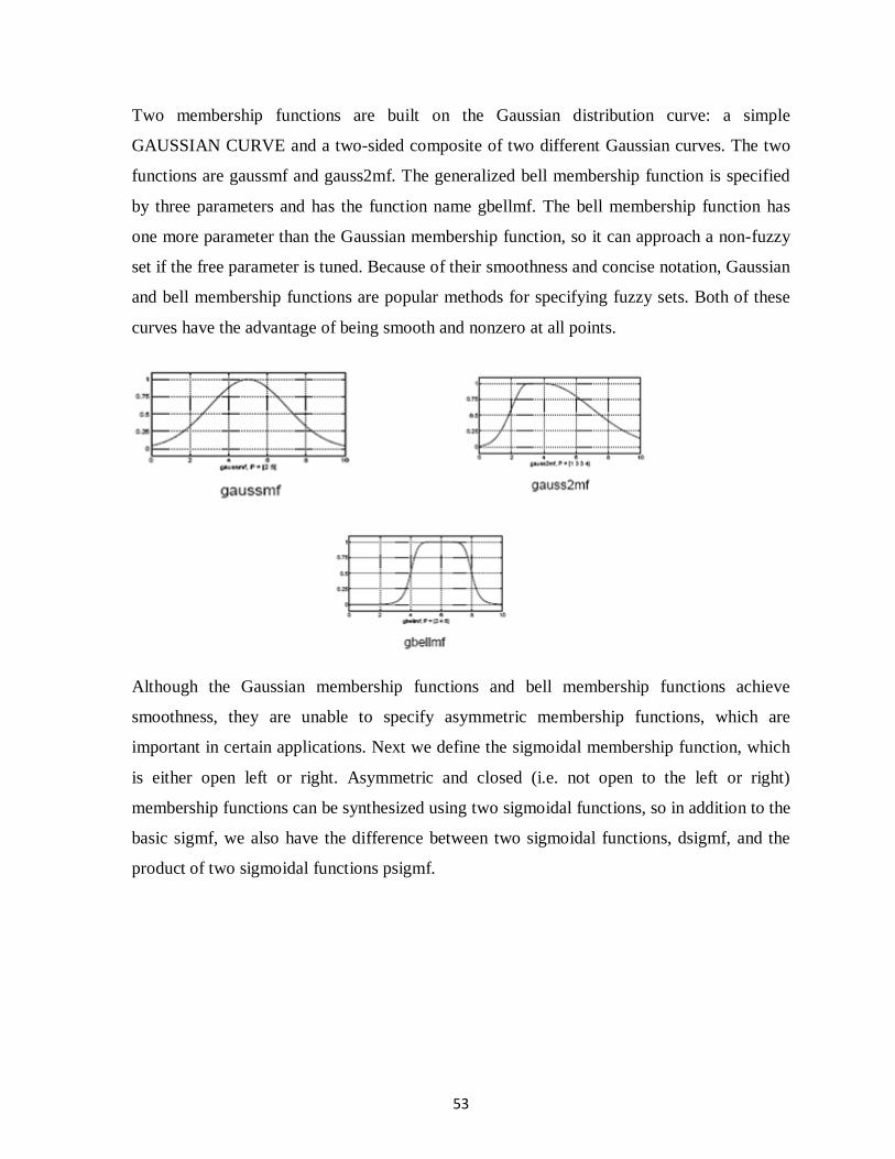
53
Two membership functions are built on the Gaussian distribution curve: a simple
GAUSSIAN CURVE and a two-sided composite of two different Gaussian curves. The two
functions are gaussmf and gauss2mf. The generalized bell membership function is specified
by three parameters and has the function name gbellmf. The bell membership function has
one more parameter than the Gaussian membership function, so it can approach a non-fuzzy
set if the free parameter is tuned. Because of their smoothness and concise notation, Gaussian
and bell membership functions are popular methods for specifying fuzzy sets. Both of these
curves have the advantage of being smooth and nonzero at all points.
Although the Gaussian membership functions and bell membership functions achieve
smoothness, they are unable to specify asymmetric membership functions, which are
important in certain applications. Next we define the sigmoidal membership function, which
is either open left or right. Asymmetric and closed (i.e. not open to the left or right)
membership functions can be synthesized using two sigmoidal functions, so in addition to the
basic sigmf, we also have the difference between two sigmoidal functions, dsigmf, and the
product of two sigmoidal functions psigmf.
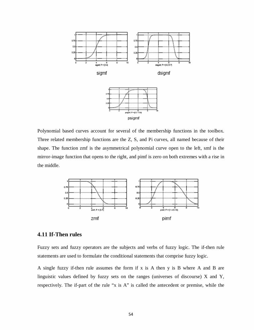
54
Polynomial based curves account for several of the membership functions in the toolbox.
Three related membership functions are the Z, S, and Pi curves, all named because of their
shape. The function zmf is the asymmetrical polynomial curve open to the left, smf is the
mirror-image function that opens to the right, and pimf is zero on both extremes with a rise in
the middle.
4.11 If-Then rules
Fuzzy sets and fuzzy operators are the subjects and verbs of fuzzy logic. The if-then rule
statements are used to formulate the conditional statements that comprise fuzzy logic.
A single fuzzy if-then rule assumes the form if x is A then y is B where A and B are
linguistic values defined by fuzzy sets on the ranges (universes of discourse) X and Y,
respectively. The if-part of the rule “x is A” is called the antecedent or premise, while the
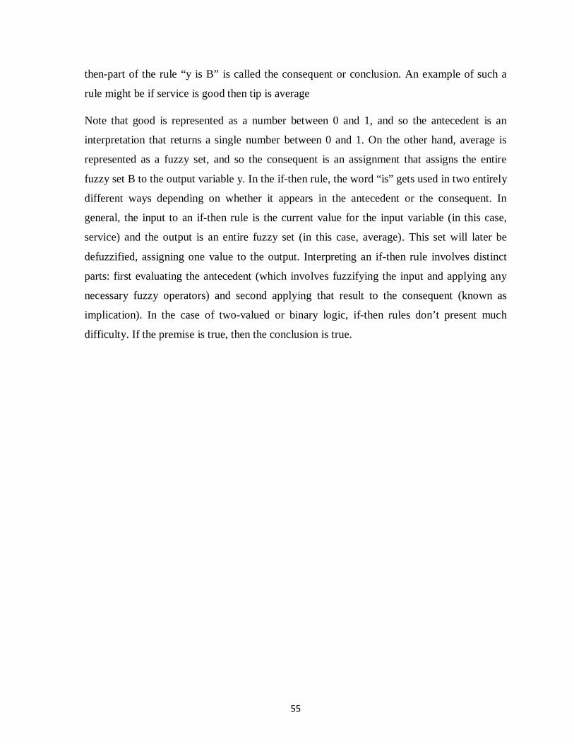
55
then-part of the rule “y is B” is called the consequent or conclusion. An example of such a
rule might be if service is good then tip is average
Note that good is represented as a number between 0 and 1, and so the antecedent is an
interpretation that returns a single number between 0 and 1. On the other hand, average is
represented as a fuzzy set, and so the consequent is an assignment that assigns the entire
fuzzy set B to the output variable y. In the if-then rule, the word “is” gets used in two entirely
different ways depending on whether it appears in the antecedent or the consequent. In
general, the input to an if-then rule is the current value for the input variable (in this case,
service) and the output is an entire fuzzy set (in this case, average). This set will later be
defuzzified, assigning one value to the output. Interpreting an if-then rule involves distinct
parts: first evaluating the antecedent (which involves fuzzifying the input and applying any
necessary fuzzy operators) and second applying that result to the consequent (known as
implication). In the case of two-valued or binary logic, if-then rules don’t present much
difficulty. If the premise is true, then the conclusion is true.
56
Chapter 5
Experimental Methodology
5.1 Fiber testing
5.1.1 AFIS
Advanced Fibre Information System is based on the single fibre testing. There are two
modules, one for testing the number of neps and the size of neps, while the other one is used
for testing the length and the diameter. Both modules can be applied separately or together.
Among all physical properties of the cotton, fiber length varies the most within any one
sample. There are two sources of variability;
1) Variability that comes from mixing cottons of various lengths
2) Variability that is biological in nature and exists within a sample of the same origin.
The same variety grown under different conditions, with lower or higher fertilizer doses,
irrigation, or pest control, can produce various lengths. This is why fibre length is tested as
an average of many fibres. Fibres also break during handling and processing thus,
emphasizing the need for measurement of magnitude of the length variation. There are many
different measurements of fibre length, including staple length, model length, mean length
(aver-age length), 2.5% span length, effective length, upper quartile length, upper-half mean
length, length uniformity index, length uniformity ratio, span length, short fibre contents and
floating fibre length.
The AFIS test provides several length parameters deduced from individual fibre
measurements. The main measurements include: the mean length, the length upper
percentiles, the length CV%, and the Short Fibre Content (defined as the percentage of fibres
less than 12.7 mm in length). Fibre length information is provided as a number or as weight-
based data (by number/by weight). The length distribution by weight is determined by the
weight-frequency of fibres in the different length categories, that is the proportion of the total
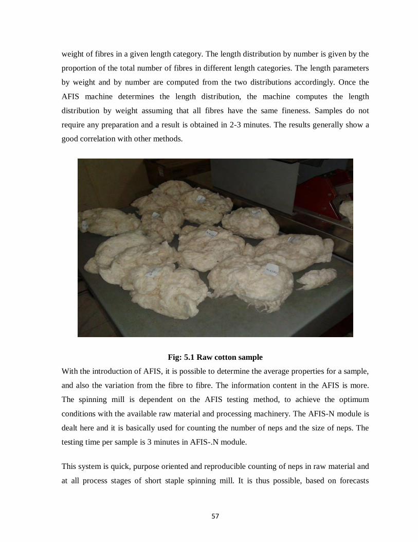
57
weight of fibres in a given length category. The length distribution by number is given by the
proportion of the total number of fibres in different length categories. The length parameters
by weight and by number are computed from the two distributions accordingly. Once the
AFIS machine determines the length distribution, the machine computes the length
distribution by weight assuming that all fibres have the same fineness. Samples do not
require any preparation and a result is obtained in 2-3 minutes. The results generally show a
good correlation with other methods.
Fig: 5.1 Raw cotton sample
With the introduction of AFIS, it is possible to determine the average properties for a sample,
and also the variation from the fibre to fibre. The information content in the AFIS is more.
The spinning mill is dependent on the AFIS testing method, to achieve the optimum
conditions with the available raw material and processing machinery. The AFIS-N module is
dealt here and it is basically used for counting the number of neps and the size of neps. The
testing time per sample is 3 minutes in AFIS-.N module.
This system is quick, purpose oriented and reproducible counting of neps in raw material and
at all process stages of short staple spinning mill. It is thus possible, based on forecasts

58
supervisory measures and early warning information to practically eliminate subsequent
complaints with respect to finished product. The lab personnel are freed from the time
consuming, delicate and unpopular, proceeding of nep counting. Personnel turnover and job
rotation no more affects the results of the nep counting. The personnel responsible for quality
can now at least deal with the unpopular neps in a more purpose-oriented manner than ever
before.
Fig: 5.2 AFIS working principle.
A fibre sample of approximately 500 mg is inserted between the feed roller and the feed plate
of the AFIS-N instrument Opening rollers open the fibre assembly and separate off the fibres,
neps, trash and dust. The trash particles and dust are suctioned off to extraction. On their way
through the transportation and acceleration channels, the fibres and neps pass through the
optical sensor, which determines the number and size of the neps. The corresponding
impulses are converted into electrical signals, which are then transmitted to a microcomputer
for evaluation purposes. According to these analyses, a distinction is made between the
single fibres and the neps. The statistical data are calculated and printed out through a printer.
The measuring process can be controlled through a PC-keyboard and a screen.

59
5.1.2 HVI (High Volume Instrument System)
The testing of fibres was always of importance to the spinner. It has been known for a long
time that the fibre characteristics have a decisive impact on the running behaviour of the
production machines, as well as on the yarn quality and manufacturing costs. In spite of the
fact that fibre characteristics are very important for yarn production, the sample size for
testing fibre characteristics is not big enough. This is due to the following
The labour and time involvement for the testing of a representative sample was too
expensive. The results were often available much too late to take corrective action.
The results often depended on the operator and / or the instrument, and could
therefore not be considered objective
One failed in trying to rationally administer the flood of the raw material data, to
evaluate such data and to introduce the necessary corrective measures.
Fig: 5.3 HVI machine
60
Only recently technical achievements have made possible the development of automatic
computer-controlled testing equipment. With their use, it is possible to quickly determine the
more important fibre characteristics.
Recent developments in HVI technology are the result of requests made by textile
manufacturers for additional and more precise fibre property information. Worldwide
competitive pressure on product price and product quality dictates close control of all
resources used in the manufacturing process.
High volume instrument systems are based on the fibre bundle testing, i.e., many fibres are
checked at the same time and their average values determined. Traditional testing using
micronaire, pressley, stelometre, and fibro graph are designed to determine average value for
a large number of fibres, the so called fibre bundle tests. In HVI, the bundle testing method is
automated.
5.2 Concepts in bale management
This is based on the categorising of cotton bales according to their fibre quality
characteristics. It includes the measurement of the fibre characteristics with reference to each
individual bale, separation of bales into classes and lying down of balanced bale mixes based
on these classes. The reason for undertaking this work lies in the fact that there is sometimes
a considerable variation in the fibre characteristics from one bale to another, even within the
same delivery. This variation will result in the yarn quality variation if the bales are mixed in
an uncontrolled manner.
The bale management software, normally embedded with an HVI, helps in selection of bales
for a particular mix from the available stock. Once the data are received from HVI in the
software, classification of bales in groups are done with user defined criteria.
· Manual calculation errors and the tedious task of day to day manual planning of mix are
avoided.
61
· The storage of large number of data enables for tracking long period records or results
thereby helping in clear analysis.
· More cost effective mix can be made since cost factor is also included. It also helps in
planning for further requirements or purchase.
· Additional details such as party name, weighment details, and rejection details can be
printed along with the test results which will be useful for the mill personnel for better
analysis.
· Separate range criteria shall be selected for basic samples, lot samples and mixing
· Flexible intervals in grouping of bales with reference to the selected category.
· Basic sample results and results checked after lot arrival shall be compared graphically or
numerically for easy decision making of approval or rejection.
The instruments are calibrated to read in staple length. Length measurements obtained from
the instrument are considerably more repeatable than the staple length determination by the
classer. In one experiment the instrument repeated the same staple length determination 44%
of the time while the classer repeated this determination only 29% of the time. Similarly, the
instrument repeated to 1/32″ on 76% of the samples, while the classer agreed on 71% of the
samples to within 1/31″.
5.2.1 Length uniformity
The HVI system gives an indication of the fibre length distribution in the bale by use of a
length uniformity index. This uniformity index is obtained by dividing the mean fibre length
by the upper-half-mean length and expressing the ratio as a percent. A reading of 80% is
considered average length uniformity. Higher numbers mean better length uniformity and
lower numbers poorer length uniformity. Cotton with a length uniformity index of 83 and
above is considered to have good length uniformity, a length uniformity index below 78 is
considered to show poor length uniformity.
62
5.2.2 Short fibre index
The measure of short-fibre content (SFC) in Motion Control’s HVI systems is based on the
fibre length distribution throughout the test specimen. It is not the staple length that is so
important but the short fibre content which is important. It is better to prefer a lower
commercial staple, but with much lower short-fibre content.
HVI systems measure length parameters of cotton samples by the fibrogram technique. The
following assumptions describe the fibro gram sampling process:
· The fibrogram sample is taken from some population of fibres.
· The probability of sampling a particular fibre is proportional to its length
· A sampled fibre will be held at a random point along its length
· A sampled fibre will project two ends away from the holding point, such that all of the ends
will be parallel and aligned at the holding point.
· All fibres have the same uniform density
The High Volume Instruments also provide empirical equations of short fibre content based
on the results of cotton produced in the United States in a particular year.
Short Fibre Index = 122.56 – (12.87 x UHM) – (1.22 x UI) -------------------(7)
where UHM – Upper Half Mean Length (inches)
UI – Uniformity Index
Short Fibre Index = 90.34 – (37.47 x SL2) – (0.90 x UR) ----------------------(8)
Where SL2 – 2.5% Span length (inches)
UR – Uniformity Ratio

63
In typical fibrogram curve, the horizontal axis represents the lengths of the ends of sampled
fibres. The vertical axis represents the percent of fibre ends in the fibrogram having that
length or greater.
5.2.3 Strength and elongation
5.2.3.1 Principle of measurement
HVI uses the “Constant rate of elongation” principle while testing the fibre sample. The
available conventional methods of strength measurement are slow and are not compatible to
be used with the HVI. The main hindering factor is the measurement of weight of the test
specimen, which is necessary to estimate the tenacity of the sample. Expression of the
breaking strength in terms of tenacity is important to make easy comparison between
specimens of varying fineness.
5.2.3.2 Method
The strength measurement made by the HVI systems is unlike the traditional laboratory
measurements of Pressley and Stelometer in several important ways. First of all the test
specimens are prepared in a very different manner. In the laboratory method the fibres are
selected, combed and carefully prepared to align them in the jaw clamps. Each and every
fibre spans the entire distance across the jaw surfaces and the space between the jaws.
Strength is measured physically by clamping a fibre bundle between 2 pairs of clamps at
known distance. The second pair of clamps pulls away from the first pair at a constant speed
until the fibre bundle breaks. The distance it travels, extending the fibre bundle before
breakage, is reported as elongation.
In the HVI instruments the fibres are randomly selected and automatically prepared for
testing. They are combed to remove loose fibres and to straighten the clamped fibres, also
brushed to remove crimp before testing. The mechanization of the specimen preparation
techniques has resulted in a “tapered” specimen where fibre ends are found in the jaw clamp
surfaces as well as in the space between the jaws.
64
A second important difference between traditional laboratory strength measurements and
HVI strength measurements is that in the laboratory measurements the mass of the broken
fibres is determined by weighing the test specimen. In the HVI systems the mass is
determined by the less direct methods of light absorption and resistance to air flow. The HVI
strength mass measurement is further complicated by having to measure the mass at the exact
point of breaks on the tapered specimen.
A third significant difference between laboratory and HVI strength measurements is the rate
or speed at which the fibres are broken. The HVI systems break the fibres about 10 times
faster than the laboratory methods.
Readings within a single bale, almost all HVI users make either 2 or 4 tests per bale and
average the readings. When the average readings are repeated within a laboratory, the
averages are repeated to within one strength unit about 80% of the time. However, when
comparisons are made between laboratories the agreement on individual bales to within plus
or minus 1 g/tex decreases to 55%.
This decrease in strength agreement between laboratories is probably related to the difficulty
of holding a constant relative humidity in the test labs. Test data indicate that 1% shift in
relative humidity will shift the strength level about 1%. For example, if the relative humidity
in the laboratory changes 3% (from 63 to 66%), the strength would change about 1 g/tex
(from 24 to 25 g/Tex)
5.2.4 Micronaire
Fibre fineness is normally expressed as a micronaire value (microgram per inch). It is
measured by relating airflow resistance to the specific surface of fibres and maturity ration is
calculated using a sophisticated algorithm based on several HVI™ measurements.
The micronaire reading given by the HVI systems is the same as has been used in the
commercial marketing of cotton for almost 25 years. The repeatability of the data and the
operator ease of performing the test have been improved slightly in the HVI micronaire

65
measurement over the original instruments by elimination of the requirement of exactly
weighing the test specimen. The micronaire instruments available today use microcomputers
to adjust the reading for a range of test specimen sizes.
The micronaire reading is considered both precise and referable. For example, if we have a
bale of cotton that has an average micronaire of 4.2 and repeatedly test samples from that
bale, over two-thirds of that micronaire readings will be between 4.1 and 4.3 and 95 %of the
readings between and 4.0 and 4.4. Thus, with only one or two tests per bale we can get a very
precise measure of the average micronaire of the bale.
The reading is influenced by both fibre maturity and fibre fineness. For a given growing area,
the cotton variety generally sets the fibre fineness, and the environmental factors control or
influence the fibre maturity. Thus, within a growing area the micronaire value is usually
highly related to the maturity value. However, on an international scale, it cannot be known
from the micronaire readings alone if cottons with different micronaire are of different
fineness or if they have different maturity levels
The measurement of cotton colour predates the measurement of micronaire, but because
colour has always been an important component of classer’s grade it has not received
attention as an independent fibre property. However the measurement of colour was
incorporated into the very early HVI systems as one of the primary fibre properties.
Determination of cotton colour requires the measurement of two properties, the grayness and
yellowness of the fibres. The grayness is a measure of the amount of light reflected from the
mass of the fibre. We call this the reflectance or Rd value. The yellowness is measured on
what we call Hunter’s +b scale after the man who developed it. The other scales that
describe colour space (blue, red, green) are not measured becasue they are considered
relatively constant for cotton.
NIR maturity and dye uptake in cotton yarns have been shown to correlate highly with
maturity as measured by NIR. A correlation of R=0.96 was obtained for a set of 15 cottons.
66
In a joint study by ITT and a European research organization, 45 cottons from four continents
were tested for maturity using the NIR method and the SHIRLEY Development Fineness/
Maturity tester (FMT). For these samples, NIR and FMT maturity correlated very highly
(R=0.94).
On 15 cottons from different growth areas of the USA, NIR maturity was found to correlate
with r2 = 0.9 through a method developed by the United States Department of Agriculture
(USDA). In this method, fibres are cross-sectioned and microscopically evaluated.
Sugar Content is a valid indicator of potential processing problems. Near infrared analysis,
because of its adaptability to HVI, allows for screening of bales prior to use. The information
serves to selected bales to avoid preparation of cotton mixes of bales with excessive sugar
content. Cotton stickiness consists of two major causes- honeydew form white flies and
aphids and high level of natural plant sugars. Both are periodic problems which cause
efficiency losses in yarn manufacturing.
5.3 Yarn strength measurement:
The data set is collected from a experiment of the tensile strength of yarn. The
UsterTensorapid 3, a standard machine for measuring tensile strength, was used to take 79
measurements of strength from each of 79 yarn cones (one of each type and 30s count, 1 lea
between measurements on each cone). The 79 measurements for each cone are not true
replications because the yarn cones should be the experimental unit. Thus we have reduced
the data by averaging over the 79 measurements for each cone.
5.3.1 Laboratory atmospheric conditions
Testing laboratories are required to maintain conditions of 70°±1° F and 65%±2% RH. All
cotton must stabilize at moisture content level of 6.75%-8.25% prior to HVI testing.

67
5.3.2 No of Sample
Size - One lea cotton yarn (1 lea =120 yards).
No. of sample – 79.
Fig: 5.4 Yarn strength measuring instrument.
5.3.3 Working procedure
1.At first one lea cotton yarn is measured by wrap reel and in this way 79 samples are taken
for testing.
2.Now, the first sample is fixed with the upper jaw and the lower jaw.
3.The m/c is started and observed the dial until the sample is torn out.
4.When the sample is torn out the m/c is stopped and the reading is taken.
5.By this way the others’ reading are taken.
6.Then all the samples are weighted and counts are calculated.
7. Tensile Strength of the all samples are calculated.
8.At last average and CV% are calculated.

68
5.4 Raw cotton data Table 5.1 Raw Cotton AFIS & HVI data
Lot No: Maturity Strength Length SFC Mic 1 0.88 32.3 29.31 7.5 4.04 2 0.9 32.7 29.82 7.8 4.44 3 0.87 28.9 28.4 8 4.21 4 0.89 28.9 28.83 9 4.65 5 0.87 29.3 29.06 8.2 4.22 6 0.88 30.5 28.55 7.8 4.31 7 0.91 33.2 29.06 9.8 4.59 8 0.87 31 28.7 8.9 4.05 9 0.88 28.6 28.65 7.8 4.49
10 0.88 31.7 29.41 8.1 4 11 0.91 34.7 29.72 8 4.52 12 0.91 33.4 29.34 6.5 4.55 13 0.88 30.2 30.81 6.2 4.39 14 0.88 32 29.31 9 4.23 15 0.9 33.4 30.2 6.5 4.41 16 0.89 31.7 29.01 8.7 4.33 17 0.89 29.4 29.72 8.6 4.59 18 0.89 33.4 31.34 8.3 4.27 19 0.91 34 30 6.8 4.67 20 0.9 33.7 29.97 7.5 4.47 21 0.89 32.1 28.55 8.4 4.35 22 0.89 31.4 30.43 8.2 4.4 23 0.9 34.8 29.08 7.1 4.31 24 0.88 31 28.32 7.3 4.3 25 0.88 30.1 28.63 7.4 4.38 26 0.89 29.2 30.71 7.7 4.56 27 0.89 32.4 29.39 8.5 4.4 28 0.9 32.3 29.62 7 4.53 29 0.89 31 30.63 4.8 4.43 30 0.9 32.4 29.03 7.7 4.47
69
Lot No: Maturity Strength Length SFC Mic 31 0.9 32 30.58 6.7 4.49 32 0.98 30.9 28.98 7.9 4.18 33 0.89 30.8 29.24 7.4 4.48 34 0.88 30.6 29.54 7.7 4.27 35 0.88 30.1 27.91 8.3 4.37 36 0.89 29.9 29.26 6.6 4.3 37 0.9 32.4 30.2 6.6 4.45 38 0.88 30.5 29.08 7.2 4.36 39 0.87 29 28.63 7.9 4.27 40 0.87 28.9 29.57 6.4 4.3 41 0.92 35.5 28.85 9.1 4.66 42 0.92 36.4 28.52 8.5 4.63 43 0.92 36.4 30.12 6.4 4.66 44 0.91 33.9 30.05 7.6 4.63 45 0.9 31.7 29.97 7.3 4.57 46 0.92 37.2 28.32 8.8 4.58 47 0.92 37.2 29.82 7.4 4.56 48 0.92 34.6 30.51 6.7 4.7 49 0.92 36.7 27.76 10.4 4.61 50 0.92 36.1 28.55 10.4 4.62 51 0.91 31.9 28.07 9 4.76 52 0.91 32.2 27.79 6.3 4.86 53 0.9 33.2 28.5 7.8 4.55 54 0.91 31.4 28.07 7.1 4.73 55 0.93 38 29.26 8.6 4.57 56 0.92 35 28.09 9 4.79 57 0.93 36 27.15 8.7 4.74 58 0.93 35.9 28.42 8.5 4.85 59 0.91 33.5 27.86 7.5 4.63 60 0.92 37.9 29.11 8.7 4.52 61 0.86 24.04 26.67 12.71 4.36 62 0.86 25.3 26.67 12.39 4.38 63 0.86 25.01 27.17 11.8 4.28 64 0.86 25.54 27.22 11.81 4.28
70
Lot No: Maturity Strength Length SFC Mic 65 0.87 25.93 27.19 11.68 4.44 66 0.86 26.18 27.21 11.18 4.31 67 0.86 26.44 27.68 11.11 4.28 68 0.87 27.27 27.56 10.51 4.37 69 0.87 27.18 27.75 10.34 4.42 70 0.86 26.7 27.73 10.7 4.18 71 0.86 27.34 27.95 10.21 4.15 72 0.84 27.77 28.19 10.55 3.72 73 0.82 27.58 28.44 10.98 3.16 74 0.87 28.62 28.51 9.5 4.25 75 0.86 28.07 28.7 9.55 4.1 76 0.86 28.56 28.85 9.45 3.98 77 0.89 29.48 29.84 8.78 4.45 78 0.87 29.57 29.96 8.68 4.16 79 0.88 31.7 30.22 8.48 4.17

71
CHAPTER 6
RESULTS AND DISCUSSION
The aims of the project was -
To predict yarn strength using fuzzy logic
To develop a fuzzy rule base relating the fibre parameters and yarn tenacity
To evaluate the modelling accuracy of fuzzy logic to predict yarn tenacity.
6.1 Selection of output parameter
The strength of a yarn is one of its most important characteristics, largely governing its
performance in further processing. Measurement of the strength of a yarn is known as tensile
testing . Tensile testing is the loading of yarn along its main axis. A weight or load is put on
the yarn that measures the load in grams, kilograms or Newton. Breaking load is the weight
at which the yarn specimen breaks. The stretch or elongation in the yarn is also measured; the
extension at break is the total increase in yarn length up to the breaking load. Extension is
measured in centimeters or millimeters given as a percentage.
If we wish to compare the results of tensile tests on yarn, the thickness and length of the yarn
specimen must be taken into account. This will give the yarn tenacity.
6.2 Selection of input parameters
The final product of yarn formation is yarn. The yarn characteristic is dependent on many
factors like spinning condition, raw material, etc. If all other condition remains constant then
raw material become major role. The influencing factors in spinning are as follows
1. Fibre strength
2. Fibre fineness
3. Short fibre percentage
4. Fibre cleanness
5. Fibre length
72
6. Fibre elongation
7. Presence of neps
8. Fibre maturity
6.3 Reason behind the selection of limited number of input parameters
Although there are eight input parameters influencing the ultimate or final product of yarn
formation process.
Fig:6.1a Matlab screen shot of fuzzy rule viewer
Let, X be the number of input parameters and Y be the number of membership functions.
Now X per the requirement, the number of rules will be vast in number with the eight inputs ,
it will create undue complicacy in our experiment. So, we have decreased the number of
inputs to four. The chosen input parameters are as follows
Fibre strength
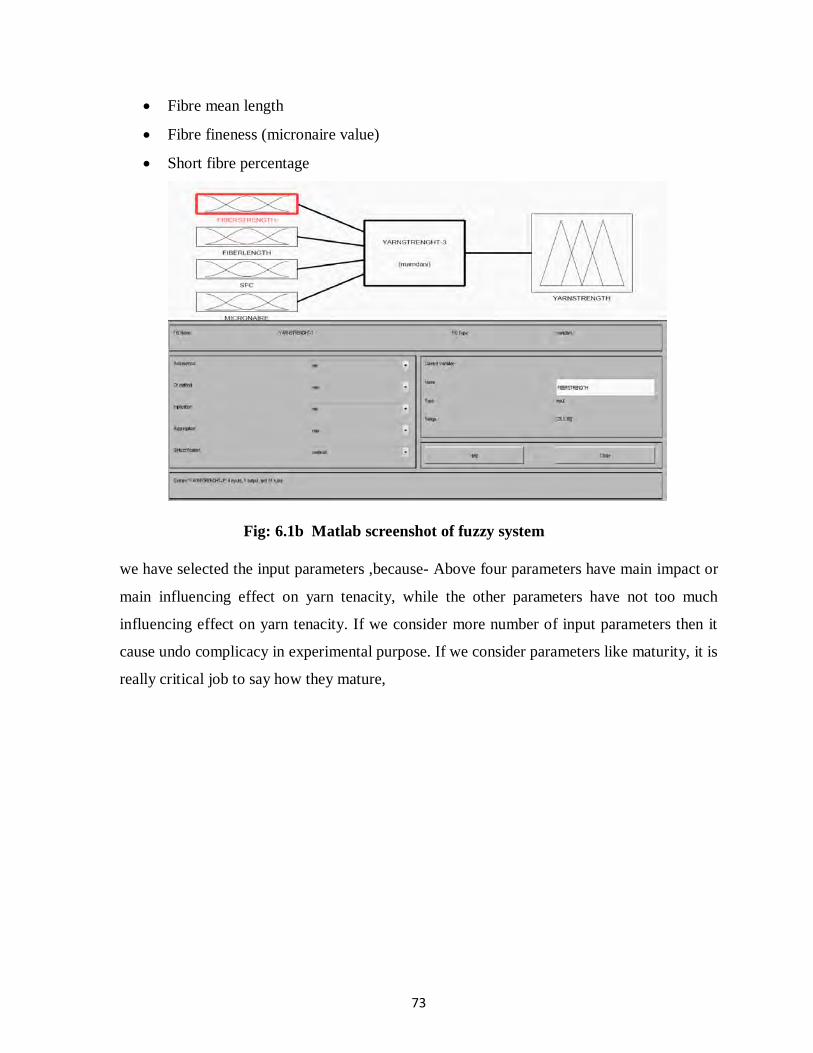
73
Fibre mean length
Fibre fineness (micronaire value)
Short fibre percentage
Fig: 6.1b Matlab screenshot of fuzzy system
we have selected the input parameters ,because- Above four parameters have main impact or
main influencing effect on yarn tenacity, while the other parameters have not too much
influencing effect on yarn tenacity. If we consider more number of input parameters then it
cause undo complicacy in experimental purpose. If we consider parameters like maturity, it is
really critical job to say how they mature,

74
Fig: 6.1c Matlab screenshot of surface view
6.4 Selection of defuzzification method
In many situations for a system in which we get the output is fuzzy, it is easier to take a crisp
decision if the output is represented as a single scalar quantity. This conversion of a fuzzy set
to single crisp value is called defuzzificition. Several methods are available in the literature
of which we illustrate a few of the widely used methods, namely centroid method, centre of
sums, and mean of maxima methods.
6.5 Cause to select certain number of membership
6.5.1 Function of input and output parameters
The membership functions need the data to be précised and should be categorized according
to the membership functions to implement them in our experiment .In case of input
parameters we have categorized three type of membership function viz. low (L),medium (M),
and high(H) by studying the range (the lower value and higher value) of the input parameters.
In case of output parameters we have taken nine type of membership function for better
prediction or result. These membership functions are:

75
Extremely low : Level 1
Very low : Level 2
Low : Level 3
Medium : Level 4
Moderately high : Level 5
Higher medium: Level 6
High : Level 7
Very high : Level 8
Extremely high : Level 9
6.6 Establishment of rules
Above all the steps, this is the most important one, because result cannot be obtained without
a bridge between input and output parameters, and rules have filled up the requirement for
us. So, there will be 81 rules for 4 input and 3 type of category of each input.(34 =81). Detail
of the fuzzy rules are given in below table
Table 6.1 Fuzzy rule
Fuzzy IF AND AND AND THEN
Rules Strength Length Mic SFC Strength Level
1 H H H H 6
2 H H H M 6
3 H H H L 6
4 H H M H 6
5 H H M M 7
6 H H M L 7
7 H H L H 6
8 H H L M 8
9 H H L L 9
10 H M H H 5

76
Fuzzy IF AND AND AND THEN
Rules Strength Length Mic SFC Strength Level
11 H M H M 5
12 H M H L 7
13 H M M H 5
14 H M M M 7
15 H M M L 8
16 H M L H 6
17 H M L M 8
18 H M L L 7
19 H L H H 5
20 H L H M 6
21 H L H L 6
22 H L M H 5
23 H L M M 5
24 H L M L 6
25 H L L H 6
26 H L L M 6
27 H L L L 4
28 M H H H 5
29 M H H M 5
30 M H H L 5
31 M H M H 5
32 M H M M 7
33 M H M L 7
34 M H L H 5
35 M H L M 7
36 M H L L 6
37 M M H H 5
38 M M H M 5
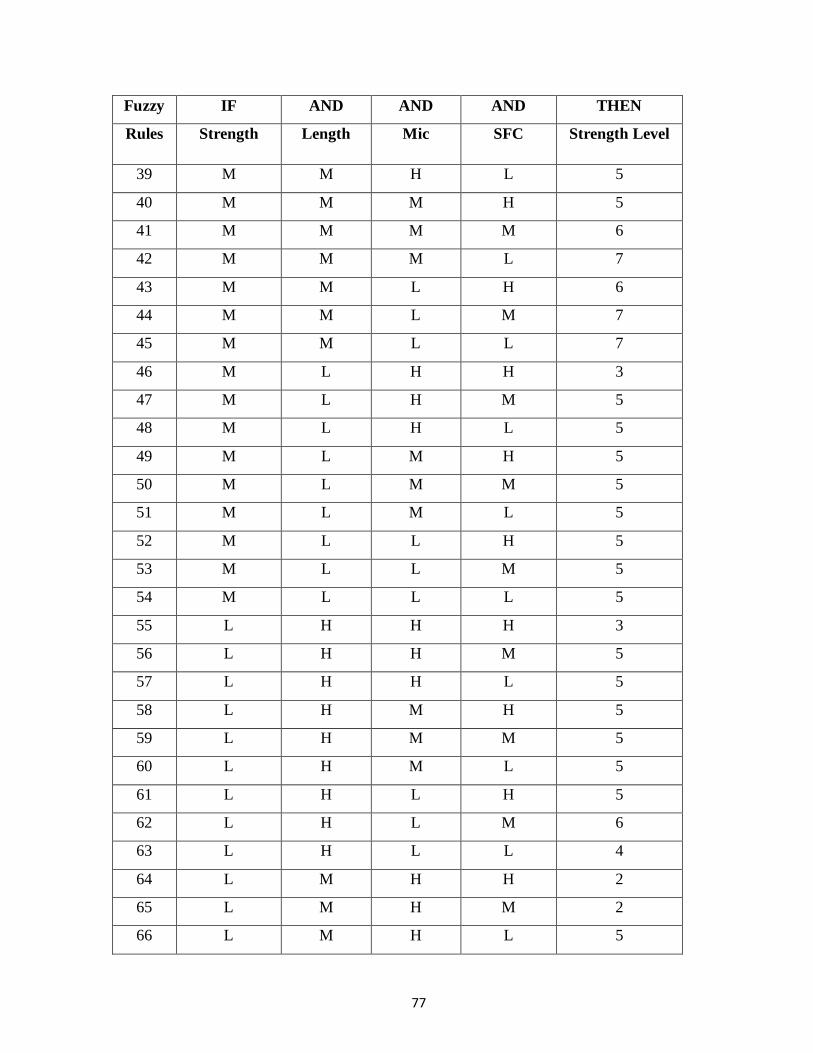
77
Fuzzy IF AND AND AND THEN
Rules Strength Length Mic SFC Strength Level
39 M M H L 5
40 M M M H 5
41 M M M M 6
42 M M M L 7
43 M M L H 6
44 M M L M 7
45 M M L L 7
46 M L H H 3
47 M L H M 5
48 M L H L 5
49 M L M H 5
50 M L M M 5
51 M L M L 5
52 M L L H 5
53 M L L M 5
54 M L L L 5
55 L H H H 3
56 L H H M 5
57 L H H L 5
58 L H M H 5
59 L H M M 5
60 L H M L 5
61 L H L H 5
62 L H L M 6
63 L H L L 4
64 L M H H 2
65 L M H M 2
66 L M H L 5

78
Fuzzy IF AND AND AND THEN
Rules Strength Length Mic SFC Strength Level
67 L M M H 2
68 L M M M 4
69 L M M L 5
70 L M L H 5
71 L M L M 5
72 L M L L 5
73 L L H H 1
74 L L H M 2
75 L L H L 4
76 L L M H 3
77 L L M M 2
78 L L M L 3
79 L L L H 4
80 L L L M 5
81 L L L L 5
6.7 Categorization of input and output parameters
The membership functions need the data to be précised and should be categorized according
to the membership functions to implement them in our experiment. Due to this reason we
have divided the input parameters (i.e. Fibre strength, Fibre mean length, Mic and SFC) into
three sections viz. low, medium & high.
Table 6.2 Input Parameters Range
Category Strength Length Mic SFC
Low 26.55 to 29.4 23.7 to 25.32 3.1 to 3.54 4.18 to 5.84
Medium 29.41 to 35.13 25.33 to 27.92 3.55 to 4.432 5.85 to 9.14
High 35.14 to 38.0 27.93 to 31.34 4.44 to 4.88 9.15 to 10.78
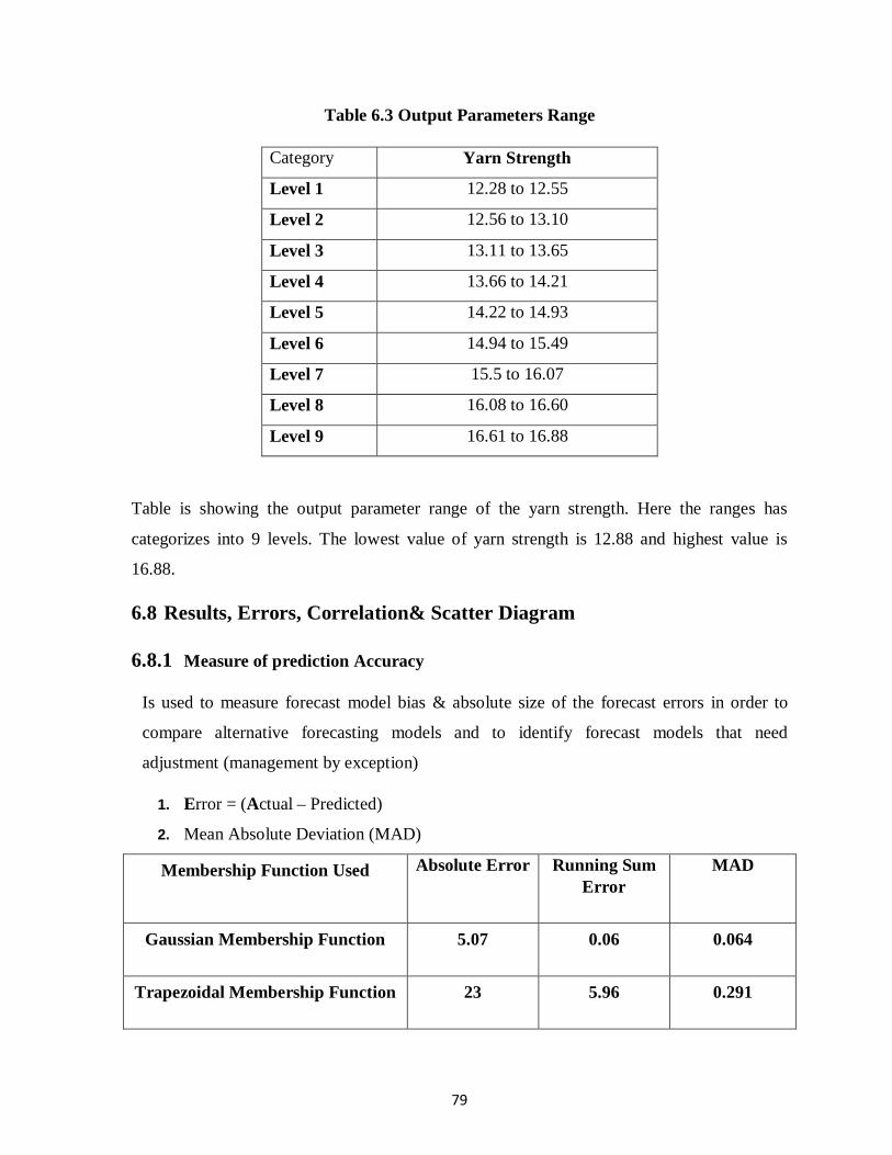
79
Table 6.3 Output Parameters Range
Category Yarn Strength
Level 1 12.28 to 12.55
Level 2 12.56 to 13.10
Level 3 13.11 to 13.65
Level 4 13.66 to 14.21
Level 5 14.22 to 14.93
Level 6 14.94 to 15.49
Level 7 15.5 to 16.07
Level 8 16.08 to 16.60
Level 9 16.61 to 16.88
Table is showing the output parameter range of the yarn strength. Here the ranges has
categorizes into 9 levels. The lowest value of yarn strength is 12.88 and highest value is
16.88.
6.8 Results, Errors, Correlation& Scatter Diagram
6.8.1 Measure of prediction Accuracy
Is used to measure forecast model bias & absolute size of the forecast errors in order to
compare alternative forecasting models and to identify forecast models that need
adjustment (management by exception)
1. Error = (Actual – Predicted)
2. Mean Absolute Deviation (MAD)
Membership Function Used Absolute Error Running Sum Error
MAD
Gaussian Membership Function 5.07 0.06 0.064
Trapezoidal Membership Function 23 5.96 0.291
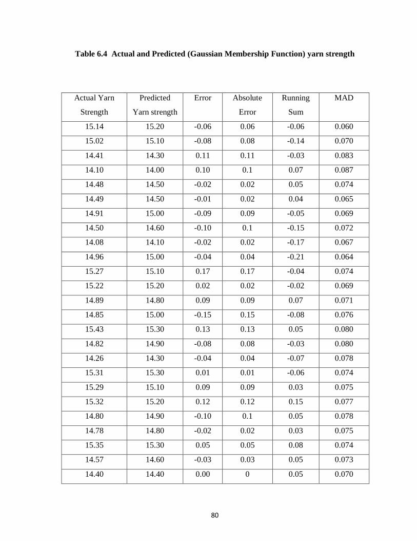
80
Table 6.4 Actual and Predicted (Gaussian Membership Function) yarn strength
Actual Yarn
Strength
Predicted
Yarn strength
Error Absolute
Error
Running
Sum
MAD
15.14 15.20 -0.06 0.06 -0.06 0.060
15.02 15.10 -0.08 0.08 -0.14 0.070
14.41 14.30 0.11 0.11 -0.03 0.083
14.10 14.00 0.10 0.1 0.07 0.087
14.48 14.50 -0.02 0.02 0.05 0.074
14.49 14.50 -0.01 0.02 0.04 0.065
14.91 15.00 -0.09 0.09 -0.05 0.069
14.50 14.60 -0.10 0.1 -0.15 0.072
14.08 14.10 -0.02 0.02 -0.17 0.067
14.96 15.00 -0.04 0.04 -0.21 0.064
15.27 15.10 0.17 0.17 -0.04 0.074
15.22 15.20 0.02 0.02 -0.02 0.069
14.89 14.80 0.09 0.09 0.07 0.071
14.85 15.00 -0.15 0.15 -0.08 0.076
15.43 15.30 0.13 0.13 0.05 0.080
14.82 14.90 -0.08 0.08 -0.03 0.080
14.26 14.30 -0.04 0.04 -0.07 0.078
15.31 15.30 0.01 0.01 -0.06 0.074
15.29 15.10 0.09 0.09 0.03 0.075
15.32 15.20 0.12 0.12 0.15 0.077
14.80 14.90 -0.10 0.1 0.05 0.078
14.78 14.80 -0.02 0.02 0.03 0.075
15.35 15.30 0.05 0.05 0.08 0.074
14.57 14.60 -0.03 0.03 0.05 0.073
14.40 14.40 0.00 0 0.05 0.070
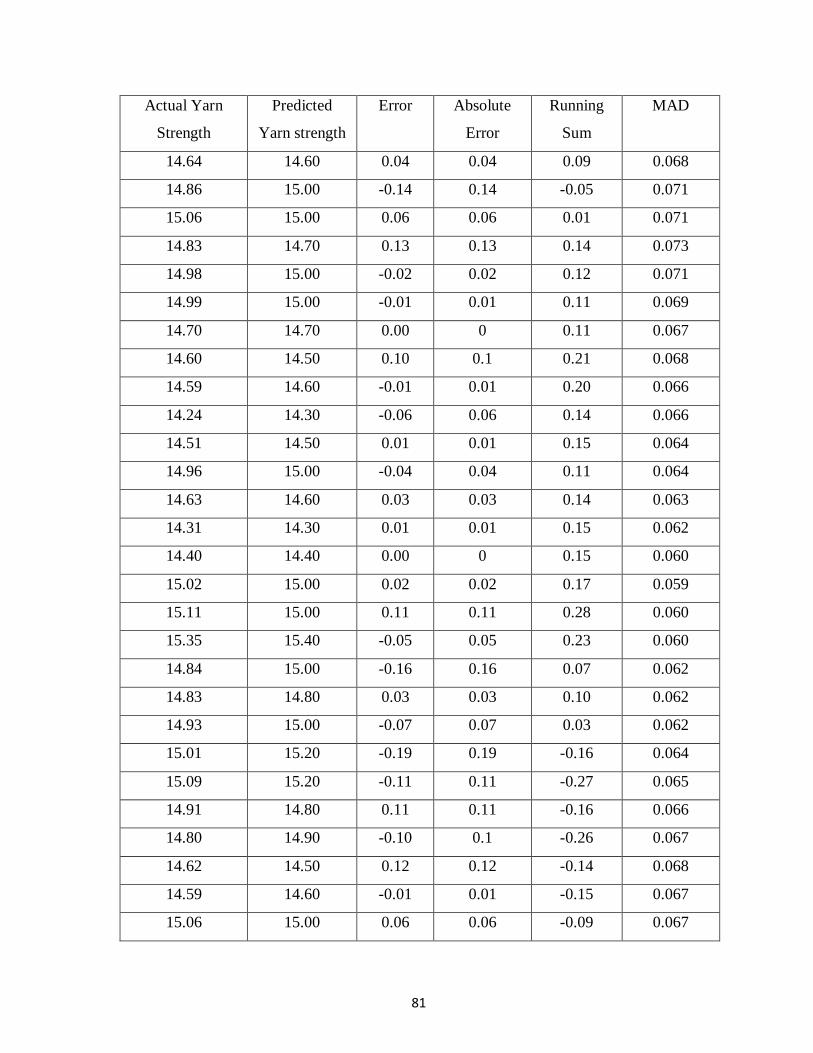
81
Actual Yarn
Strength
Predicted
Yarn strength
Error Absolute
Error
Running
Sum
MAD
14.64 14.60 0.04 0.04 0.09 0.068
14.86 15.00 -0.14 0.14 -0.05 0.071
15.06 15.00 0.06 0.06 0.01 0.071
14.83 14.70 0.13 0.13 0.14 0.073
14.98 15.00 -0.02 0.02 0.12 0.071
14.99 15.00 -0.01 0.01 0.11 0.069
14.70 14.70 0.00 0 0.11 0.067
14.60 14.50 0.10 0.1 0.21 0.068
14.59 14.60 -0.01 0.01 0.20 0.066
14.24 14.30 -0.06 0.06 0.14 0.066
14.51 14.50 0.01 0.01 0.15 0.064
14.96 15.00 -0.04 0.04 0.11 0.064
14.63 14.60 0.03 0.03 0.14 0.063
14.31 14.30 0.01 0.01 0.15 0.062
14.40 14.40 0.00 0 0.15 0.060
15.02 15.00 0.02 0.02 0.17 0.059
15.11 15.00 0.11 0.11 0.28 0.060
15.35 15.40 -0.05 0.05 0.23 0.060
14.84 15.00 -0.16 0.16 0.07 0.062
14.83 14.80 0.03 0.03 0.10 0.062
14.93 15.00 -0.07 0.07 0.03 0.062
15.01 15.20 -0.19 0.19 -0.16 0.064
15.09 15.20 -0.11 0.11 -0.27 0.065
14.91 14.80 0.11 0.11 -0.16 0.066
14.80 14.90 -0.10 0.1 -0.26 0.067
14.62 14.50 0.12 0.12 -0.14 0.068
14.59 14.60 -0.01 0.01 -0.15 0.067
15.06 15.00 0.06 0.06 -0.09 0.067

82
Actual Yarn
Strength
Predicted
Yarn strength
Error Absolute
Error
Running
Sum
MAD
14.54 14.50 0.04 0.04 -0.05 0.066
15.12 15.10 0.02 0.02 -0.03 0.065
14.95 14.80 0.15 0.15 0.12 0.067
14.64 14.70 -0.06 0.06 0.06 0.067
14.90 14.80 0.10 0.1 0.16 0.067
14.84 14.90 -0.06 0.06 0.10 0.067
14.88 15.10 -0.22 0.22 -0.12 0.070
13.36 13.40 -0.04 0.04 -0.16 0.069
13.47 13.50 -0.03 0.03 -0.19 0.069
13.57 13.50 0.07 0.07 -0.12 0.069
13.52 13.50 0.02 0.02 -0.10 0.068
13.56 13.60 -0.04 0.04 -0.14 0.068
13.76 13.70 0.06 0.06 -0.08 0.067
13.74 13.70 0.04 0.04 -0.04 0.067
13.83 13.90 -0.07 0.07 -0.11 0.067
13.77 13.80 -0.03 0.03 -0.14 0.067
13.91 13.80 0.11 0.11 -0.03 0.067
13.96 13.90 0.06 0.06 0.03 0.067
14.12 14.10 0.02 0.02 0.05 0.066
14.64 14.60 0.04 0.04 0.09 0.066
14.25 14.30 -0.05 0.05 0.04 0.066
14.34 14.40 -0.06 0.06 -0.02 0.066
14.56 14.50 0.06 0.06 0.04 0.066
14.35 14.40 -0.05 0.01 -0.01 0.065
14.71 14.70 0.01 0.01 0.00 0.064
15.16 15.10 0.06 0.06 0.06 0.064
0.06 5.07
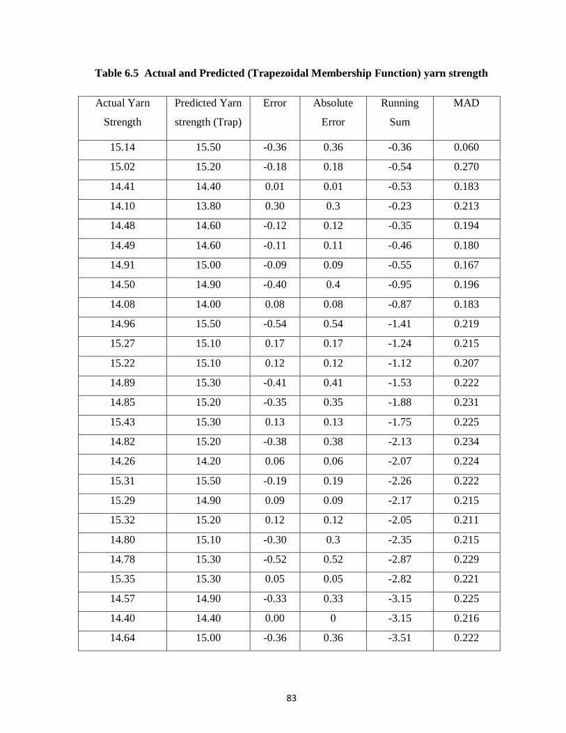
83
Table 6.5 Actual and Predicted (Trapezoidal Membership Function) yarn strength
Actual Yarn
Strength
Predicted Yarn
strength (Trap)
Error Absolute
Error
Running
Sum
MAD
15.14 15.50 -0.36 0.36 -0.36 0.060
15.02 15.20 -0.18 0.18 -0.54 0.270
14.41 14.40 0.01 0.01 -0.53 0.183
14.10 13.80 0.30 0.3 -0.23 0.213
14.48 14.60 -0.12 0.12 -0.35 0.194
14.49 14.60 -0.11 0.11 -0.46 0.180
14.91 15.00 -0.09 0.09 -0.55 0.167
14.50 14.90 -0.40 0.4 -0.95 0.196
14.08 14.00 0.08 0.08 -0.87 0.183
14.96 15.50 -0.54 0.54 -1.41 0.219
15.27 15.10 0.17 0.17 -1.24 0.215
15.22 15.10 0.12 0.12 -1.12 0.207
14.89 15.30 -0.41 0.41 -1.53 0.222
14.85 15.20 -0.35 0.35 -1.88 0.231
15.43 15.30 0.13 0.13 -1.75 0.225
14.82 15.20 -0.38 0.38 -2.13 0.234
14.26 14.20 0.06 0.06 -2.07 0.224
15.31 15.50 -0.19 0.19 -2.26 0.222
15.29 14.90 0.09 0.09 -2.17 0.215
15.32 15.20 0.12 0.12 -2.05 0.211
14.80 15.10 -0.30 0.3 -2.35 0.215
14.78 15.30 -0.52 0.52 -2.87 0.229
15.35 15.30 0.05 0.05 -2.82 0.221
14.57 14.90 -0.33 0.33 -3.15 0.225
14.40 14.40 0.00 0 -3.15 0.216
14.64 15.00 -0.36 0.36 -3.51 0.222
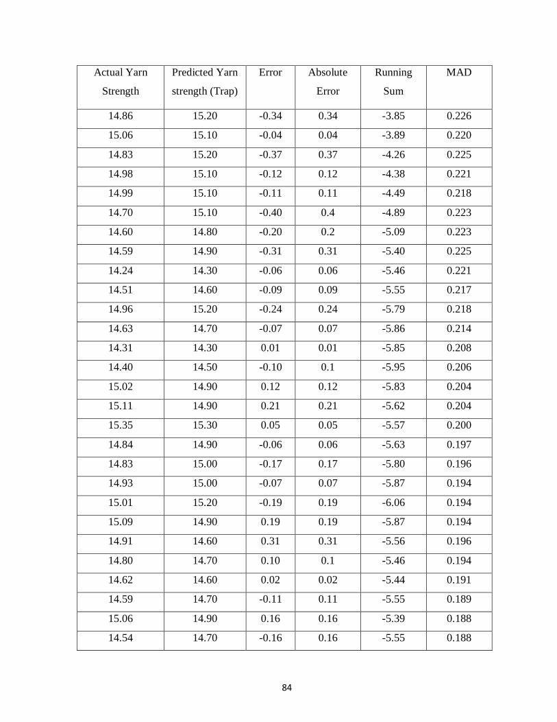
84
Actual Yarn
Strength
Predicted Yarn
strength (Trap)
Error Absolute
Error
Running
Sum
MAD
14.86 15.20 -0.34 0.34 -3.85 0.226
15.06 15.10 -0.04 0.04 -3.89 0.220
14.83 15.20 -0.37 0.37 -4.26 0.225
14.98 15.10 -0.12 0.12 -4.38 0.221
14.99 15.10 -0.11 0.11 -4.49 0.218
14.70 15.10 -0.40 0.4 -4.89 0.223
14.60 14.80 -0.20 0.2 -5.09 0.223
14.59 14.90 -0.31 0.31 -5.40 0.225
14.24 14.30 -0.06 0.06 -5.46 0.221
14.51 14.60 -0.09 0.09 -5.55 0.217
14.96 15.20 -0.24 0.24 -5.79 0.218
14.63 14.70 -0.07 0.07 -5.86 0.214
14.31 14.30 0.01 0.01 -5.85 0.208
14.40 14.50 -0.10 0.1 -5.95 0.206
15.02 14.90 0.12 0.12 -5.83 0.204
15.11 14.90 0.21 0.21 -5.62 0.204
15.35 15.30 0.05 0.05 -5.57 0.200
14.84 14.90 -0.06 0.06 -5.63 0.197
14.83 15.00 -0.17 0.17 -5.80 0.196
14.93 15.00 -0.07 0.07 -5.87 0.194
15.01 15.20 -0.19 0.19 -6.06 0.194
15.09 14.90 0.19 0.19 -5.87 0.194
14.91 14.60 0.31 0.31 -5.56 0.196
14.80 14.70 0.10 0.1 -5.46 0.194
14.62 14.60 0.02 0.02 -5.44 0.191
14.59 14.70 -0.11 0.11 -5.55 0.189
15.06 14.90 0.16 0.16 -5.39 0.188
14.54 14.70 -0.16 0.16 -5.55 0.188
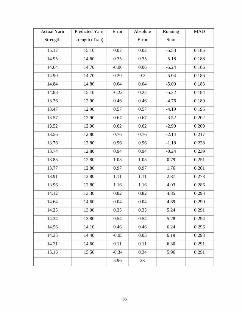
85
Actual Yarn
Strength
Predicted Yarn
strength (Trap)
Error Absolute
Error
Running
Sum
MAD
15.12 15.10 0.02 0.02 -5.53 0.185
14.95 14.60 0.35 0.35 -5.18 0.188
14.64 14.70 -0.06 0.06 -5.24 0.186
14.90 14.70 0.20 0.2 -5.04 0.186
14.84 14.80 0.04 0.04 -5.00 0.183
14.88 15.10 -0.22 0.22 -5.22 0.184
13.36 12.90 0.46 0.46 -4.76 0.189
13.47 12.90 0.57 0.57 -4.19 0.195
13.57 12.90 0.67 0.67 -3.52 0.202
13.52 12.90 0.62 0.62 -2.90 0.209
13.56 12.80 0.76 0.76 -2.14 0.217
13.76 12.80 0.96 0.96 -1.18 0.228
13.74 12.80 0.94 0.94 -0.24 0.239
13.83 12.80 1.03 1.03 0.79 0.251
13.77 12.80 0.97 0.97 1.76 0.261
13.91 12.80 1.11 1.11 2.87 0.273
13.96 12.80 1.16 1.16 4.03 0.286
14.12 13.30 0.82 0.82 4.85 0.293
14.64 14.60 0.04 0.04 4.89 0.290
14.25 13.90 0.35 0.35 5.24 0.291
14.34 13.80 0.54 0.54 5.78 0.294
14.56 14.10 0.46 0.46 6.24 0.296
14.35 14.40 -0.05 0.05 6.19 0.293
14.71 14.60 0.11 0.11 6.30 0.291
15.16 15.50 -0.34 0.34 5.96 0.291
5.96 23
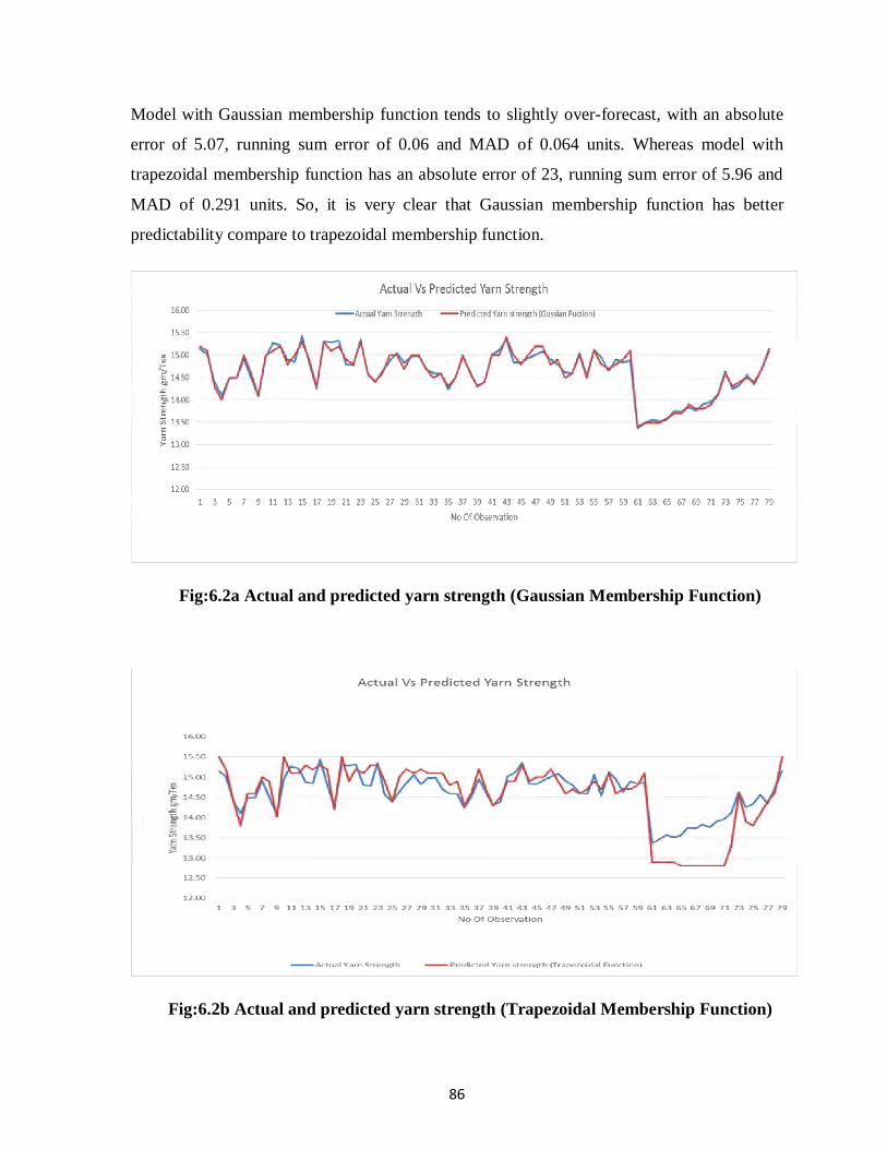
86
Model with Gaussian membership function tends to slightly over-forecast, with an absolute
error of 5.07, running sum error of 0.06 and MAD of 0.064 units. Whereas model with
trapezoidal membership function has an absolute error of 23, running sum error of 5.96 and
MAD of 0.291 units. So, it is very clear that Gaussian membership function has better
predictability compare to trapezoidal membership function.
Fig:6.2a Actual and predicted yarn strength (Gaussian Membership Function)
Fig:6.2b Actual and predicted yarn strength (Trapezoidal Membership Function)

87
6.8.2 Correlations
Pearson's correlation coefficient between two variables is defined as the covariance of the
two variables divided by the product of their standard deviations. The form of the definition
involves a "product moment", that is, the mean (the first moment about the origin) of the
product of the mean-adjusted random variables; hence the modifier product-moment in the
name.
In statistics, Cronbach's alpha (alpha) is a coefficient of internal consistency. It is commonly
used as an estimate of the reliability of a psychometric test for a sample of examinees. It was
first named alpha by Lee Cronbach in 1951, as he had intended to continue with further
coefficients. The measure can be viewed as an extension of the Kuder–Richardson Formula
20 (KR-20), which is an equivalent measure for dichotomous items. Alpha is not robust
against missing data. Several other Greek letters have been used by later researchers to
designate other measures used in a similar context. Somewhat related is the average variance
extracted (AVE). The theoretical value of alpha varies from zero to 1, since it is the ratio of
two variances. However, depending on the estimation procedure used, estimates of alpha can
take on any value less than or equal to 1, including negative values, although only positive
values make sense. Higher values of alpha are more desirable. Some professionals, as a rule
of thumb, require a reliability of 0.70 or higher (obtained on a substantial sample) before they
will use an instrument. Obviously, this rule should be applied with caution when alpha has
been computed from items that systematically violate its assumptions.[specify] Furthermore,
the appropriate degree of reliability depends upon the use of the instrument. For example, an
instrument designed to be used as part of a battery of tests may be intentionally designed to
be as short as possible, and therefore somewhat less reliable. Other situations may require
extremely precise measures with very high reliabilities. In the extreme case of a two-item
test, the Spearman–Brown prediction formula is more appropriate than Cronbach's alpha.
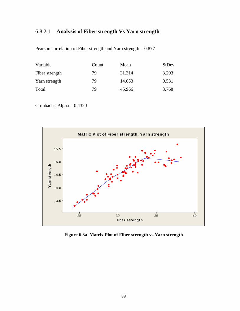
88
6.8.2.1 Analysis of Fiber strength Vs Yarn strength
Pearson correlation of Fiber strength and Yarn strength = 0.877
Variable Count Mean StDev
Fiber strength 79 31.314 3.293
Yarn strength 79 14.653 0.531
Total 79 45.966 3.768
Cronbach's Alpha = 0.4320
40353025
15.5
15.0
14.5
14.0
13.5
Fiber strength
Yar
n st
reng
th
Matrix Plot of Fiber strength, Yarn strength
Figure 6.3a Matrix Plot of Fiber strength vs Yarn strength

89
6.8.2.2 Analysis of Length Vs Yarn strength
Pearson correlation of Length and Yarn strength = 0.679
Variable Count Mean StDev
Length 79 28.923 1.039
Yarn strength 79 14.653 0.531
Total 79 43.575 1.452
Cronbach's Alpha = 0.7100
3130292827
15.5
15.0
14.5
14.0
13.5
Length
Yar
n st
reng
th
Matrix Plot of Length, Yarn strength
Figure 6.3b Matrix Plot of Length vs Yarn strength

90
6.8.2.3 Analysis of SFC, Yarn strength
Pearson correlation of SFC and Yarn strength = -0.684
Variable Count Mean StDev
SFC 79 8.481 1.597
Yarn strength 79 14.653 0.531
Total 79 23.134 1.293
Cronbach's Alpha = -1.388
1210864
15.5
15.0
14.5
14.0
13.5
SFC
Yar
n st
reng
th
Matrix Plot of SFC, Yarn strength
Figure 6.3c Matrix Plot of SFC vs Yarn strength
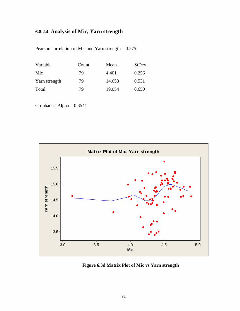
91
6.8.2.4 Analysis of Mic, Yarn strength
Pearson correlation of Mic and Yarn strength = 0.275
Variable Count Mean StDev
Mic 79 4.401 0.256
Yarn strength 79 14.653 0.531
Total 79 19.054 0.650
Cronbach's Alpha = 0.3541
5.04.54.03.53.0
15.5
15.0
14.5
14.0
13.5
Mic
Yar
n st
reng
th
Matrix Plot of Mic, Yarn strength
Figure 6.3d Matrix Plot of Mic vs Yarn strength

92
Cronbach's alpha will generally increase as the intercorrelations among test items increase,
and is thus known as an internal consistency estimate of reliability of test scores. Because
intercorrelations among test items are maximized when all items measure the same construct,
Cronbach's alpha is widely believed to indirectly indicate the degree to which a set of items
measures a single unidimensional latent construct. However, the average intercorrelation
among test items is affected by skew just like any other average. Thus, whereas the modal
intercorrelation among test items will equal zero when the set of items measures several
unrelated latent constructs, the average intercorrelation among test items will be greater than
zero in this case. Indeed, several investigators have shown that alpha can take on quite high
values even when the set of items measures several unrelated latent constructs. As a result,
alpha is most appropriately used when the items measure different substantive areas within a
single construct. When the set of items measures more than one construct, coefficient omega
hierarchical is more appropriate. Alpha treats any covariance among items as true-score
variance, even if items covary for spurious reasons. For example, alpha can be artificially
inflated by making scales which consist of superficial changes to the wording within a set of
items or by analyzing speeded tests.

93
6.8.3 Analysis of Variances:
The statistical model for which one-way ANOVA is appropriate is that the (quantitative)
outcomes for each group are normally distributed with a common variance. The errors
(deviations of individual outcomes from the population group means) are assumed to be
independent. The model places no restrictions on the population group means.
6.8.3.1 One-way ANOVA: Yarn strength versus Fiber strength
Source DF SS MS F P
Fiber strength 59 21.6414 0.3668 19.57 0.000
Error 19 0.3562 0.0187
Total 78 21.9976
S = 0.1369 R-Sq = 98.38% R-Sq(adj) = 93.35%
In this case the p value is 0 which is less than the critical value that indicates that Yarn
strength versus Fiber strength is statistically significant at 5% level of significance. The R-Sq
indicates strong linear relationship between this two variables.
6.8.3.2 One-way ANOVA: Yarn strength versus Length
Source DF SS MS F P
Length 62 20.4013 0.3291 3.30 0.005
Error 16 1.5963 0.0998
Total 78 1.9976
S = 0.3159 R-Sq = 92.74% R-Sq(adj) = 64.62%
In this case the p value is 0.005 which is less than the critical value that indicates that Yarn
strength versus Length is statistically significant at 5% level of significance. The R-Sq
indicates strong linear relationship between these two variables.
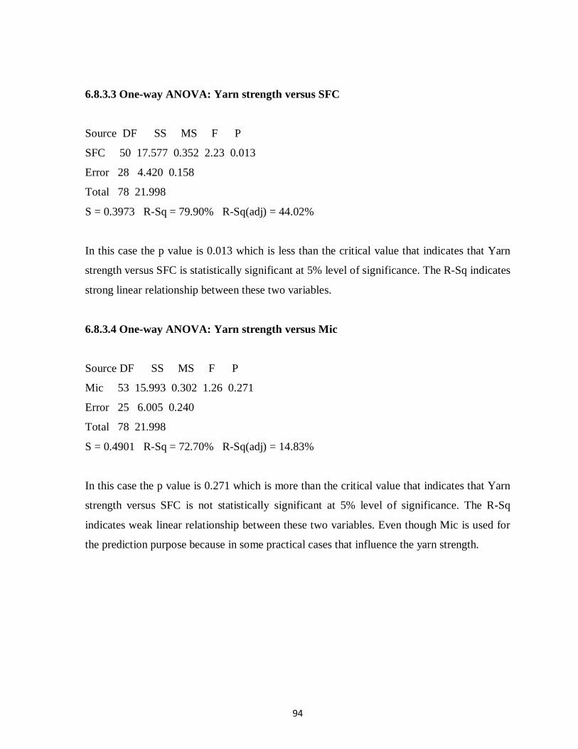
94
6.8.3.3 One-way ANOVA: Yarn strength versus SFC
Source DF SS MS F P
SFC 50 17.577 0.352 2.23 0.013
Error 28 4.420 0.158
Total 78 21.998
S = 0.3973 R-Sq = 79.90% R-Sq(adj) = 44.02%
In this case the p value is 0.013 which is less than the critical value that indicates that Yarn
strength versus SFC is statistically significant at 5% level of significance. The R-Sq indicates
strong linear relationship between these two variables.
6.8.3.4 One-way ANOVA: Yarn strength versus Mic
Source DF SS MS F P
Mic 53 15.993 0.302 1.26 0.271
Error 25 6.005 0.240
Total 78 21.998
S = 0.4901 R-Sq = 72.70% R-Sq(adj) = 14.83%
In this case the p value is 0.271 which is more than the critical value that indicates that Yarn
strength versus SFC is not statistically significant at 5% level of significance. The R-Sq
indicates weak linear relationship between these two variables. Even though Mic is used for
the prediction purpose because in some practical cases that influence the yarn strength.

95
CHAPTER 7
CONCLUSIONS
A fuzzy expert system has been developed to predict the yarn strength. The expert system
was developed by translating the perception and experience of a spinner into fuzzy inference
system. The developed fuzzy rules give a very good understanding about the interaction
between important fibre parameters and their influence on yarn tenacity. The prediction
accuracy of the proposed fuzzy system is reasonably good as the mean error% of prediction
was below 5% for Gaussian membership functions. The system is quite easy to develop and
it could be modified easily if the spinning technology is changed.
Further attempts could be made to incorporate more input variables in the expert system so
that the modelling accuracy could be enhanced. But that would require large number of
computing and highly configured computer. In addition neural network also can be
incorporated with fuzzy system which is called ANFIS to get more precise result. Finally, the
work is done for one variety of raw cotton (CIS Uzbekistan), but in real world a large variety
of cotton are used in spinning mills. So there is a scope to do the project work in large scale
including all varieties of raw cotton with different origin like USA, Egypt, China, India etc.

96
REFERENCES
1. Y. E. El Mogahzy, “Selecting cotton fiber properties for fitting reliable equations to HVI data,” Textile Research Journal, vol. 58, no. 7, pp. 392–397, 1988.
2. S. Ertugrul and N. Ucar, “Predicting bursting strength of cotton plain knitted fabrics using intelligent techniques,” Textile Research Journal, vol. 70, no. 10, pp. 845–851, 2000.
3. M. D. Ethridge, J. D. Towery, and J. F. Hembree, “Estimating functional relationships between fiber properties and the strength of open-end spun yarns,” Textile Research Journal, vol. 52, no. 1, pp. 35–45, 1982.
4. C. Price, H. Senter, J. Foulk, G. Gamble, and W. Meredith, “Relationship of fiber properties to vortex yarn quality via partial least squares,” Journal of Engineered Fibers and Fabrics, vol. 4, no. 4, pp. 37–46, 2009.
5. M. E. ¨ Ureyen and H. Kadoˇglu, “Regressional estimation of ring cotton yarn properties from HVI fiber properties,” Textile Research Journal, vol. 76, no. 5, pp. 360–366, 2006.
6. M. W. Suh, K. Hyun-Jui, and C. Xiaoling, “Prediction of yarn tensile properties based on HVI testing of 36 U.S. Upland cottons,” in Proceedings of the Beltwide Cotton Conferences, pp. 786–790, San Diego, Calif, USA, January 1998.
7. M. C. Ramesh, R. Rajamanickam, and S. Jayaraman, “Prediction of yarn tensile properties by using artificial neural networks,” Journal of the Textile Institute, vol. 86, no. 3, pp. 459–469, 1995.
8. R. Zhu and M. D. Ethridge, “The prediction of cotton yarn irregularity based on the ‘AFIS’ measurement,” Journal of Textile Institute, vol. 87, no. 3, pp. 509–512, 1996.
9. A. Guha, R. Chattopadhyay, and B. Jayadeva, “Predicting yarn tenacity: a comparison of mechanistic, statistical, and neural network models,” Journal of the Textile Institute , vol. 92, no. 1, pp. 139–145, 2001.
10. A.Majumdar, A. Ghosh, S. S. Saha et al., “Empirical modelling of tensile strength of woven fabrics,” Fibers and Polymers, vol. no. 2, pp. 240–245, 2008.
11. M. Zeydan, “Modelling the woven fabric strength using artificial neural network and Taguchimethodologies,” International Journal of Clothing Science and Technology, vol. 20, no. 2, pp. 104–118, 2008.
12. J.-G. Yang, Z.-J. Lv, and Q. Xiang, “Yarn properties prediction using support vector machines: an intelligent reasoning method,” in Proceedings of the 4th International Conference on Fuzzy Systems and Knowledge Discovery (FSKD ’07), vol. 1, pp. 696–700, Haikou, China, August 2007.
13. Z. Bo, “Predicting fiber diameter of Polypropylene (PP) spunbonding nonwovens process: a comparison between physical and artifical neural network methods,” in
97
Proceedings of the International Conference on Computational Intelligence and Security (CIS ’09), vol. 1, pp. 639–642, Beijing, China, December 2009.
14. B. Chylewska and D. Cyniak, “Requirements for fibres used for rotor-spun yarns,” Bulletin of the Gdynia Cotton Association, no. 4, pp. 33–47, 1998 (Polish).
15. T. Jackowski and I. Frydrych, “What i learnt in fibre quality: practical experience,” in Proceedings of the 58th Plenary Meeting of the International Cotton Advisory Committee, Charleston, SC, USA, October 1999.
16. M. Frey, “Influence of fibre parameters and values of their variation on the spinning process,” in Proceedings of the 4th International Conference on Grid Computing and Applications, Gdynia, Poland, 1995.
17. M. Kilic¸ and A. Okur, “Relationships between yarn diameter/ diameter variation and strength,” Fibres and Textiles in Eastern Europe, vol. 14, no. 5, pp. 84–87, 2006.
18. Fuzzy Sets, LA Zadeh- Information and control,1965.

98
Matlab Code:
Name='YARNSTRENGHT-3'
Type='mamdani'
Version=2.0
NumInputs=4
NumOutputs=1
NumRules=81
AndMethod='min'
OrMethod='max'
ImpMethod='min'
AggMethod='max'
DefuzzMethod='centroid'
[Input1]
Name='FIBERSTRENGTH'
Range=[26.5 38]
NumMFs=3
MF1='LOW':'gaussmf',[2.441 26.55]
MF2='MEDIUM':'gaussmf',[2.441 32.25]
MF3='HIGH':'gaussmf',[2.441 38]
[Input2]
Name='FIBERLENGTH'
Range=[23.7 31.34]
NumMFs=3
MF1='LOW':'gaussmf',[1.622 23.7]
MF2='MEDIUM':'gaussmf',[1.622 27.52]
MF3='HIGH':'gaussmf',[1.622 31.34]
[Input3]
Name='SFC'

99
Range=[4.2 10.8]
NumMFs=3
MF1='LOW':'gaussmf',[1.401 4.182]
MF2='MEDIUM':'gaussmf',[1.401 7.5]
MF3='HIGH':'gaussmf',[1.401 10.78]
[Input4]
Name='MICRONAIRE'
Range=[3.1 4.88]
NumMFs=3
MF1='LOW':'gaussmf',[0.3779 3.1]
MF2='MEDIUM':'gaussmf',[0.3779 3.985]
MF3='HIGH':'gaussmf',[0.3779 4.88]
[Output1]
Name='YARNSTRENGTH'
Range=[12.28 16.88]
NumMFs=9
MF1='LEVEL_1':'gaussmf',[0.2442 12.28]
MF2='LEVEL_2':'gaussmf',[0.2442 12.83]
MF3='LEVEL_3':'gaussmf',[0.2442 13.38]
MF4='LEVEL_4':'gaussmf',[0.2442 13.96]
MF5='LEVEL_5':'gaussmf',[0.2442 14.65]
MF6='LEVEL_6':'gaussmf',[0.2442 15.2]
MF7='LEVEL_7':'gaussmf',[0.2442 15.78]
MF8='LEVEL_8':'gaussmf',[0.2442 16.33]
MF9='LEVEL_9':'gaussmf',[0.2442 16.88]
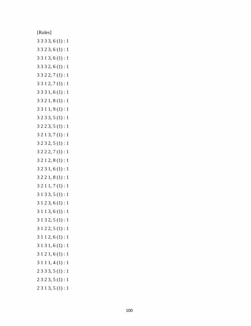
100
[Rules]
3 3 3 3, 6 (1) : 1
3 3 2 3, 6 (1) : 1
3 3 1 3, 6 (1) : 1
3 3 3 2, 6 (1) : 1
3 3 2 2, 7 (1) : 1
3 3 1 2, 7 (1) : 1
3 3 3 1, 6 (1) : 1
3 3 2 1, 8 (1) : 1
3 3 1 1, 9 (1) : 1
3 2 3 3, 5 (1) : 1
3 2 2 3, 5 (1) : 1
3 2 1 3, 7 (1) : 1
3 2 3 2, 5 (1) : 1
3 2 2 2, 7 (1) : 1
3 2 1 2, 8 (1) : 1
3 2 3 1, 6 (1) : 1
3 2 2 1, 8 (1) : 1
3 2 1 1, 7 (1) : 1
3 1 3 3, 5 (1) : 1
3 1 2 3, 6 (1) : 1
3 1 1 3, 6 (1) : 1
3 1 3 2, 5 (1) : 1
3 1 2 2, 5 (1) : 1
3 1 1 2, 6 (1) : 1
3 1 3 1, 6 (1) : 1
3 1 2 1, 6 (1) : 1
3 1 1 1, 4 (1) : 1
2 3 3 3, 5 (1) : 1
2 3 2 3, 5 (1) : 1
2 3 1 3, 5 (1) : 1
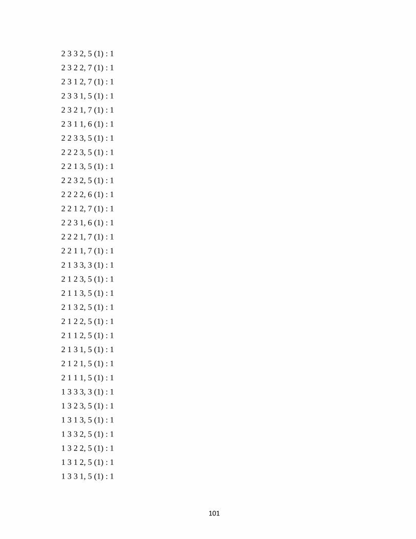
101
2 3 3 2, 5 (1) : 1
2 3 2 2, 7 (1) : 1
2 3 1 2, 7 (1) : 1
2 3 3 1, 5 (1) : 1
2 3 2 1, 7 (1) : 1
2 3 1 1, 6 (1) : 1
2 2 3 3, 5 (1) : 1
2 2 2 3, 5 (1) : 1
2 2 1 3, 5 (1) : 1
2 2 3 2, 5 (1) : 1
2 2 2 2, 6 (1) : 1
2 2 1 2, 7 (1) : 1
2 2 3 1, 6 (1) : 1
2 2 2 1, 7 (1) : 1
2 2 1 1, 7 (1) : 1
2 1 3 3, 3 (1) : 1
2 1 2 3, 5 (1) : 1
2 1 1 3, 5 (1) : 1
2 1 3 2, 5 (1) : 1
2 1 2 2, 5 (1) : 1
2 1 1 2, 5 (1) : 1
2 1 3 1, 5 (1) : 1
2 1 2 1, 5 (1) : 1
2 1 1 1, 5 (1) : 1
1 3 3 3, 3 (1) : 1
1 3 2 3, 5 (1) : 1
1 3 1 3, 5 (1) : 1
1 3 3 2, 5 (1) : 1
1 3 2 2, 5 (1) : 1
1 3 1 2, 5 (1) : 1
1 3 3 1, 5 (1) : 1

102
1 3 2 1, 5 (1) : 1
1 3 1 1, 4 (1) : 1
1 2 3 3, 2 (1) : 1
1 2 2 3, 2 (1) : 1
1 2 1 3, 5 (1) : 1
1 2 3 2, 2 (1) : 1
1 2 2 2, 4 (1) : 1
1 2 1 2, 5 (1) : 1
1 2 3 1, 5 (1) : 1
1 2 2 1, 5 (1) : 1
1 2 1 1, 5 (1) : 1
1 1 3 3, 1 (1) : 1
1 1 2 3, 2 (1) : 1
1 1 1 3, 4 (1) : 1
1 1 3 2, 3 (1) : 1
1 1 2 2, 2 (1) : 1
1 1 1 2, 3 (1) : 1
1 1 3 1, 4 (1) : 1
1 1 2 1, 5 (1) : 1
1 1 1 1, 5 (1) : 1