Prediction of the Maximum Dislocation Density in Lath Martensitic Steelby Elasto-Plastic Phase-Field Method

Zhenhua Cong1, Yoshinori Murata1,+, Yuhki Tsukada2 and Toshiyuki Koyama2

1Department of Materials, Physics and Energy Engineering, Graduate School of Engineering,Nagoya University, Nagoya 464-8603, Japan2Department of Materials Science and Engineering, Graduate School of Engineering,Nagoya Institute of Technology, Nagoya 466-8555, Japan

On the basis of the two types of slip deformation (TTSD) model of lath martensite, the martensitic transformation was simulated in Fe­0.1mass% C steel by an elasto-plastic phase-field method. The TTSD model allowed us to predict the total dislocations for the necessity of theformation of lath martensite, which is taken as the upper limit of dislocation density in lath martensite. The calculated dislocation density by thesimulation was reasonable to be higher than the observed dislocations in value but to be the same in order. This consistence indicates that thecalculation method based on the TTSD model is credible, together with the calculation of the habit plane predicted by the TTSD model.[doi:10.2320/matertrans.M2012067]

(Received February 20, 2012; Accepted June 25, 2012; Published August 8, 2012)

Keywords: dislocation density, slip deformation, phase-field method, lath martensite

1. Introduction

The martensite phase in steels exhibits several morphol-ogies such as lath, plate and butterfly, depending on thealloying elements.1,2) Among them, lath martensite exhibitshigh strength, wear resistance, and toughness.3­7) Themartensitic microstructures must be characterized accuratelyin terms of orientation, morphology, transformation disloca-tion density, and retained austenite. In recent years, Moritoet al. observed the martensitic orientation and microstruc-tures by means of TEM, SEM and EBSD.8­11) Spanos et al.adopted EBSD and serial sectioning to establish 3-D mor-phology of martensite lath,7) which provided further detailedinsights into lath orientation, distributions and shapes.

High dislocation density is inevitable in lath martensite,which accommodates the large strain induced by martensitictransformation and subsequent interface gliding. Waymanclassified the dislocations in the martensite phase into twotypes: transformation dislocations and interface disloca-tions.5) Morito et al. used a TEM method to measure thedislocation densities in nickel steels and carbon steels, andthey reported that the dislocation density for lath martensiteis approximately 1.11 © 1015m¹2 in a Fe­0.18C steel and3.8 © 1014m¹2 in a Fe­11Ni steel.12) In addition, Cong et al.used the X-ray diffraction (XRD) method to detect thedislocation density of lath martensite in low carbon steels(0.02­0.09mass% C) and the dislocation density is 4.87 ©1014m¹2 in a Fe­10Cr­5W­0.02C steel.13) However, allthese studies focus purely on experimental results, whichcannot relate the dislocation with the formation mechanismof lath martensite.

Recently, Iwashita et al. developed a two types of slipdeformation (TTSD) model to explain the formationmechanism of lath martensite.14) In this model, highdislocation density introduced by martensitic transformationis realized by two inevitable independent slip systems. In this

study, the total dislocations for the necessity of the formationof lath martensite steel is counted by simulation using anelasto-plastic phase-field model based on the TTSD model,and the result is compared with the experimental resultsreported until date.

2. Evaluation of the Maximum Dislocation DensityBased on the TTSD Model

According to Iwashita et al., the martensitic transformationis accomplished by coupling lattice deformation and plasticdeformation.14) The lattice deformation (Bain deformation)realizes the transformation from the austenite phase with aface-centered cubic (fcc) lattice to a body-centered tetragonal(bct) lattice. After that, the length of the c-axis is adjusted toaccommodated the strain induced by Bain deformation. Dueto the strain induced by Bain deformation is so large thatplastic deformation is inevitable. In the present study, theplastic deformation is realized by dislocation slip along twoindependent slip systems as shown in Fig. 1, which is calledas the TTSD model. The crossed planes shown in Fig. 1(a)are the two types of slip systems, ½101�ð�101Þ¡0 and½�101�ð101Þ¡0 .14) Through TTSD model, the habit plane{557}£ and lattice correspondence between the martensite

or '

'

(a) (b)

[101] (101)α

[101] (101)α

Fig. 1 Skeleton of plastic deformations along two slip systems, i.e.,½101�ð�101Þ¡0 and ½�101�ð101Þ¡0 . b1 and b2 are the Burgers vector for thetwo slip systems.+Corresponding author, murata@numse.nagoya-u.ac.jp

Materials Transactions, Vol. 53, No. 9 (2012) pp. 1598 to 1603©2012 The Japan Institute of Metals

phase and the austenite phase are successfully explainedwithout any rotation matrix. Figure 1(b) shows that each slipsystem can be taken as a combination of two a=2h111i¡0dislocation slips with the Burgers vectors of b1 and b2, whichcan usually be observed in practical steels. Compared todirectly performing the slip deformation along h111i slipsystem, the TTSD model can represent the plastic deforma-tion simply. Moreover, the TTSD model can well explainthe {557}£ habit plane in the formation process of lathmartensite.

Assuming that the plastic deformation is accommodatedthroughoutly by these dislocation slips, the total dislocationsfor the necessity of the formation of the lath martensite canbe evaluated. The idea for using the phase-field methodto model a dislocation is establishes by Nabarro15) thatdislocations can be taken as a set of coherent misfittingplatelet inclusions. For simplisity, a dislocation loop isdescribed as a sheared pletelet with thickness and the regioninside the platelet is sheared by a Burgers vector b.16) Byextending this discription to a spatial region with apopulation of dislocations, the average plastic strain pave,caused by dislocation slip is given by

pave ¼jbjD

; ð1Þ

where «b« is the magnitude of the Burgers vector and D isthe average distance between the neighboring slip planes,that is, dislocation planes. In the formation process of lathmartensite, a lot of dislocations are necessary for the plasticaccommodation. After the martensitic transformation, somedislocations are resided in the martensite crystal, which canbe observed by experiments, whereas some dislocations passthrough out of the martensite crystal using for the formationof lath boundaries, which cannot be observed directly byexperiments. In the present study, we focuses on the totaldislocations contributing on the formation of lath martensite,which is taken as the upper limit of dislocation density oflath martensite, μlim. In the martensitic transformation, μlimshould contribute to the plastic deformation for moderatingthe strain by Bain lattice deformation. Here, we give thedistance between neighboring dislocations by a roughestimation as

D � 1=ffiffiffiffiffiffiffiffiμlim

p: ð2Þ

Assuming that all of the dislocations contriute to the plasticdeformation, the value of D can be estimated from theaverage plastic strain pave, which is available from thesimulation results by using phase-field model. As mentionedabove, TTSD model is based on ½101�ð�101Þ¡0 and½�101�ð101Þ¡0 slip systems in bct crystals as shown inFig. 1(a). Therefore, the value of D evaluated from eq. (1)is the distance between the neighboring slip planes along½101�ð�101Þ¡0 or ½�101�ð101Þ¡0. To obtain the total dislocationsfor the necessity of the formation of martensite phase in a realcase, the value of D along h101i¡0 should be transformed tothe value along h111i¡0 , as shown in Fig. 1(b).

For a real case, the slip planes should arrange randomly asshown in Fig. 2(a). For simplicity, it is assumed that theintervals between neighboring slip planes are the same, asshown in Fig. 2(b). If the number of lattice planes between

two adjacent slip planes for each slip system is m, then thevalue of D can be given by eq. (3):

D ¼ m� dhkl: ð3ÞThe distance between the (hkl)¡A planes can be obtained fromeq. (4).

dhkl ¼1ffiffiffiffiffiffiffiffiffiffiffiffiffiffiffiffiffiffiffiffiffiffiffiffiffiffiffiffiffiffi

h2

a2¡0þ k2

a2¡0þ l2

c2¡0

s ; ð4Þ

where h, k and l are the Miller indices of the slip planes, anda¡A and c¡A are the lattice parameters of the martensite phase.By inserting the values of D(101) estimated from eq. (1) andd(101) in eq. (3), we can evaluate the number of lattice planesslipping along the h101i¡0 system, m(101). As a result, thenumber of lattice planes slipping actually along the h111i¡0direction m(111) should be twice that of m(101). By substitutingthe values of m(111) and d(111) into eq. (3), we obtain D(111).Now with the help of D(111) and eq. (2), the total amountof dislocations for the necessity of the formation of lathmartensite in practical steels can be evaluated.

3. Elasto-Plastic Phase-Field Method

For the martensitic transformation, the field variable ºiðrÞ(i = 1, 2, 3) is introduced to describe the Bain deformationand i = 1, 2, 3 is used to distinguish the three coordinatecoincidences; that is, the c-axis of the bct phase is along thethree equivalent h100i directions in the austenite matrix. Herer is the positional vector. ºiðrÞ (i = 1, 2, 3) ranges from 0 to 1and 0 represents austenite phase, where 1 represents the fullmartensite phase at a certain i. In the present simulation,the lath martensite phase is formed only when ºiðrÞ ² 0.7.Another field variable p¡

i ðrÞ (i = 1, 2, 3) is considered todescribe the plastic deformation and the value of p¡

i ðrÞrepresents the local plastic strain produced by dislocations.¡ represents the number of slip systems, i.e., ½101�ð�101Þ¡0 or½�101�ð101Þ¡0 . In our simulation, the value of p¡

i ðrÞ rangesfrom 0, which means no plastic deformation, to 1.21, whichis the maximum of plastic strain determined by eqs. (1) and(3). The plastic deformation will choose the slip system,which has the bigger value of p¡

i ðrÞ, to accommodate thestrain caused by Bain deformation.

The martensitic transformation is a minimization processof the total free energy for the phase-field simulation. Herethe total free energy is defined by the Ginzburg­Landau-typeGibbs free energy functional, which is a sum of chemical free

Fig. 2 Slip deformation skeleton for (a) a random state and (b) an assumedstate, where the intervals between the neighboring slip planes are thesame.

Prediction of the Maximum Dislocation Density in Lath Martensitic Steel by Elasto-Plastic Phase-Field Method 1599

energy Echem, gradient energy Egrad, and elastic strain energyEel:17)

Etotal ¼ EchemðfºiðrÞgÞ þ Egradðfp¡gÞ þ EelðfºiðrÞg; fp¡gÞ:ð5Þ

The chemical term is taken as the driving force formartensitic transformation, which can be approximatedby the conventional Ginzburg­Landau phenomenologicalcoarse-grained functional of field variables. It contains thelocal specific free energy and non-local gradient terms,i.e.:18)

Echem ¼Zr

f0ðfºiðrÞgÞ þ¬º

2

X3i¼1

ðrºiðrÞÞ2" #

dr; ð6Þ

where f0 is the specific free energy and is defined as

f0 ¼ �fa

2

X3i¼1

º2i �

b

3

X3i¼1

º3i þ

c

4

X3i¼1

º2i

!28<:

9=;: ð7Þ

Here, a, b and c are the coefficients of the Landau polynomialexpansion. In this study, they are chosen as a = 0.1,b = 3a + 12 and c = 2a + 12.17) ¦f is the driving forcefor the martensitic transformation, which is calculated byThermo-Calc with CALPHAD method. The second term ineq. (6) is the gradient part due to the inhomogeneity of thefield variable ºiðrÞ. ¬º is a coefficient positively definedsecond-rank tecsor and r � @=@ri is a differential operator.

The gradient energy Egrad describes the contribution of thecore energy of the dislocations to plastic accommodation anit is represented by the following equation:16)

Egrad ¼¬p

2

Zr

X3i¼1

X¡

½n¡ðiÞ � rp¡ðiÞ� � ½n¡ðiÞ � rp¡

ðiÞ�dr; ð8Þ

where ¬p is the gradient energy coefficient to guarantee asmooth transition of the deformation strain field profile on theaustenite/martensite interface and ni is the unit vector of theslip plane normal.

According to Khachaturyan,19) the elastic strain energy isgiven by

Eel ¼1

2

Zr

Cklmnf¾klðrÞ � ¾0klðrÞgf¾mnðrÞ � ¾0mnðrÞgdr; ð9Þ

where Cklmn is the elastic coefficient matrix. For simplisity,the material is assumed to be isotropic due to that the elasticconstants of lath martensite are not available up to date.Therefore, the tensor Cklmn can be expressed as Cklmn ¼­¤kl¤mn þ ®ð¤km¤ln þ ¤kn¤lmÞ in terms of the Lamé constants­ and ®, which are estimated from Young’s modulus and theBulk modulus for an isotropic cubic crystal.20) Here, ¤(x) isthe Dirac delta function. ¾klðrÞ is the total strain, which isdefined as the sum of the homogeneous strain �¾kl and theheterogeneous strain ¤¾kl:

¾klðrÞ ¼ �¾kl þ ¤¾klðrÞ: ð10Þ�¾kl describes the macroscopic shape deformation of thesystem. When the macroscopic shape of the system is fixedduring the transformation, the homogeneous strain is zero.16)

The heterogeneous strain ¤¾kl, is defined to satisfyRV ¤¾kl ¼ 0. According to the theory of elasticity,19) ¤¾kl isgiven as

¤¾klðrÞ ¼1

2f�mkðrÞnl þ�mlnkðrÞg·0

mnðrÞnn; ð11Þ

where ·0mn � Cklmn¾

0kl. ³km(r) is the Green function tensor

and is defined as below21)

�mkðrÞ ¼¤mk

®� nmnk

2®ð1� ¯Þ : ð12Þ

¾0klðrÞ is the total eigen strain and is given by

¾0kl ¼X3i¼1

�ð¾BklðiÞ � ºiðrÞÞ

þX¡

b¡i � n¡i þ n¡i � b¡i2jb¡i j

� p¡i ðrÞ

�; ð13Þ

where the first term describes the eigen strain caused by theBain deformation and the second term is the eigen strainattributed to the plastic deformation. By inserting all theterms to eq. (9), the elastic strain energy can be evaluated.As a result, the total free energy Estr, for the martensitictransformation is determined.

The dynamics of martensitic transformation is controlledby the Allen­Cahn equation:22)

@Mðr; tÞ@t

¼ �LM¤Etotal

¤Mðr; tÞ ; ð14Þ

where M(r, t) ðM ¼ ºi; p¡i Þ are the field variables of the

coordinate vector r and evolution time t, and LM is the kineticparameter of each field variable.

4. Numerical Simulation

The evolution of lath martensite in Fe­0.1mass% C steelwas simulated at 300K by the elasto-plastic phase-fieldmodel in 3-D space. The simulation was performed in acubic with N3 (N = 64) meshes and the mesh size is 4 nm.Therefore, the computational domain is 256 © 256 ©256 nm. For the initial state, a dislocation loop with a radiusof 12 nm is set in the center of the austenite cubic and thegrowth of lath martensite with time evolution is simulatedaround the dislocation loop. The shape of the martensitelath is taken as a thin plate with thickness. The time step¦t* is set to be 0.001 and the symbol of asterisk representsa dimensionless simulation time. The lattice parametersboth of the austenite phase and martensite phase areestimated to be a£ = 3.599 © 10¹10m, a¡A = 2.867 ©10¹10m and c¡A = 2.880 © 10¹10m, respectively, in Fe­0.1mass%C steel. Assuming the calculation system isisotropic, the Lamé constants ­ and ® are estimated to be123 and 72GPa from both the Young’s modulus and theBulk modulus of pure iron.23) The driving force for themartensitic transformation, ¦f is calculated to be 5085 J/molin a Fe­0.1mass%C steel at 300K based on Thermo-Calcdata base. The gradient coefficients with respect to thefield variables ºiðrÞ and p¡

i ðrÞ are fitted to be 1.6 ©10¹14 J·m2/mol and 30 © 10¹14 J·m2/mol, respectively. Thekinetic parameter LM for each field variable is set to be 1.With the minimization of the total free energy controlledby the kinetic equation, the martensitic transformation wasperformed.

Z. Cong, Y. Murata, Y. Tsukada and T. Koyama1600

5. Results and Discussion

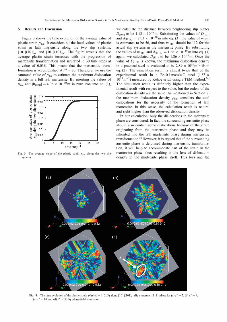
Figure 3 shows the time evolution of the average value ofplastic strain pave. It considers all the local values of plasticstrain in lath martensite along the two slip systems,½101�ð�101Þ¡0 and ½�101�ð101Þ¡0 . The figure reveals that theaverage plastic strain increases with the progression ofmartensitic transformation and saturated in 30 time steps ata value of 0.036. This means that the martensitic trans-formation is accomplished at t* = 30. Therefore, we use thesaturated value of pave to estimate the maximum dislocationdensity in a full lath martensite. By inserting the values ofpave and «b(101)« = 4.06 © 10¹10m in pure iron into eq. (1),

we calculate the distance between neighboring slip planesD(101) to be 1.13 © 10¹8m. Substituting the values of D(101)

and dð101Þ¡0 = 2.03 © 10¹10m into eq. (3), the value of m(101)

is estimated to be 56, and thus m(111) should be 112 for theactual slip systems in the martensite phase. By substitutingthe values of m(111) and dð111Þ¡0 = 1.66 © 10¹10m into eq. (3)again, we calculated D(111) to be 1.86 © 10¹8m. Once thevalue of D(111) is known, the maximum dislocation densityin a practical steel is evaluated to be 2.89 © 1015m¹2 fromeq. (2). The simulation result is almost twice that of theexperimental result in a Fe­0.1mass%C steel (1.55 ©1015m¹2) measured by Kehoe et al. using a TEM method.24)

The simulation result is definitely higher than the exper-imental result with respect to the value, but the orders of thedislocation density are the same. As mentioned in Section 2,the maximum dislocation density μlim considers the totaldislocations for the necessity of the formation of lathmartensite. In this sense, the calculation result is naturaland right higher than the observed dislocation density.

In our calculation, only the dislocations in the martensitephase are considered. In fact, the surrounding austenite phaseshould also contain some dislocations because of the strainoriginating from the martensite phase and they may beinherited into the lath martensite phase during martensitictransformation.5) However, it is argued that if the surroundingaustenite phase is deformed during martensitic transforma-tion, it will help to accommodate part of the strain in themartensite phase, thus resulting in the loss of dislocationdensity in the martensite phase itself. This loss and the

Fig. 3 The average value of the plastic strain pave along the two slipsystems.

A

Fig. 4 The time evolution of the plastic strain p¡i ðrÞ (i = 1, 2, 3) along ½�101�ð101Þ¡0 slip system at {111} plane for (a) t* = 2, (b) t* = 4,

(c) t* = 10 and (d) t* = 30 by phase-field simulation.

Prediction of the Maximum Dislocation Density in Lath Martensitic Steel by Elasto-Plastic Phase-Field Method 1601

dislocations stored in the surrounding austenite phase canceleach other out. Therefore, the maximum dislocation densityin a full martensite should be almost equal to our result.In other words, during martensitic transformation, the totalstrain containing the surrounding austenite phase is consid-ered to be represented by the dislocations in this study,although the quantitative evaluation should be done in thefuture.

Figures 4 and 5 show the time evolution of the local plasticstrain p¡

i ðrÞ (i = 1, 2, 3) along the ½101�ð�101Þ¡0 slip systemand the ½�101�ð101Þ¡0 slip system on the {111} plane byphase-field simulation, respectively. In Figs. 4 and 5, thedeep blue areas indicate that there are no slip deformation,while the red areas represent the most dramatic slipdeformation. For a specific value shown in Figs. 4 and 5,it may come from an arbitrary lattice corresponding in Baindeformation, where the value of i can be equal to 1, 2 or 3.But all the values distributed in a packet contain the localplastic strain for all the three cases of lattice corresponding,i.e., i = 1, 2 and 3. Because of a dislocation loop set in thecenter of the austenite phase as the initial state, the slipdeformation also originated from the center of the austenitephase and the range of the slip deformation extends with theevolution of the martensitic transformation. It is to be notedthat the plastic strain of area “A” marked in Fig. 4(d) is verylarge, while in the same area “B” marked in Fig. 5(d), thereis almostly no plastic strain along the other slip system.This result can be observed at all times and places bycomparing Figs. 4 and 5. So it is concluded that the slip

deformation along the two slip systems are complementaryand they cooperated with each other to assist the plasticaccommodation.

6. Conclusions

The maximum dislocation density of lath martensite in aFe­0.1mass%C steel was evaluated on the basis of a TTSDmodel. By employing an elasto-plastic phase-field methodbased on the TTSD model, the average value of plastic strainwas evaluated to be approximately 0.036 for 30 time steps.The evaluated maximum dislocation density was 2.89 ©1015m¹2. This result was reasonable to be higher than theobserved dislocation density in value but to be the same inorder.

REFERENCES

1) G. Olson and W. Owen: Martensite, (ASM International, MaterialsPark, Ohio, 1992).

2) K. Otsuka and C. M. Wayman: Shape Memory Materials, (CambridgeUniversity Press, Cambridge, 1999).

3) K. Wakasa and C. M. Wayman: Acta Metall. 29 (1981) 973­990.4) K. Wakasa and C. M. Wayman: Metallography 14 (1981) 49­60.5) B. P. J. Sandvik and C. M. Wayman: Metall. Trans. A 14 (1983) 809­

822.6) P. M. Kelly: Mater. Trans., JIM 33 (1992) 235­242.7) D. J. Rowenhorst, A. Gupta, C. R. Feng and G. Spanos: Scr. Mater. 55

(2006) 11­16.8) S. Morito, X. Huang, T. Furuhara, T. Maki and N. Hansen: Acta Mater.

54 (2006) 5323­5331.

B

Fig. 5 The time evolution of the plastic strain p¡i ðrÞ (i = 1, 2, 3) along ½101�ð�101Þ¡0 slip system at {111} plane for (a) t* = 2, (b) t* = 4,

(c) t* = 10 and (d) t* = 30 by phase-field simulation.

Z. Cong, Y. Murata, Y. Tsukada and T. Koyama1602

9) S. Morito, H. Tanaka, R. Konishi, T. Furuhara and T. Maki: Acta Mater.51 (2003) 1789­1799.

10) S. Morito, I. Kishida and T. Maki: J. Phys. IV France 112 (2003) 453­456.

11) S. Morito, H. Saito, T. Ogawa, T. Furuhara and T. Maki: ISIJ Int. 45(2005) 91­94.

12) S. Morito, J. Nishikawa and T. Maki: ISIJ Int. 43 (2003) 1475­1477.13) Z. Cong and Y. Murata: Mater. Trans. 52 (2011) 2151­2154.14) K. Iwashita, Y. Murata, Y. Tsukada and T. Koyama: Phil. Mag. 91

(2011) 4495­4513.15) F. R. N. Nabarro: Phil. Mag. 42 (1951) 1224­1231.16) N. Zhou, C. Shen, M. Mills and Y. Wang: Phil. Mag. 90 (2010) 405­

436.17) A. Yamanaka, T. Takaki and Y. Tomita: Mater. Sci. Eng. A 491 (2008)

378­384.18) Y. Wang and A. G. Khachaturyan: Acta Mater. 45 (1997) 759­773.19) A. G. Khachaturyan: Theory of Structural Transformations in Solids,

(John Wiley and Sons Inc., New York, 1983).20) W. Zhang, Y. M. Jin and A. G. Khachaturyan: Acta Mater. 55 (2007)

565­574.21) Y. M. Jin, A. Artemev and A. G. Khachaturyan: Acta Mater. 49 (2001)

2309­2320.22) J. Kundin, H. Emmerich and J. Zimmer: Phil. Mag. 90 (2010) 1495­

1510.23) Japan Institute of Metals: Metals data book, third ed., (Maruzen, Tokyo,

Japan, 1993).24) M. Kehoe and P. M. Kelly: Scr. Metall. 4 (1970) 473­476.

Prediction of the Maximum Dislocation Density in Lath Martensitic Steel by Elasto-Plastic Phase-Field Method 1603