Prediction of ﬁnancial bubbles and backtesting of a ...

MASTER THESIS

IMPERIAL COLLEGE LONDON

DEPARTMENT OF MATHEMATICS

Prediction of financial bubbles andbacktesting of a trading strategy

Authors:Marc Jeremy

Date: September 2020

Declaration

The work contained in this thesis is my own work unless otherwise stated.

Signature and date:

Jeremy Marc,September 8, 2020

2

Abstract

In our modern society financial bubbles often entail dramatic consequences. Inour research, we focused on defining a financial bubble by drawing from differenttheories. Our work concentrates on the Log Periodic Power Law Singularity modelwhich characterises a bubble as an faster-than-exponential unsustainable growthof the price-time series, which always ends up on a financial crash. After definingthe model theory, its calibration, and describing how one can generate indicatorswith this model, we used it to reproduce some well-known results of the litera-ture. We reproduced the analysis of the bubble in the Chinese stock market SSECin 2014 and 2015. Being able to predict a bubble, we then focused on implement-ing a trading strategy using the LPPLS model. Thereafter, we propose a strategywhich invests when the LPPLS Confidence indicators detect a positive bubble andwhen the LPPLS Trust indicators detects a negative bubble about to crash. Thestrategy is then tested over different classes of assets and financial bubbles. Asa result, our analysis proves the efficiency of the methodology. Furthermore, weenhance the strategy by adding different features, leaving the market when weget a strong positive LPPLS Trust indicator signal. We finally add an Average TrueRange strategy to do size the trades and then adjust the position in matter of themaximal loss we can accept. The studies have been conducted on different as-sets, however, cryptoccurencies and especially Bitcoin is often used to describe thestrategies throughout this work.

3

Acknowledgments

I would like to express my gratitude to Jose Forero and Alexey Gurov, for theirsupport, availability, and trust, and for passing on their knowledge which greatlycontributed to this experience.

I would like to thank all the staff of Velador Associates for their welcome and kind-ness during this internship.

I would like to express my sincere gratitude to my tutor Pietro Siorpaes for his assis-tance and support for this master thesis. I would also like to thank all the teachingstaff of the MSc Mathematics and Finance for the quality of the lectures they deliv-ered throughout the year.

My last thanks goes to my friends and family who helped and supported me notonly throughout this work but through my whole studies.

4

CONTENTS CONTENTS

Contents

1 Introduction 6

2 Bubbles and LPPLS model 92.1 Literature review . . . . . . . . . . . . . . . . . . . . . . . . . . . . . 92.2 Log-Periodic Power Law Singularity model . . . . . . . . . . . . . . . 112.3 Estimation and Calibration of the model . . . . . . . . . . . . . . . . 142.4 LP-AR(1)-Garch(1,1) model . . . . . . . . . . . . . . . . . . . . . . . 172.5 The 2-step/3-step ML approach . . . . . . . . . . . . . . . . . . . . . 182.6 LPPLS indicators . . . . . . . . . . . . . . . . . . . . . . . . . . . . . 19

2.6.1 DS LPPLS indicators . . . . . . . . . . . . . . . . . . . . . . . 192.6.2 Multi-scale indicators . . . . . . . . . . . . . . . . . . . . . . 20

3 Trading strategy 223.1 Generate the LPPLS indicators . . . . . . . . . . . . . . . . . . . . . . 223.2 The trading strategy . . . . . . . . . . . . . . . . . . . . . . . . . . . 26

3.2.1 The strategy . . . . . . . . . . . . . . . . . . . . . . . . . . . . 273.2.2 Literature results . . . . . . . . . . . . . . . . . . . . . . . . . 283.2.3 Visualisation of the results . . . . . . . . . . . . . . . . . . . . 293.2.4 Holding period . . . . . . . . . . . . . . . . . . . . . . . . . . 303.2.5 Results . . . . . . . . . . . . . . . . . . . . . . . . . . . . . . . 31

3.3 The improved strategy . . . . . . . . . . . . . . . . . . . . . . . . . . 383.3.1 The improved strategy . . . . . . . . . . . . . . . . . . . . . . 383.3.2 Holding period . . . . . . . . . . . . . . . . . . . . . . . . . . 393.3.3 Results . . . . . . . . . . . . . . . . . . . . . . . . . . . . . . . 403.3.4 ATR . . . . . . . . . . . . . . . . . . . . . . . . . . . . . . . . 44

4 Conclusion 48

5

1 INTRODUCTION

1 Introduction

Financial bubbles are not a modern conception of an irrational rise of the prices,actually, they are almost as old as mankind. As long as there is a market with a fewconsumers willing to invest their money in a product that seems to have potentialhigh profits in a long or short term, a bubble could potentially appear.

Figure 1: Anonymous 17th-century watercolor of theSemper Augustus, famous forbeing the most expensivetulip sold during the tulip ma-nia

In the early 17th century, in the Netherlands the ex-ceptional development of trades brought the first tulipsbulbs. The tulips were different from any other flowerknown at that moment in Europe. It quickly became asymbol of social status. The tulips were then seen asbeautiful, exotic and a display of good taste. The richmerchants in the Netherlands, at the time, would buytulips as they did with paintings or other rare items.The fast expanding of wealth in the country had mademore people able to buy luxuries. On the other hand,tulips were still very hard to cultivate, which madethem a quite rare object. This scarcity rose the pricesover the years. To understand it, it is important to no-tice that the tulips were under the form of a bulb fromJune to September, making the trades easier. Most ofthe trades were then done on this short period of time.However, outside this lapse of time the Dutch createdcontracts to buy tulips for the next season (effectivelyfutures contracts). As a result, the prices started to ex-plode in November 1636 without any rational reasondespite the avidity of the buyers that would buy at anyprice expecting to sell at an ever higher one. At thattime a bulb could be sold at more that a yearly paidfor a skilled craftsmen, and for the rarest bulb it couldreach the price of a common house. In February 1637,the prices collapsed drastically after an uncertainty in the market, the buyers werenot certain that the prices would still go up, which ended up on a crash. This wasthe first financial bubble ever recorded, and was later called the Tulip mania.

6

1 INTRODUCTION

Figure 2: Anonymous painting ofa debate in the South Sea CommonHouse

In 1711 in England, the South Sea Company lent7 million pounds to the government to financethe war against France. In exchange the SouthSea Company obtained a monopoly in trade withthe South America, which was then under Span-ish and Portugal domination. The company thenbankrolled the English National debt with itsshares, the stocks were delivered and backed withthe national bond and would then deliver a yearly5 percent interests directly from the government.The possible huge profit that would result of thetrades with the Spanish colonies brought manyinvestors in the market, and the prices increasedexponentially. But it was brief, in 1720 a crashhappened, putting back the prices just above itsoriginal price. Additionally, that the companydid not even manage to trade anything with thecolonies, and the prospect was still even unlikelyfrom the beginning. This episode was later calledThe South Sea Bubble, and it ruined many ambi-tious investors.

In these two historical instances we identify some interesting points about bubbles.During a bubble, prices of the asset evolve and move away from what it is calledtheir fundamental value. In a positive bubble, there is an excessive demand, andprices go up. In a negative bubble there is an excess of selling, and prices go down.

Even though these historical events are full of information to define a bubble, finan-cial bubbles are not limited to our past. Many major bubbles have developed in ourmodern society. We could cite the Dot-Com Bubble, for example. As in the historicalexamples, the expectation of huge profits gathered many investors around internetrelated stocks, creating a bubble which crashed in 2000.

Finally, the Tulip Mania, the South Sea Company bubble, or the Dot-Com bubble,share common factors. We observe that a bubble starts with a new opportunity orfuture profit expectation. The nature of the opportunity does not matter in the firstpoint, it could be a new technology, a new class of asset, or even a technical tradingevent. What matters is the prospect of high profits in the future. With this prospectof profits, the investors will start to show interest. The demand for the asset willincrease which will, as well, increase the prices. The positive feedback mechanismthen accelerates the process, the investors would be willing to follow the herd andbuy for higher prices expecting to sell for even more. At that time, the regime inplace can be shaken by any uncertainty in the market, the uncertainty will then gaininvestors, and in a matter of days or even hours everyone will be willing to sell.Prices will drop, and finally produces a financial crash. ’By nature, a bubble is anunsustainable process in which the system is gradually pushed towards criticality’ in

7

1 INTRODUCTION

Sornette & Cauwels (2014). Besides in a critical system, even a small event can havea huge impact, as stated in Sornette & Cauwels (2014), it is not that important tounderstand what was the last event that caused the crash as it was bound to happen,the criticality of the system is what matters most.

In the first section of this thesis, we will review the different theories of the liter-ature to predict a financial bubble. Thereafter, we will focus on the LPPLS model,its calibration, and indicators. In the second part of the thesis, we will propose atrading strategy using the LPPLS model and its indicators. Through this section wewill improve the methodology and analyse the performance of our strategy.

8

2 BUBBLES AND LPPLS MODEL

2 Bubbles and LPPLS model

2.1 Literature review

Detecting financial bubbles in the stock market has always attracted people. Notonly for the academics trying to predict them, but also for the governments seekingto protect their national economy, and for individuals and entities whose daily lifewould be directly impacted by a financial crash.

The dividend discount model introduced first in Gordon & Shapiro (1956) has playedan important role to explain the behavior of bubbles in the stocks market for the re-searchers. Indeed in theory, the dividend discount model make the assumption thatthe present discounted value of the future expected profits determines the stockprices, see Campbell & Shiller (1987). Assuming that we have a time-invariant dis-count rate, and that stock prices and dividends can be modelled as integrated pro-cesses of order one, then dividend discount model predicts an equilibrium betweendividends and stock prices.

Using the theory of the dividend discount model, some academic studies have beencarried out aiming to predict a financial bubble since Diba & Grossman (1988a),notably using the co-integration framework and the unit root. To predict a finan-cial bubble in the stock market, Diba & Grossman (1988a,b) were then looking atthe logarithm of the dividend yield, and if this one followed a stationary or mean-reverting process, they assumed that it was not a bubble. But it is worth noticingthat many other studies state that even if prices and dividends tend on a long termto follow the same pattern, an irregularity or variation can emerge Froot & Obstfeld(1991), and more recently Balke & Wohar (2002), and then such irregularities couldappear by non-linear dynamics in the relation between prices and dividends, an ideaintroduced in Campbell et al. (1997).

It is rather difficult to find an explanation for those non-linearity, indeed it doesmuch probably come from a gathering of different effects.As a first cause of non-linearity, we could state the presence of financial bubbles cre-ated by speculation Blanchard & Watson (1982), and Charemza & Deadman (1995).Furthermore, in Evans (1991) it was proved that the weakness of unit root tests fordetecting periodically collapsing bubbles due to non-linearity. And in Charemza &Deadman (1995), the authors demonstrated (with a simulation analysis) the resultsof the previous study Evans (1991). Secondly, the effect of the noise traders is rele-vant as well to explain the non-linearity, along with the presence of intrinsic bubbles,and the transaction costs.

There exist a lot of studies who focused on detecting the non-linearity in the stockmarket to detect bubbles. Over the years some methods proved themselves quite use-ful and accurate in the prediction while others deprecated over more recent models.

There is in the financial bubble theory a lot of different field of research. To the

9

2.1 Literature review 2 BUBBLES AND LPPLS MODEL

best of my knowledge, we can distinguish three major different streams. The firstone is the one trying to detect bubbles using statistical tests that is best performedby the supremum augmented Dickey-Fuller tests (ADF) in Phillips et al. (2011). Thesecond is a completely separated theory of literature, also very productive, that usesthe fitting of a Log Periodic Power Law (LPPL) to predict a financial bubble that wasfirst introduced in Sornette et al. (1996) .The third is the stream of research intro-duced by Benth et al. (2013), Protter (2016) that build a mathematical theory offinancial bubbles.

This last branch compared to the other is relatively recent but already brings upsome interesting results. Precisely, in this theory, we model the price dynamic of afinancial asset by a continuous stochastic model. We then observe a financial bubblewhen if the stochastic process turns out to be a strict local martingale under the riskneutral measure. A generalised framework has then been proposed in Cretarola &Figa-Talamanca (2019) where we consider that the stochastic process of the priceof the asset is correlated to the stochastic process of the market attention on theasset. This idea allow to capture the positive feedback cycle that boost the price ofa bubble when the market attention grows, under some hypothesis. This researchstream has been applied essentially to criptocurrencies, especially on Bitcoin, Cre-tarola & Figa-Talamanca (2019) proved that Bitcoin boost in a bubble if and only ifthe correlation between changes in price and the attention factor is above a specificpositive threshold. As it is a relatively new stream of research, although academicshave started to put a lot of attention on criptocurrencies these last few years, andthe interest does not seem to fade yet. In Cretarola & Figa-Talamanca (2020) theauthors focused on predicting the bubble regimes in Bitcoin and Ethereum, and in-terpret the correlations between criptocurrencies using the theory of Protter (2016)and Cretarola & Figa-Talamanca (2019). To get those results, they used a continu-ous latent markov chain to model the change of state, and proposed an estimationprocedure using conditional maximum likelihood.

However the main streams of bubble detection resides in the first two branchesdescribed before. Around the statistical methods, there is a lot of techniques that arepopular in the literature, but we will not enumerate nor describe them all in this re-view. To state a few, the momentum threshold autoregressive test (MTAR) of Enders& Granger (1998), the exponential smooth transition autoregressive test (ESTAR) ofKapetanios et al. (2003). At the moment, the supremum augmented Dickey-Fullertests (ADF) is the statistical test providing the best results. This test has been im-porved over the years, with the recursive test (SADF) Phillips et al. (2011), and ageneralised version (GSADF) in Phillips et al. (2015). However this test possessessome drawbacks, one would be assuming cointegration between the dividends andthe prices.

The second stream of literature on financial bubbles resides in the Log PeriodicPower Law Singularity (LPPLS), a theory that has initially been introduced in Jo-hansen et al. (2000), Sornette (2009), Sornette et al. (1996). Under some assump-

10

2 BUBBLES AND LPPLS MODEL 2.2 Log-Periodic Power Law Singularity model

tions it is possible to demonstrate that the prices dynamic follow a LPPLS model.This model improves the traditional definition of a bubble and define it with an al-ternative way. More exactly, instead of seeing bubbles by a chaotic exponential risetill the critical time of the crash, this view characterises the bubble with a faster-than-exponential growth of price conducting to an unsustainable regime that alwaysend up on a crash. The positive feedback is responsible of the bubble, and leadsto the unsustainable regime. And this feedback is created by many factors, such asthe imitation process and herding behaviour of traders. The LPPLS model is then avery powerful tool which by working on the price-time series of an asset is able topredict the critical time of the crash of a bubble. Since the work of Sornette manyothers have used the model to predict the crashes of the major bubbles over the lastdecades, from these numerous studies, we can state the study of the 2000-2003 realestate bubble in the UK Zhou & Sornette (2003), or the post mortem analysis of the2015 Shanghai stock market bubble Sornette et al. (2015).

The LPPLS model has aroused much interest over the last two decades, and proba-bly even more after the crash of the US housing-market bubble. This infatuation ofacademics and researchers on this model, after the crash, has allowed a few inter-esting improvements of the method. In Geraskin & Fantazzini (2013) the authorsreview the LPPLS original model and answer some critics about it, then they pro-posed a new methodology to fit the model and detect a financial bubble with realtime data, after applying it to the gold bubble that crashed in December 2009. Asimple transformation of the LPPLS formulation has allowed to reduce slightly thenumber of nonlinear parameters in Filimonov & Sornette (2013), making a stableand robust calibration of the model. A few studies on the reliability of the beginningand end time of a bubble have also been conducted in Demos & Sornette (2017),this study revealed that it is in fact easier to detect the start of a bubble than its end.In Demirer et al. (2019) the authors examine the predictive power of a few indica-tors derived directly from the LPPLS model, via a multi-scaling method that aim togenerate a confidence indicator revealing the number of time the model predictedthe same bubble over different scale of windows.

2.2 Log-Periodic Power Law Singularity model

This section aims to cover the theory behind the LPPLS model.

The LPPLS model can be see as an extension of the Blanchard & Watson (1982)rational expectation bubble model. A financial bubble is created by a faster-than-exponential growth of price, that conducts to an unsustainable regime that alwaysend up on a crash. The LPPLS model is finally a combination of (i) mathematical andstatistical physics of phase transitions, (ii) behavorial finance, imitation and herdingof traders that creates positive feedback, (iii) the economic theory of bubbles.

In Johansen et al. (2000), Sornette et al. (1996) the model was developed underthe following assumptions

11

2.2 Log-Periodic Power Law Singularity model 2 BUBBLES AND LPPLS MODEL

• The asset pays no dividend

• The risk free asset pays zero interest rate

• Markets clear automatically without the need of imposing any conditions

• The agents are risk neutral

In a bubble phase, for an asset with a given fundamental value, the price trajectoryof the asset, the JLS model Johansen et al. (2000) assumes that the logarithm of theasset price p(t) follows:

dp

p= µ(t)dt + σ (t)dW − kdj (1)

where µ(t) is the expected return, σ (t) is the volatility, dW is the infinitesimal incre-ment of a standard Wiener process, k is the loss amplitude of a possible crash, anddj represents a discontinuous jump with the value of 0 before the crash and 1 afterthe crash.

The LPPLS model considers two different types of agents. The first type consistsof traders that act with rational expectation as in Blanchard & Watson (1982). Thesecond group is made of noise traders that act with behaviour, herding behaviour.One of the assumption is that the collective behaviour of the noise trader is able todestabilize the asset prices via their trades. In Johansen et al. (2000), the authorssuggested that their behaviour could be included in the crash hazard rate h(t), whichis the probability that a crash will occur at a given time point t. It is proportional tothe expectation of dj, we get h(t) = E[dj]/dt.

We then assume that that the asset price satisfies the rational expectation conditionJohansen et al. (2000) which is equivalent to a martingale condition. We multiplythe equation (1) by p(t) and we take the conditional expectation at time t. The non-arbitrage condition expresses that the expectation of the price increment should benull, then, we obtain:

Et[dp(t)] = µtdt + σ (t)Et[dW (t)]− kdj = 0

which simplifies to:

µt = kh(t) (2)

The, we get that the return is proportional to the crash hazard rate with a factor k.Now if we use (2) in (1) and assuming there is no crash (i.e. dj = 0), we end up ona differential equation with solution:

E[ln(ptpt0

)] = k∫ t

t0

h(x)dx (3)

This equation demonstrates that for to price to follow a martingale process, the pricehas to increase along with the crash probability, and higher is the crash probability,

12

2 BUBBLES AND LPPLS MODEL 2.2 Log-Periodic Power Law Singularity model

the faster the price has to increase. This can be explained by the fact that an investorhas to get a higher profit from a more risky asset. Then the price growth follows thecrash hazard growth.

Johansen et al. (2000) suggested that the behavior of the noise traders could bemodelled writing the crash hazard h(t) in this way:

h(t) = α(tc − t)m−1(1 + β cos(ω ln(tc − t)−Φ)) (4)

where α,β,ω,Φ, and tc are the model parameters. The power law singularity residesin the term α(tc − t)m−1 it is the term that models the positive feedback mechanismthat eventually leads to the creation of the bubble. And the log-periodic large scaleoscillations are the two terms of the equations that accounts for the cascades ofoscillations. The log periodic oscillations can be seen as the tension between thedifferent agents of the model, this tension creates deviations in the prices growth,and become more important as we get to the critical point tc.

By combining (4) and (2) substituting with (3), we finally get:

E[lnp(t)] = A+B(tc − t)m1+C(tc − t)m cos(ω ln(tc − t)−Φ)) (5)

with A = ln(p(tc) is the logarithmic price at a critical time and B = −kα/m is theamplitude of the power law, it is the increase of the logarithmic price before thecrash. B < 0 represents a positive bubble, and B > 0 represents a negative bubble.We assume 0 < m < 1 this condition ensures the faster-than-exponential growth tillthe critical time tc. Also we have C = −kαβ/

√m2 +ω2 that is the magnitude of the

oscillations, when ω is the pulsation of those oscillations and Φ is a phase parameter.We also can notice that this formulation allows to model the price dynamics beyondtc we then have to replace tc − t by |tc − t|, we then assume a symmetric behavior ofthe log price after the singularity.

13

2.3 Estimation and Calibration of the model 2 BUBBLES AND LPPLS MODEL

Figure 3: Example of LPPLS model following the equation 3, generated using (m,ω,Φ ,A,B,C, tc) = (0.353689,9.154368,2.074608,7.166421,−0.434324,0.035405,530)

Classic positive bubble regimes can be characterised by those parameters B < 0 with0 < m < 1. The first condition as stated before ensures that we are in a positivebubble, that the prices trajectory will follow a faster-than-exponential growth untilwe reach the critical time tc. The condition 0 < m is the condition that ensures thatthe price remains finite at the critical time, while the condition m < 1 does ensurethe existence of the singularity, the peak of the expected log-price diverges at thecritical time.Afterwards, for the fitting method, as well as the optimization and estimation ofthese parameters, we shall refer to Filimonov & Sornette (2013).

2.3 Estimation and Calibration of the model

As it as already been reported in the literature review, one of the most importantwork on the LPPLS model resides in Filimonov & Sornette (2013), particularly for theestimation and calibration. Their work rewrites (5) by modifying the term C cos().The two parameters C and Φ are then replaced by two other linear parameters thatare always referred as C1 and C2 with C1 = C cosΦ and C2 = C sinΦ. By this change,we do reduce the number of nonlinear parameters in our model, from 4 non linearparameters (ω,m,tc,Φ), we then only have 3 to determine (ω,m,tc). On the otherside we then have more linear parameters to determine, (A,B,C1,C2). Finally we

14

2 BUBBLES AND LPPLS MODEL 2.3 Estimation and Calibration of the model

come from these set of 7 parameters to determine (ω,m,tc,Φ ,A,B,C) to these set of7 parameters (ω,m,tc,A,B,C1,C2).We can now rewrite (5) in terms of our new parameters following Filimonov &Sornette (2013). We then obtain:

E[lnp(t)] = A+B(tc− t)m+C1(tc− t)m cos(ω ln(tc− t))+C2(tc− t)m sin(ω ln(tc− t)) (6)

In order to give an estimation to these parameters, we will use the L2 norm whichgives the following, using the least-square method with the cost function F:

F(ω,m,tc,A,B,C1,C2) =N∑i=1

[lnp(τi −A−B(tc − τi)m

−C1(tc − τi)m cos(ω ln(tc − τi)) +C2(tc − τi)m sin(ω ln(tc − τi))]2 (7)

We can separate the 4 linear parameters from the 3 non linear parameters, we thenget a non linear optimization problem:

(ω, m, tc) = arg minω,m,tc

F1(ω,m,tc) (8)

where the cost function F1(ω,m,tc) is:

F1(ω,m,tc) = minA,B,C1,C2

F(ω,m,tc,A,B,C1,C2) (9)

Similarly to the work of Filimonov & Sornette (2013), the optimisation problem of(9) has a unique solution that is obtained in solving the matrix equation:

N∑fi

∑gi

∑hi∑

fi∑f 2i

∑figi

∑fihi∑

gi∑figi

∑g2i

∑gihi∑

hi∑fihi

∑gihi

∑h2i

ABC1

C2

=

∑yi∑yifi∑yigi∑yihi

(10)

where:

fi ≡ (tc − τi)mgi ≡ (tc − τi)m cos(ω ln(tc − τi))hi ≡ (tc − τi)m sin(ω ln(tc − τi))

(11)

According to Filimonov & Sornette (2013), the modification of the LPPLS equationdelivers two very important results.

First, we notice that the non linear optimisation is transformed from a 4 dimen-sional space to a 3 dimensional one, a modification that significantly reduces thecomplexity of out problem.

Second, the modification wipes out the Φ parameter of the problem, and by the

15

2.3 Estimation and Calibration of the model 2 BUBBLES AND LPPLS MODEL

same way it does eliminate the periodicity of the cost function. Indeed before thismodification there were multiple minima in the cost function, which required meta-heurestic searches. Then this method is undeniably more convenient, because itdoes not require any heuristic to find the minimum.

covariance matrix adaptation evolution

We observe that the cost function can be in this form computed using local searchmethods, such as Levenberg-Marquardt non linear least square algorithm, as statedin Filimonov & Sornette (2013), or the Nelder-Mead method.However there is numerous different methods to compute the estimation of the non-linear parameters. For example the the covariance matrix adaptation evolution strat-egy (CMA-ES) could be applied to minimise the residuals between the LPPLS modelestimations and the price time series. This method, first introduced in Hansen et al.(2003) and developed after by the same authors, is the evolutionary method themost widely spread and used in the scientific community. The performance of themethod made it one of the best among the other evolutionary methods for real-valued single-objective optimisation. It can be applied to nonlinear and non convexoptimisation problem with search space dimension contained between 3 and 100.We will later on observe that those conditions are respected for our model, and thenthis optimisation can be used in our case. Moreover the main advantage of this min-imisation algorithm resides in its invariance properties, along with the preservationof the order of the objective function value.By comparison to the Levenberg, and Nelder-Mead method, the CMA-ES used tocompute the LPPLS estimation has sometimes a lower computation and a lower rel-ative error.

To calibrate the model, we fit the data using the Ordinary Least Square method. Thenthis fitting provides us with the estimation of our parameters (ω,m,tc,A,B,C1,C2) fora certain window of analysis.We define the window of analysis as following. For each fixed point of data t2 thatwe want to analyse, we take a point t1 such our window (t1, t2) as a length dt = t1−t2varying between two values usually between 30 to 750. The size of our window rep-resents the number of trading days we use to fit our LPPLS model to the price timeseries data, so usually between 30 to 750 trading days. Moreover we can use a stepto decrease the window from the 750 trading days to 30, for example a step of 10would make us fit only one window out of ten and we would only have 71 windowsto analyse for each t2.

Whatever the method we chose to apply to get the estimates of the linear param-eter A,B,C1andC2, we chose the nonlinear parameters to reduce and minimise themean squared error of the resulting LPPLS model, by running a Nelder-Mead forexample Filimonov & Sornette (2013).

Furthermore we use some filtering conditions that will select only a few estima-

16

2 BUBBLES AND LPPLS MODEL 2.4 LP-AR(1)-Garch(1,1) model

tion results of our LPPLS model. This is done to minimise some calibration problemsthat could come up, as well as to avoid the minimisation issue of (5).Those filtering conditions have been gathered over the years empirically, by the manystudies conducted in Jiang et al. (2010), Sornette et al. (2015), Zhou & Sornette(2003). It has also been proved that in certain conditions those filtering conditionscould be lighten. And on the other hand previous calibration on the model enlightenthe importance of these condition on the non linear parameters to remove false pos-itive LPPLS fits that would have found a nonexistent bubble Bree & Joseph (2013),Demos & Sornette (2017).

We need to have m in [0,2] to provide an increasing hazard rate and that the priceseries converge to the the price at the critical time when we time converges to thecritical time.We also have to reject the low estimation of the oscillation pulsation ω. This re-jection aims to avoid any slow oscillation that would try to fit the price time seriestrend. We also reject the highest estimations of ω cause they could be just estima-tion fitting the noise. We then take ω ∈ [2,25] which is an interval often chosenin the literature for these reasons Demirer et al. (2019), Demos & Sornette (2017),Filimonov & Sornette (2013).All the filtering conditions and requirements are gathered in table 1.As a more technical requirement, we also need the matrix (10) to be non-singularand well conditioned.

Item Notation Search space Filtering condition 1 Filtering condition 23 m [0,2] [0.01,1.2] [0.01,0.99]

nonlinear ω [1,50] [2,25] [2,25]parameters tc [t2 − 0.2dt, [t2 − 0.05dt, [t2 − 0.05dt,

t2 +0.2dt] t2 +0.1dt] t2 +0.1dt]Nb oscillations ω

2 ln |tc−t1t2−t | − [2.5,+∞) [2.5,+∞)

Damping m|B|ω|C| − [0.8,+∞) [1,+∞)

Relative error pt−ptpt

− [0,0.05] [0,0.2]

Table 1: Filtering conditions and search spaces of valid LPPLS fits from Sornette et al.(2015)

2.4 LP-AR(1)-Garch(1,1) model

In this section, we will introduce a generalisation of the LPPLS model.We already proposed the original LPPLS model, and its estimation and calibration.However, while the original LPPLS is capable of modelling the long range dynamicsof price movements, it is sometimes harder to model the short term price movementwith this model. In Gazola et al. (2008), the authors proposed the following Log-

17

2.5 The 2-step/3-step ML approach 2 BUBBLES AND LPPLS MODEL

Periodic-AR(1)-Garch(1,1) Model:

E[lnp(t)] = A+B (tc − ti)β +C (tc − ti)β cos[w ln(tc − ti) +φ] +uiui = ρui−1 + ηiηi = σiεi , εi ∼N (0,1)

σ2i = α0 +α1η

2i−1 +α2σ

2i−1

(12)

where εi is a standard white noise, which satisfies E[εi] = 0 and E[ε2i ] = 1. And theconditional variance σ2

i follows a GARCH(1,1) process.

The next section will give a new approach to calibrate this Log-Periodic-AR(1)-Garch(1,1) model.

2.5 The 2-step/3-step ML approach

The estimation of the LPPLS model is, in general, never an easy or trivial task toachieve. For example, the presence of local minima in the cost function can eventu-ally ’trap’ the minimization algorithm.

The method we depicted in the previous section is the first one that has been de-veloped and is often referred as a reference, however some alternatives do exist.And these alternatives are sometimes a good help to avoid the computation of theNonlinear Optimization.

In Fantazzini (2010), the authors found out that estimating the LPPLS model overa negative bubble was even easier than for a classical positive bubble. What theycalled an anti-bubble is a negative bubble, the symmetric of a positive bubble. Theprice-time series decreases with log-periodic oscillations to a rebound at the criticaltime.

We have already seen, while establishing the model, that the original LPPLS modelis defined by a stochastic random walk component with an increasing variance. Theidea of the authors in Fantazzini (2010) was to minimise the effect of non-stationarycomponent of the model in reversing the original price-time series (getting a nega-tive bubble instead of a positive bubble).

A first technique was then developed in Fantazzini (2010) called the 2-step ML ap-proach, in order to estimate the LPPLS models using the (12) model. There are thetwo steps:

1. Reversing of the price-time series, and estimation of the LPPLS model for anegative bubble by using the BFGS algorithm (Broyden, Fletcher, Goldfarb,Shanno), coupled with a quadratic step length method (STEPBT) as in Den-nis Jr (1983).

2. Fixing the parameters of the LPPLS model found in 1, we estimate the param-eters of the short term stochastic component (ρ,α0,α1,α2).

18

2 BUBBLES AND LPPLS MODEL 2.6 LPPLS indicators

When the values of the parameters of the LPPLS model reveal poor, or when the bub-ble is just beginning, the computation can be fasten and eased by using an additionalstep. This method was later called the 3-step ML approach used first in Fantazzini(2010):

1. We reverse of the price-time series, and then we change the time scale esti-mation of the LPPLS model making the first day of observation the day of thecrash. We then estimate the LPPLS parameter for a negative bubble by us-ing the BFGS algorithm (Broyden, Fletcher, Goldfarb, Shanno), coupled with aquadratic step length method (STEPBT) as in Dennis Jr (1983).

2. Fixing the parameters of the LPPLS model found in 1, we use these values asstarting values to estimate all the LPPLS parameters, still using the reversedprice-time series

3. Fixing the parameters of the LPPLS model found in 1, we estimate the param-eters of the short term stochastic component (ρ,α0,α1,α2).

This multiple step estimation possesses a lower asymptotic efficiency than the oneproposed before. However we obtain a drastic improvement in the computation-al/numerical convergence. The improvement in terms of efficiency for small andmedium sized data makes this methodology totally relevant. A simulation study inFantazzini (2010) brings the proof of the benefits of this estimation methodology.

2.6 LPPLS indicators

This section will be focused on the LPPLS indicators that can be generated from themodel. First, we will introduce the DS LPPLS indicators as they have been suggestedin Sornette et al. (2015), and then the multi-scaling LPPLS framework, see Demireret al. (2019).

But first, we recall the difference between a positive and a negative bubble. Fora positive bubble, the prices time series exhibit a faster-than-exponential growth to-wards the critical time tc till its crashes. On the other hand, a negative bubble isthe exact mirror situation over the horizontal axis x −→ −x, we then have a faster-than-exponential decrease wich ends up on a change of regime, a negative crash ora positive price rebound. This is modelled in the LPPLS by the B parameter, if B < 0the bubble is positive, and negative in the case where B > 0.

2.6.1 DS LPPLS indicators

We can now introduce the DS LPPLS Confidence indicator and the DS LPPLS Trustindicator, a feature that was first proposed in Sornette et al. (2015) and after usedand enhanced in Zhang et al. (2016).

19

2.6 LPPLS indicators 2 BUBBLES AND LPPLS MODEL

We define both LPPLS indicators at a time t2 as the the fraction of windows wherewe found a bubble respecting the filtering conditions. If we take the example wherefor each t2 we look for each window (t1, t2) with dt = t2 − t1 between 30 and 750trading days with a step of 10. Then, we have to fit the LPPLS model on each of the71 different windows. If we get 7 different windows with a LPPLS fit that pass thefiltering conditions, we then obtain a confidence indicator of 7/71.A large value of the indicator will then be the signal that a lot of our LPPLS modelhave fitted and pass the filtering condition, we can state in this case that there iswith a high probability a bubble. On the other hand, a small value of the indicatorstates that only a few windows have had a LPPLS that fitted, then it is unlikely thatthere is a bubble.

DS LPPLS Confidence is defined as the fraction of fitting windows for which theparameters of the LPPLS model satisfies the filtering condition 1 in table 1, page 17.It indicates the sensitivity of the bubble at a fixed date of time. A value close to 0will indicate that only a few windows verified the conditions, a value close to 1 willhowever indicate the reverse and that the LPPLS model pattern has been observedmany times, we then have a confidence level in the bubble.

DS LPPLS Trust is the median level over the number of estimations windows ofthe fraction among the number of repetitions that satisfy the filtering condition 2 intable 1, page 17. It indicates how closely the LPPLS model calculated respects theprice-time series. A value close to 0 will indicate that only a few windows whereclose of the price-time series, a value close to 1 will however indicate the reverseand that the LPPLS respects very closely the price-time series, we then have a levelof Trust in the bubble. This level being larger than 5% alerts that the current courseof prices is in a critical state and that a transition will occur.

However with some data we do not need to generate the indicators using the wholespectrum of windows (t1, t2), with dt = t2 − t1 between 30 and 750 trading days. Forsome data, only short term windows would be useful and relevant. We then have todefine Multi-Scale indicators.

2.6.2 Multi-scale indicators

In Demirer et al. (2019) the authors introduced different bubbles indicators relyingon the window size the indicators were computed, a short-term bubble indicator, amedium-term bubble indicator, and a long-term bubble indicator. As explained inthe last section all of the indicators at time t2 are a fraction of the fitting LPPLSmodel over the window and then have values in [0,1].

The short-term bubble indicator is the indicator for the window (t1, t2) of sizedt = t2 − t1 in [30,90]. For example if the fit for a specific window respect thefiltering condition we set its value to 1, if not to 0. If the step we took is equal to 10,

20

2 BUBBLES AND LPPLS MODEL 2.6 LPPLS indicators

we will have 7 different windows to look at ((90−30)/10+1). If we found 2 acceptedfits, we will take the short term indicator as the average of the fits, we would havethere have Shortind = 2/7.

The medium-term bubble indicator is the indicator for the window (t1, t2) of sizedt = t2 − t1 in [90,300]. For example if the fit for a specific window respect thefiltering condition we set its value to 1, if not to 0. If the step we took is equal to10, we will have 22 different windows to look at ((300 − 90)/10 + 1). If we found2 accepted fits, we will take the short term indicator as the average of the fits, wewould have there have Mediumind = 2/22.

The long-term bubble indicator is the indicator for the window (t1, t2) of sizedt = t2 − t1 in [300,750]. For example if the fit for a specific window respect thefiltering condition we set its value to 1, if not to 0. If the step we took is equal to10, we will have 46 different windows to look at ((300 − 750)/10 + 1). If we found2 accepted fits, we will take the short term indicator as the average of the fits, wewould have there have Longind = 2/46.

21

3 TRADING STRATEGY

3 Trading strategy

This part of the thesis is focused on the work I realised during my internship. Unlessstated otherwise, the work contained in this part is my own work.

My work has for final objective to implement a trading strategy and make someprofits out of a financial bubble. In a first time, we have to determine a methodologyto predict bubbles. And in a second time, we have to develop a trading strategy torealise a profit out of the bubble we detected. In my work I focused on the LPPLSmodel, and how one could use it to determine a trading strategy that would be effi-cient on different type of assets.

In a first part, I will describe how I predicted a bubble using the LPPLS model byreplicating a well-known result of the literature. Following these explanations, I willdefine a trading strategy using the LPPLS indicators. Then, we will backtest thestrategy and analyse the results. In this work, a significant number of ideas occurredfrom the observation of my results. Consequently, the last part of this section will befocused on these ideas and features that improved the trading strategy.

But first, we shall generate the LPPLS indicators.

3.1 Generate the LPPLS indicators

The first step is to detect a bubble using the previous theory of the LPPLS model,developed over the years in Johansen et al. (2000), Sornette (2009), Sornette et al.(1996). As described in the last section, following this theory, in a bubble state theprice-time series follows a power law possessing log periodic oscillations, that ulti-mately ends up on a crash.

There exists different ways to compute the LPPLS model and its parameters for anasset, they are all very well explained in Geraskin & Fantazzini (2013). So far, wediscussed the detection of financial bubbles by fitting the LPPLS model, and thenlooking at the quality of the parameters over heuristic results.In this thesis, I first worked with the original studies of the LPPLS model in Johansenet al. (2000), Sornette (2009), Sornette et al. (1996). I developed in python somecode to do the basics task and generate the fitting LPPLS model from the price-timeseries data. After I focused on this specific article Demos & Sornette (2017) to gen-erate the DS LPPLS Confidence and DS LPPLS Trust indicators from part 2.6. Codingfunctions that would generate such indicators was not an easy thing to do and tookme a few weeks. I realised then that computing the indicators was taking too muchtime, indeed using the original theory of LPPLS and computing the optimizationproblem of 10 requires heavy calculations. To compute the LPPLS model and dothe computations using this model, one must dispose of a lot of computation powerwhich I did not at the time. I then decided to move on to another computationalapproach to get my results.

22

3 TRADING STRATEGY 3.1 Generate the LPPLS indicators

In Geraskin & Fantazzini (2013), the authors created a R library that have beenafter improved with the recent discoveries and improvement of the theory over theyears. It does contain numerous function that computes the parameters of the LPPLSmodel following the model introduced at the end of the previous section, equation12, and using the 2-step/3-step aproach to compute the model, in part 2.5. Thelibrary can be found in Fantazzini (2020). The work done in this library is quiteremarkable and it proved itself very helpful for our work in this thesis.

As a first step to use the LPPLS model to detect a bubble, we focused on replicatingthe work done in Sornette et al. (2015), more precisely the work done on the bubbleregime that evolved in the Chinese stock market between mid 2014 and 2015.

Using the LPPLS theory, we look at every single day in the data. For each day t2we look for each window (t1, t2) with dt = t2 −t 1 between 120 and 250 trading dayswith a step of 10. To compute the DS LPPLS Trust indicator, we use a number of10 repetitions. This number is very undervalued compared to the 100 chosen inthe study Sornette et al. (2015). We made that choice of reducing the number ofrepetitions to increase the computing time of our algorithm. This is an issue we willdiscuss later, but it should already be stated that the generating the indicators ofthe LPPLS model is a time-consuming operation that takes hours even days for largedata.In order to alleviate the number of tasks our CPU needs to compute. We do someparallel computing/processing. We need for each time of data t2 to compute the

LPPLS model for250− 120

10+ 1 = 14 different windows. We divide our processor in

7 entities so that for each point of data we can calculate the models in two stepsinstead of 14. However, even with this technique, computing the indicators requiredaround 6 hours for the 3 years of data we had.

We used the data of the SSEC index Chinese stock market between July 2012 toJuly 2015. This is the result we obtained:

23

3.1 Generate the LPPLS indicators 3 TRADING STRATEGY

Figure 4: Computing the DS LPPLS Confidence and DS LPPLS Trust indicators with theSSEC index

Our algorithm return the table in figure 4. It contains all the information about thefitting of the LPPLS model on our data, for every trading day.

• bet: this is the average estimation of the LPPLS parameter β over all the esti-mation windows

• ome: this is the average estimation of the LPPLS parameter ω over all theestimation windows

• phi: this is the average estimation of the LPPLS parameter φ over all the esti-mation windows

• A: this is the average estimation of the LPPLS parameter A over all the estima-tion windows

• B: this is the average estimation of the LPPLS parameter B over all the estima-tion windows

• C: this is the average estimation of the LPPLS parameter C over all the estima-tion windows

• tc: this is the average estimation of the LPPLS parameter tc over all the estima-tion windows

• length: this is the average length over all the estimation windows

• num.osc: this is the average estimation of the number of oscillations over allthe estimation windows

• damping: this is the average estimation of the damping over all the estimationwindows

24

3 TRADING STRATEGY 3.1 Generate the LPPLS indicators

• rel.err: this is the average estimation of the relative error over all the estima-tion windows

• lppl.Confidence: the Confidence indicator as defined in part 2.6

• lppl.Trust: the Trust indicator as defined in part 2.6

• crash.lockin: this is the critical time tc in date format

We have computed in this table all the important information on the computed LP-PLS model for every single day of our data. We notice that do not have any LPPLSConfidence indicator for the year of the data, indeed we computed the model usinga window between 120 and 250 trading days, so the first year (250 trading days)cannot be computed and are referred as Not A Number in our table.

Figure 5: SSEC index in red together with the DS LPPLS Confidence indicator in orangefrom 2012 to 2015

We computed the indicators as Sornette did in Sornette et al. (2015), in taking forlast date, the same that he did. Our results then provide a diagnosis on the bubblethat was forming at this moment in the SSEC index. We do observe a change ofregime in early 2015, at the exact same period they did in their research.However we notice that we get the LPPLS Confidence peak in early 2015 goes to 0.07in Sornette et al. (2015), when in our computation we obtain a peak that reaches upto 0.38. This discrepancy comes from the different technique we used to generate

25

3.2 The trading strategy 3 TRADING STRATEGY

our result.Indeed in Sornette et al. (2015), the authors used the original LPPLS model thatwe introduced in the first part, when we used the 3-step ML approach techniqueintroduced in Gazola et al. (2008). The difference could eventually come from thewindow step we worked with. We took a window step of 10, which means thatwe were looking at only one window of ten. And taking a step of one could haveeventually reduce the peak. Indeed the Confidence indicator, which is the ratio ofthe number of bubble found on the number of windows observed, would have beendivided by a greater number of windows taking 1 as the step. So our high peakcould have resulted from ’some luck’ if a lot of the 10 step away windows containeda bubble for the LPPLS model.

Figure 5 illustrates the DS LPPLS indicator signal for the SSEC index between July2012 and July 2015. It is a rather good example to explain the model. As said be-fore, we observe that the figure do not have any LPPLS Confidence indicator for theyear of the data. Indeed we computed the model using a window between 120 and250 trading days, so the first year could not be computed. This one of the limitationof the model.

3.2 The trading strategy

Now that we are able to detect a bubble, and predict the critical time of its crash,as well as to compute the indicators of early bubble warning and end flag bubble, itwould be relevant to understand how we could use this to make a profit out of it.Academic studies about LPPLS have been really thriving these last few years sincethe outstanding work of Johansen et al. (2000), Sornette et al. (1996). However tothe best of our knowledge there is only a very limited number of papers, articles andstudies that uses these recent discoveries and apply them to build a trading strategyusing the LPPLS model. And all of them have been carried out recently compared tothe year discovery of the LPPLS model.

In our research work, we found an interesting study by Mamageishvili (2019), fo-cused on a trading strategy using LPPLS indicators that we replicated and tested.The strategy relies on the LPPLS confidence indicators, the DS LPPLS Confidencealso called the early bubble warning and the DS LPPLS Trust indicator also calledend flag bubble indicator.

In the following section, I will describe the strategy as I implemented it in my work.It is rather different from Mamageishvili (2019), even if the first idea is quite similar.Indeed in Mamageishvili (2019), they computed the indicators using the original LP-PLS model, and as said in the previous section, in my work I computed the indicatorsusing the 3-step ML method of Geraskin & Fantazzini (2013). The approach I usedcomputes faster but also obtains fewer indicators compared to the original method,I had then to adapt to get an efficient trading strategy.

26

3 TRADING STRATEGY 3.2 The trading strategy

3.2.1 The strategy

If we start from the beginning, the first idea that comes up in our mind is to try toinvest as soon as we detect a bubble and leave the market when this bubble is aboutto crash. The simple idea proposed in Mamageishvili (2019) is to buy the asset ifwe have the signal of an emerging bubble, we can then ’surf’ on the bubble as pricesfollow a faster than exponential trend, and we are out of the bubble when it is aboutto crash. Furthermore, the strategy looks at emerging negative bubble to avoid thedrop in the prices and eventually invest when prices are at the lowest.

First, we recall the idea behind the two indicators we use. The early bubble warningrepresents the apparition of a bubble pattern in the price time series, a positive bub-ble indicator means a positive bubble when a negative one indicates the emergenceof a negative bubble. The end flag bubble indicates that the bubble is matured andis about to crash or to get a noticeable variation. If the indicator is larger than 5%the positive bubble is likely to crash, and if the indicator is below −5% the negativebubble is likely to rebound.

When we get a signal at time t, we trade at time t +1 with the adjourned price.We define two different conditions.The strategy includes short and long time indicators, this is a really important fea-ture that ensure to look at short term bubbles but also for bigger long term bubbles.

First condition:If one of these requirements is fulfilled we enter the market at time t+1.

• LPPLS Confidence short term indicator is larger than a threshold α

• LPPLS Confidence long term indicator is larger than a threshold α

The first one ensures to take profit and hunt for positive bubbles. We take α ∈(−0.1,0.1), this value has to be determined for each specific stock in a way that itoptimises the Sharpe Ratio.

Second condition:If one of these requirements is fulfilled we enter the market at time t+1.

• LPPLS Trust short term indicator is negative

• LPPLS Confidence long term indicator is less than −0.05

This one aims to focus on the end of a negative bubble, to then invest when theprices are about to rebound.

The strategy:

• If the second condition is verified we invest for n2 (depends on the windowsizes used) consecutive days at time t +1

27


• Else if the first condition is verified we invest for n1 (depends on the windowsizes used) day at time t +1

• if none of them, we are out of the market at t+1, we then invest in the risk-free3-Month US Treasury Bills

This strategy differs from Mamageishvili (2019) in many ways.

First, in the definition of the second condition, I decided to implement it with a’or’ instead of a ’and’, if at least one of the requirement is fulfilled I consider thesecond condition to be true. My studies proved this to be more efficient, this is astraightforward improvement that is due to the approach I choose. Indeed I do notobtain as many indicators as in Mamageishvili (2019), and then obtaining a DS LP-PLS Trust indicator negative for both long and short term at the same time is veryunlikely with my approach.

Second, when I invest, I hold my position for a fixed number of days, n1 for thefirst condition and n2 for the second condition. While in Mamageishvili (2019), thestrategy proposed was investing for only one day if the condition 1 for verified, and100 days if the second was.

The performance of the strategy is then compared to the buy and hold strategy.We use the Sharpe Ratio and we compare the Profit and Loss of the strategy againstthe buy and hold.

3.2.2 Literature results

In Mamageishvili (2019), the author performed the strategy over 27 equity indiceslocated in USA, Asia, and Europe, between 1996 and 2018. This lapse of time ofmore than 20 years is really fascinating while hunting for bubbles. As it does con-tain two major equity bubbles: the Dot-Com bubble, and the Subprimes bubble.This strategy outperformed the hold and buy strategy on 22 indices out of the 27tested in their work, with respect to the Sharpe Ratio.

In their work they also conducted a few studies to calibrate the thresholds aroundthe indicators. This calibration revealed very useful in our work but we did notreplicate this studies as it was non essential to get our own results, and was a highlytime-consuming task. However we used the parameters found to compute our strat-egy.

One of the major outcome of the backtesting of this strategy is the following, even asmall indicator is already a good indication of a possible bubble. We then expect tohave as much as indicators as possible to have more trading opportunities. Indeedour indicators represent the number of bubble we saw appearing in our moving win-dows. Hence a small indicator still proves that the LPPLS model found at least one

28


legitimate fitting bubble across our data. Hence it might already be enough to starttrading.

3.2.3 Visualisation of the results

The Sharpe Ratio

We recall the definition of the Sharpe Ratio. It was introduced by William ForsythSharpe in 1966, a Nobel-prize winning economist, who also helped establish theCapital Asset Pricing Model (CAPM). It is used to understand the return of an invest-ment over its risk. The Sharpe Ratio is the average return earned subtracted of therisk-free rate over the total volatility. Subtracting the risk-free rate from our expectedreturns isolate the profit that can be made with risk from the risk free profits. Therisk free rate is the return made from a zero risk investment, here in our strategy it isthe 3-month US Treasury Bill yield. The higher the value, the better the investmentis, compared to the risk.

We resume all of that in the Sharpe Ratio formulation:

SharpeRatio =E[Rp]−Rf

σp

With Rp the return of the portfolio, Rf the risk-free return, and σp the standard vari-ation of the portfolio.

The Sortino Ratio

To observe the results of our strategy I decided to use another indicator, even thoughnone of the studies I worked with used it, I felt this indicator would have a non-negligible value in the analysis of the results, and would complete the Sharpe Ratio.

While computing the efficiency of a strategy, the investor may decide to not pe-nalise a strategy for positive volatility.The Sortino Ratio is a metric that attempts to penalise an asset only with its negativevolatility, by considering the standard deviation of the negative returns instead ofthe deviation of all the returns in the Sharpe Ratio.

How to compute the negative volatility can be debated. But by definition, thestandard deviation of an asset measures the dispersion of the data compared toits average. When we apply the standard deviation definition to negative returns, itmeasures dispersion around the average negative return. However, it is often moreuseful to compute the dispersion compared to a target, usually 0. Like this we mea-sure the dispersion compared to 0. This idea was introduced in Rollinger & Hoffman(2013). In fact the positive volatility means profits, so we are often willing to acceptand concentrate only on the negative volatility. This is the interest of this ratio, thedownside deviation allows to isolate only negative returns of the strategy.

29


We resume all of that in the Sortino Ratio formulation:

SortinoRatio =E[Rp]−Rf

σd

With Rp the return of the portfolio, Rf the risk-free return, and σd the downsidedeviation of the expected return of the strategy. The Sortino Ratio is often preferredto Sharpe Ratio for evaluating high-volatility portfolios, when the Sharpe is morecommonly used for low volatility portfolios. In our case, the combination of the tworatios is interesting, as when during the different states of a bubble, we go throughhigh and low volatility phases.

Along with the Sharpe Ratio, the Sortino Ratio is of great help to compare strategies.

3.2.4 Holding period

We should also comment the number of days we are holding the asset if one ofthe conditions is verified. In Mamageishvili (2019), the author proposed to test thenumber n2 of days we should hold the position when the second condition is veri-fied. The tests have been conducted for n2 in [20,200], and the best results seems tohave been obtained with n equal to 100, all parameters fixed. In my work I decidedto keep this result and work with n2 = 100.

Yet no studies have been carried on the number of days one should hold the po-sition if the first condition is verified.I then decided to run some tests to determine the holding period n1.

I worked with the Bitcoin data over the last 3 years. I run my strategy over the datafor different holding periods, and then compared the Profit and Loss and SharpeRatio of the strategy for the last trading day. This is the results I obtained:

30


Figure 6: P&L and Sharpe ratio of the strategy with variable holding periods, for

We observe that a holding period between 30 to 40 trading days would grant us thebest results in terms of P&L and Sharpe Ratio. This result was partially predictablecause the holding period depends first from the indicators and then from the waywe generated them and specifically the range of windows we took to generate them.In this case, I generated the short term indicators Confidence and Trust using win-dows in [30,90] using a step of 10. For the long term, I first generated the in-dicators Confidence and Trust using windows in [90,250] with a step of 10. Theaverage size of the windows for the long term indicators is then of 170 trading days.And if we refer to the table 1, and our observations, the crash date happen usually0.2× (t2 − t1), where (t2 − t1) = dt is the size of the window, which would give in ourcase 0.2×170 = 34 days later in average. Then we are not surprise to get this result.In this specific case, it seems that the best n1 would be 38 days, in terms of PL andSharpe Ratio.

When one wants to invest in a stock using the strategy, running this test might givea different number for a different asset. Our tests, with different asset classes, alsorevealed that a holding period in [20,50] gives usually good results.

3.2.5 Results

We shall now describe with more details the results obtained with this strategy.

I replicated the strategy over different classes of assets. I carefully selected theassets I worked with, to obtain a coherent set of data across equity, commodities,currencies, and cryptocurrencies. Those choices were motivated by different factors,

31


first it was in the intention of the company to conduct these studies on differenttypes of assets. And more academically, the LPPLS model has been applied to eq-uities in almost all the studies I was able to find. Furthermore it has always beenmy intention to prove that my strategy could be applied on different classes of assets.

However, due to time constraints, we were not able to conduct as many tests onthe strategy as we would have wanted. Indeed, as stated before, computing the LP-PLS indicators takes usually many hours, even days when working on large datasets.

Equity

First, I started by reproducing the strategy on the S&P 500 for the last 25 years.

To apply our trading strategy, we first need to have the LPPLS indicators, DS Con-fidence and DS Trust computed for the whole 25 years of data. In the strategy, wehave to compute two types of indicators, short period and long period indicators.Moreover I noticed that the time period to produce the indicators was not specifiedin Mamageishvili (2019), I then decided to work with the short and long periodindicators as defined in the part 2.6.2. I generated the short term indicators Con-fidence and Trust using windows in [30,90] using a step of 10. For the long term,I first generated the indicators Confidence and Trust using windows in [300,750].This operation was time consuming, it took no less than 4 straight days to computethe long term indicators, even using parallelisation of the processors.

However, I faced an issue while generating the long term indicators with size win-dows in [300,700]. Indeed I did not find any fitting LPPLS bubble with these sizesof windows. This is much probably an issue of the LPPLS model. When trying tofit the model on a lot of data with big windows, we end up finding a fitting modelwith too much relative error. But to accept a LPPLS model, the model has to ful-fill some conditions and pass through the filtering condition of table 1. And withinthose conditions, we have that the relative error must be contained in [0,0.05]. Thenif we work with large windows, the model will have to fit perfectly to get a relativeerror that passes through the error condition. That explains why we did not find anyfitting bubble in that case.

I then decided to work with medium window sizes instead of large, as defined inpart 2.6.2. Using medium term indicators, I successfully generated the Confidenceand Trust indicators.

In the first condition of the strategy in 3.2.1, we should choose the parameter αto optimise the Sharpe Ratio. I computed the model for different values, and I foundthat a threshold α equal to 0 was the best option for the S&P 500.

The results obtained are gathered in figure 8, page 36.

32


The figure 8 contains 5 different charts. The two firsts contain the prices alongwith the indicators found using the LPPLS model, the first one displays the positiveindicators, and the second the negative indicators. The third chart is the ratio ofthe P&L of our strategy over the buy and hold strategy, for every trading day of ourdata. And the last two graphs display the Sharpe and Sortino Ratio of our strategy,compared to the hold and buy strategy.In those graphs we can observe green and red vertical lines. A green line representsa buy, and a red a sell. We always start by buying the stock and we always sell it onthe last trading day if we possess any.I followed this rule with every asset I worked with and kept the same format to dis-play my results.

The first graph proves the efficiency of the LPPLS model to detect a bubble in anasset. We obtained two indicators that predicted the Dot-com bubble emergence in1999. Also the model generated two others at the early stage of the Subprime bub-ble, and again two indicators when the bubble was maturing. However, we observethat we got much more shot term indicators than long term indicators. A result thatcomes from the difficulty to obtain a fitting LPPLS model while working with hugewindows.

The P&L obtained with the strategy is unfortunately lower than the buy and holdstrategy. This can be explained by the time we spent in the stock. Indeed, the LPPLSmodel did not generate enough indicators for us to spend enough time in it andmake profits out of the bubbles.To obtain more indicators we would need to compute the indicators using a shorterstep, and then look at more windows. However in this work I was limited by thecomputational power at my disposal. Indeed, my company gave me an access toan external server, but even with this, computing the indicators usually takes a fewdays. Taking a step of 10 was then a reasonable choice between time constraints andaccuracy.

In terms of Sharpe Ratio, the strategy is performing better than the hold and buystrategy. Furthermore, the Sortino Ratio proves that the strategy performs also bet-ter in terms of negative volatility.

Cryptocurrency

After working on equities, I moved on to cryptocurrencies, this choice was moti-vated by some reasons. First, many cryptocurrencies such at Bitcoin does possessa few interesting bubbles that appeared on quite a short period of time, making iteven easier for my algorithm to compute the indicators. Second, my tutor expressedits interest in that specific class of asset. Moreover I was eager to try out a strategy,that had only been tested on equities (to the best of my knowledge), on a differentclass of asset.

33


First, I worked with Bitcoin (prices in US Dollars) over the last 3 years, from 01/12/2016to 01/08/2020.

I generated the short term indicators Confidence and Trust using size windows in[30,90] using a step of 10. For the long term, I first generated the indicators Con-fidence and Trust using size windows in [90,180] with a step of 20. Having only3 years of data to analyse, it was not relevant to compute the long term indicatorson bigger windows. The data used being quite small, computing the indicators wasmade in a matter of hours for the short term, and a bit more than a day for the longterm, using 7 paralleled processors at a time for each run.

In the first condition of the strategy in 3.2.1, we should choose the parameter αto optimise the Sharpe Ratio. I computed the model for different values, and I foundthat a threshold α equal to 0.05 was the best option for the Bitcoin.

The results obtained are gathered in figure 9, page 37.

To the best of my knowledge, this is the first time that this trading idea was ap-plied to cryptocurrencies.

The results I obtained with the Bitcoin data are excellent and then deserve moreexplanations.

First, we notice that the model generated many indicators, both short and long termindicators. This can be explained by the incredible similarity between the price-timeseries of the Bitcoin and the LPPLS model. We do observe perfect log periodic oscil-lations in the prices of Bitcoin, that lead the asset to an unsustainable growth, anda crash. These similarities explain the huge number of LPPLS indicators, and theiraccuracy.

We are able to detect the beginning of the Bitcoin bubble exceptionally early, inthe first months of 2017, thanks to the LPPLS model. Unfortunately, we do not usethis information to make profit as in this model we proposed a strategy with a fixedholding period n1 and n2 (I recall that we found n1 = 38 in 3.2.4). We also observe agathering of positive indicators when the bubble is about to crash in December 2017.And specifically a DS LPPLS Trust indicator just a few days before the crash, whichexactly means that in a short period of time the bubble will reach its mature stateand a crash will follow. That this specific result that gave me the idea to developa new condition in my strategy that will force the investor to exit the market whensuch an indicator occurs (next part).

The P&L of the strategy exceeds the buy and hold strategy. Indeed the indicators inNovember 2017 gave us a signal to enter the bubble just a month before its crash,and during this month the prices almost doubled. And something quite similar hap-pened during the second bubble of the Bitcoin.

34


In terms of Sharpe and Sortino Ratio, our strategy performs well, we are abovethe buy and hold strategy.

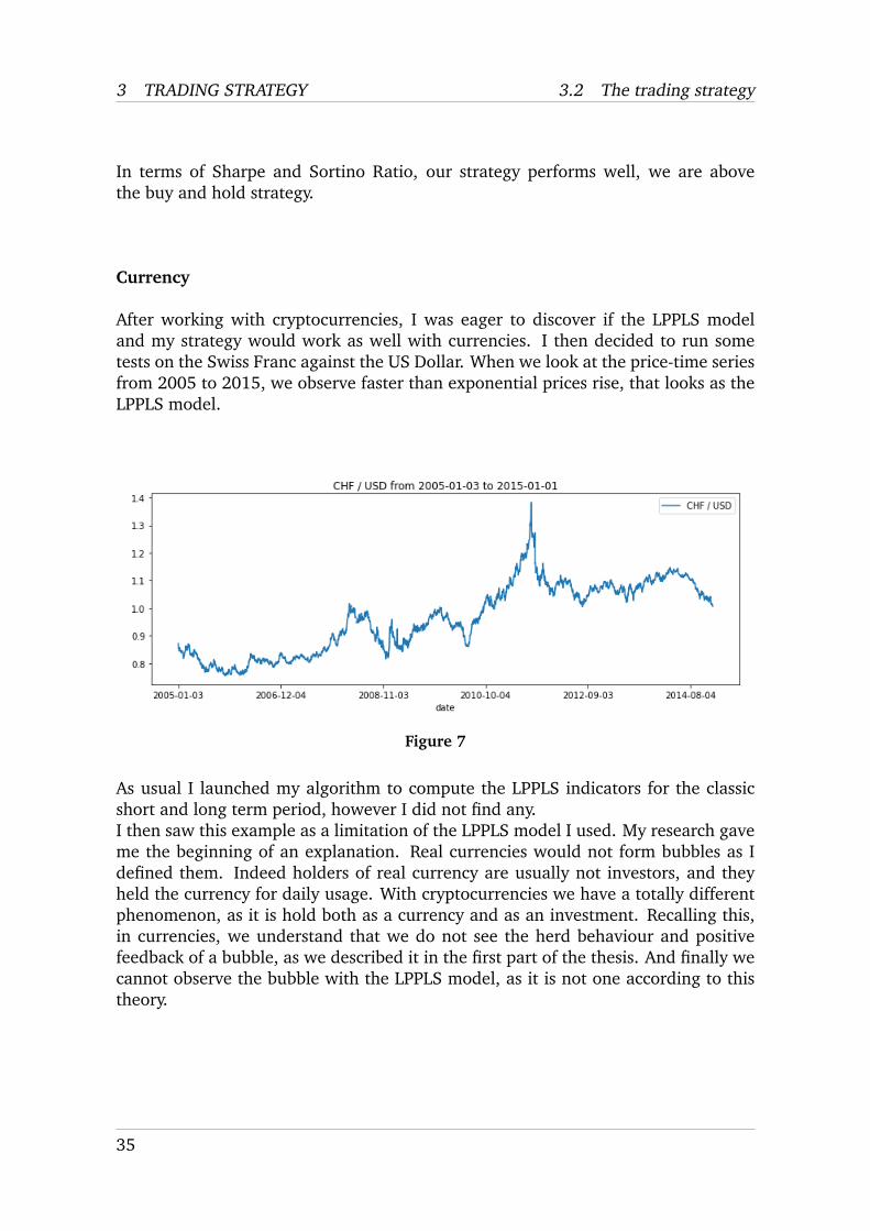
Currency

After working with cryptocurrencies, I was eager to discover if the LPPLS modeland my strategy would work as well with currencies. I then decided to run sometests on the Swiss Franc against the US Dollar. When we look at the price-time seriesfrom 2005 to 2015, we observe faster than exponential prices rise, that looks as theLPPLS model.

Figure 7

As usual I launched my algorithm to compute the LPPLS indicators for the classicshort and long term period, however I did not find any.I then saw this example as a limitation of the LPPLS model I used. My research gaveme the beginning of an explanation. Real currencies would not form bubbles as Idefined them. Indeed holders of real currency are usually not investors, and theyheld the currency for daily usage. With cryptocurrencies we have a totally differentphenomenon, as it is hold both as a currency and as an investment. Recalling this,in currencies, we understand that we do not see the herd behaviour and positivefeedback of a bubble, as we described it in the first part of the thesis. And finally wecannot observe the bubble with the LPPLS model, as it is not one according to thistheory.

35


S&P 500

Figure 8: LPPLS Confidence and Trust indicators and performance of the strategyfor S&P 500 from 1995-12-01 to 2020-05-29. The first two panels illustrate the price-time series and LPPLS Confidence and Trust indicators, the first one displays positiveindicators, and the second negative indicators. The third panel displays the P&L ratio ofour strategy over the buy and hold strategy. The last two panels, Sharpe and Sortino Ra-tio, compare the performance of our strategy (in blue) against the buy and hold strategy(in orange). The green vertical lines indicate that we enter in the market and the redones that we leave the market.

36


Bitcoin

Figure 9: LPPLS Confidence and Trust indicators and performance of the strategyfor Bitcoin from 2016-12-01 to 2020-05-31. The first two panels illustrate the price-time series and LPPLS Confidence and Trust indicators, the first one displays positiveindicators, and the second negative indicators. The third panel displays the P&L ratio ofour strategy over the buy and hold strategy. The last two panels, Sharpe and Sortino Ra-tio, compare the performance of our strategy (in blue) against the buy and hold strategy(in orange). The green vertical lines indicate that we enter in the market and the redones that we leave the market.

37

3.3 The improved strategy 3 TRADING STRATEGY

3.3 The improved strategy

The strategy we used in the previous part performed well in some cases, and gen-erated interesting results. However, from the analysis of these results, I figured outdifferent ways to improve the strategy.

First, I propose to develop the idea we suggested in the previous part, use the pos-itive DS LPPLS Trust indicators as a signal that the bubble will soon crash and thatwe should leave the market.

Second, we did not discuss the quantity we should invest when we enter the market.I then propose to improve the strategy by implementing an ATR risk managementfeature for position sizing, to protect the strategy against a loss, and take the volatil-ity into account.

In my work I computed the strategy across many assets, equity indexes with S&P500 and CAC 40, cryptocurrencies with Bitcoin, Ethereum and others, commoditieswith gold, oil and others, and currencies with the Swiss Franc.In this part, as I cannot describe exhaustively every studies I have undertaken, Iwill focus on cryptocurrencies results, as it does describe perfectly how the strategyworks.

3.3.1 The improved strategy

First condition:If one of these requirements is fulfilled we enter the market at time t+1.

• LPPLS Confidence short term indicator is larger than a threshold α

• LPPLS Confidence long term indicator is larger than a threshold α

The first one ensures to take profit and hunt for positive bubbles. We take α ∈(−0.1,0.1), this value has to be determined for each specific stock in a way that itoptimises the Sharpe Ratio.

Second condition:If one of these requirements is fulfilled we enter the market at time t+1.

• LPPLS Trust short term indicator is negative

• LPPLS Trust long term indicator is less than −0.05

This one aims to focus on the end of a negative bubble, to then invest when theprices are about to rebound.

Third condition:If one of these requirements is fulfilled we enter the market at time t+1.

• LPPLS Trust short term indicator is greater than 0.05

38

3 TRADING STRATEGY 3.3 The improved strategy

• LPPLS Trust long term indicator is greater than 0.05

This one aims to focus on the end of a positive bubble, we then avoid the crash. Athreshold of 0.05 is a good compromise that allows to work only with strong signalsof a possible crash.

The strategy:

• If the third condition is verified we leave the market at time t +1 and we wait50 days to enter again

• Else if the second condition is verified we invest for n2 consecutive days at timet +1

• Else if the first condition is verified we invest for n1 consecutive days at timet +1

It is also important to notice that we do not invest in the 3-Month US Treasury Billsanymore. Even if on a theoretical plan this is a good idea, in practice this actioncould cause liquidity issue, I then decided to compute the results without this lastoperation.

3.3.2 Holding period

As is the previous section, we should comment the number of days we are holdingthe asset if one of the conditions is verified. As the strategy changed, the best hold-ing period has also changed.

I worked again with the Bitcoin data over the last 3 years. I run the improvedstrategy over the data for different holding periods, and then compared the Profitand Loss and Sharpe Ratio of the strategy for the last trading day. This is the resultsI obtained:

Figure 10: P&L and Sharpe ratio of the strategy with variable holding periods, forBitcoin

39


To obtain such results, I generated as usual the short term indicators Confidence andTrust using windows in [30,90] using a step of 10. For the long term, I first generatedthe indicators Confidence and Trust using windows in [90,250] with a step of 10.

We observe that the best holding period in terms of Sharpe Ratio is after 300 tradingdays. With more than 300 trading days, we get a flat Sharpe Ratio. This case rep-resents that for every investment we make, we get out of the market using the thirdcondition. Taking n1 superior to 300 would not change anything cause we wouldleave the market anyway using the third condition.

I then decide to work with n1 = 300 and for the same reason n2 = 300.

3.3.3 Results

In sample study

First we apply the improved strategy to Bitcoin. I used the same parameters thanpreviously, and computed the LPPLS indicators with the same set of windows. I keptthe α of the first condition equal to 0.05. And I generated the short term indicatorsConfidence and Trust using size windows in [90,180] using a step of 10. For thelong term, I first generated the indicators Confidence and Trust using size windowsin [90,180] with a step of 20.

Results are gathered in figure 11, page 42.

First the major change from the previous strategy is that now if the third condi-tion is verified we leave the market for 50 days. When, we take a position at thebeginning in 01/12/2016, to leave the market, we need to verify the third conditionof the strategy or we need to wait for n1 or n2 consecutive days (depending of thecondition that made us enter in the market).We notice that we used the third condition twice. First just before the end of thefirst bubble, we wait until the positive DS LPPLS Trust short term signal to get out ofthe market. We observe this quite clearly in the Sharpe Ratio chart with the red sellvertical line at that date. In 2019, we trade with the first condition and we hold ourposition until we get the positive DS LPPLS Trust long indicator, just after the crash.We also observe a last trade around the end of the data, for only a few days as wehave to short our positions at the end.

This strategy performs really well, we obtain an important P&L. And we perform onboth bubbles in the data, the indicators provide powerful signals, which the strategyuses to invest at the right moment and performs on almost every single trading dayof the positive bubbles.

The Sharpe Ratio obtained is much better than the buy and hold strategy and provesthe performance of the strategy. We also notice that the Sortino Ratio is above thebuy and hold strategy, which means that in terms of negative volatility the strategy

40


performs well.

Out of sample study

After obtaining the results for Bitcoin, I tried out my strategy on another cryptocur-rency asset: the Ethereum, over the same period of time, with the same parametersn1 = 300, n2 = 300, and α = 0.05.

And I generated as usual the short term LPPLS indicators Confidence and Trust usingsize windows in [90,180] using a step of 10. For the long term, I first generated theLPPLS indicators Confidence and Trust using size windows in [90,180] with a stepof 20.Indeed even if the strategy does not change, the indicators have to be generated forevery single asset we want to work with. Then, we had to generate the indicatorsfor the Ethereum, in the same conditions.


We notice that the Sharpe and Sortino Ratio are not as good as previously. Thisis explained by the importance of the indicators for the trading strategy. We have togenerate the indicators for every asset we work with. And with Ethereum, the indi-cators are not as reliable as with Bitcoin, for example some LPPLS Trust indicatorsat the beginning of the data force us to leave the market before the bubble actuallystarts.

Those results prove how the LPPLS indicators are important, and that the wholestrategy depends on them. If we get many good indicators fitting exactly the data,we will get excellent results. Otherwise we may miss a few investment opportunities.

41


Bitcoin

Figure 11: LPPLS Confidence and Trust indicators and performance of the improvedstrategy for Bitcoin from 2016-12-01 to 2020-05-31. The first two panels illustratethe price-time series and LPPLS Confidence and Trust indicators, the first one displayspositive indicators, and the second negative indicators. The third panel displays the P&Lratio of our strategy over the buy and hold strategy. The last two panels, Sharpe andSortino Ratio, compare the performance of our strategy (in blue) against the buy andhold strategy (in orange). The green vertical lines indicate that we enter in the marketand the red ones that we leave the market.

42


Etherium

Figure 12: LPPLS Confidence and Trust indicators and performance of the improvedstrategy for Ethereum from 2016-12-01 to 2020-05-31. The first two panels illustratethe price-time series and LPPLS Confidence and Trust indicators, the first one displayspositive indicators, and the second negative indicators. The third panel displays the P&Lratio of our strategy over the buy and hold strategy. The last two panels, Sharpe andSortino Ratio, compare the performance of our strategy (in blue) against the buy andhold strategy (in orange). The green vertical lines indicate that we enter in the marketand the red ones that we leave the market.

43


3.3.4 ATR

To improve the overall results of my strategy, especially in terms of profits withoutchanging the risk, I decided to implement a risk management strategy and incorpo-rate it to my strategy. I used the Average True Range (ATR) to do position sizing inmy strategy.

Instead of simply entering the market with one position, using the ATR allow usto incorporate a position sizing process, and to compute a volatility-adjusted stoploss threshold.The simple idea behind position sizing with ATR is to avoid a big loss on a singletrade.ATR is essentially a measure of the asset’s volatility since we compute it using theaverage difference between opening and closing prices. Using this measure to sizethe trades gives an efficient risk management scheme to purchase in terms of themaximal loss we are willing to accept.

Calulating ATR

The computation of ATR is based on moving averages, we then have to determinea period we will use, it is typically taken between 10 and 20 trading days. I therepicked 20 trading days.

We first need to compute the True Range (TR) for the previous periods of 20 tradingdays. And to get the ATR we will simply take the average.

We define the TR as being the maximum of these three values (let n represent thecurrent period, and n− 1 the previous period):

TR =max(|High[n]−Low[n] |, |High[n]−Close[n− 1] |, | Low[n]−Close[n− 1] |)

And we have:ATR =mean(TR)

Finally, we define the quantity to purchase as being the loss we are willing to ac-cept over the ATR:

Quantity =Maximal Loss

ATR

Trading strategy using ATR

I run a few tests to observe the efficiency of my trading strategy using ATR. I usedBitcoin with the exact same parameters than previously.

44



Those results were computed using a maximum loss equal 5% of the prices. It meansthat when the strategy makes us buy the asset instead of buying one quantity, webuy the quantity given by the ATR, and we accept up to a 5% loss of the currentprice.For this accepted loss, the ATR makes us purchase 1.99, 1.69, and 1,4 quantity in-stead of one. We observe that only the P&L differs from previously, the Sharpe andSortino Ratio are unchanged. We do not take any risker decision using ATR, but wemaximise the profits made over our strategy.

In figure 14, page 47, this is the same strategy but accepting a 20% draw-downof the current price. The P&L is then 20 times higher than the buy and hold strategy.

Finally, adding an Average True Range (ATR) feature for position sizing improved theoverall P&L of the strategy. This risk management tool made more profits possiblewhile keeping our Sharpe and Sortino Ratio, and then improved the outperformanceof our strategy.

45


Bitcoin ATR 5%

Figure 13: LPPLS Confidence and Trust indicators and performance of the improvedstrategy using ATR for Bitcoin from 2016-12-01 to 2020-05-31.Maximal Loss fixed to 5% of the current price

46


Bitcoin ATR 20%

Figure 14: LPPLS Confidence and Trust indicators and performance of the improvedstrategy using ATR for Bitcoin from 2016-12-01 to 2020-05-31.Maximal Loss fixed to 20% of the current price

47

4 CONCLUSION

4 Conclusion

Financial Bubbles are a part of financial markets, that sometimes lead to dramaticconsequences. In this thesis, we presented a model, the Log Periodic Power LawSingularity model, to predict the emergence and crash of a financial bubble in amarket. The model can be used to generate two types of indicators, Confidence andTrust that give useful information about the bubble, and its critical time of burst.We were able to reproduce the analysis of the bubble in the Chinese stock marketSSEC in 2014 and 2015.Then, we used the signals above to build a simple trading strategy looking for posi-tive bubble and the end of negative bubbles. We backtested this strategy over differ-ent classes of assets. The obtained results confirmed the reliability and performanceof the Confidence and Trust indicators over many assets. We then enhanced thestrategy with a new condition and backtested it using cryptocurrencies. The thirdcondition, that we added to our strategy, allows us to leave the market when we get astrong signal of a possible crash. Then, we avoid losses by leaving the market aroundthe critical time of the crash. Furthermore, the improved strategy outperformed thebuy and hold strategy in almost all cases with respect to the Sharpe and SortinoRatio. Finally, adding an Average True Range (ATR) feature for position sizing im-proved the overall P&L of the strategy. This risk management tool made more profitspossible while keeping our Sharpe and Sortino Ratio. The limitations of our strategycomes directly from the model and its capacity to generate enough indicators for thestrategy to work correctly. The challenge being to find a good compromise betweenthe computing time and generating enough indicators.Moreover, our final strategy, using all the features and ATR, performed remarkablywell with cryptocurrencies.To conclude, this work proves the efficiency of the LPPLS model to predict a fi-nancial bubble, and proposes a working trading strategy on cryptocurrencies usingLPPLS Confidence and Trust indicators.

48

REFERENCES REFERENCES

References

Balke, N. S. & Wohar, M. E. (2002), ‘Low-frequency movements in stock prices:A state-space decomposition’, Review of Economics and Statistics 84(4), 649–667.pages 9

Benth, F. E., Crisan, D., Guasoni, P., Manolarakis, K., Muhle-Karbe, J., Nee, C. & Prot-ter, P. E. (2013), Paris-Princeton lectures on mathematical finance 2013, Springer.pages 10

Blanchard, O. J. & Watson, M. W. (1982), Bubbles, rational expectations and finan-cial markets, Technical report, National Bureau of economic research. pages 9, 11,12

Bree, D. S. & Joseph, N. L. (2013), ‘Testing for financial crashes using the log periodicpower law model’, International review of financial analysis 30, 287–297. pages17

Campbell, J. Y., Champbell, J. J., Campbell, J. W., Lo, A. W., Lo, A. W. & MacKinlay,A. C. (1997), The econometrics of financial markets, princeton University press.pages 9

Campbell, J. Y. & Shiller, R. J. (1987), ‘Cointegration and tests of present valuemodels’, Journal of political economy 95(5), 1062–1088. pages 9

Charemza, W. W. & Deadman, D. F. (1995), ‘Speculative bubbles with stochas-tic explosive roots: the failure of unit root testing’, Journal of Empirical Finance2(2), 153–163. pages 9

Cretarola, A. & Figa-Talamanca, G. (2019), ‘Detecting bubbles in bitcoin price dy-namics via market exuberance’, Annals of Operations Research pp. 1–21. pages10

Cretarola, A. & Figa-Talamanca, G. (2020), ‘Bubble regime identification in anattention-based model for bitcoin and ethereum price dynamics’, Economics Let-ters 191, 108831. pages 10

Demirer, R., Demos, G., Gupta, R. & Sornette, D. (2019), ‘On the predictabilityof stock market bubbles: evidence from lppls confidence multi-scale indicators’,Quantitative Finance 19(5), 843–858. pages 11, 17, 19, 20

Demos, G. & Sornette, D. (2017), ‘Birth or burst of financial bubbles: which one iseasier to diagnose?’, Quantitative Finance 17(5), 657–675. pages 11, 17, 22

Dennis Jr, J. E. (1983), ‘Rb schnabel numerical methods for unconstrained optimiza-tion and nonlinear equations’. pages 18, 19

Diba, B. T. & Grossman, H. I. (1988a), ‘Explosive rational bubbles in stock prices?’,The American Economic Review 78(3), 520–530. pages 9

49


Diba, B. T. & Grossman, H. I. (1988b), ‘The theory of rational bubbles in stock prices’,The Economic Journal 98(392), 746–754. pages 9

Enders, W. & Granger, C. W. J. (1998), ‘Unit-root tests and asymmetric adjustmentwith an example using the term structure of interest rates’, Journal of Business &Economic Statistics 16(3), 304–311. pages 10

Evans, G. W. (1991), ‘Pitfalls in testing for explosive bubbles in asset prices’, TheAmerican Economic Review 81(4), 922–930. pages 9

Fantazzini, D. (2010), ‘Modelling bubbles and anti-bubbles in bear markets: amedium-term trading analysis’, The Handbook of Trading, McGraw-Hill Financeand Investing pp. 365–388. pages 18, 19

Fantazzini, D. (2020), ‘bubble library’.URL: https://rdrr.io/github/deanfantazzini/bubble/f/README.md pages 23

Filimonov, V. & Sornette, D. (2013), ‘A stable and robust calibration scheme of thelog-periodic power law model’, Physica A: Statistical Mechanics and its Applications392(17), 3698–3707. pages 11, 14, 15, 16, 17

Froot, K. A. & Obstfeld, M. (1991), ‘Exchange-rate dynamics under stochastic regimeshifts: A unified approach’, Journal of International Economics 31(3-4), 203–229.pages 9

Gazola, L., Fernandes, C., Pizzinga, A. & Riera, R. (2008), ‘The log-periodic-ar(1)-garch (1, 1) model for financial crashes’, The European Physical Journal B61(3), 355–362. pages 17, 26

Geraskin, P. & Fantazzini, D. (2013), ‘Everything you always wanted to know aboutlog-periodic power laws for bubble modeling but were afraid to ask’, The EuropeanJournal of Finance 19(5), 366–391. pages 11, 22, 23, 26

Gordon, M. J. & Shapiro, E. (1956), ‘Capital equipment analysis: the required rateof profit’, Management science 3(1), 102–110. pages 9

Hansen, N., Muller, S. D. & Koumoutsakos, P. (2003), ‘Reducing the time complexityof the derandomized evolution strategy with covariance matrix adaptation (cma-es)’, Evolutionary computation 11(1), 1–18. pages 16

Jiang, Z.-Q., Zhou, W.-X., Sornette, D., Woodard, R., Bastiaensen, K. & Cauwels,P. (2010), ‘Bubble diagnosis and prediction of the 2005–2007 and 2008–2009chinese stock market bubbles’, Journal of economic behavior & organization74(3), 149–162. pages 17

Johansen, A., Ledoit, O. & Sornette, D. (2000), ‘Crashes as critical points’, Interna-tional Journal of Theoretical and Applied Finance 3(02), 219–255. pages 10, 11,12, 13, 22, 26

50


Kapetanios, G., Shin, Y. & Snell, A. (2003), ‘Testing for a unit root in the nonlinearstar framework’, Journal of econometrics 112(2), 359–379. pages 10

Mamageishvili, T. (2019), Back-testing of Trading Strategies Using Financial CrisisObservatory Output, PhD thesis, Master’s thesis, ETH Zurich. pages 26, 27, 28,30, 32

Phillips, P. C., Shi, S. & Yu, J. (2015), ‘Testing for multiple bubbles: Historicalepisodes of exuberance and collapse in the s&p 500’, International economic re-view 56(4), 1043–1078. pages 10

Phillips, P. C., Wu, Y. & Yu, J. (2011), ‘Explosive behavior in the 1990s nasdaq: Whendid exuberance escalate asset values?’, International economic review 52(1), 201–226. pages 10

Protter, P. (2016), ‘Mathematical models of bubbles’, Quantitative Finance Letters4(1), 10–13. pages 10

Rollinger, T. N. & Hoffman, S. T. (2013), ‘Sortino: a ‘sharper’ratio’, Chicago, IL: RedRock Capital. http://www. redrockcapital. com/assets/RedRock Sortino white paper.pdf . pages 29

Sornette, D. (2009), ‘Dragon-kings, black swans and the prediction of crises’, arXivpreprint arXiv:0907.4290 . pages 10, 22

Sornette, D. & Cauwels, P. (2014), ‘Financial bubbles: mechanisms and diagnostics’,Swiss Finance Institute Research Paper (14-28). pages 8

Sornette, D., Demos, G., Zhang, Q., Cauwels, P., Filimonov, V. & Zhang, Q. (2015),‘Real-time prediction and post-mortem analysis of the shanghai 2015 stock marketbubble and crash’, Swiss Finance Institute Research Paper (15-31). pages 11, 17,19, 23, 25, 26

Sornette, D., Johansen, A. & Bouchaud, J.-P. (1996), ‘Stock market crashes, precur-sors and replicas’, Journal de Physique I 6(1), 167–175. pages 10, 11, 22, 26

Zhang, Q., Sornette, D., Balcilar, M., Gupta, R., Ozdemir, Z. A. & Yetkiner, H. (2016),‘Lppls bubble indicators over two centuries of the s&p 500 index’, Physica A: sta-tistical Mechanics and its Applications 458, 126–139. pages 19

Zhou, W.-X. & Sornette, D. (2003), ‘2000–2003 real estate bubble in the uk but notin the usa’, Physica A: Statistical Mechanics and its Applications 329(1-2), 249–263.pages 11, 17

51

Prediction of ﬁnancial bubbles and backtesting of a ...

Documents

Transcript of Prediction of ﬁnancial bubbles and backtesting of a ...