Prediction of High-Speed Planing HullResistance and Running AttitudeA Numerical Study Using Computational Fluid Dynamics

Thesis for the Degree of Master of Science

DAVID FRISKLINDA TEGEHALL

Department of Shipping and Marine TechnologyCHALMERS UNIVERSITY OF TECHNOLOGYGothenburg, Sweden 2015

Master’s thesis X–15/320

Prediction of High-Speed Planing Hull Resistanceand Running Attitude

A Numerical Study Using Computational Fluid Dynamics

DAVID FRISKLINDA TEGEHALL

Department of Shipping and Marine TechnologyDivision of Marine Technology

Chalmers University of TechnologyGothenburg, Sweden 2015

Prediction of High-Speed Planing Hull Resistance and Running AttitudeA Numerical Study Using Computational Fluid DynamicsDAVID FRISK, LINDA TEGEHALL

© DAVID FRISK, LINDA TEGEHALL, 2015.

Supervisors: Fredrik Carlsson, FS Dynamics Sweden ABArash Eslamdoost, Department of Shipping and Marine Technology

Examiner: Rickard Bensow, Department of Shipping and Marine Technology

Master’s Thesis X–15/320Department of Shipping and Marine TechnologyDivision of Marine TechnologyChalmers University of TechnologySE-412 96 GothenburgTelephone +46 31 772 1000

Cover: Free surface around a planing hull at 37.5 knots.

Typeset in LATEXPrinted by Chalmers ReproserviceGothenburg, Sweden 2015

iv

Prediction of High-Speed Planing Hull Resistance and Running AttitudeA Numerical Study Using Computational Fluid DynamicsDAVID FRISK, LINDA TEGEHALLDepartment of Shipping and Marine TechnologyChalmers University of Technology

AbstractAccurate predictions of the resistance and running attitude are key steps in theprocess of hull design and manufacturing. The predictions have traditionally reliedon model testing, but this technique is both expensive and time consuming. Inthis study, the performance of CFD simulations of planing hulls is evaluated us-ing two commercial software: ANSYS FLUENT, developed by ANSYS, Inc., andSTAR-CCM+, developed by CD-adapco. This was done by predicting the steadyresistance, sinkage and trim angle of one semi-planing and one planing hull in calm,unrestricted water. The Reynolds averaged Navier-Stokes equations with the SSTk-ω turbulence model was used along with the volume of fluid method to describethe two-phase flow of water and air around the hull. Furthermore, a two degreesof freedom solver was used together with dynamic mesh techniques to describe thefluid-structure interaction. The simulations were performed with both fixed and freesinkage and trim to make careful comparisons of the software and with experimentaldata.

The results from the fixed sinkage and trim simulations of the planing hull inFLUENT and STAR-CCM+ show a good consistency. However, there is a sig-nificant difference in the pressure resistance obtained from the two codes that couldnot be explained.

The free sinkage and trim simulations were mainly conducted in STAR-CCM+ dueto problems with obtaining a stable solution in FLUENT. Froude numbers between0.447 and 1.79 were simulated and the results follow the same trends as what is seenin the experimental data. The calculated resistance, sinkage and trim angle showgood correspondence to experimental data in the planing region, where the errorsof the predicted values are below 10%.

Keywords: Computational fluid dynamics (CFD), planing hull, resistance, sink-age, trim, fluid-structure interaction (FSI), ANSYS FLUENT, CD-adapco STAR-CCM+, Reynolds averaged Navier-Stokes equations (RANS), Volume of fluid (VOF).

v

AcknowledgementsThis thesis is a result of our Master’s thesis project which has been carried out atFS Dynamics in the spring 2015. We would like to thank our supervisors at FSDynamics, Fredrik Carlsson, Julia Claesson, Ulf Engdar and Mattias Wångblad,for their continuous encouragement, support and feedback throughout the project.Also, we thank our supervisor at the Department of Shipping and Marine Technol-ogy of Chalmers, Arash Eslamdoost, for the very rewarding discussions of the detailsof hull simulations and for his valuable feedback.

Many thanks to all the people at FS Dynamics for a warm welcome and for showinginterest in our project. Finally, we want to express our gratitude to Björn Henrikssonat Swede Ship Marine for providing us with data and showing interest in the results.

David Frisk and Linda TegehallGothenburg, June 2015

vii

Contents

List of figures xiii

List of tables xv

Acronyms xvii

Nomenclature xix

1 Introduction 11.1 Background . . . . . . . . . . . . . . . . . . . . . . . . . . . . . . . . 11.2 Purpose and objectives . . . . . . . . . . . . . . . . . . . . . . . . . . 31.3 Demarcations . . . . . . . . . . . . . . . . . . . . . . . . . . . . . . . 31.4 Research questions . . . . . . . . . . . . . . . . . . . . . . . . . . . . 31.5 Method . . . . . . . . . . . . . . . . . . . . . . . . . . . . . . . . . . 31.6 Report structure . . . . . . . . . . . . . . . . . . . . . . . . . . . . . 4

2 Theory 52.1 Planing hull theory . . . . . . . . . . . . . . . . . . . . . . . . . . . . 5

2.1.1 Vessel resistance . . . . . . . . . . . . . . . . . . . . . . . . . . 62.1.2 Hull induced waves . . . . . . . . . . . . . . . . . . . . . . . . 62.1.3 Planing hull characteristics . . . . . . . . . . . . . . . . . . . . 72.1.4 Towing tank tests . . . . . . . . . . . . . . . . . . . . . . . . . 8

2.1.4.1 Model test scaling . . . . . . . . . . . . . . . . . . . 82.2 Turbulence . . . . . . . . . . . . . . . . . . . . . . . . . . . . . . . . . 9

2.2.1 Turbulent flow . . . . . . . . . . . . . . . . . . . . . . . . . . 92.2.2 Turbulence modelling . . . . . . . . . . . . . . . . . . . . . . . 10

2.2.2.1 The standard k-ε model . . . . . . . . . . . . . . . . 112.2.2.2 The k-ω model . . . . . . . . . . . . . . . . . . . . . 112.2.2.3 The SST k-ω model . . . . . . . . . . . . . . . . . . 12

2.2.3 Boundary layers . . . . . . . . . . . . . . . . . . . . . . . . . . 122.3 Free water surface . . . . . . . . . . . . . . . . . . . . . . . . . . . . . 13

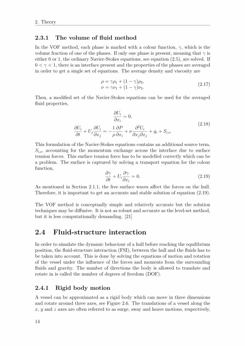
2.3.1 The volume of fluid method . . . . . . . . . . . . . . . . . . . 142.4 Fluid-structure interaction . . . . . . . . . . . . . . . . . . . . . . . . 14

2.4.1 Rigid body motion . . . . . . . . . . . . . . . . . . . . . . . . 142.4.2 Dynamic hull simulations . . . . . . . . . . . . . . . . . . . . 15

2.5 Non-dimensional coefficients . . . . . . . . . . . . . . . . . . . . . . . 16

ix

Contents

3 Numerical methods 173.1 The finite volume method . . . . . . . . . . . . . . . . . . . . . . . . 173.2 Spatial discretization schemes . . . . . . . . . . . . . . . . . . . . . . 18

3.2.1 VOF discretization schemes . . . . . . . . . . . . . . . . . . . 183.2.1.1 HRIC scheme . . . . . . . . . . . . . . . . . . . . . . 183.2.1.2 Compressive scheme . . . . . . . . . . . . . . . . . . 19

3.3 Temporal discretization schemes . . . . . . . . . . . . . . . . . . . . . 193.4 Pressure-velocity coupling . . . . . . . . . . . . . . . . . . . . . . . . 193.5 Dynamic meshing . . . . . . . . . . . . . . . . . . . . . . . . . . . . . 20

3.5.1 Diffusion-based smoothing . . . . . . . . . . . . . . . . . . . . 203.5.2 Overset method . . . . . . . . . . . . . . . . . . . . . . . . . . 21

3.6 Convergence criteria . . . . . . . . . . . . . . . . . . . . . . . . . . . 213.7 Grid dependence . . . . . . . . . . . . . . . . . . . . . . . . . . . . . 22

3.7.1 The grid convergence index procedure . . . . . . . . . . . . . . 23

4 CFD simulations 254.1 Computational domain definition . . . . . . . . . . . . . . . . . . . . 254.2 Mesh generation . . . . . . . . . . . . . . . . . . . . . . . . . . . . . . 264.3 Model definitions and properties . . . . . . . . . . . . . . . . . . . . . 27

4.3.1 Mathematical models . . . . . . . . . . . . . . . . . . . . . . . 274.3.1.1 Two-phase flow models . . . . . . . . . . . . . . . . . 284.3.1.2 Hull motion . . . . . . . . . . . . . . . . . . . . . . . 28

4.3.2 Numerical methods . . . . . . . . . . . . . . . . . . . . . . . . 284.4 Boundary conditions . . . . . . . . . . . . . . . . . . . . . . . . . . . 294.5 Solution . . . . . . . . . . . . . . . . . . . . . . . . . . . . . . . . . . 304.6 Post-processing . . . . . . . . . . . . . . . . . . . . . . . . . . . . . . 304.7 Simulated operating conditions . . . . . . . . . . . . . . . . . . . . . 30

4.7.1 Athena hull . . . . . . . . . . . . . . . . . . . . . . . . . . . . 304.7.2 Swede Ship hull . . . . . . . . . . . . . . . . . . . . . . . . . . 31

5 Results and discussion 355.1 Athena hull . . . . . . . . . . . . . . . . . . . . . . . . . . . . . . . . 35

5.1.1 Grid dependence study . . . . . . . . . . . . . . . . . . . . . . 355.1.2 Calculated properties . . . . . . . . . . . . . . . . . . . . . . . 36

5.2 Swede Ship hull, fixed sinkage and trim . . . . . . . . . . . . . . . . . 385.2.1 Grid dependence study . . . . . . . . . . . . . . . . . . . . . . 385.2.2 Volume fraction of air at the hull . . . . . . . . . . . . . . . . 395.2.3 Pressure coefficient . . . . . . . . . . . . . . . . . . . . . . . . 405.2.4 Skin friction coefficient . . . . . . . . . . . . . . . . . . . . . . 415.2.5 Dimensionless wall distance . . . . . . . . . . . . . . . . . . . 425.2.6 Free surface wave pattern . . . . . . . . . . . . . . . . . . . . 435.2.7 Calculated properties . . . . . . . . . . . . . . . . . . . . . . . 44

5.3 Swede Ship hull, free sinkage and trim . . . . . . . . . . . . . . . . . 455.3.1 Grid dependence study . . . . . . . . . . . . . . . . . . . . . . 455.3.2 Centre of gravity sensitivity analysis . . . . . . . . . . . . . . 475.3.3 Calculated properties . . . . . . . . . . . . . . . . . . . . . . . 475.3.4 Free surface wave pattern . . . . . . . . . . . . . . . . . . . . 51

x

Contents

5.3.5 FLUENT simulations of free sinkage and trim . . . . . . . . . 52

6 Conclusion 53

7 Future work 55

References 57

A Data analysis I

B Athena hull data III

C Swede Ship hull data V

D Grid dependence studies VII

xi

Contents

xii

List of figures

1.1 Work flow of the CFD simulations. . . . . . . . . . . . . . . . . . . . 42.1 Characteristic parts of a hull. . . . . . . . . . . . . . . . . . . . . . . 52.2 Characteristic hull measurements. . . . . . . . . . . . . . . . . . . . . 62.3 Kelvin wake pattern behind a moving object. . . . . . . . . . . . . . . 72.4 A planing hull in front view. . . . . . . . . . . . . . . . . . . . . . . . 82.5 Schematic illustration of a boundary layer at a flat plate. . . . . . . . 122.6 Coordinate system showing the 6 degrees of freedom of a rigid body. . 152.7 Iterative procedure of a hull simulation used to describe the fluid-

structure interaction. . . . . . . . . . . . . . . . . . . . . . . . . . . . 163.1 Schematic illustrations of dynamic meshes around a tilted square. . . 204.1 Dimensions of the computational domain. . . . . . . . . . . . . . . . 254.2 Schematic illustrations of the FLUENT mesh structure. . . . . . . . . 264.3 Schematic illustrations of the STAR-CCM+ mesh structure. . . . . . 274.4 Boundaries of the computational domain. . . . . . . . . . . . . . . . . 294.5 Sketch of the Athena hull showing the two different centres of gravity,

CG1 and CG2, used in the simulations. . . . . . . . . . . . . . . . . . 314.6 Sketch of the Swede Ship hull showing the centre of gravity (CG) and

the centre of buoyancy (CB) at zero speed. . . . . . . . . . . . . . . . 325.1 Convergence of the total resistance coefficient with grid refinement for

the free sinkage and trim simulations of the Athena hull performedin STAR-CCM+ at Fn = 0.545. . . . . . . . . . . . . . . . . . . . . 36

5.2 Volume fraction of air at the symmetry plane of the Athena hull atFn = 0.545. . . . . . . . . . . . . . . . . . . . . . . . . . . . . . . . . 37

5.3 Cross sections at different y-coordinates used in the illustrations ofthe results. . . . . . . . . . . . . . . . . . . . . . . . . . . . . . . . . . 38

5.4 Convergence of the total resistance coefficient with grid refinementfor the fixed sinkage and trim simulations of the Swede Ship hullperformed in FLUENT at Fn = 1.68. . . . . . . . . . . . . . . . . . . 39

5.5 Contour plots of the volume fraction of air on the hull for the fixedsinkage and trim simulations at Fn = 1.68. . . . . . . . . . . . . . . . 39

5.6 Contour plots of the pressure coefficient on the hull for the fixedsinkage and trim simulations at Fn = 1.68. . . . . . . . . . . . . . . . 40

5.7 Longitudinal cross sections of the pressure coefficient on the hull forthe fixed sinkage and trim simulations at Fn = 1.68. . . . . . . . . . 40

5.8 Transverse cross sections of the pressure coefficient on the hull for thefixed sinkage and trim simulations at Fn = 1.68. . . . . . . . . . . . . 41

xiii

List of figures

5.9 Contour plots of the skin friction coefficient on the hull for the fixedsinkage and trim simulations at Fn = 1.68. . . . . . . . . . . . . . . . 41

5.10 Longitudinal cross sections of the skin friction coefficient on the hullfor the fixed sinkage and trim simulations at Fn = 1.68. . . . . . . . 42

5.11 Contour plots of the dimensionless wall distance on the hull for thefixed sinkage and trim simulations at Fn = 1.68. . . . . . . . . . . . . 42

5.12 Contour plots of the dimensionless free surface height for the fixedsinkage and trim simulations at Fn = 1.68. . . . . . . . . . . . . . . . 43

5.13 Cross sections of the dimensionless free surface height at Fn = 1.68. . 445.14 Convergence of the total resistance coefficient with grid refinement for

the free sinkage and trim simulations of the Swede Ship hull performedin STAR-CCM+ at Fn = 1.68. . . . . . . . . . . . . . . . . . . . . . 45

5.15 Convergence of the sinkage with grid refinement for the free sinkageand trim simulations of the Swede Ship hull performed in STAR-CCM+ at Fn = 1.68. . . . . . . . . . . . . . . . . . . . . . . . . . . . 46

5.16 Convergence of the trim angle with grid refinement for the free sinkageand trim simulations of the Swede Ship hull performed in STAR-CCM+ at Fn = 1.68. . . . . . . . . . . . . . . . . . . . . . . . . . . . 46

5.17 Computational and experimental results for the Froude number de-pendency of the total resistance for the Swede Ship hull with freesinkage and trim. . . . . . . . . . . . . . . . . . . . . . . . . . . . . . 48

5.18 Computational and experimental results for the Froude number de-pendency of the sinkage for the Swede Ship hull with free sinkage andtrim. . . . . . . . . . . . . . . . . . . . . . . . . . . . . . . . . . . . . 48

5.19 Computational and experimental results for the Froude number de-pendency of the trim angle for the Swede Ship hull with free sinkageand trim. . . . . . . . . . . . . . . . . . . . . . . . . . . . . . . . . . 49

5.20 Computational and experimental results for the Froude number de-pendency of the wetted area for the Swede Ship hull with free sinkageand trim. . . . . . . . . . . . . . . . . . . . . . . . . . . . . . . . . . 50

5.21 Computational and experimental results for the Froude number de-pendency of the wetted length for the Swede Ship hull with free sink-age and trim. . . . . . . . . . . . . . . . . . . . . . . . . . . . . . . . 50

5.22 Contour plots of the dimensionless free surface height for the freesinkage and trim simulations obtained in STAR-CCM+ at Fn =0.447, Fn = 0.894 and Fn = 1.68. . . . . . . . . . . . . . . . . . . . . 51

5.23 Dimensionless free surface height around the free hull at Fn = 1.68showing the unphysical dislocation of the free surface when the hullmoves downwards and upwards. . . . . . . . . . . . . . . . . . . . . . 52

xiv

List of tables

4.1 Hull dimensions of R/V Athena. . . . . . . . . . . . . . . . . . . . . . 314.2 Fluid properties used in the simulations of the Athena hull. . . . . . . 314.3 Properties and dimensions of the Swede Ship hull at a water density

of 1025.87 kg/m3 and a shell plating thickness of 8.00mm. . . . . . . 324.4 Fluid properties used in the simulations of the Swede Ship hull. . . . 324.5 Simulated cases for the Swede Ship hull with fixed sinkage and trim. . 334.6 Simulated cases for the Swede Ship hull with free sinkage and trim. . 335.1 Experimental and calculated properties of the Athena hull with free

sinkage and trim at Fn = 0.545. . . . . . . . . . . . . . . . . . . . . . 365.2 Calculated properties of the Swede Ship hull with fixed sinkage at

LPP/2 and trim angle of 0.685m and 3.19, respectively, at Fn = 1.68. 445.3 Calculated properties of the Swede Ship hull with free sinkage and

trim at Fn = 1.68. . . . . . . . . . . . . . . . . . . . . . . . . . . . . 47B.1 Hull dimensions of R/V Athena. . . . . . . . . . . . . . . . . . . . . . IIIB.2 Fluid properties used in the simulations for the Athena hull. . . . . . IIIC.1 Dimensions of the Swede Ship hull. . . . . . . . . . . . . . . . . . . . VC.2 Properties of the Swede Ship hull at a water density of 1025.87 kg/m3

and a shell plating thickness of 8.00mm. . . . . . . . . . . . . . . . . VC.3 Fluid properties used in the simulations of the Swede Ship hull. . . . VID.1 Number of cells in the meshes used in the grid dependence study of

the Athena hull with free sinkage and trim at Fn = 0.545. . . . . . . VIID.2 Number of cells in the meshes used in the grid dependence study of

the Swede Ship hull with fixed sinkage and trim at Fn = 1.68. . . . . VIID.3 Number of cells in the meshes used in the grid dependence study of

the Swede Ship hull with free sinkage and trim at Fn = 1.68. . . . . . VII

xv

List of tables

xvi

Acronyms

In the following table, expansions of the acronyms used in the report are presented.

Acronym Expansion

AP Aft perpendicular

CAD Computer-aided design

CFD Computational fluid dynamics

DNS Direct numerical simulation

DOF Degrees of freedom

EFD Experimental fluid dynamics

FP Forward perpendicular

FSI Fluid-structure interaction

FVM Finite volume method

GCI Grid convergence index

HRIC High resolution interface capturing scheme

PDE Partial differential equation

RANS Reynolds averaged Navier-Stokes

SIMPLE Semi-implicit method for pressure linked equations

SST Shear stress transport

UDF User defined function

VOF Volume of fluid

xvii

Acronyms

xviii

Nomenclature

In the following tables, the nomenclature used in the report is explained. For theGreek and Roman symbols, the physical dimensions are expressed in the base di-mensions mass (M), length (L) and time (T). When a variable is not connected toa certain physical quantity, the dimension field is marked with a star (?).

AccentsAccent Description

Time average−→ Vector

Greek symbolsSymbol Description Dimensions

α Diffusion parameter 1

δij Kronecker delta 1

δRE Discretization error estimation ?

ε Dissipation of turbulent kinetic energy L2T−3

Γ Diffusivity L2T−1

γ Colour function used in the VOF method 1

Γm Mesh diffusivity L2T−1

∇ Volume displacement L3

ν Kinematic viscosity L2T−1

νt Turbulent viscosity L2T−1

Ω Angular velocity T−1

ω Specific dissipation of turbulent kineticenergy

T−1

φ General flow variable ?

φnb Value of general flow variable in neigh-bouring cells

?

xix

Nomenclature

φP Value of general flow variable in presentcell

?

ρ Density ML−3

σ Surface tension MT−2

τ Torque ML2T−2

τw Wall shear stress ML−1T−2

θ Trim angle 1

Roman symbolsSymbol Description Dimensions

anb Discretization coefficients associated toneighbouring cells

?

aP Discretization coefficient associated topresent cell

?

AW Wetted area L2

Cε1, Cε2Cµ, σk, σε

Constants of the k-ε turbulence model 1

Cω1, Cω2β∗, σωk , σω

Constants of the k-ω turbulence model 1

d Normalized boundary distance 1

ED Discretization uncertainty ?

EI Iterative uncertainty ?

EN Numerical uncertainty ?

F Force MLT−2

FS Factor of safety used in GCI 1

g Gravitational acceleration LT−2

hi Characteristic cell length of grid i 1

k Turbulent kinetic energy L2T−2

L Length L

LOA Length overall L

LPP Length between perpendiculars L

LW Wetted length L

M Moments of inertia (tensor) ML2

m Mass M

xx

Nomenclature

N Number of cells 1

P Pressure ML−1T−2

p Fluctuating pressure ML−1T−2

P∞ Pressure of free stream ML−1T−2

Pk Production of turbulent kinetic energy L2T−3

q Richardson extrapolation constant ?

r Richardson extrapolation observed orderof accuracy

1

Rnorm Residual normalization value ?

Rφ Residual of flow variable φ ?

Rφ,s Residual of flow variable φ, globallyscaled

?

Rpres Present value of residual ?

rr Grid refinement ratio 1

Rrms Root mean square residual ?

Rtot Total resistance MLT−2

S Source term in transport equation ?

s Sinkage L

S0 Extrapolated solution for an infinite griddensity

?

Si Solution on grid i ?

SP Variable depending part of source term ?

SU Constant part of source term ?

T Draught L

t Time T

U Velocity LT−1

u Fluctuating velocity LT−1

Uhull Hull velocity LT−1

u∗ Friction velocity LT−1

xi Spatial coordinate in dimension i L

y+ Dimensionless wall distance 1

xxi

Nomenclature

Dimensionless numbersSymbol Name Definition

Cf Skin friction coefficient Cf = τw12ρU

2hull

CP Pressure coefficient CP = P − P∞12ρU

2hull

CT Total resistance coefficient CT = Rtot12ρU

2hullAW0

Fn Froude number Fn = Uhull√Lg

Rn Reynolds number Rn = UhullL

ν

Wn Weber number Wn = ρU2hullL

σ

SubscriptsSubscript Description

AP Aft perpendicular

FP Forward perpendicular

xxii

1Introduction

Hull design is a field of engineering that has been developed for hundreds of years.Today, the main focus is to meet the contract speed requirements with minimum fuelconsumption. It is important to make an accurate prediction of the hull resistanceto be able to choose an appropriate engine power of the propulsion unit. It is alsoof interest to investigate the running attitude of the hull to get desirable seakeepingproperties.

Traditionally, the hull resistance and running attitude have been determined byperforming experiments on down scaled model hulls in towing tanks. These experi-ments have proved to predict the behaviour of the full scale hull very well, but themethod is time consuming, expensive and only applicable to the tested model. Amore universal method for hull performance predictions is to use computational fluiddynamics (CFD) which is a branch of computer simulations where the behaviour ofa system involving fluid flow is analysed using numerical methods.

There are well established methods for CFD simulations of displacement hulls andthe results predict the behaviour of the hull with high accuracy. Resistance pre-dictions of planing hulls are more difficult, and a lot of today’s research is focusedon improving CFD methods for planing hulls. In contrast to displacement hulls,which are supported by hydrostatic forces acting on the hull, planing hulls utilizehydrodynamic forces from the water to reduce the resistance and thereby be able toreach high speeds with relatively low fuel consumption.

This study is done in cooperation with Swede Ship Marine AB which is a companythat designs and manufactures high speed planing vessels such as rescue vessels,pilot boats, coast guard vessels and navy vessels. If Swede Ship could make use ofCFD in their hull development, they could improve their vessel design process andreduce the production time and cost.

1.1 BackgroundHull development has traditionally relied on model scale experiments in towingtanks. Instead of doing these experiments, empirical models based on regressionanalysis of experimental data have been developed to predict the behaviour basedon the characteristics of the hull shape. Two widely used empirical models are thatof Holtrop and Mennen [1], used for displacement hulls, and that of Savitsky [2],

1

1. Introduction

used for planing hulls. The main drawback with these empirical models is that theyare restricted to simple hull shapes which are similar to the hulls used to developthe models.

During the last decades, several numerical studies on planing hulls have been per-formed. Brizzolara and Serra [3] compared CFD simulations of planing hulls withthe Savitsky method. The flow was modelled with the RANS equations and thestandard k-ε model was used to model the turbulence. The VOF method was usedto resolve the free surface. It was found that the hull resistance from the CFDsimulations differed in average 10% from the experimental results. This was lowerthan the error of the Savitsky method, and the study showed the potential of CFDsimulations.

In order to find the running attitude of a vessel, its motion must be included in thesimulation. For this purpose, methods for coupling the fluid flow and body motionshave been developed. Azcueta [4] implemented a method in 2001 where the inter-action between the hull and the fluid was modelled. The turbulence was modelledwith the RANS equations and the standard k-ε model, and the free surface was cap-tured with a VOF method. The method was validated for a Series 60 Hull, which isa well-known displacement hull used for simulation benchmarking, and the resultswere compared with experimental data. The total resistance was underpredicted by5.9% and the sinkage and trim were 8.2% and 6.0% lower than the experimentalresults respectively.

Recent studies show that CFD simulations of displacement hulls have been madewith a precision that start to approach that of towing tank tests. At the Workshopon Numerical Ship Hydrodynamics in Gothenburg 2010 [5, pp. 1–16], 33 partici-pating groups performed simulations of three large displacement ships. The resultsfrom all simulations show that the mean error of the resistance predictions, in com-parison to towing tank experiments, was only 0.1% with a standard deviation of2.1%. The sinkage and trim predictions were less accurate, for the higher speedsthe mean errors were around 4%.

CFD simulation of planing hulls is more challenging in comparison to displacementhulls, and in general the accuracy of the predictions is lower. The viscous forces fromthe flow around a planing hull are strongly dependent on the wet surface of the hull,which in turn depends on the position in the water. It is therefore crucial to predicthow a planing hull behaves in water before adequate resistance estimations can bemade. [6] Also, in the higher speed range, nonlinear effects such as breaking wavesand water sprays become more important. However, as the computer power steadilyincreases and better models are developed, the results from numerical simulationsof planing hulls are continuously improved. [7] The results from recent studies [8,9] have shown that CFD simulations of planing hulls can yield results that deviatefrom experimental data by less than 10%.

2

1. Introduction

1.2 Purpose and objectivesThe purpose of this study is to evaluate how accurate CFD is using commerciallyavailable software, and if these can fully or partly replace towing tank tests in planinghull design. This is done by calculating the resistance, sinkage and trim angle ofa high speed planing hull, whereupon the results are compared with experimentaldata. In this study, the simulations have been performed using two of the mostcommon general purpose CFD software, ANSYS FLUENT, developed by ANSYS,Inc., and STAR-CCM+, developed by CD-adapco.

1.3 DemarcationsThe focus of this study is on the stationary behaviour of planing hulls moving incalm water at a constant speed. The vessel is limited to heave and pitch motions.An economical evaluation of the method is not included.

1.4 Research questionsThe following questions are addressed in this report.

• How accurately can the resistance and running attitude of a planing hull bepredicted using CFD simulations?

• Do the CFD simulations yield any additional information that is not obtainedfrom model testing?

• Are there any differences in the results obtained from FLUENT andSTAR-CCM+?

1.5 MethodA flow chart outlining the methodology of the CFD simulations is presented inFigure 1.1. The strategies differ in FLUENT and STAR-CCM+, and are basedon guidelines for hull simulations provided by each software developer. The workstarts with defining the computational domain required to perform the analysis, andthen the computational meshes are generated. When appropriate models have beenchosen in the model definitions step and the boundary conditions have been set, thesolution can be initiated. The computational domain is the same for FLUENT andSTAR-CCM+, while the mesh generation, model definitions, boundary conditionsand solution steps are done separately. When the results are obtained, they areanalysed in the post processing step. These steps are made in an iterative processwhere the results are evaluated and further simulations are performed.

3

1. Introduction

Start

Computationaldomain definition

Mesh generation

Model definitions

Boundary conditions

Solution

Post processing

End

FLUENT STAR-CCM+

Figure 1.1: Work flow of the CFD simulations.

1.6 Report structureThe report is organized in the following way. In Chapter 2, the theory behindplaning hulls and the different types of resistance forces that are acting on the hullare explained. In the same chapter the mathematical models governing the fluids,the fluid interface and the vessel motion are presented. The numerical methods usedfor treating these equations are described in Chapter 3. Chapter 4 describes how theCFD simulations were performed and in Chapter 5, the results are presented anddiscussed. Finally, the conclusions are presented in Chapter 6 and recommendationsfor future work are given in Chapter 7.

4

2Theory

This chapter aims to provide the theoretical basis for understanding the remainderof the report. It starts with a section introducing the basics of naval architecturerelated to planing hulls, and continues with describing the mathematical modelsused in the simulation of a hull in motion.

2.1 Planing hull theoryIn Figure 2.1, some of the characteristic parts of a planing hull are highlighted. Thebow and stern are the front and back of the vessel and the transom is the verticalsurface located at the stern. The spray rails and lifting rails are used to guide thewater flow along the hull in order to obtain the desired behaviour of the vessel whenmoving through the water.

Lifting rail

Spray rail

Transom

BowStern

Figure 2.1: Characteristic parts of a hull.

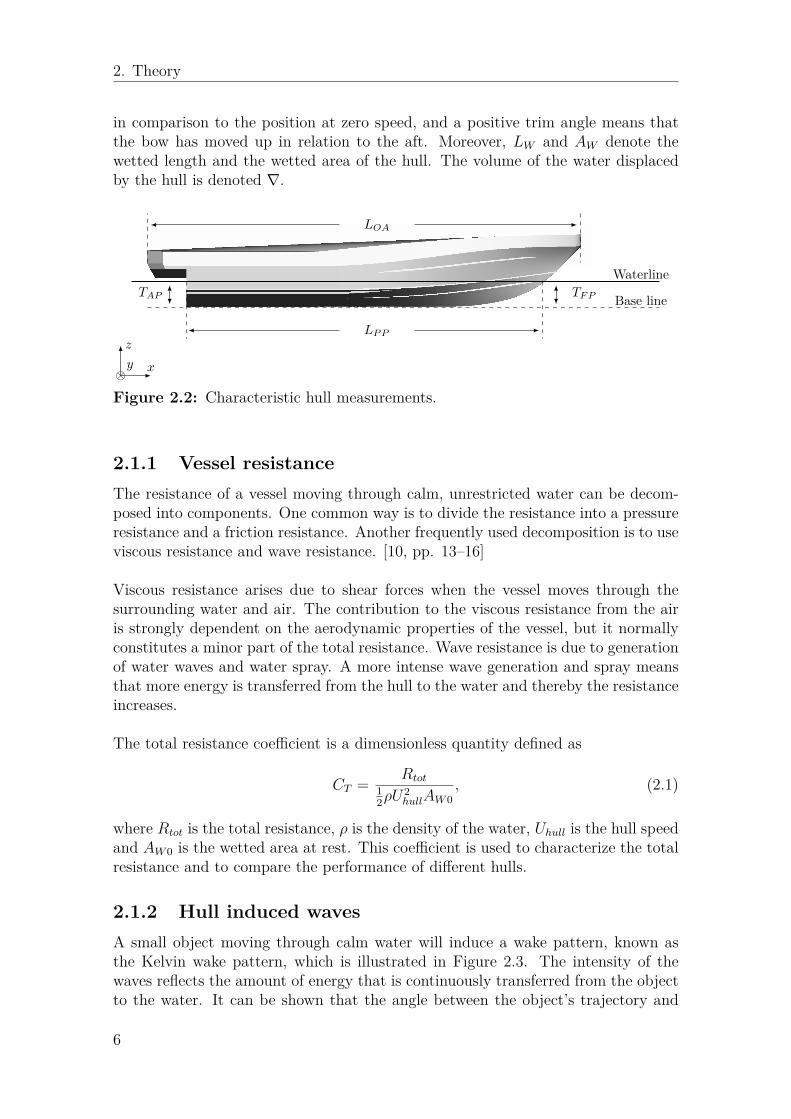
In naval architecture, the properties of a hull can be characterized by certain mea-surements shown in Figure 2.2. The measurements used are the overall length, LOA,length between perpendiculars, LPP , and the draughts at the forward and aft per-pendiculars, TFP and TAP . The aft perpendicular (AP) is a point on the verticaltransom, and the forward perpendicular (FP) is the point where the waterline in-tersects the keel in the front.

When the vessel is in motion, its position can be related to that of zero speed bymeasuring the change in vertical position of these perpendiculars. This change isknown as the sinkage, s, which is defined as positive if the elevation of the perpen-dicular has increased. The trim angle, θ, is the angle of rotation around the y-axis

5

2. Theory

in comparison to the position at zero speed, and a positive trim angle means thatthe bow has moved up in relation to the aft. Moreover, LW and AW denote thewetted length and the wetted area of the hull. The volume of the water displacedby the hull is denoted ∇.

Waterline

LP P

LOA

Base lineTF PTAP

x

z

⊗y

Figure 2.2: Characteristic hull measurements.

2.1.1 Vessel resistanceThe resistance of a vessel moving through calm, unrestricted water can be decom-posed into components. One common way is to divide the resistance into a pressureresistance and a friction resistance. Another frequently used decomposition is to useviscous resistance and wave resistance. [10, pp. 13–16]

Viscous resistance arises due to shear forces when the vessel moves through thesurrounding water and air. The contribution to the viscous resistance from the airis strongly dependent on the aerodynamic properties of the vessel, but it normallyconstitutes a minor part of the total resistance. Wave resistance is due to generationof water waves and water spray. A more intense wave generation and spray meansthat more energy is transferred from the hull to the water and thereby the resistanceincreases.

The total resistance coefficient is a dimensionless quantity defined as

CT = Rtot12ρU

2hullAW0

, (2.1)

where Rtot is the total resistance, ρ is the density of the water, Uhull is the hull speedand AW0 is the wetted area at rest. This coefficient is used to characterize the totalresistance and to compare the performance of different hulls.

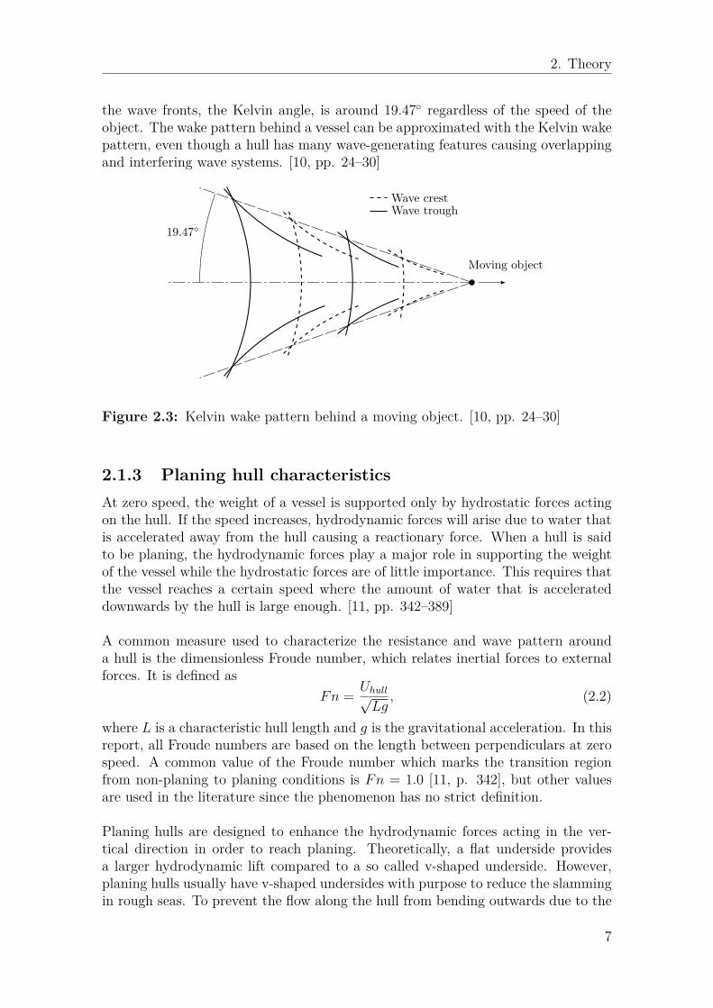
2.1.2 Hull induced wavesA small object moving through calm water will induce a wake pattern, known asthe Kelvin wake pattern, which is illustrated in Figure 2.3. The intensity of thewaves reflects the amount of energy that is continuously transferred from the objectto the water. It can be shown that the angle between the object’s trajectory and

6

2. Theory

the wave fronts, the Kelvin angle, is around 19.47 regardless of the speed of theobject. The wake pattern behind a vessel can be approximated with the Kelvin wakepattern, even though a hull has many wave-generating features causing overlappingand interfering wave systems. [10, pp. 24–30]

Moving object

19.47

Wave crestWave trough

Figure 2.3: Kelvin wake pattern behind a moving object. [10, pp. 24–30]

2.1.3 Planing hull characteristicsAt zero speed, the weight of a vessel is supported only by hydrostatic forces actingon the hull. If the speed increases, hydrodynamic forces will arise due to water thatis accelerated away from the hull causing a reactionary force. When a hull is saidto be planing, the hydrodynamic forces play a major role in supporting the weightof the vessel while the hydrostatic forces are of little importance. This requires thatthe vessel reaches a certain speed where the amount of water that is accelerateddownwards by the hull is large enough. [11, pp. 342–389]

A common measure used to characterize the resistance and wave pattern arounda hull is the dimensionless Froude number, which relates inertial forces to externalforces. It is defined as

Fn = Uhull√Lg, (2.2)

where L is a characteristic hull length and g is the gravitational acceleration. In thisreport, all Froude numbers are based on the length between perpendiculars at zerospeed. A common value of the Froude number which marks the transition regionfrom non-planing to planing conditions is Fn = 1.0 [11, p. 342], but other valuesare used in the literature since the phenomenon has no strict definition.

Planing hulls are designed to enhance the hydrodynamic forces acting in the ver-tical direction in order to reach planing. Theoretically, a flat underside providesa larger hydrodynamic lift compared to a so called v-shaped underside. However,planing hulls usually have v-shaped undersides with purpose to reduce the slammingin rough seas. To prevent the flow along the hull from bending outwards due to the

7

2. Theory

v-shape, lifting rails are used to guide the flow backwards and thereby increase thehydrodynamic pressure under the hull. Spray rails can be used on the hull sidesto increase the lift force by bending the water spray downwards. [10, pp. 175–181]Furthermore, it is important that the water separates from the hull at the transomin order to avoid sub-atmospheric pressures that could lead to instabilities. [12] Thiscan be achieved by using a sharp edge at the transom where the water is supposedto detach from the hull.

The same hull as in Figure 2.1 and 2.2 is shown in a front view in Figure 2.4. Itcan be seen that it has a v-shaped underside and is equipped with lifting rails andspray rails which are characteristic features of a planing hull.

y

z

x

Figure 2.4: A planing hull in front view.

2.1.4 Towing tank testsWhen designing a vessel, the properties of the hull are traditionally tested at anearly stage by constructing a smaller model which can be used in experiments.These experiments can be performed in open water, but to reduce the sources oferrors, they are often carried out in large tanks known as towing tanks. In a towingtank, the hull is towed through the water while measurements are conducted.

2.1.4.1 Model test scaling

When towing tank tests have been carried out on a model, the results must be scaledproperly in order to apply to a hull in full scale. To achieve adequate scaling results,the model and the full scale hull must be geometrically similar and the relevantdimensionless numbers should be preserved. For a planing hull, the dimensionlessnumbers characterising the physics of the flow are the Froude number, the Reynoldsnumber and the Weber number. The Froude number, as defined in equation (2.2),describes the effect of gravity on the water surface. The Reynolds number relatesinertial forces to viscous forces, and is defined as

Rn = UhullL

ν, (2.3)

8

2. Theory

where ν is the kinematic viscosity. The Weber number relates inertial forces toforces due to surface tension, and is defined as

Wn = ρU2hullL

σ, (2.4)

where σ is the surface tension.

A dilemma related to scaling is the inability to satisfy the conservation of thesethree dimensionless numbers simultaneously. As can be seen from the definitionsof the three dimensionless numbers, a model scale hull with shorter length musthave a lower speed to preserve the Froude number but a higher speed to preservethe Reynolds and Weber numbers. The established solution to this problem is touse the same Froude number in the model tests and to account for the differentReynolds numbers in the scaling process. The difference in Weber numbers betweenmodel scale and full scale causes errors in the predictions of water spray, foamingand wave pattern, but it has been concluded that this has little influence on theresistance prediction of the full scale hull. [10, pp. 10–13]

2.2 TurbulenceWhen a hull is moving through water at high speed, the flow around the hull isturbulent. In this section, the governing equations of turbulent flows are presentedand turbulence modelling is explained.

2.2.1 Turbulent flowTurbulence has no physical definition, but it is characterized as a three-dimensional,irregular flow where turbulent kinetic energy is dissipated from the largest to thesmallest turbulent scales. On the smallest turbulent scales, known as the Kol-mogorov scales, the energy is dissipated into heat due to viscous forces. Sinceturbulence is a dissipative phenomenon, energy must be continuously supplied inorder to maintain a turbulent flow.

The motion of a viscous fluid is governed by the Navier-Stokes equations, whichare valid both for turbulent and laminar flow. For an incompressible, Newtonianfluid in three dimensions under the influence of an external gravitational field, theNavier-Stokes equations read

∂Ui∂xi

= 0,

∂Ui∂t

+ Uj∂Ui∂xj

= −1ρ

∂P

∂xi+ ν

∂2Ui∂xj∂xj

+ gi.

(2.5)

Here, the equations are formulated using tensor notation. The indices i and j inthe Navier-Stokes equations run over the spatial coordinates x, y and z. In theseequations, Ui is the velocity in dimension i, xi is the spatial coordinate in dimension

9

2. Theory

i, t is time, ρ is the density, P is the pressure, ν is the kinematic viscosity and gi isthe gravitational acceleration.

Analytical solutions to the Navier-Stokes equations only exist for a limited num-ber of simple cases such as laminar flow between flat plates. For turbulent flowsin engineering applications, analytical solutions do not exist and the Navier-Stokesequations must be treated numerically. If they are solved using direct numericalsimulation (DNS), the velocity field of the flow is obtained. However, since tur-bulence occurs on a wide range of time and length scales, DNS requires very hightemporal and spatial resolutions to capture all the details of the flow. Thus, DNSis very computationally expensive and time consuming which limits the method tospecial applications such as academic research or simulation of simple flows.

2.2.2 Turbulence modellingThe most common way of treating turbulence is to use turbulence models in whichthe turbulent features of the flow are not resolved in time. By performing Reynoldsdecomposition, the instantaneous velocity and pressure can be decomposed as

Ui = Ui + ui,P = P + p,

(2.6)

where Ui and P denote the time averaged quantities while ui and p are the fluc-tuating components of the velocities and the pressure. By inserting the Reynoldsdecomposition into the Navier-Stokes equations given in equation 2.5, the Reynoldsaveraged Navier-Stokes (RANS) equations are obtained. These are written as

∂Ui∂xi

= 0,

∂Ui∂t

+ Uj∂Ui∂xj

= −1ρ

∂P

∂xi+ ν

∂2Ui∂xj∂xj

− ∂uiuj∂xj

+ gi.

(2.7)

It can be noted that the RANS equations are very similar to the Navier-Stokesequations except for the additional term including uiuj, referred to as the Reynoldsstress tensor. If the Reynolds stress term is modelled, the RANS equations describethe time-averaged flow quantities which requires substantially less computationalresources in comparison to DNS.

A common approach for modelling the Reynolds stress tensor of the RANS equa-tions is to use the Boussinesq approximation. In this assumption, the Reynoldsstress tensor is modelled as a diffusion term by introducing a turbulent viscosity, νt,according to

− uiuj = νt

(∂Ui∂xj

+ ∂Uj∂xi

)− 2

3kδij. (2.8)

In this equation, δij is the Kronecker delta which assumes a value of 1 if i = j and0 otherwise, and k is the turbulent kinetic energy defined as

k = 12uiui. (2.9)

10

2. Theory

By using a model to describe how the turbulent viscosity depends on the flow, theRANS equations can be solved. The so called two-equation turbulence models, suchas the k-ε model and the k-ω model, use two additional transport equations todescribe the turbulent viscosity. They are referred to as complete models since theyallow the turbulent velocity and length scales to be described independently. [13]

2.2.2.1 The standard k-ε model

In the standard k-ε model, the transport equations for the turbulent kinetic en-ergy and its dissipation, ε, are used to obtain the turbulent viscosity. It has beendescribed by Launder et al. [14], and the model equations are

∂k

∂t+ ∂

∂xi

(kUi

)= ∂

∂xj

[(ν + νt

σk

)∂k

∂xj

]+ Pk − ε,

∂ε

∂t+ ∂

∂xi

(εUi

)= ∂

∂xj

[(ν + νt

σε

)∂ε

∂xj

]+ ε

k(Cε1Pk − Cε2ε) ,

νt = Cµk2

ε,

(2.10)

where σk, σε, Cε1, Cε2 and Cµ are model constants and Pk is the production ofturbulent kinetic energy. The latter is defined as

Pk = −uiuj∂Ui∂xj

(2.11)

and is modelled using the Boussinesq approximation.

The standard k-ε model is robust and gives good predictions for free flows with smallpressure gradients. It is based on the assumption that the flow is fully turbulentwhich limits its applicability to high Reynolds number flows. [15] Over time, it hasbeen observed that the standard k-ε model cannot be used to describe the wakebehind a moving hull in a satisfactory manner. [10, p. 135]

2.2.2.2 The k-ω model

In the k-ω model described by Wilcox [15], the transport equations for the turbulentkinetic energy and its specific dissipation, ω, are used in a similar way as for thestandard k-ε model. The specific dissipation is related to the dissipation accordingto

ω ∝ ε

k. (2.12)

The model equations for k and ω are∂k

∂t+ ∂

∂xi

(kUi

)= ∂

∂xj

[(ν + νt

σωk

)∂k

∂xj

]+ Pk − β∗kω,

∂ω

∂t+ ∂

∂xi

(ωUi

)= ∂

∂xj

[(ν + νt

σω

)∂ω

∂xj

]+ ω

k(Cω1Pk − Cω2kω) ,

νt = k

ω,

(2.13)

11

2. Theory

where β∗, σωk , σω, Cω1 and Cω2 are model constants.

The k-ω model has the advantage that it is also valid close to walls and in regionsof low turbulence. [16, pp. 121–122] Thus, it is valid also in the low turbulentReynolds number region close to walls, meaning that the transport equations canbe used in the whole flow domain. A drawback with the k-ω model is that theresults are sensitive to the choice of boundary conditions and initial conditions.

2.2.2.3 The SST k-ω model

In order to make use of the collective advantages of the k-ε and k-ω models, Menter[17] developed the shear stress transport (SST) model by combining the two modelsinto one using blending functions. In this hybrid model, the k-ω model is used in theboundary layer while the k-ε model, formulated on k-ω form, is used in the free flow.

The SST k-ω model has shown good performance for many types of complex flows,such as in flows with adverse pressure gradients and separating flows, where thek-ε or the k-ω models have given results that differ significantly from experimentaldata. It has been recognized for its good overall performance [18] and it is the mostcommonly used turbulence model for simulations of ship hydrodynamics. [19, p. 7]

2.2.3 Boundary layersWhen a fluid flows along a surface, shear stresses give rise to a boundary layer inthe vicinity of the surface. The structure of a boundary layer near the edge of aflat plate is illustrated in Figure 2.5, where the incident flow has a uniform velocityprofile with velocity U0. When the flow reaches the plate, a laminar boundary layerstarts to grow at the surface. After some distance, the boundary layer goes intoa transition region after which a turbulent boundary layer is developed. The flowin the inner part of the turbulent boundary layer is laminar, and the turbulenceincreases further away from the wall. [20, pp. 464–475]

U0 U(y)

Laminarboundary layer

Transitionregion

Turbulentboundary layer

Viscous sub-layerBuffer sub-layer

Fully turbulentsub-layer

y

Figure 2.5: Schematic illustration of a boundary layer at a flat plate. [20, pp.464–475]

12

2. Theory

To characterize the flow near a wall, a dimensionless wall distance is often intro-duced. It is defined as

y+ = u∗y

ν, (2.14)

where y is the distance to the wall and u∗ is a friction velocity. The friction velocityis defined as

u∗ =√τwρ, (2.15)

where τw is the wall shear stress,

τw = ρν∂U

∂y

∣∣∣∣∣y=0

. (2.16)

In the boundary layer, the gradients of the flow variables in the wall-normal direc-tion are generally very large in comparison to those of the free flow. This impliesthat a high spatial resolution is required by the solution method in order to capturethe effects near the wall. A common alternative method used to circumvent therequirement of a high spatial resolution is to use wall functions, which are empiricalmodels used to estimate the flow variables near walls. Wall functions can also beapplied when the turbulence model used in a simulation is not valid close to thewall, which for example is the case for the standard k-ε model. [16, pp. 128–140]Although wall functions are undesired in computational ship hydrodynamics due todeviations for some types of flow, they are often used for numerical reasons. [10, pp.152–154]

Standard wall functions are based on the assumption that the boundary layer can bedescribed as a flat plate boundary layer. This means that the time-averaged velocitycan be expressed as a function of the dimensionless wall distance. In the viscoussub-layer, it can be shown that the velocity parallel to the wall is proportional toy+. In the fully turbulent sub-layer, the velocity follows the logarithmic law ofthe wall, meaning that the velocity is proportional to the natural logarithm of y+.Between these sub-layers, in the buffer sub-layer, there is a transition from linear tologarithmic y+ dependence. In order for a wall function to work properly, it shouldbe used all the way to the fully turbulent layer which corresponds to a value of y+

above 30. The wall functions also estimate the turbulence quantities near the walls.[16, pp. 128–140]

2.3 Free water surfaceIn order to simulate a hull moving in water, models are needed to resolve the interfacebetween the water and air. There are different two-phase models available that eithertracks the surface directly or tracks the different phases and then reconstructs theinterface. One example is the level-set method, where all molecules of one phaseare marked and then tracked in the fluid flow. The most frequently used method tocapture the free surface in ship hydrodynamics is the volume of fluid (VOF) method[5, pp. 5–9]. In the VOF method, the different phases are tracked. [10, pp. 151–152]

13

2. Theory

2.3.1 The volume of fluid methodIn the VOF method, each phase is marked with a colour function, γ, which is thevolume fraction of one of the phases. If only one phase is present, meaning that γ iseither 0 or 1, the ordinary Navier-Stokes equations, see equation (2.5), are solved. If0 < γ < 1, there is an interface present and the properties of the phases are averagedin order to get a single set of equations. The average density and viscosity are

ρ = γρ1 + (1− γ)ρ2,ν = γν1 + (1− γ)ν2.

(2.17)

Then, a modified set of the Navier-Stokes equations can be used for the averagedfluid properties,

∂Ui∂xi

= 0,

∂Ui∂t

+ Uj∂Ui∂xj

= −1ρ

∂P

∂xi+ ν

∂2Ui∂xj∂xj

+ gi + Si,s.

(2.18)

This formulation of the Navier-Stokes equations contains an additional source term,Si,s, accounting for the momentum exchange across the interface due to surfacetension forces. This surface tension force has to be modelled correctly which can bea problem. The surface is captured by solving a transport equation for the colourfunction,

∂γ

∂t+ Ui

∂γ

∂xi= 0. (2.19)

As mentioned in Section 2.1.1, the free surface waves affect the forces on the hull.Therefore, it is important to get an accurate and stable solution of equation (2.19).

The VOF method is conceptually simple and relatively accurate but the solutiontechniques may be diffusive. It is not as robust and accurate as the level-set method,but it is less computationally demanding. [21]

2.4 Fluid-structure interactionIn order to simulate the dynamic behaviour of a hull before reaching the equilibriumposition, the fluid-structure interaction (FSI), between the hull and the fluids has tobe taken into account. This is done by solving the equations of motion and rotationof the vessel under the influence of the forces and moments from the surroundingfluids and gravity. The number of directions the body is allowed to translate androtate in is called the number of degrees of freedom (DOF).

2.4.1 Rigid body motionA vessel can be approximated as a rigid body which can move in three dimensionsand rotate around three axes, see Figure 2.6. The translations of a vessel along thex, y and z axes are often referred to as surge, sway and heave motions, respectively,

14

2. Theory

while the rotations around the same axes are termed roll, pitch and yaw motions.Accordingly, the sinkage is affected by heave motion while the trim angle is relatedto pitch motion.

x

θx

yθy

z

θz

Figure 2.6: Coordinate system showing the 6 degrees of freedom of a rigid body.These consist of translation along and rotation around three axes in the x, y and zdirections.

For a rigid body, the translational motion of the centre of gravity is described byNewton’s second law,

md ~Ubdt

= ~F , (2.20)

where m is the mass, ~Ub is the velocity and ~F is the sum of forces acting on thebody. The rotation of the body, expressed in body coordinates, is described byEuler’s equations,

Md~Ωdt

+ ~Ω× (M · ~Ω) = ~τ , (2.21)

where ~Ω is the angular velocity of the body and ~τ is the resultant torque acting onthe body. Furthermore,M is a tensor of the moments of inertia and it is expandedinto

M =

Mxx Mxy Mxz

Myx Myy Myz

Mzx Mzy Mzz

. (2.22)

2.4.2 Dynamic hull simulationsUnder most circumstances, a hull moving with constant speed will reach a steadyposition and orientation with respect to the free surface. [10, pp. 152–154] Whensuch an equilibrium position is expected in a simulation, a 6 DOF solver can beimplemented in the solution process as shown in Figure 2.7. When the motions androtations have ended and the final position is reached, the net forces and momentsacting on the hull are zero.

15

2. Theory

Initial position

Solve equa-tions of flow

Solve equations ofmotion (6 DOF)

Rigid bodymotion converged?

Final position

No

Yes

Figure 2.7: Iterative procedure of a hull simulation used to describe the fluid-structure interaction.

2.5 Non-dimensional coefficientsFor a more relevant comparison of the pressure and shear stress on a surface, thesequantities can be scaled by the dynamic pressure of the free flow to obtain dimen-sionless numbers. The pressure coefficient is defined as

CP = P − P∞12ρU

2hull

, (2.23)

where P∞ is the undisturbed free stream pressure. Similarly, the skin friction coef-ficient is defined as

Cf = τw12ρU

2hull

, (2.24)

where τw is the wall shear stress.

16

3Numerical methods

In this chapter, the numerical methods used for treating the mathematical modelsintroduced in Chapter 2 are described. In some cases, FLUENT and STAR-CCM+use different formulations and in these cases both methods are presented.

3.1 The finite volume methodThe finite volume method (FVM), is a numerical method of discretizing a continu-ous partial differential equation (PDE), into a set of algebraic equations. The firststep of the discretization is to divide the computational domain into a finite numberof volumes, forming what is called a mesh or a grid. Next, the PDE is integrated ineach volume by using the divergence theorem, yielding an algebraic equation for eachcell. In the centres of the cells, cell-averaged values of the flow variables are storedin so called nodes. This implies that the spatial resolution of the solution is limitedby the cell size since the flow variables do not vary inside a cell. [22, pp. 115–118]The FVM is conservative, meaning that the flux leaving a cell through one of itsboundaries is equal to the flux entering the adjacent cell through the same boundary.This property makes it advantageous for problems in fluid dynamics. [16, pp. 32–33]

A stationary transport equation involving diffusion and convection of a general flowvariable, φ, can be written as

ρUi∂φ

∂xi= ∂

∂xi

(Γ ∂φ∂xi

)+ S(φ), (3.1)

where Γ is the diffusivity and S is a source term which may depend on φ. It canbe noted that the equations in Chapter 2 governing the transport of Ui, k, ε, ω andγ are all written on this form. By using the FVM, this equation can be written ondiscrete form as

aPφP =∑nb

anbφnb + SU , (3.2)

whereaP =

∑nb

anb − SP . (3.3)

In these equations, where the summations run over all the nearest neighbours ofeach cell, φP is the value of the flow variable in the present cell and φnb are thevalues of the flow variable in the neighbouring cells. SU and SP are the constantand flow variable depending parts of the source term, respectively. Furthermore, aP

17

3. Numerical methods

is the discretization coefficient associated to the present cell, anb are discretizationcoefficients describing the interaction with its neighbouring cells. The discretizationcoefficients depend on the discretization schemes used to approximate the valuesof the flow variables on the cell boundaries, also known as cell faces. By usingappropriate discretization schemes to determine the coefficients of equation (3.2), aset of algebraic equations for the cell values is obtained. [22, pp. 115–118]

3.2 Spatial discretization schemesThe convection and diffusion terms in equation (3.1) are discretized using differentnumerical schemes that estimate the face values of the flow variables. Most often,diffusion terms are discretized by using a central differencing scheme where the facevalues are calculated by interpolation between the closest cells. In order to dis-cretize the convection terms, the flow direction has to be taken into account. Thesimplest way is to let the face value between two cells be equal to the value of thefirst upstream cell which is done in the first order upwind scheme. In the secondorder upwind scheme, the face value is calculated from the two closest upwind cells.[22, pp. 134–178]

It is usually recommended to start a numerical solution process with lower orderschemes, such as the first order upwind scheme, since they are very stable. However,the low accuracy of these schemes can lead to a high degree of unphysical diffusionin the solution [23], known as numerical diffusion. When the flow field has startedto settle, higher order schemes should therefore be used to obtain a more physicallycorrect result. The second order upwind scheme is often considered as a suitablediscretization scheme since it exhibits a good balance between numerical accuracyand stability. [24]

3.2.1 VOF discretization schemesThe main problem related to the VOF method is to discretize the convection termin the transport equation for the colour function in order to get a sharp interface.The scheme has to be accurate and at the same time bounded because the colourfunction, γ, has to be between 0 and 1. Lower order numerical schemes are boundedbut will smear out the interface due to numerical diffusion while higher order schemesare more accurate but less stable. A combination of higher and lower order schemesis often used like in HRIC and the Compressive schemes used in STAR-CCM+ andFLUENT respectively.

3.2.1.1 HRIC scheme

The high resolution interface capturing scheme (HRIC), described by Muzaferija etal. [25], uses a combination of upwind and downwind interpolation. The blendingof the schemes in each cell is a function of the volume fraction distribution overthe neighbouring cells. The value of the flow variable is then corrected by the localvalue of the Courant number which is a measure of how much of one fluid that is

18

3. Numerical methods

available in the donor cell. This is done in order to prevent that no more fluid flowsout of a cell in one time step than what was available in the previous time step. Inorder to prevent that the interface becomes aligned with the numerical grid, anothercorrection is introduced to account for the relative position of the free surface to thecell face. This is done by calculating the angle between the normal to the interfaceand the cell face normal.

3.2.1.2 Compressive scheme

The Compressive scheme is a discretization scheme where the numerical order ofaccuracy can be varied by using a so called slope limiter in the range between 0 and2. For low values of the slope limiter, first and second order schemes are used. Forvalues above 1, higher order schemes are incorporated. [26, pp. 467–468]

3.3 Temporal discretization schemesFor transient problems, the transport equation must also be discretized in time.This is done by integrating the PDE over a time step ∆t in addition to the spatialdiscretization. In order to solve this integrated equation, the cell values of the flowvariables must be evaluated at a certain time.

Implicit time integration means that the flow variables are evaluated at the futuretime, t + ∆t. Since these are not known in the current time step, implicit timeintegration requires iteration. In comparison to explicit time integration, where theflow variables are evaluated at the current time so that iteration is avoided, implicittime integration is more computationally expensive. On the other hand, implicittime integration is unconditionally stable, meaning that it is stable for all time stepsizes. [22, pp. 243–248]

3.4 Pressure-velocity couplingThe Navier-Stokes equations, as written in equation (2.5), contain one continuityequation and three momentum equations, if a three dimensional system is consid-ered. There are four unknown variables in these equations, the pressure and the threevelocity components. The problem is that there is no equation for the pressure, sothe continuity equation must be used as an indirect equation for the pressure. Thisis achieved by using a pressure-velocity coupling, which can be either segregated orcoupled. The properties of these two groups of algorithms will be described briefly,a more thorough explanation has been given by Versteeg and Malalasekera [22, pp.179–211].

The semi-implicit method for pressure linked equations (SIMPLE) is a segregatedalgorithm that solves each equation separately. First, a pressure is assumed and thevelocities are calculated from the momentum equations. If the continuity equationis not satisfied by these velocities, the pressure is modified and the velocities are

19

3. Numerical methods

calculated again.

With a coupled algorithm, the Navier-Stokes equations are solved together. Coupledalgorithms are suitable when the computational mesh has a poor quality, and theyallow larger time steps than segregated algorithms.

3.5 Dynamic meshing

To be able to handle motion, the mesh structure has to change dynamically with themoving object. There are different methods for the dynamic movement of the meshand it is done differently in FLUENT and STAR-CCM+. The two that are mostsuitable for hull simulations are the diffusion-based smoothing method in FLUENTand the overset mesh with mesh rotation and translation in STAR-CCM+.

In Figure 3.1, the diffusion-based smoothing method and the overset method areillustrated around a tilted square in a two-dimensional domain. The concepts of thetwo methods are described in the following two sections.

(a) Diffusion-based smoothing. (b) Overset method.

Figure 3.1: Schematic illustrations of dynamic meshes around a tilted square.

3.5.1 Diffusion-based smoothingIn FLUENT, dynamic meshing can be incorporated using smoothing methdos wherethe cells are moved with a deforming boundary while the number of cells and theirconnectivity remain unchanged. Smoothing is suitable for relatively small boundarydeformations, while larger deformations may require generation of new cells in orderto maintain a high quality mesh.

One smoothing method is the diffusion-based smoothing, where the motion of thecells is modelled as a diffusive process. The diffusion equation for the mesh motion

20

3. Numerical methods

is∂

∂xj

(Γm

∂Ui∂xj

)= 0, (3.4)

where Γm is a mesh diffusivity and ~U is the velocity field of the mesh. The meshdiffusivity is calculated from

Γm = 1dα, (3.5)

where d is a normalized boundary distance and α is a diffusion parameter rangingfrom 0 to 2. With a low diffusion parameter, the boundary motion diffuses uniformlythroughout the mesh, while a high value means that most of the mesh motion takesplace far away from the moving boundaries. [27, pp. 608–613]

3.5.2 Overset methodThe overset method in STAR-CCM+ uses two overlapping meshes, one for the mov-ing part and one for the stationary background. The moving part, referred to as theoverset mesh, uses the mesh rotation and translation method where the fluid meshis replaced with a rigid body mesh. All cells maintain their shape and the meshmotion is described by a displacement vector and rotation angles. In the case whenhaving a solid that interacts with the fluid, the position of the mesh is determinedby solving the equations of the motion and rotation of the body.

The background mesh is stationary and exchanges information with the movingmesh in the following way. First, the cells around the interface of the overset meshare identified and labelled as donor cells. Then the cells in the background closestto the donor cells are identified and set as acceptor cells. These cells have to forma continuous layer of cells around the overset mesh. The background cells that arecompletely covered by the overset region are inactivated. The donor and acceptorcells transfer information between the meshes. Each acceptor cell has one or moredonor cells. Choosing the donor cells can be done differently, the method used inthis study is linear interpolation. The advantage with the overset method is thatonly a certain part of the mesh is moving without requirement for altering thegrid topology. A drawback is that the interpolation between the meshes can causenumerical errors. [28, pp. 2662–2704]

3.6 Convergence criteriaTo be able to decide if a solution has reached a desirable level of convergence it isuseful to monitor the residuals of the flow variables in each iteration. A residual isa measure of the imbalance between the left and right hand sides of a discretizedtransport equation. An unscaled residual, Rφ, of a solution can thereby be obtainedby calculating the sum of the residuals in all cells according to

Rφ =N∑i=1

∣∣∣∣∣∑nb

anbφnb + SU − aPφP∣∣∣∣∣ , (3.6)

21

3. Numerical methods

where N is the total number of cells.

The value of this residual can vary between different variables. In order to comparethe residuals and judge the convergence, they must be related to something. Thiscan be done by scaling them with an appropriate factor to make the residuals intodimensionless numbers. This scaling is done differently in FLUENT and STAR-CCM+. [16]

In FLUENT [27, pp. 1540–1541], the residuals are scaled by a characteristic flowrate of the variable φ in the domain. This yields a globally scaled residual, definedas

Rφ,s = Rφ

N∑i=1|aPφP |

. (3.7)

In STAR-CCM+ [28, pp. 7178–7179], the root mean square residual is calculated,

Rrms =

√√√√ 1N

N∑i=1

R2φ, (3.8)

where the square root of the squared residuals in all cells are summed up and dividedby the number of cells. To be able to compare the residuals, Rrms is scaled with anormalization value to get the present value,

Rpres = Rrms

Rnorm

. (3.9)

The normalization value, Rnorm, is often taken as the maximum of Rrms of the firstm iterations. By default, m is equal to five. As seen in the equations above theinitial guess affects how much the residuals can decrease.

Besides looking at the residuals, the mass, momentum and energy imbalance ineach cell can be checked. It is also important to monitor the solution of importantvariables to see if they reach a steady value. In hull simulations, the resistance,sinkage and trim angle are monitored until they oscillate with low amplitude arounda steady value.

3.7 Grid dependenceWhen a continuous equation is discretized using a finite number of computationalcells and the set of equations are solved iteratively, numerical errors may arise. Inorder to draw any reliable conclusions from the results of a CFD computation, thisnumerical error has to be estimated.

The numerical uncertainty is defined as

EN =√E2I + E2

D, (3.10)

22

3. Numerical methods

where EI is the iterative uncertainty and ED is the discretization uncertainty. If theequations have converged below a properly chosen tolerance, it may be assumed thatthe iterative uncertainty is negligible. This means that the discretization uncertaintyremains to be estimated, which can be done with a grid dependence study.

3.7.1 The grid convergence index procedureA common method used for grid dependence studies is described in detail by Eçaand Hoekstra [29], who used the grid convergence index (GCI) method. In the GCImethod, a set of systematically varied grids is used to estimate how the numericalerror depends on the grid resolution. The first step is to use generalized Richardsonextrapolation in order to estimate the discretization error according to

δRE = Si − S0 = qhri + ... ≈ qhri , (3.11)

where higher order terms are neglected and their effects are assumed to be incorpo-rated in the leading term. In equation (3.11), Si is the solution on grid i, S0 is theextrapolated solution for an infinite grid density, q is a constant, hi is a characteristiccell length of grid i and r is the observed order of accuracy of the numerical methodused in the calculations.

The values of S0, q and r can be determined using the least squares method forthree or more solutions. The least squares method is used to minimise the squareroot of the squares of the residuals of equation (3.11), in other words the method isused to find values of S0, q and r which minimise the function

f(S0, q, r) =√∑

i

(Si − (S0 + qhri ))2. (3.12)

The next step in the GCI method is to describe the discretization uncertainty basedon the results from the Richardson extrapolation. The discretization uncertainty isexpressed as

ED = FS |δRE| , (3.13)where FS is a factor of safety. Depending on the nature of the convergence of thesolutions, different expressions for the discretization uncertainty and thereby thenumerical uncertainty are used. The numerical uncertainty is then normalized withthe asymptotic value, S0, which makes it easy to compare different properties.

A minimum of three different meshes are required in order to estimate the parametersof equation (3.12). It is recommended [30, p. 4] that the step size hi of the grids isvaried with a factor of

√2 to get an appropriate variation. The refinement ratio in

relation to the finest grid can be expressed as

rr = hih1, (3.14)

where h1 is the step size of the finest mesh. For an unstructured mesh [31], therefinement ratio can instead be obtained from the cube root of the fraction of the

23

3. Numerical methods

cell counts,

rr = 3

√N1

Ni

, (3.15)

where N1 and Ni are the total number of cells in grid 1 and grid i, respectively.

24

4CFD simulations

In this chapter, the methodology used in the CFD analysis is described. The pro-cedure follows the steps in Figure 1.1, including computational domain definition,mesh generation, model definitions and properties, boundary conditions, solutionand post-processing. At the end, a section presenting the simulated operating con-ditions is included.

4.1 Computational domain definition

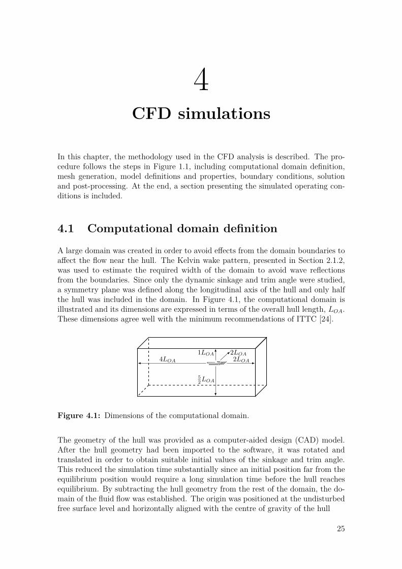
A large domain was created in order to avoid effects from the domain boundaries toaffect the flow near the hull. The Kelvin wake pattern, presented in Section 2.1.2,was used to estimate the required width of the domain to avoid wave reflectionsfrom the boundaries. Since only the dynamic sinkage and trim angle were studied,a symmetry plane was defined along the longitudinal axis of the hull and only halfthe hull was included in the domain. In Figure 4.1, the computational domain isillustrated and its dimensions are expressed in terms of the overall hull length, LOA.These dimensions agree well with the minimum recommendations of ITTC [24].

52LOA

1LOA2LOA4LOA

2LOA

Figure 4.1: Dimensions of the computational domain.

The geometry of the hull was provided as a computer-aided design (CAD) model.After the hull geometry had been imported to the software, it was rotated andtranslated in order to obtain suitable initial values of the sinkage and trim angle.This reduced the simulation time substantially since an initial position far from theequilibrium position would require a long simulation time before the hull reachesequilibrium. By subtracting the hull geometry from the rest of the domain, the do-main of the fluid flow was established. The origin was positioned at the undisturbedfree surface level and horizontally aligned with the centre of gravity of the hull

25

4. CFD simulations

4.2 Mesh generation

To capture the important flow phenomena in the simulations, the mesh density wasfocused on certain regions of the domain. First, a fine mesh was used on the hull sur-face and prism layers were created along the hull to resolve the boundary layer andto obtain correct shear stresses on the hull. The prism layers were constructed witha total thickness corresponding to the estimated boundary layer thickness, and theheight of the first cell layer was set to get a proper value of y+. Secondly, to resolvethe free surface accurately, a high mesh density was used in the region around thefree surface where the hull induced wakes were expected to be present. To preventsmearing of the free surface in front of the hull, a uniform cell height was used atthe free surface. Outside these regions, the mesh was coarser.

The mesh used in FLUENT was created using ANSYS Meshing. It was dividedinto two regions; one inner region of unstructured tetrahedral cells in a cuboidaround the hull, and one outer region of structured hexahedral cells. This meshstructure utilizes the flexibility of unstructured cells near the hull, while the numberof cells could be kept low with a structured mesh in the periphery of the domain.The interface between the structured and the unstructured regions was made non-conformal, meaning that the cell faces do not match at the interface, to keep thecell count low. In Figure 4.2, the structure of the FLUENT mesh is illustrated.

(a) Overview. (b) Symmetry plane.

(c) Prism layers. (d) Rail.

Figure 4.2: Schematic illustrations of the FLUENT mesh structure. (a) showsan overview of the mesh and (b) shows the mesh on the symmetry plane with theinner region of tetrahedral elements and the outer region of hexahedral elements.(c) shows the prism layers at the hull on the symmetry plane and (d) shows thetriangular surface mesh at a rail on the hull.

26

4. CFD simulations

The mesh constructed in STAR-CCM+ was divided into one stationary backgroundregion and one moving overset region close to the hull. Both parts were meshed withtrimmed, predominantly hexahedral cells with local refinements at the free surfaceand the wake. Since the whole overset region sinks and trims, thicker refinementzones around the free surface at the overlap were needed in order to maintain auniform cell height in front of the hull, which is seen in Figure 4.3b. Care had to betaken so that the cells in the overlapping region were of the same size and that theyformed a continuous layer around the overset region. In Figure 4.3, the structure ofthe STAR-CCM+ mesh is illustrated.

(a) Overview.

Overset regionOverlap

(b) Symmetry plane.

(c) Prism layers. (d) Rail.

Figure 4.3: Schematic illustrations of the STAR-CCM+ mesh structure. (a) showsan overview of the mesh and (b) shows the mesh on the symmetry plane with theoverset region and the background mesh. (c) shows the prism layers at the hull onthe symmetry plane and (d) shows the surface mesh at a rail on the hull.

4.3 Model definitions and propertiesThis section describes the mathematical models and numerical methods used in theCFD simulations.

4.3.1 Mathematical modelsBased on the theoretical background presented in Chapter 2, appropriate modelswere chosen for the simulations. These models were used for describing the two-phase flow and the interaction between the flow and the hull.

27

4. CFD simulations

4.3.1.1 Two-phase flow models

The turbulence was modelled using the RANS equations with the SST k-ω tur-bulence model. Wall functions were used in order to avoid resolving the wholeboundary layer. In FLUENT, blended wall functions were used, and the all y+ walltreatment was used in STAR-CCM+. Both these methods use a blend of low andhigh y+ wall functions and are suitable for a wide range of y+ values. The first layerthickness was set to obtain a y+ value around 100.

The free surface was modelled and resolved with the VOF method. The fluid prop-erties were set to be the same as in the model experiments that were used to validatethe results. Both the air and water were assumed to be incompressible.

4.3.1.2 Hull motion

To enable the 6 DOF solver to solve the equations of motion and rotation, the massand the moments of the inertia were specified. The moments of inertia were esti-mated using a flat plate with the same outer dimensions as the hull. Since onlythe heave and pitch motions of the hull were simulated, the 6 DOF solver of thesoftware was limited to 2 DOF. This was done by only allowing translational motionalong the z-axis and rotational motion around the y-axis. To account for the pullingmechanism used in a towing tank, an additional force had to be included in the 6DOF solver as this towing force induces an additional torque around the centre ofmass. It was assumed that the pulling mechanism exerted a horizontal force on thehull, meaning that the towing force had no components in the y- and z-directions.When the hull is towed at constant speed, the towing force magnitude is thus equalto the total resistance of the hull. Therefore, a force with the same magnitude asthe resistance but with opposite direction was applied in the towing point of thehull in each time step.

In FLUENT, the towing force was incorporated using a user defined function (UDF)which looped through all cell faces on the hull and summarized the friction andpressure forces acting in the horizontal direction. When the total force was known,the resulting torque could be calculated from the trim angle and the distance betweenthe towing point and the centre of gravity. This torque was applied in the UDF ofthe 6 DOF solver. In STAR-CCM+, the horizontal component of the resistance wasreported using a field function that calculates the friction and pressure forces on thehull surface. This force was then applied in the towing point as an external force.

4.3.2 Numerical methodsAfter the mathematical models had been chosen, numerical methods were selectedin the software. When choosing spatial discretization schemes, the second orderupwind scheme was chosen for all convection terms except for the volume fractionequation, where the compressive scheme was used in FLUENT and the HRIC schemewas used in STAR-CCM+. The diffusion terms were discretized with the centraldifferencing scheme. Since the steady behaviour of the hull was simulated and tem-

28

4. CFD simulations

poral accuracy was not important, the first order implicit scheme was chosen in thetemporal discretization. For the pressure-velocity coupling, the SIMPLE algorithmwas used.

The mesh motion in FLUENT was modelled using diffusion-based smoothing with adiffusion parameter of 1.5. To stabilize the fluid-structure interaction, the solutionstabilization option was enabled. In STAR-CCM+, the overset mesh method wasused.

4.4 Boundary conditions

The boundaries of the computational domain are illustrated in Figure 4.4. Thesymmetry plane as well as the top, side and bottom of the domain were prescribedwith symmetry boundary conditions, and the hull was set to a wall with no-slip.

Air inlet

Waterinlet

Outlet

Top

Bottom

Symmetry plane

Side

Figure 4.4: Boundaries of the computational domain.

At the inlet, located in front of the hull, the velocity of the incident air and waterwas set to the hull speed that was simulated. The turbulent flow variables were setby specifying values of the turbulent intensity and turbulent viscosity ratio. Theoutlet, located behind the hull, was set to a pressure outlet.

The location of the free surface was defined using the open channel flow model inFLUENT, and in STAR-CCM+ the level of the free surface was set with a coordi-nate and a normal vector. The static pressure at the inlet and outlet boundariescould thereby be obtained from the free surface location by specifying an atmo-spheric reference pressure in a point located above the free surface.

An undesired phenomenon that is often observed in hull simulations is a thin layerof air in the first cell layers at the hull surface. This air layer, which affects theshear stresses on the hull, emerges from the region where the free surface hits thehull. It is not observed in experiments, and any air layer forming in the first celllayers at the hull should therefore be removed. In FLUENT, a UDF was used toloop through the prism layer adjacent to the hull while the volume fraction of airwas set to 0 if it was below 0.3. In STAR-CCM+ a sink term was added to thetransport equation for the volume fraction. The sink term was applied in the cellsclosest to the hull where the volume fraction of air was below 0.3.

29

4. CFD simulations

4.5 SolutionThe inlet boundary conditions were used to initialize the flow field. Although asteady state solution was expected, transient simulations were run to enable meshmotion and increase the robustness of the solution. The iterative solution procedurewas first run with a fixed sinkage and trim in order to prevent large motions of thehull when the flow field was developed from the initial condition. When the hullwas released, the solution was run until the sinkage, trim angle and forces actingon the hull had stabilized around constant values. Since these measured values keptoscillating with relatively small amplitudes around the equilibrium values, the sim-ulation was continued for some time in order to sample enough data for accuratepredictions. The sampled data was processed by calculating the average values andthe corresponding standard errors. By doing this, confidence intervals for the esti-mations could be determined. The methods used for the data analysis are describedin Appendix A.

4.6 Post-processingWhen results had been obtained from a simulation, they were analysed and com-pared and new simulations were set up. In this iterative procedure, appropriatesettings for the simulations were found. Grid dependence studies were conducted inorder to estimate the numerical uncertainty.

4.7 Simulated operating conditionsThe CFD simulations were performed on two different hulls – the hull R/V ATHENA,hereafter referred to as the Athena hull, and a hull designed by Swede Ship, referredto as the Swede Ship hull.

4.7.1 Athena hullThe Athena hull was chosen because experimental data from model tests was avail-able. Therefore, the models and setup used in the CFD simulations could be vali-dated. The Athena hull is a large semi-planing hull with a full scale LPP of 46.9m.In the simulations, which were only performed using STAR-CCM+, a 1:8.556 scalemodel was used. Since the hull does not trim a lot the tow force was neglected.

A grid dependence study was conducted at a Froude number of 0.545 which corre-sponds to a velocity of 7.78 knots and a length between perpendiculars of 5.48m.There were some uncertainties in the exact position of the centre of gravity of thehull, both for the Athena and the Swede Ship hull. Therefore two cases, CG1 andCG2, with different positions of the centre of gravity were simulated for Athena inorder to get an idea of how sensitive the results are to the position of centre of grav-ity. Figure 4.5 shows the outline of the hull with the location of the two differentcentres of gravity used for the simulations. The dimensions of the Athena hull are

30

4. CFD simulations

found in Table 4.1 and the fluid properties used in the simulations are presented inTable 4.2.

• CG2• CG1 Waterline

x

z

⊗y

Figure 4.5: Sketch of the Athena hull showing the two different centres of gravity,CG1 and CG2, used in the simulations.

Table 4.1: Hull dimensions of R/V Athena. A model scale with scaling factor1:8.556 was used in the simulations. Two different centres of gravity were simulated,CG1 and CG2.

Description Symbol ValueLength between perpendiculars LPP 46.9mVolume displacement ∇ 257.5m3

Longitudinal CG from AP, CG1 LCG 20.16mLongitudinal CG from AP, CG2 LCG 17.97mVertical CG, CG1 V CG 2.396mVertical CG, CG2 V CG 0.684m

Table 4.2: Fluid properties used in the simulations of the Athena hull.

Description Symbol ValueAtmospheric pressure at water surface Patm 101325PaDensity of water ρw 998.83 kg/m3

Viscosity of water νw 8.8871×10−4 m2/sDensity of air ρa 1.18415 kg/m3

Viscosity of air νa 1.85508×10−5 m2/s

4.7.2 Swede Ship hullThe Swede Ship hull is a planing hull with an LPP of 13.5m. The simulationswere conducted in full scale, and the hull dimensions and fluid properties used inthe simulations are found in Table 4.3 and Table 4.4. A more detailed table withproperties is presented in Appendix C.

31

4. CFD simulations

Table 4.3: Properties and dimensions of the Swede Ship hull at a water density of1025.87 kg/m3 and a shell plating thickness of 8.00mm.

Description Symbol ValueLength between perpendiculars LPP 13.500mBreadth waterline BWL 4.157mVolume displacement ∇ 22.8m3

Longitudinal CG from AP LCB 4.921mVertical CG V CG 1.9mVertical CB V CB 0.6785m

Table 4.4: Fluid properties used in the simulations of the Swede Ship hull.

Description Symbol ValueAtmospheric pressure at water surface Patm 101325PaDensity of water ρw 1025.87 kg/m3

Viscosity of water νw 1.188×10−6 m2/sDensity of air ρa 1.225 kg/m3

Viscosity of air νa 1.461×10−5 m2/s

The simulations of the Swede Ship hull were performed both with fixed and freesinkage and trim. The purpose of the fixed sinkage and trim simulations was to ob-tain a detailed comparison of the results from FLUENT and STAR-CCM+. Thesesimulations were conducted at a Froude number of 1.68 with a sinkage at LPP/2of 0.685m and a trim angle of 3.19 that were determined from a free sinkage andtrim simulation in STAR-CCM+.

In the simulations with free sinkage and trim, the Swede Ship hull was simulatedwith a centre of gravity and a centre of buoyancy as shown in Figure 4.6. The centreof gravity was provided in the hull data, and the towing point was stated to be inthe centre of buoyancy at zero speed. In order to find the centre of buoyancy, thehull data was used to position the hull in its zero speed position, and then the centreof mass of the displaced volume was calculated. Due to some uncertainties in theexact position of the centre of gravity in the vertical direction, one simulation wasperformed where it was shifted 0.1m up. The results for the two cases, CG1 andCG2, were compared in order to evaluate if, and how much, the uncertain positionof the centre of gravity affects the results.

•CG

•CB

Waterline

x

z

⊗y

Figure 4.6: Sketch of the Swede Ship hull showing the centre of gravity (CG) andthe centre of buoyancy (CB) at zero speed.

32

4. CFD simulations

The free sinkage and trim simulations were conducted at Froude numbers rangingfrom 0.447 to 1.79, corresponding to velocities of 10 knots to 40 knots. A summaryof the simulated cases is shown in Table 4.5 and Table 4.6. After the final resultswere obtained, they were compared with experimental data.

Table 4.5: Simulated cases for the Swede Ship hull with fixed sinkage and trim.

Fn Velocity [knots]Mesh study, FLUENT 1.68 37.5FUENT 1.68 37.5STAR-CCM+ 1.68 37.5

Table 4.6: Simulated cases for the Swede Ship hull with free sinkage and trim.

Fn Velocity [knots]Mesh Study, STAR-CCM+ 1.68 37.5STAR-CCM+, CG1 1.68 37.5STAR-CCM+, CG2 1.68 37.5STAR-CCM+ 1.79 40.0STAR-CCM+ 1.68 37.5STAR-CCM+ 1.57 35.0STAR-CCM+ 1.34 30.0STAR-CCM+ 1.12 25.0STAR-CCM+ 0.894 20.0STAR-CCM+ 0.671 15.0STAR-CCM+ 0.447 10.0FLUENT 1.68 37.5

33

4. CFD simulations

34

5Results and discussion

This chapter presents the results from the CFD simulations performed as describedin Chapter 4. The results are divided into three parts: free sinkage and trim sim-ulations of the Athena hull, fixed sinkage and trim simulations of the Swede Shiphull and free sinkage and trim simulations of the Swede Ship hull.

5.1 Athena hullIn the following sections the results from the simulations in STAR-CCM+ of theAthena hull with free sinkage and trim are presented and compared with experimen-tal data. Two cases, CG1 and CG2, with different locations of the centre of gravitywere simulated. The simulations were performed at a Froude number of 0.545. Firstthe grid dependence study is presented and then the comparison between experi-mental data and the calculated properties is presented and discussed.

5.1.1 Grid dependence studyThe grid dependence study was carried out for CG1. The grid was systematicallyrefined in steps resulting in six different meshes. The number of cells for the coarsestmesh was 0.287 million and the finest mesh had 11.9 million cells. The number ofcells for all meshes is presented in Table D.1 in Appendix D. The convergence of thetotal resistance coefficient was studied and the results are presented in Figure 5.1.It shows that the second finest grid with 7.10 million cells is a good compromisebetween numerical accuracy and computational effort. This mesh has a numericaluncertainty of 1.3% and was used to simulate CG2.

35

5. Results and discussion

0 0.5 1 1.5 2 2.5 3 3.5 46.2

6.3

6.4

6.5

6.6

6.7

x 10−3

3√N1/N i

CT

ComputedFitted curve

Figure 5.1: Convergence of the total resistance coefficient with grid refinement forthe free sinkage and trim simulations of the Athena hull performed in STAR-CCM+at Fn = 0.545. The full circle represents the grid used for simulating CG2.

5.1.2 Calculated propertiesThe computed properties for the two cases are presented and compared with exper-imental data in Table 5.1. It is seen that the results from the simulation of CG1give a lower sinkage and trim angle and underpredict the resistance compared tothe experimental results. The results from CG2 give a sinkage that is closer to theexperimental value but the trim angle is larger and the resistance is overpredicted.The results indicate that the chosen models and setup are appropriate.

Table 5.1: Experimental and calculated properties of the Athena hull with freesinkage and trim at Fn = 0.545.

Experiment CG1 CG2Resistance [N] 244.52 229.14 ± 0.01 255.39 ± 0.22Error -6.31% 4.25%Sinkage [m] -0.0105 -0.00874 ± 0.00010 -0.00968 ± 0.00017Error -16.56% -4.44%Trim angle [] 1.35 1.26 ± 0.00 1.50 ± 0.00Error -6.76% 10.05%

Athena is a semi-planing hull, and as seen in Table 5.1 the sinkage and trim angleare very small. A much higher mesh density is needed than what was used in thesesimulations to be able to obtain the exact position of the hull. Figure 5.2 shows thevolume fraction of air around the hull at the symmetry plane.

36

5. Results and discussion

Volume fraction of air, γ0 0.2 0.4 0.6 0.8 1.0

x

z

⊗y

Figure 5.2: Volume fraction of air at the symmetry plane of the Athena hull atFn = 0.545.

It is seen in the results that the position of the centre of gravity affects the calculatedresistance, sinkage and trim. Another reason to why the calculated values differ fromthe experimental values is that the towing force was neglected. This implies thatit is important to know exactly how the experiments were performed in order toobtain accurate and reliable results.

37

5. Results and discussion

5.2 Swede Ship hull, fixed sinkage and trimThe following sections present the results from the simulations with fixed sinkageand trim for the Swede Ship hull. The hull speed was set to 37.5 knots, correspond-ing to a Froude number of 1.68, and the sinkage at LPP/2 and trim angle were0.685m and 3.19, respectively. After a presentation of the grid dependence study,the calculated volume fraction distribution, pressure coefficient, skin friction coeffi-cient, dimensionless wall distance and free surface pattern are visualized. At the end,the calculated forces acting on the hull and the wetted area and length are presented.

When cross sections are used to present the results, they have been constructedfrom planes as illustrated in Figure 5.3. According to this figure, two longitudinalcross sections run along the hull surface at y/LPP = 0.0037 and y/LPP = 0.037, twolongitudinal cross sections are placed outside the hull at y/LPP = 0.30 and y/LPP =0.37, and two transverse cross sections run across the hull at x/LPP = −0.22 andx/LPP = −0.15.

Symmetryy/LP P = 0.0037y/LP P = 0.037

y/LP P = 0.30y/LP P = 0.37

x/LP P = −0.22x/LP P = −0.15

•O

x

y

⊗z

Figure 5.3: Cross sections at different y-coordinates used in the illustrations of theresults. The origin of the computational domain is marked by O, and its position isin level with the undisturbed free surface.

5.2.1 Grid dependence studyFour meshes with a cell count ranging from 4.28 million to 24.2 million cells were usedin the grid dependence study conducted in Fluent. In Table D.2 in Appendix D,the number of cells in each mesh are presented. The calculated total resistancecoefficients for these meshes are presented in Figure 5.4. The second finest meshwith 16.9 million cells and a numerical uncertainty of 1.7% was chosen for furtheranalysis. In STAR-CCM+, a mesh with 18.4 million cells was selected based on agrid dependence study for free sinkage and trim. Consequently, the meshes used inthe following comparison of the results in FLUENT and STAR-CCM+ have similarcell counts.

38

5. Results and discussion

0 0.5 1 1.5 22.85

2.9

2.95

3

3.05

3.1x 10

−3

3√N1/Ni

CT

ComputedFitted curve

Figure 5.4: Convergence of the total resistance coefficient with grid refinement forthe fixed sinkage and trim simulations of the Swede Ship hull performed in FLUENTat Fn = 1.68. The full circle represents the grid used in the further analysis.

5.2.2 Volume fraction of air at the hullIn Figure 5.5, contour plots of the volume fraction of air on the hull are presented.The differences between the results obtained in FLUENT and STAR-CCM+ arefound where the free surface hits the hull. In particular, the region around thesymmetry plane shows large differences. The air at the symmetry in both cases andat the rails in STAR-CCM+ is due to that the air that hits the hull at the freesurface is dragged down along the hull. This phenomenon is prevented by removingair from cells which has a volume fraction of water higher than 0.7. As seen inthe contour plots, more air could be removed, but then some realistic air might beremoved and the sides of the hull can get unrealistically wet. The areas with volumefraction of air around 0.7 in the left picture might be due to splashing water. Thearea that is completely covered by water has the same shape in the two cases.

Volume fraction of air, γair

0 0.2 0.4 0.6 0.8 1.0

(a) FLUENT (b) STAR-CCM+

x

y

⊗z

Figure 5.5: Contour plots of the volume fraction of air on the hull for the fixedsinkage and trim simulations at Fn = 1.68.

39

5. Results and discussion

5.2.3 Pressure coefficientFigure 5.6 shows contour plots of the pressure coefficient on the hull. The resultsfrom FLUENT and STAR-CCM+ agree very well, and no apparent differences canbe identified. A spot of significantly higher pressure is observed where the freesurface hits the second innermost rail on the hull.

Pressure coefficient, CP

0 0.08 0.16 0.24 0.32 0.40

(a) FLUENT (b) STAR-CCM+

x

y

⊗z

Figure 5.6: Contour plots of the pressure coefficient on the hull for the fixed sinkageand trim simulations at Fn = 1.68.

In Figure 5.7, longitudinal cross sections of the pressure coefficient on the hull areshown. In these plots, the similarity between the results is very clear – the curvesbarely differ from each other in the two cross sections.

−0.4 −0.2 0 0.2 0.40

0.02

0.04

0.06

0.08

0.1

0.12

CP

x/LPP

FLUENTSTAR-CCM+

(a) y/LPP = 0.0037.

−0.4 −0.2 0 0.2 0.40

0.02

0.04

0.06

0.08

0.1

0.12

CP

x/LPP

FLUENTSTAR-CCM+

(b) y/LPP = 0.037.

Figure 5.7: Longitudinal cross sections of the pressure coefficient on the hull forthe fixed sinkage and trim simulations at Fn = 1.68.

In Figure 5.8, transverse cross sections of the pressure coefficient on the hull areshown. It can be observed that the pressure predicted by FLUENT is higher inthe outer region of the hull around the lifting rails. The origin of this difference isnot known, but it indicates that the regions around the lifting rails require specialattention.

40

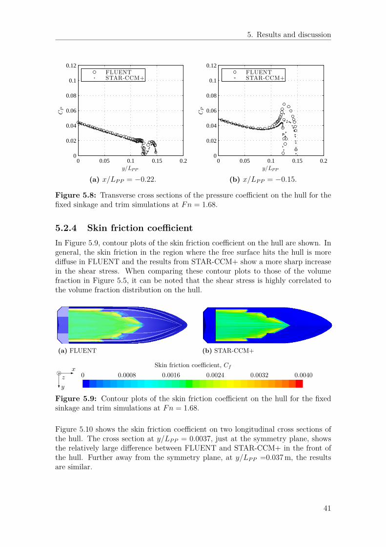
5. Results and discussion

0 0.05 0.1 0.15 0.20

0.02

0.04

0.06

0.08

0.1

0.12C

P

y/LPP

FLUENTSTAR-CCM+

(a) x/LPP = −0.22.

0 0.05 0.1 0.15 0.20

0.02

0.04

0.06

0.08

0.1

0.12

CP

y/LPP

FLUENTSTAR-CCM+

(b) x/LPP = −0.15.

Figure 5.8: Transverse cross sections of the pressure coefficient on the hull for thefixed sinkage and trim simulations at Fn = 1.68.

5.2.4 Skin friction coefficientIn Figure 5.9, contour plots of the skin friction coefficient on the hull are shown. Ingeneral, the skin friction in the region where the free surface hits the hull is morediffuse in FLUENT and the results from STAR-CCM+ show a more sharp increasein the shear stress. When comparing these contour plots to those of the volumefraction in Figure 5.5, it can be noted that the shear stress is highly correlated tothe volume fraction distribution on the hull.

Skin friction coefficient, Cf

0 0.0008 0.0016 0.0024 0.0032 0.0040

(a) FLUENT (b) STAR-CCM+

x

y

⊗z

Figure 5.9: Contour plots of the skin friction coefficient on the hull for the fixedsinkage and trim simulations at Fn = 1.68.

Figure 5.10 shows the skin friction coefficient on two longitudinal cross sections ofthe hull. The cross section at y/LPP = 0.0037, just at the symmetry plane, showsthe relatively large difference between FLUENT and STAR-CCM+ in the front ofthe hull. Further away from the symmetry plane, at y/LPP =0.037m, the resultsare similar.

41

5. Results and discussion

−0.4 −0.2 0 0.2 0.40

1

2

3

4x 10

−3

Cf

x/LPP

FLUENTSTAR-CCM+

(a) y/LPP = 0.0037.

−0.4 −0.2 0 0.2 0.40

1

2

3

4x 10

−3

Cf

x/LPP

FLUENTSTAR-CCM+

(b) y/LPP = 0.037.

Figure 5.10: Longitudinal cross sections of the skin friction coefficient on the hullfor the fixed sinkage and trim simulations at Fn = 1.68.

5.2.5 Dimensionless wall distanceFigure 5.11 shows contour plots of the dimensionless wall distance at the hull. Sincethe regions of air were not taken into account when choosing the first layer thicknessof the prism layers, the y+ values are not close to the target value of 100 where airflows at the hull. However, since the air resistance constitutes a very small part ofthe total friction resistance, this deviation is of little importance.

Dimensionless wall distance, y+

0 30 60 90 120 150

(a) FLUENT (b) STAR-CCM+

x

y

⊗z

Figure 5.11: Contour plots of the dimensionless wall distance on the hull for thefixed sinkage and trim simulations at Fn = 1.68.

42

5. Results and discussion

5.2.6 Free surface wave patternIn Figure 5.12, the dimensionless height of the free surface is shown. The free surfaceis defined as the interface between water and air where the volume fractions are 0.5.The wake patterns predicted by FLUENT and STAR-CCM+ are similar, but theresult obtained in STAR-CCM+ shows more details near the hull. This is probablybecause of a higher mesh density around the hull in STAR-CCM+, where moreeffort was put into the construction of an appropriate mesh in this region.

Dimensionless free surface height, z/LP P

-0.060 -0.036 -0.012 0.012 0.036 0.060

(a) FLUENT (b) STAR-CCM+

x

y

z

Figure 5.12: Contour plots of the dimensionless free surface height for the fixedsinkage and trim simulations at Fn = 1.68. z/LPP = 0 is the height of the undis-turbed free surface.

Figure 5.13 shows longitudinal cross sections of the free surface height outside thehull. In these figures it is clearer that the mesh created in STAR-CCM+ capturesmore of the waves and the splashing close to the hull. Further away from the hull,the results are similar.

43

5. Results and discussion

−4 −3 −2 −1 0 1 2−0.05

0

0.05z/

LPP

x/LPP

FLUENTSTAR-CCM+

(a) y/LPP = 0.30.

−4 −3 −2 −1 0 1 2−0.05

0

0.05

z/LPP

x/LPP

FLUENTSTAR-CCM+

(b) y/LPP = 0.37.

Figure 5.13: Cross sections of the dimensionless free surface height at Fn = 1.68.z/LPP = 0 is the height of the undisturbed free surface.

5.2.7 Calculated propertiesThe calculated properties are presented in Table 5.2. It shows that there is a signif-icant difference in the calculated pressure force between the two simulations. Thevalue obtained in FLUENT is 13% higher than the value from STAR-CCM+. Fromthe comparisons of the pressure coefficient in Section 5.2.3, this difference stemsfrom the sides of the hull around the lifting rails. Due to this difference, the totalresistance prediction differs by 8.0%. Apart from the pressure resistance, the resultsfrom FLUENT and STAR-CCM+ show good correspondence.

Table 5.2: Calculated properties of the Swede Ship hull with fixed sinkage atLPP/2 and trim angle of 0.685m and 3.19, respectively, at Fn = 1.68.

STAR-CCM+ FLUENT DifferencePressure resistance [N] 17606 ± 1 19962 ± 1 13%Friction resistance [N] 11057 ± 2 10991 ± 0 -0.60%Total resistance [N] 28663 ± 2 30954 ± 1 8.0%Lift force [N] 217760 ± 20 220400 ± 10 1.2%Wetted area [m2] 30.31 ± 0.00 29.76 ± 0.00 -1.8%Wetted length [m2] 9.45 ± 0.00 9.37 ± 0.00 -0.85%

According to Larsson and Raven [10, p. 154], the pressure resistance is sensitiveto the mesh density. When the meshes used in FLUENT and STAR-CCM+ werecompared, no clear differences in terms of cell size could be identified at the rails.

44

5. Results and discussion

5.3 Swede Ship hull, free sinkage and trimThe following sections present the results from the simulations with free sinkageand trim for the Swede Ship hull, which were mainly conducted in STAR-CCM+.First, the grid dependence study for Fn = 1.68 is presented and then the resultsfrom the simulations with two different positions of centre of gravity are compared.Then, the results from the calculations of the Froude number dependencies of theresistance, sinkage, trim angle, wetted area and wetted length are compared withexperimental data. Results from FLUENT were only obtained for one speed due toproblems with the simulations, which are discussed in the end of this chapter.

5.3.1 Grid dependence studyFive different meshes with the number of cells ranging between 0.989 million and 38.2million cells were used in the study, the number of cells of each mesh are presented inTable D.3 in Appendix D. The results for the total resistance coefficient are presentedin Figure 5.14a. Figure 5.14b shows the difference in calculated values comparedto the finest mesh which is mesh number 1. CT converges to an asymptotic valueand the differences between the meshes are small. The results for sinkage and trimangle are presented in Figure 5.15 and Figure 5.16. Here, the convergence is not asclear as for the total resistance coefficient and the differences between the meshesare larger, especially for the trim angle.

0 1 2 3 4

2.7

2.8

2.9

3

3.1

3.2x 10

−3

3√

N1/Ni

CT

ComputedFitted curve

(a) Total resistance coefficient.

1 2 3 4 5−3

−2.5

−2

−1.5

−1

−0.5

0

0.5

Mesh number

Differen

ce[%

]

(b) Difference between the meshes.

Figure 5.14: Convergence of the total resistance coefficient with grid refinementfor the free sinkage and trim simulations of the Swede Ship hull performed inSTAR-CCM+ at Fn = 1.68. The calculated values for each mesh are comparedto the densest mesh which is mesh 1.

45

5. Results and discussion

0 1 2 3 40.6

0.65

0.7

3√

N1/Ni

s[m

]

ComputedFitted curve

(a) Sinkage.

1 2 3 4 5−2

−1.5

−1

−0.5

0

0.5

1

Mesh number

Differen

ce[%

]

(b) Difference between the meshes.

Figure 5.15: Convergence of the sinkage with grid refinement for the free sinkageand trim simulations of the Swede Ship hull performed in STAR-CCM+ at Fn =1.68. The calculated values for each mesh are compared to the densest mesh whichis mesh 1.

0 1 2 3 42.5

3

3.5

4

4.5

3√

N1/Ni

θ[]

ComputedFitted curve

(a) Trim.

1 2 3 4 5

0

2

4

6

8

10

Mesh number

Differen

ce[%

]

(b) Difference between the meshes.

Figure 5.16: Convergence of the trim angle with grid refinement for the freesinkage and trim simulations of the Swede Ship hull performed in STAR-CCM+ atFn = 1.68. The calculated values for each mesh are compared to the densest meshwhich is mesh 1.

The second finest grid with 18.4 million cells has a numerical uncertainty of 0.13%and was used for the simulations of fixed sinkage and trim and for the comparisonwith a shifted centre of gravity. Mesh number 3 has a numerical uncertainty of0.19% and was used for the simulations with different Froude numbers.

46

5. Results and discussion

5.3.2 Centre of gravity sensitivity analysisThe centre of gravity was shifted 0.1m up compared to the original position, CG1.The simulation of CG2 was performed at Fn = 1.68 and mesh number 2 was used.The results are summarized in Table 5.3 and it is seen that there are differences intrim angle and wetted length while the other differences are small.

Table 5.3: Calculated properties of the Swede Ship hull with free sinkage and trimat Fn = 1.68.

CG1 CG2 DifferenceTotal resistance [N] 30640 ± 7 30404 ± 73 -0.77%Lift force [N] 229380 ± 20 227880 ± 600 -0.56%Sinkage Lpp/2 [m] 0.676 ± 0.005 0.684 ± 0.190 -0.98%Trim angle[] -3.52 ± 0.00 -3.31 ± 0.02 -5.7%Wetted area [m2] 30.61 ± 0.01 30.82 ± 0.08 -0.70%Wetted length [m] 9.20 ± 0.01 10.1 ± 0.4 9.8%

This indicates that the results are not very sensitive to vertical translations of thecentre of gravity. Nevertheless, accurate predictions require a precise specificationof the centre of gravity.

5.3.3 Calculated propertiesThe Froude number simulations were conducted in STAR-CCM+, where the thirdmesh from the grid dependence study for free sinkage and trim with 5.64 millioncells was used. One simulation was conducted in FLUENT for Fn = 1.68, where themesh with 16.9 million cells from the fixed sinkage and trim simulations was used.In Figure 5.17-5.21, the results for total resistance, sinkage, trim angle, wetted areaand wetted length obtained with CFD are compared to the values from experimentalfluid dynamics (EFD).

The results for the total hull resistance are shown in Figure 5.17. It is seen thatthe calculated results follows the experimental values and that the error is between-8.2% and 6.5% for STAR-CCM+. The resistance is overpredicted in the transitionregion around Fn = 1 and underpredicted in the planing region. In FLUENT, theresistance is closer to the experimental value, the error is -1.1%.

47

5. Results and discussion

0 0.5 1 1.51

1.5

2

2.5

3

3.5

4x 10

4

Fn

Rtot[N

]

STAR−CCM+FLUENTEFD

(a) Total resistance.

0 0.5 1 1.5−20

−15

−10

−5

0

5

10

Fn

Error[%

]

STAR−CCM+FLUENT

(b) Error.

Figure 5.17: Computational and experimental results for the Froude number de-pendency of the total resistance for the Swede Ship hull with free sinkage and trim.

The calculated and experimental sinkage values at LPP/2 are compared in Fig-ure 5.18. It is seen that the CFD-simulations in STAR-CCM+ give a higher sinkagefor all Froude numbers. This may be due to that the assumption of a horizontaltowing force is not valid. The agreement is better in the planing region where theerror is around a few percent. In FLUENT, the sinkage is underpredicted by 6.6%.When looking at the error it should be noted that the values for the lower Froudenumbers are misleading since the sinkage is approaching zero. The error becomeslarger due to the small values of the sinkage. It is better to look at Figure 5.18awhere it is seen that the differences are not that large.

0 0.5 1 1.5−0.2

0

0.2

0.4

0.6

0.8

Fn

s[m

]

STAR−CCM+FLUENTEFD

(a) Sinkage at LPP/2.

0 0.5 1 1.5−60

−40

−20

0

20

40

Fn

Error[%

]

STAR−CCM+FLUENT

(b) Error.

Figure 5.18: Computational and experimental results for the Froude number de-pendency of the sinkage for the Swede Ship hull with free sinkage and trim.

48

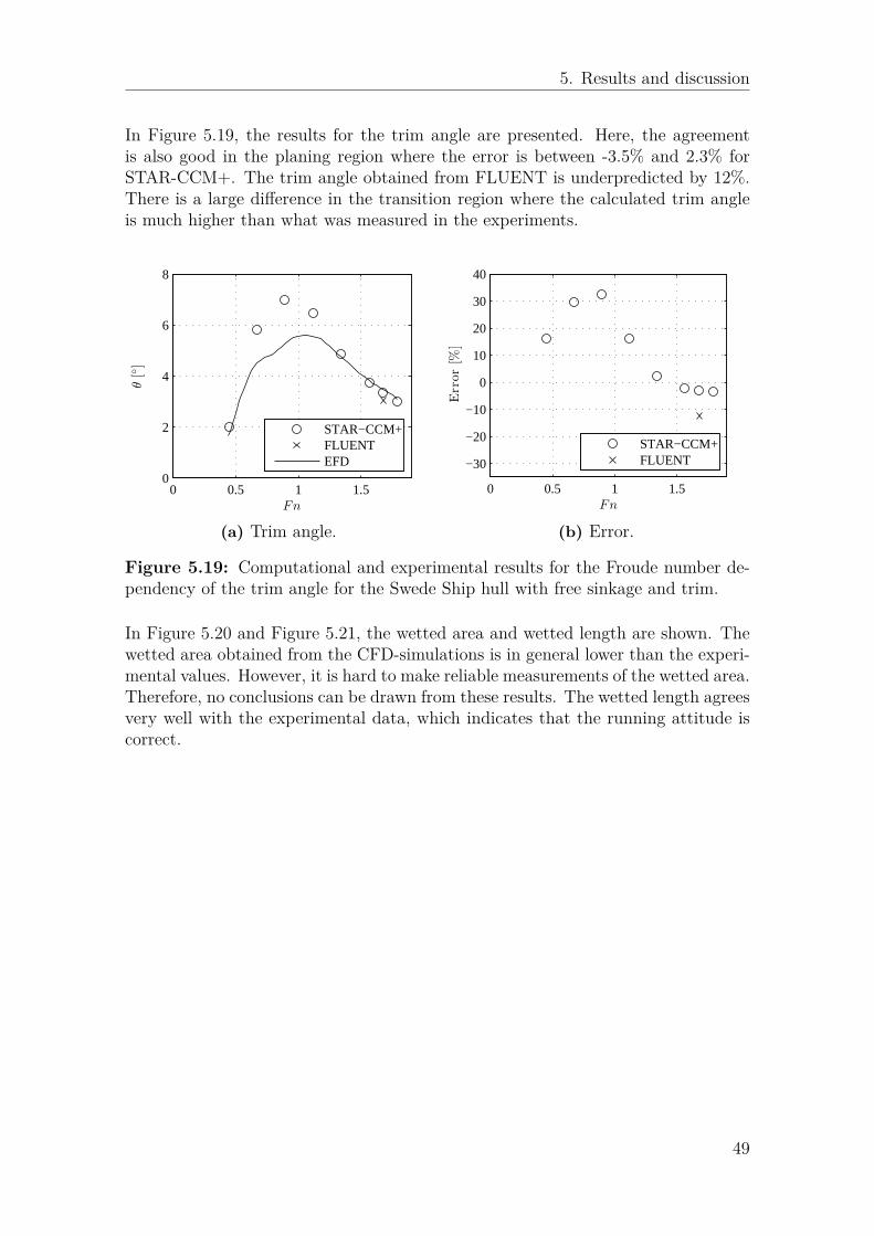
5. Results and discussion

In Figure 5.19, the results for the trim angle are presented. Here, the agreementis also good in the planing region where the error is between -3.5% and 2.3% forSTAR-CCM+. The trim angle obtained from FLUENT is underpredicted by 12%.There is a large difference in the transition region where the calculated trim angleis much higher than what was measured in the experiments.

0 0.5 1 1.50

2

4

6

8

Fn

θ[]

STAR−CCM+FLUENTEFD

(a) Trim angle.

0 0.5 1 1.5

−30

−20

−10

0

10

20

30

40

Fn

Error[%

]

STAR−CCM+FLUENT

(b) Error.

Figure 5.19: Computational and experimental results for the Froude number de-pendency of the trim angle for the Swede Ship hull with free sinkage and trim.

In Figure 5.20 and Figure 5.21, the wetted area and wetted length are shown. Thewetted area obtained from the CFD-simulations is in general lower than the experi-mental values. However, it is hard to make reliable measurements of the wetted area.Therefore, no conclusions can be drawn from these results. The wetted length agreesvery well with the experimental data, which indicates that the running attitude iscorrect.

49

5. Results and discussion

0 0.5 1 1.530

35

40

45

50

55

60

Fn

AW

[m2]

STAR−CCM+FLUENTEFD

(a) Wetted area.

0 0.5 1 1.5−20

−15

−10

−5

0

5

Fn

Error[%

]

STAR−CCM+FLUENT

(b) Error.

Figure 5.20: Computational and experimental results for the Froude number de-pendency of the wetted area for the Swede Ship hull with free sinkage and trim.

0 0.5 1 1.57

8

9

10

11

12

13

14

15

Fn

LW

[m]

STAR−CCM+FLUENTEFD

(a) Wetted length.

0 0.5 1 1.5−10

−5

0

5

10

Fn

Error[%

]

STAR−CCM+FLUENT

(b) Error.

Figure 5.21: Computational and experimental results for the Froude number de-pendency of the wetted length for the Swede Ship hull with free sinkage and trim.

Overall, the trends in the results are the same for the calculated and experimentalvalues. The position of the hull in terms of sinkage and trim angle is best predictedin the higher Froude number range. In this range the resistance is underpredicted.

50

5. Results and discussion

5.3.4 Free surface wave patternIn Figure 5.22, contour plots of the free surface height at three different Froudenumbers are shown. These have been chosen so that the first, Fn = 0.447, is inthe displacement region, the second, Fn = 0.894 is in the transition region and thethird, Fn = 1.68, is in the planing region.

Dimensionless free surface height, z/LP P

-0.060 -0.036 -0.012 0.012 0.036 0.060

(a) Fn = 0.447 (b) Fn = 0.447

(c) Fn = 0.894 (d) Fn = 0.894

(e) Fn = 1.68 (f) Fn = 1.68

Figure 5.22: Contour plots of the dimensionless free surface height for the freesinkage and trim simulations obtained in STAR-CCM+ at Fn = 0.447, Fn = 0.894and Fn = 1.68.

51

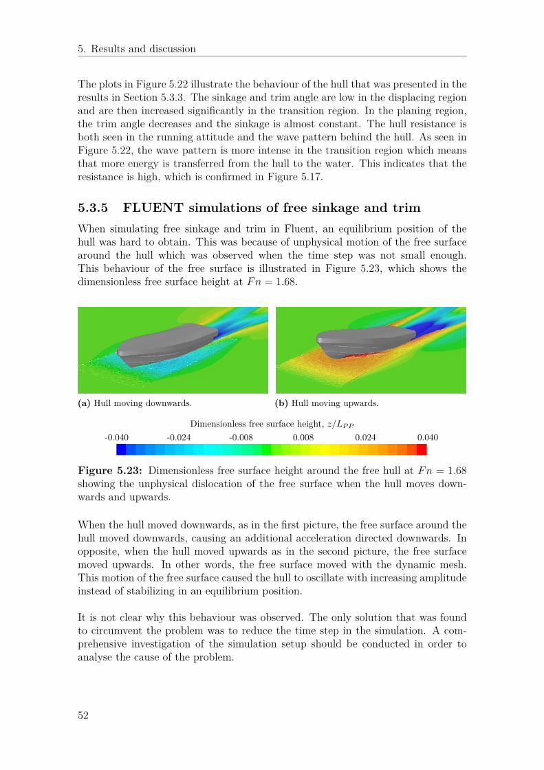
5. Results and discussion

The plots in Figure 5.22 illustrate the behaviour of the hull that was presented in theresults in Section 5.3.3. The sinkage and trim angle are low in the displacing regionand are then increased significantly in the transition region. In the planing region,the trim angle decreases and the sinkage is almost constant. The hull resistance isboth seen in the running attitude and the wave pattern behind the hull. As seen inFigure 5.22, the wave pattern is more intense in the transition region which meansthat more energy is transferred from the hull to the water. This indicates that theresistance is high, which is confirmed in Figure 5.17.

5.3.5 FLUENT simulations of free sinkage and trimWhen simulating free sinkage and trim in Fluent, an equilibrium position of thehull was hard to obtain. This was because of unphysical motion of the free surfacearound the hull which was observed when the time step was not small enough.This behaviour of the free surface is illustrated in Figure 5.23, which shows thedimensionless free surface height at Fn = 1.68.

(a) Hull moving downwards. (b) Hull moving upwards.

Dimensionless free surface height, z/LP P

-0.040 -0.024 -0.008 0.008 0.024 0.040

Figure 5.23: Dimensionless free surface height around the free hull at Fn = 1.68showing the unphysical dislocation of the free surface when the hull moves down-wards and upwards.

When the hull moved downwards, as in the first picture, the free surface around thehull moved downwards, causing an additional acceleration directed downwards. Inopposite, when the hull moved upwards as in the second picture, the free surfacemoved upwards. In other words, the free surface moved with the dynamic mesh.This motion of the free surface caused the hull to oscillate with increasing amplitudeinstead of stabilizing in an equilibrium position.

It is not clear why this behaviour was observed. The only solution that was foundto circumvent the problem was to reduce the time step in the simulation. A com-prehensive investigation of the simulation setup should be conducted in order toanalyse the cause of the problem.

52

6Conclusion

CFD simulations can provide data that is difficult to obtain from experiments, forexample streamlines around the hull and detailed distributions of the forces actingon the hull. Therefore, CFD can be used by shipyards in order to make improve-ments and corrections at an early stage in the design process. Whether CFD canreplace towing tank tests or not, is not only a matter of the accuracy of the results.In addition, the simulations must either be faster or cost less than a correspondingexperimental analysis.

The results from the CFD simulations of free sinkage and trim obtained in STAR-CCM+ are similar to the behaviour that is seen in the experimental data. Theresistance is underpredicted in the planing region, at Froude numbers higher than1.3, and the results deviate by 6.1% to 8.2%. The sinkage is overpredicted for allFroude numbers, but is closer to the experimental data in the planing region wherethe difference is between 0.33% to 9.7%. The trim angle was hard to predict in thetransition region of Froude numbers around 1, where it is overpredicted by up to32%. In the planing region the agreement is better and the deviation is between-3.5% and 2.3%. The wetted area shows a large deviation in the planing area, con-sidering the agreement with the running attitude. However, the wetted length showsa better correspondence to the experimental values. The accuracy of the results isin line with earlier studies of planing hulls.

The results obtained in the simulations of fixed sinkage and trim in FLUENT andSTAR-CCM+ are in good agreement. However, there is a difference in pressure re-sistance which probably originates from the sides of the hull, where a higher pressureis predicted by FLUENT. This leads to a higher total resistance, which is interestingsince the results from STAR-CCM+ show that the resistance is underpredicted ata similar running attitude. In FLUENT, only one free sinkage and trim simula-tion could be performed due to problems with free surface dislocation during meshmotion. Compared to the results from STAR-CCM+, the calculated resistance iscloser to the experimental values whereas the sinkage and trim angle deviate more.It would be valuable to obtain results for other Froude numbers from FLUENT tobe able to compare the methods and models used in the software.

53

6. Conclusion

54

7Future work

Future work should focus on a detailed investigation on the mesh distribution closeto the hull to make sure that all the important features, like wave breaking andspray, are captured. Grid dependence studies can be done to study the influenceof first layer cell height and the number of cells in the prism layer on the results.Moreover, grid dependence studies should be done for all Froude numbers to get anoptimal mesh that captures the important phenomena in each case. It would alsobe of interest to examine the difference in pressure resistance between the resultsfrom FLUENT and STAR-CCM+.

55

7. Future work

56

References

[1] Holtrop, J., Mennen, G. G. J. A Statistical Power Prediction Method. Inter-national Shipbuilding Progress. 1978;25(290):253–256.

[2] Savitsky, D., Brown, P. W. Procedures for Hydrodynamic Evaluation of Plan-ing Hulls in Smooth and Rough Water. Marine Technology. 1976;13(4):381–400.

[3] Brizzolara, S., Serra, F. Accuracy of CFD Codes in the Prediction of Plan-ing Surfaces Hydrodynamic Characteristics. 2nd International Conference onMarine Research and Transportation. Ischia; 2007.

[4] Azcueta, R. Computation of Turbulent Free-Surface Flows Around Ships andFloating Bodies. PhD thesis. Hamburg: Technical University of Hamburg;2001.

[5] Larsson, L., Stern, F., Visonneau, M. Numerical Ship Hydrodynamics - AnAssessment of the Gothenburg 2010 Workshop. Dordrecht: Springer; 2013.

[6] Brizzolara, S., Villa, D. CFD Simulations of Planing Hulls. 7th InternationalConference on High-Performance Marine Vehicles. Melbourne; 2010.

[7] Visone, M., Bertetti, P., Gandolfi, R., Falletta, C., Ausonio, P. L., Paterna,D., et al. VOF-Dynamic Mesh Simulations of Unsteady Ship Hydrodynamics.Marine CFD 2005 - 4th International Conference on Marine Hydrodynamics.London: The Royal Institution of Naval Architects; 2005.

[8] Caponnetto, M., Bučan, B., Pedišić-Buča, M., Perić, M., Pettinelli, C. Sim-ulation of Flow and Motion of High-Speed Vessels. Proceedings of the 12thInternational Conference on Fast Sea Transportation. Amsterdam; 2013.

[9] Fu, T. C., Brucker, K. A., Mousaviraad, S. M., Ikeda, C. M., Lee, E. J., O’Shea,T. T., et al. An Assessment of Computational Fluid Dynamics Predictions ofthe Hydrodynamics of High-Speed Planing Craft in Calm Water and Waves.30th Symposium on Naval Hydrodynamics. Hobart; 2014.

[10] Larsson, L., Raven, H. C. Ship Resistance and Flow. Ed. by Paulling, J. R.Principles of Naval Architecture Series. Jersey City: Society of Naval Archi-tects and Marine Engineers; 2010.

[11] Faltinsen, O. Hydrodynamics of High-Speed Marine Vehicles. New York: Cam-bridge University Press; 2005.

57

References

[12] Müller-Graf, B. Dynamic Stability of High Speed Small Craft. West EuropeanGraduate Education Marine Technology (WEGEMT) Association 25th Schoolof Craft Technology. Athens; 1997.

[13] Davidson, L. An Introduction to Turbulence Models. Gothenburg: ChalmersUniversity of Technology; 2003.

[14] Launder, B. E., Spalding, D. B. Lectures in Mathematical Models of Turbu-lence. London: Academic Press; 1972.

[15] Wilcox, D. C. Turbulence Modeling for CFD. 3rd ed. La Canada: DCW In-dustries; 2006.

[16] Andersson, B., Andersson, R., Håkansson, L., Mortensen, M., Sudiyo, R., vanWachem, B. G. M. Computational Fluid Dynamics for Engineers. 10th ed.Cambridge University Press; 2014.

[17] Menter, F. R. Two-Equation Eddy-Viscosity Turbulence Models for Engineer-ing Applications. The American Institute of Aeronautics and AstronauticsJournal. 1994;32(8):1598–1605. doi: 10.2514/3.12149.

[18] Bardina, J., Huang, P., Coakley, T. Turbulence Modeling Validation, Testing,and Development. Technical report 110446. National Aeronautics and SpaceAdministration (NASA), 1997.

[19] Stern, F., Yang, J., Wang, Z., Sadat-Hosseini, H., Mousaviraad, M., Bhushan,S., et al. Computational Ship Hydrodynamics: Nowadays and Way Forward.International Shipbuilding Progress. 2013;60(1-4):3–105. doi: 10 .3233/ISP-130090.

[20] White, F. M. Fluid mechanics. 7th ed. Boston: McGraw-Hill; 2003.

[21] Gopala, V. R., vanWachem, B. G. M. Volume of Fluid Methods for Immiscible-Fluid and Free-Surface Flows. Chemical Engineering Journal. 1-3 2008;141:204–221. doi: 10.1016/j.cej.2007.12.035.

[22] Versteeg, H. K., Malalasekera, W. An Introduction to Computational FluidDynamics: The Finite Volume Method. 2nd ed. Harlow: Pearson EducationLimited; 2007.

[23] Demuren, A. False Diffusion in Three-Dimensional Flow Calculations. Com-puters & Fluids. 1985;13(4):411–419. doi: 10.1016/0045-7930(85)90011-8.

[24] 26th ITTC Specialist Committee on CFD in Marine Hydrodynamics. PracticalGuidelines for Ship CFD Simulations. Technical report 7.5-03-02-03. Revision01. International Towing Tank Conference (ITTC), 2011.

[25] Muzaferija, S., Perić, M., Sames, P. C., Schellin, T. E. A Two-Fluid Navier-Stokes Solver to Simulate Water Entry. Proceedings of the 22nd symposiumon naval hydrodynamics. Washington, DC; 1998, pp. 638–650.

[26] ANSYS Fluent Theory Guide. Release 16.0. ANSYS. 2015.

58

References

[27] ANSYS Fluent User’s Guide. Release 16.0. ANSYS. 2015.

[28] CD-adapco STAR-CCM+ User’s Guide. Version 9.06. CD-adapco. 2014.

[29] Eça, L., Hoekstra, M. A Procedure for the Estimation of the Numerical Un-certainty of CFD Calculations Based on Grid Refinement Studies. Journal ofComputational Physics. 2014;262:104–130. doi: 10.1016/j.jcp.2014.01.006.

[30] 25th ITTC Resistance Committee. Uncertainty Analysis in CFD: Verificationand Validation Methodology and Procedures. Technical report 7.5-03-01-01.Revision 02. International Towing Tank Conference (ITTC), 2008.

[31] Roache, P. J. Perspective: A Method for Uniform Reporting of Grid Re-finement Studies. Journal of Fluids Engineering. 1994;116(3):405–413. doi:10.1115/1.2910291.

[32] Flyvbjerg, H., Petersen, H. G. Error Estimates on Averages of Correlated Data.Journal of Chemical Physics. 1989;91(1):461–466. doi: 10.1063/1.457480.

[33] Rice, J. A.Mathematical Statistics and Data Analysis. 3rd ed. Belmont: Thom-son Brooks/Cole; 2007.

59

References

60

AData analysis

This chapter gives a brief explanation of the method used to analyse the sampleddata obtained from the converged solutions. In particular, the treatment of correla-tion of the data is described.

Consider a variable A, sampled with M measurements Ai. The average of A isestimated with

A = 1M

M∑i=1

Ai. (A.1)

To quantify the certainty of the estimate of the average, the standard error of A canbe estimated. The standard error is the standard deviation of the estimate of theaverage of A. If the values Ai are uncorrelated, meaning that the sample values arerandomly distributed, the standard error of A is estimated with

SEA =√

1M

(A2 − A2)

. (A.2)

If, instead, the data is correlated, the standard error of A will be underestimated ifequation (A.2) is used. This is handled by introducing a statistical inefficiency, s,which relates the number of samples to the number of independent samples. Thestatistical inefficiency is thus a measure of the degree of correlation of the data, andit can, for example, be determined from the block averaging method described byFlyvbjerg and Petersen [32].

The standard error of A can then be estimated from

SEA =√s

M

(A2 − A2)

. (A.3)

By using the equations (A.1) and (A.3), a confidence interval for A can be expressedas

A = A± SEA = 1M

M∑i=1

Ai ±√s

M

(A2 − A2)

, (A.4)

where the real value of A lies within this interval with a probability of 68%. [33,pp. 202-220]

I

A. Data analysis

II

BAthena hull data

Table B.1: Hull dimensions of R/V Athena. A model scale with scaling factor1:8.556 was used in the simulations.

Description Symbol ValueLength overall LOA 50.29mLength on designed waterline LWL 46.9mLength between perpendiculars LPP 46.9mVolume displacement ∇ 257.5m3

Displacement ∆ 260 tLongitudinal C.G.1 from AP, CG1 LCG 20.16mLongitudinal C.G. from AP, CG2 LCG 17.97mVertical C.G., CG1 V CG 2.396mVertical C.G., CG2 V CG 0.684m

Table B.2: Fluid properties used in the simulations for the Athena hull.

Description Symbol ValueAtmospheric pressure at water surface Patm 101325PaDensity of water ρw 998.83 kg/m3

Viscosity of water νw 8.8871×10−4 m2/sDensity of air ρa 1.18415 kg/m3

Viscosity of air νa 1.85508×10−5 m2/s

1Centre of gravity

III

B. Athena hull data

IV

CSwede Ship hull data

Table C.1: Dimensions of the Swede Ship hull.

Description Symbol ValueLength overall LOA 15.066mLength on designed waterline LWL 13.339mLength between perpendiculars LPP 13.500mBreadth moulded B 4.017mBreadth waterline BWL 4.157mDepth to 1st deck D 2.800mDraught at LPP/2 T 0.859mDraught at FP TFP 0.739mDraught at AP TAP 0.979mTrim (pos. aft) t 0.240m

Table C.2: Properties of the Swede Ship hull at a water density of 1025.87 kg/m3

and a shell plating thickness of 8.00mm.

Description Symbol ValueVolume displacement ∇ 22.8m3

Displacement ∆ 23.4 tPrismatic coefficient CP 0.6524Block coefficient CB 0.4739Block coefficient based on LWL CBLW 0.4796Midship section coefficient CM 0.7263Longitudinal C.B.1 from LPP/2 LCB -1.829mLongitudinal C.B. from LPP/2 LCB -13.551% of LPPLongitudinal C.B. from AP LCB 4.921mVertical C.B. V CB 0.6785mVertical C.G. 2 V CG 1.9mWetted surface AW 53.44m2

1Centre of buoyancy2Centre of gravity

V

C. Swede Ship hull data

Table C.3: Fluid properties used in the simulations of the Swede Ship hull.

Description Symbol ValueAtmospheric pressure at water surface Patm 101325PaDensity of water ρw 1025.87 kg/m3

Viscosity of water νw 1.188×10−6 m2/sDensity of air ρa 1.225 kg/m3

Viscosity of air νa 1.461×10−5 m2/s

VI

DGrid dependence studies

Table D.1: Number of cells in the meshes used in the grid dependence study ofthe Athena hull with free sinkage and trim at Fn = 0.545.

Mesh number Number of cells1 9 707 0152 6 857 8983 3 666 8274 2 200 8325 1 159 3756 642 7877 313 091

Table D.2: Number of cells in the meshes used in the grid dependence study ofthe Swede Ship hull with fixed sinkage and trim at Fn = 1.68.

Mesh number Number of cells1 24 210 6192 16 899 8323 7 087 9644 4 280 596

Table D.3: Number of cells in the meshes used in the grid dependence study ofthe Swede Ship hull with free sinkage and trim at Fn = 1.68.

Mesh number Number of cells1 38 159 8122 18 397 4093 5 642 1944 2 284 4215 989 457

VII

D. Grid dependence studies

VIII