Prediction of Future Ground Water Elevation by Using Artificial Neural Network South of Riyadh Ksa

Eighteenth International Water Technology Conference, IWTC18 Sharm ElSheikh, 12-14 March 2015

17

PREDICTION OF FUTURE GROUND WATER ELEVATION BY USING

ARTIFICIAL NEURAL NETWORK SOUTH OF RIYADH, KSA (CASE

STUDY)

*

1,2Yasser Hamed,

2,3Mohamed Elkiki,

1Osama S. Al Gahtani,

1Civil Engineering Department, Faculty of Engineering, Salman Bin Abdulaziz University, KSA

2Civil Engineering Department, Faculty of Engineering, Port Said University, Port Fouad Port

Said, , Egypt 3Civil Engineering Department ,Faculty of Engineering, ElGouf University, KSA

*Corresponding Author: [email protected]

ABSTRACT

Saudi Arabia is considered an arid country with very limited water supplies. About 80% of water

supplies come from nonrenewable water resources; ground water. Natural replenishment of the ground

water is far less than the annual extraction of ground water. Consequently, ground waters elevations

have sharply decreased through the last two decades. Neural Network has proved to be an effective

tool for future prediction for a set of data. For a set of data of ground water elevations for a reasonable

period of time Artificial Neural Network (ANN) can be effectively predict future ground water levels.

The main objective of the current study is to predict the elevations of ground water in four wells south

of Riyadh capital city for 20 years in future. In order to achieve that, nearly daily data of water level

for period more than 30 years have been used for the prediction. A complete analysis of the 30 years

data has been conducted. The results gave a warning to the governments in order to begin a general

strategy in the area to reduce using excessive water for irrigation. The ANN was used to develop a

prediction model to predict the water elevation in the well. About 80% of the data are used for training

the network while the rest of the data are used for validating and testing the model. A sigmoid function

is used at the hidden layer which consisted of 1-6-1. Results from both measurements and ANN were

compared which gives a very good matching. The future prediction offered by the ANN says that the

future reduction of the well water level in the coming 20 years will not exceed 30% of the reduction

done during the last 30 years.

1. INTRODUCTION

Extensive use of groundwater including the non-renewable part has been heavily practiced to meet

the increasing demands especially during the last three decades in several countries in arid and semi-

arid regions. Among these, the USA, Australia, Spain, India, Jordan, Oman, Libya, Bahrain, the

United Arab Emirates, Egypt and Saudi Arabia support domestic, agricultural and domestic activities.

The impacts of these experiences on the sustainability of groundwater resources and on the economic

and social sectors vary among countries (Abderrahman, W. 2005).

Countries within the Arab region are heavily depending on irrigation for food production and they

are confronted by severe problems due to both climatic conditions and socioeconomic factors

(ACSAD, 1999). From an ecoclimatic point of view, most of the region extends across semiarid and

arid zones. The semiarid belts have been particularly affected by cycles of droughts and desertification

in the past decades. Socioeconomically, the region is characterized by a fast increasing population,

which has resulted in a sharp decline of the per capita availability of water during latest decades. At


18

the same time, supplies of good quality irrigation water are expected to sharply decrease in the near

future because the development of new water supplies will not keep pace with the increasing water

needs of industries and municipalities.

Saudi Arabia is considered the largest arid country in the Middle East which is located in extremely

arid regions where the average annual rainfall ranges mostly from 25 to 150mm (Ministry of

Agriculture and Water, 1988). The average annual evaporation ranges from 2500 to about 4500 mm.

The country has an area of 2.25 million km2, of which about 40% is desert lands. It lies within

latitudes 16 and 32 N and longitudes 34 and 55 E.

With low annual precipitation and with no lakes, rivers or streams, Saudi Arabia faced the rising

water demand by increasingly depending on ground water. About 80% of the total water supply comes

from groundwater with receives very limited natural recharge and is, thus classified as fossil or

nonrenewable water (Al-Ibrahim, A.A. 1991).

A variety of major problems including fast depletion of groundwater recourses and deterioration of

their quality can be occurred when the rate of water withdrawal exceeds the net recharge.

KSA followed a new strategy based on controlling aquifer development and demand management

to use its groundwater resources. Corrective demand management measures including reduction in

cultivated areas and modification in agricultural support policies in addition to the augmentation of

water supplies by the reuse of treated wastewater have reduced the stress on groundwater

(Abderrahman, W. 2005).

The ANN’s have been applied in almost all branches of science with good satisfaction during the

last three decades. Both of Dibiki et al. 1999a,b and Dibiki and Abbott 1999 have explained basic

information on ANN and their applications in the field of Hydraulic Engineering.

Liriano and Day 2001 have applied ANN to predict scour downstream of hydraulic structures such

as culvert. Kheireldin 1999 predicted scour at bridge abutment where Negm et al.2002b predicted

scour downstream of sudden expanding stilling basins by using ANN also Elkiki 2008a used the ANN

to predict scour downstream skew siphon pipes.

Negm and Shouman 2002 and Negm et al.2002a have managed to Predict the hydraulic jump

characteristics by using ANN where the characteristics of submerged H.J. in non-prismatic stilling

basin has been predicted by Negm et al. 2003.

Owais et al. 2003 have succeeded to predict the characteristics of free radial H.B.J. formed at

sudden drop. Application of ANN to predict discharge below sluice gate under free and submerged

flow conditions was made by Negm 2002 and to predict discharge below submerged gate with sill was

done by Negm 2001.

Application of ANN to predict the drawdown depth due to ship movement was introduced by Elkiki

2008a,b also the mean velocity through open channel with submerged aquatic weeds by using ANN

was made by Mirdan 2012 .

2. METHODOLOGY

2.1 Sites Location

The study area is considered one of the important agricultural areas in KSA. It is located south of

Riyadh City. Around 26 % of the crops productions of the kingdom come from this area. It consists of

four mean wells. All of the four wells are distributed in the study area (Fig (1)). Table (1) shows the


19

longitude and latitude of each well and its distance far from city Al Kharj (80Km south of Riyadh

city).

Table 1. Location of the studied wells.

Well Longitude Latitude Distance to AlKharj city

C (5-K-60) 47o 47’ 24

o 15’ 45 Km

D (5-K-83) 47o 00’ 24

o 04’ 30Km

E (5-K-84) 47o 10’ 24

o 04’ 25 Km

F (5-k-87) 47o 32’ 24

o 14’ 20 Km

2.2 Data Collection

The wells data used in this paper have been obtained by personal contact from water sector,

ministry of water and electricity. The number of water elevation readings for each well is ranging from

6000 to more than 8000 for 23 years. Table (2) shows the data time range and the change in ground

water surface elevations during this range.

Table 2. Wells data description

Well Data time

range

Change in ground water

surface elevation

C (5-K-60) 1978-2011 -70.23m to -116.13m

D (5-K-83) 1978-2011 -25.93m to -140.57m

E (5-K-84) 1978-2011 -29.85m to -69.12m

F (5-k-87) 1978-2010 -56.86 m to -106.88 m

2.3 Background of ANN Software

At their most fundamental level, neural networks are simply a new way of analyzing data. What

makes them so useful is their ability to learn complex patterns and trends in data, an ability that is

unique to neural networks. Conventional computing techniques are very good at arithmetic. They can

add columns of numbers, check spellings against a dictionary, and so on. But when they are asked to

do tasks such as recognizing a face, assessing a credit risk, or forecasting demand, they perform very

badly. Most of these tasks are easy for humans, indeed some we do without conscious effort. We can

recognize the face of a friend in a crowed, even when we haven’t seen that friend for many years;

stoke market traders may make mistakes, but they are right often enough to make a profit.

Unfortunately, many of the problems faced by businesses have more in common with subjective tasks,

those at which computers traditionally perform badly, than with arithmetic tasks.

In order to emulate the human ability to solve this category of problem, neural computing has

abandoned conventional computing techniques, and has instead concentrated on the way that

biological systems, such as human brains, work. The human brain is made of many neurons, the brain

cells, each of which is connected to many others in a network that adapts and changes as the brain

learns. In neural computing, processing elements replace of the neurons, and these processing

elements are linked together to form neural networks. Each processing element performs a simple

task; it is the connections between the processing elements that give neural networks the ability to

learn patterns and interrelationships in data.


20

By producing systems that learn the relationships between data and results, neural networks avoid

many of the problems of conventional computing. Given new, unseen data, a neural network can make

a decision based upon its experience. Until recently the benefits of neural networks were only

available to people who could afford to spend time and effort becoming experts in neural computing.

Neural connection has been designed so that one can harness this technology immediately, without

needing to become a neural computing expert (ElKiki 2008b).

2.4 How is Neural Connection Structured?

Neural Connection Software (Neural Connections (1998)) is made up of 3 separate modular

groups. The modules are the graphical user interface, the executive and the tool modules. The modular

design of Neural Connection gives greater flexibility than standard analysis tools, and allows to adapt

the application as required, in order to gain the best results from the data.

The graphical user interface provides the Neural Connection workspace, the program window where

one builds problem-solving applications. The workspace allows to build, train, and run analysis

applications. An application is a method for modeling the problem, which may include inputting the

data, processing them in some way, and producing the output in a useful format. Tools are selected as

icons from a palette, and moved onto the workspace, where they can be connected to other tools.

These connections determine an application’s topology, and the path along which data flows. The

workspace has tools for inputting data, statistical analysis, problem modeling, and producing results.

Each type of tool performs a specific type of task, and by combining tools in different ways,

applications can be built that performs much more sophisticated analysis than any one technique could

by itself. A tool which you have placed on the workspace has a series of parameters that can be set

independently of other tools, even those of the same type. Initially these parameters are set to default

values, which have been carefully chosen to be the optimum values for as many problems as possible.

To customize these parameters, one can open each tool. Each tool has a series of simple commands

such as Run, Train, and Dialog, which enable it to be used in a straightforward manner.

The executive is the core component of Neural Connection. It creates instances of the analysis tools,

displays them on the graphical user interface, and manages the data flow between them. It also loads,

trains, and runs applications developed in the script language.

The tool modules used by Neural Connection consist of neural network and data analysis routines that

have been extensively developed. They include tools for data input and output, data manipulation,

statistical analysis, classification, and modeling and forecasting. In addition to providing the standard

user-defined parameters, the neural network tools contain many advanced features, such as automatic

configuration and training. The common characteristics of the analysis tool are:

- Tools store all their data variables in a data body in a computer’s memory. This allows

different instances of a tool to be created by allocating new data bodies. The software

associated with each tool is re-entrant, allowing it to be used by all instances of the tool.

- Tools pass data from one to another via a single logical connection. This connection passes

both vector data and control information, such as the names of fields in the vector and their

data types. Vector data can contain both input information and target information.

- Tools make no assumptions about which tools are connected in front of, or after them in the

topology. If a tool uses the same data set many times (for example in Multi-Layer


21

Perception (MLP) training), then it will automatically hold the data required in memory

until it is no longer needed. (ElKiki 2008)

2.5 Building the ANN Models

The following systematic steps are followed to build each of the developed ANN model for the present

study:

a – The data set of the specified problem are prepared in a file with the format suitable for the Neural

Connection software such as Microsoft excel 5.

b – The Neural Connection is operated and the needed tools from the toolbar are connected together to

form general topology of the network.

c – The input tool is used to specify and allocate the input data. In this stage the order of the data is

randomized and divided into three subsets, training data (80%), validation data (10%) and test data

(10%). All of them are selected randomly.

d – The MLP tool is used to specify the following parameters:

1. - A Zero mean unit standard deviation for the normalization method of the input

fields.

2. - A Sigmoid activation function which is obtained by trail and error.

3. - 10 for the number of neurons in hidden layer which is obtained by trail and error

so that the best size of the network is 1-6-2.

4. - A Zero mean unit standard deviation for the normalization method of the target

fields.

5. - 0.1 for the initial weights with seed of 3 of the links between neurons obtained by

trail and error.

6. - A conjugate gradient learning algorithm.

7. - 200 for the maximum updates.

e – The network is allowed to train and the validation system error is observed. Once the minimum

validation system error is reached, the training is stopped. The output tool is used to save the output

results for training, validation and test in three separate files.

f – The output files are transferred to the Microsoft Excel software to enable other plotting of results,

comparisons and computations of the correlation coefficient (R) and the Root Mean Square Error

(RMSE) between the measured and the predicted outputs.

g – The network is allowed to train 5 times at least with different starting point in each time until a

global solution is obtained.

The procedure is repeated for each of the developed network. The results of optimal networks are used

when comparing the ANN results with the measured and MLR results (ElKiki 2008b).


22

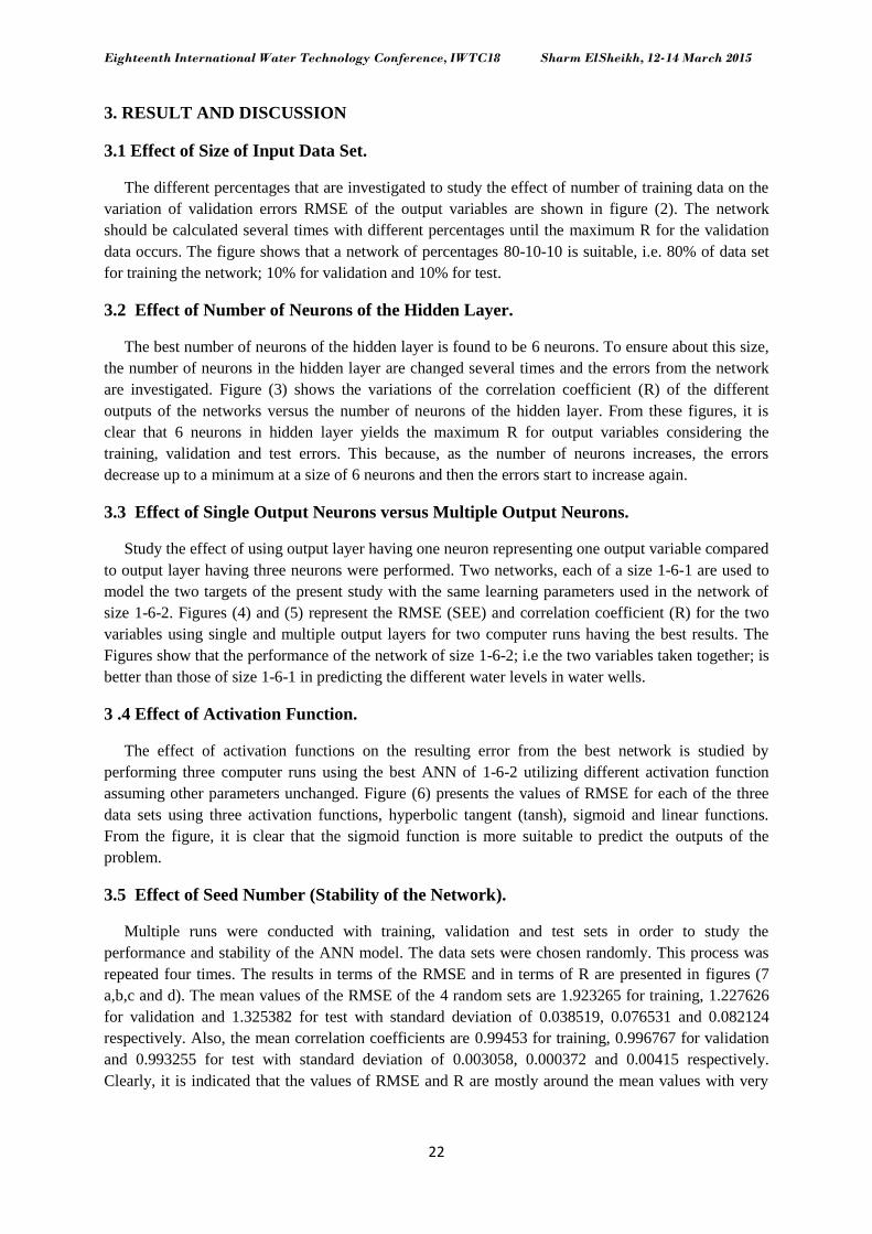
3. RESULT AND DISCUSSION

3.1 Effect of Size of Input Data Set.

The different percentages that are investigated to study the effect of number of training data on the

variation of validation errors RMSE of the output variables are shown in figure (2). The network

should be calculated several times with different percentages until the maximum R for the validation

data occurs. The figure shows that a network of percentages 80-10-10 is suitable, i.e. 80% of data set

for training the network; 10% for validation and 10% for test.

3.2 Effect of Number of Neurons of the Hidden Layer.

The best number of neurons of the hidden layer is found to be 6 neurons. To ensure about this size,

the number of neurons in the hidden layer are changed several times and the errors from the network

are investigated. Figure (3) shows the variations of the correlation coefficient (R) of the different

outputs of the networks versus the number of neurons of the hidden layer. From these figures, it is

clear that 6 neurons in hidden layer yields the maximum R for output variables considering the

training, validation and test errors. This because, as the number of neurons increases, the errors

decrease up to a minimum at a size of 6 neurons and then the errors start to increase again.

3.3 Effect of Single Output Neurons versus Multiple Output Neurons.

Study the effect of using output layer having one neuron representing one output variable compared

to output layer having three neurons were performed. Two networks, each of a size 1-6-1 are used to

model the two targets of the present study with the same learning parameters used in the network of

size 1-6-2. Figures (4) and (5) represent the RMSE (SEE) and correlation coefficient (R) for the two

variables using single and multiple output layers for two computer runs having the best results. The

Figures show that the performance of the network of size 1-6-2; i.e the two variables taken together; is

better than those of size 1-6-1 in predicting the different water levels in water wells.

3 .4 Effect of Activation Function.

The effect of activation functions on the resulting error from the best network is studied by

performing three computer runs using the best ANN of 1-6-2 utilizing different activation function

assuming other parameters unchanged. Figure (6) presents the values of RMSE for each of the three

data sets using three activation functions, hyperbolic tangent (tansh), sigmoid and linear functions.

From the figure, it is clear that the sigmoid function is more suitable to predict the outputs of the

problem.

3.5 Effect of Seed Number (Stability of the Network).

Multiple runs were conducted with training, validation and test sets in order to study the

performance and stability of the ANN model. The data sets were chosen randomly. This process was

repeated four times. The results in terms of the RMSE and in terms of R are presented in figures (7

a,b,c and d). The mean values of the RMSE of the 4 random sets are 1.923265 for training, 1.227626

for validation and 1.325382 for test with standard deviation of 0.038519, 0.076531 and 0.082124

respectively. Also, the mean correlation coefficients are 0.99453 for training, 0.996767 for validation

and 0.993255 for test with standard deviation of 0.003058, 0.000372 and 0.00415 respectively.

Clearly, it is indicated that the values of RMSE and R are mostly around the mean values with very


23

small standard deviation. This means that the developed ANN model is stable and hence the data are

consistent.

3.6 Outputs of Artificial Neural Networks

Output results of ANN compared to measured ones are presented in figures (4,5,6,and 7). The

figures show examples of the results of train, validation and test data for minimum and maximum

reading for the four testing wells. An excellent matching is observed in all cases indicating good

performance of the ANN model in predicting the ground water depth.

The correlation coefficients between the measured and predicted water depth using ANN model

are presented in table 3 for training, validation and test data sets. Also, as shown in figures 12 (a,b) a

very good matching between training, validation and test data for all 4 wells is observed which

indicates a good performance of the ANN model in predicting the ground water depth.

Table 3.: The values of correlation coefficients between the measured and predicted water depth for different wells

Well Name Data Value Data Type

Training Validation Test

5 – k – 60 Min. 0.932741 0.867173 0.965451

Max. 0.939142 0.878707 0.946914

5 – k – 83 Min. 0.966414 0.955318 0.971516

Max. 0.965854 0.956267 0.972403

5 – k – 84 Min. 0.992405 0.988784 0.988712

Max. 0.989395 0.992529 0.991950

5 – k – 87 Min. 0.988355 0.997312 0.996971

Max. 0.982605 0.997637 0.988779

3.7 Future Prediction

Fig (13) shows the relation between first, last and estimated readings after 20 years with minimum and

maximum water levels. The first readings were collected from about 32 years ago, while the last

readings were collected at recent years. Future prediction of well level of well 5-k-87 is about (-

119.00) while in wells 5-k-84, 5-k-83, 5-k-60 are (-80.00),(-160.00) and (-126.00) respectively. The

parentage of water level reduction after 20 years comparing with the reduction during the last 30 years

will be only 24 %, 29%, 17% and 23% for wells 5-k-87, 5-k-84, 5-k-83 and 5-k-60 respectively. It

means that the future reduction of the well water level in the coming 20 years will not exceed 30% of

the reduction done during the last 30 years.


24

4 SUMMARY AND CONCLUSION

A ground water level prediction has been conducted by using The Artificial Neural Networks

ANN. The ANN is used to develop a network of size 1-6-2 to predict the water level after 20 years.

Daily data of water level for period more than 30 years have been used for the prediction. The data

was collected from four wells located south of Riyadh city. A complete analysis of the 30 years data

has been conducted. Results of the prediction show that the reduction of the ground water level during

the coming 20 years will be no more than 30% of the reduction done through the last 30 years.

However, results still give warning to the local authorities in order to begin to conduct a reliable

strategy in order to reduce the future consumption of ground water.

ACKNOWLEDGMENT

This work was funded by the Deanship of scientific research in Salman bin Abdulaziz University,

KSA through a scientific research project under the title" Environmental assessment for the ground

water in agricultural area, El kharj",No (2/T/33).

REFERENCES

Abderrahman,W.(2005), "Groundwater Management for Sustainable Development of Urban and

Rural Areas in Extremely Arid Regions: A Case Study" Water Resources Development, Vol. 21, No.

3, 403–412, September 2005

ACSAD, 1999. Water resources division; objectives, functions and activities, The Arab Center for

the Studies of Arid Zones and Dry Lands, Damascus, Syria.

Al-Ibrahim, A.A. (1991), " Excessive Use of Groundwater Resources in Saudi Arabia: Impacts and

Policy Options" Ambio, Vol. 20, No. 1 (Feb., 1991),pp.34-37

Dibike, Y. B., and Abott, M. B. (1999). “Applications of Artificial Neural Networks to the

Simulation of a Two Dimensional Flow.” Journal of Hydraulic Research. Vol. 37, No. 4, pp. 435-446.

Dibike, Y. B., Minns, A., W. and Abott, M. B. (1999a). “Applications of Artificial Neural

Networks to the Generation of Wave Equations From Hydraulic Data.” Journal of Hydraulic Research.

Vol. 37, No. 1, pp. 81-97.

Dibike, Y. B., Solomatine, D., and Abott, M. B. (1999b). “On the Encapsulation of Numerical-

Hydraulic Models in Artificial Neural Network.” Journal of Hydraulic Research. Vol. 37, No. 2, pp.

147-162.

Elkiki, M. H. (2008a). “Prediction of Scour Parameters Downstream Skew Siphon Pipes Using

Artificial Neural Network Models”, Port-Said Engineering Research Journal, Faculty of Engineering,

Suez Canal University,Volume 12, No. 2,September, pp. 31-44.

Elkiki, M. H. (2008b). “Application of Artificial Neural Networks to predict the Drawdown Depth

Due to Ship Movement in Narrow Navigation Channels”, Port-Said Engineering Research Journal,

Faculty of Engineering, Suez Canal University,Volume 12, No. 2,September, pp. 45-59.

Kheireldin, K. A. (1999). “Neural Network Modeling for Clear Water Scour Around Bridge

Abutments.” Water Science, Scienific Journal of National Water Research Center, MWRI, El-Qanatir,

Egypt, Vol. 25, April, pp. 42-51.

Liriano, S. L., & Day, R. A. (2001). “Prediction of Scour Depth at Culvert Outlets Using Neural

Networks.” Journal of Hydroinformatics, Vol. 3, No. 4.


25

Mirdan, A. (2012). “Application of Artificial Neural Networks to Predict the Mean Velocity

Through Open Channel with Submerged Aquatic Weeds.” Scienific Journal of Civil Engineering,

Faculty of Engineering, Alazhar University, March 2012.

Negm, A. M. (2001). “Prediction of Hydraulic Parameters of Expanding Stilling Basins Using

Artificial Neural Networks.” Egyptian Journal For Engineering Sciences and Technology (EJEST),

Faculty of Engineering. Zagazig University, Zagazig, Egypt, Vol. 6, No. 1, pp. 1-24.

Negm, A. M., Saleh, O. K., and Ibrahim, A. A. (2002a). “Application of Artificial Neural Networks

to predict Flow Rates Below Vertical Sluice Gates.” Engineering Research Journal, Faculty of

Engineering, Helwan University, Mataria, Cairo, Egypt, Vol. 79, pp. 68-82.

Negm, A. M. (2002). “Generalized ANN Model For Discharge Below Silled-Sluice-Gate in

Prismatic Rectangular Channels.” Proc. Of 2nd Minia Int. Conf. For Advanced Trends in Engineering,

(MICATE 2002), Faculty of Engineering, El-Minia University, El-Minia, Egypt, April 7-9, pp. 284-

295.

Negm, A. M. & Shouman, M. A. (2002a). “Artificial Neural Network Model for Submerged

Hydraulic Jump Over Roughened Floor.” Proc. Of 2nd Minia Int. Conf. For Advanced Trends in

Engineering, (MICATE 2002), Faculty of Engineering, El-Minia University, El-Minia, Egypt, April 7-

9, pp. 319-330.

Negm, A. M., Abdel-Aal, G. M., Saleh, O. K., and Saudia, M. F. (2002b). “Prediction of Maximum

Scour Depth Downstream of Sudden Expanding Stilling Basins Using Artificial Neural Networks.”

Proc. Of 7th Alazhar Engineering Int. Conf. (AEIC 2003), April 7-10, Faculty of Engineering, Alazhar

University, Naser City, Cairo, Egypt.

Negm, A. M., Abdel-Aal, G. M., Elfiky, M. M., and Mohamed, Y. A. (2003). “Modeling of

Hydraulic Characteristics of Submerged Hydraulic Jump in Non-Prismatic Stilling Basins Using

ANN’s.” Proc. 1st Int. Conf. of Civil Eng. Science (ICCES 2003), Oct. 7-8, Assuit, Egypt.

Neural Connections (1998), “ANN software and Manuals.” Developed by SPSS/Reconition

Systems LTD.

Owais, T. M., Negm, A. M., Abdel-Aal, and Habib, A. A. (2003). “Prediction of The

Characteristics of Free Radial Hydraulic B-Jumps Formed at Sudden Drop Using ANN’s.” Proc. 7th

Int. Conf. on Water Technology (IWTC 2003), June 3-5, Cairo, Egypt, pp. 673-686.


26

Figure1. Wells Locations

0.97

0.975

0.98

0.985

0.99

0.995

1

50

-40

-10

50

-30

-20

50

-20

-30

50

-10

-40

60

-30

-10

60

-20

-20

60

-10

-30

70

-20

-10

70

-10

-20

80

-10

-10

Percentage of input data

R

Training

Validation

Test

b – min.

0.96

0.965

0.97

0.975

0.98

0.985

0.99

0.995

1

50

-40

-10

50

-30

-20

50

-20

-30

50

-10

-40

60

-30

-10

60

-20

-20

60

-10

-30

70

-20

-10

70

-10

-20

80

-10

-10

Percentage of input data

R

Training

Validation

Test

a - max.

Figure 2. Effect of percentages of input data on R of the training, validation and test data outputs for

max. and min. readings.


27

0.97

0.975

0.98

0.985

0.99

0.995

1

1.2.2 1.4.2 1.6.2 1.8.2 1.10.2

No. of neurons

R

Training

Validation

Test

b – min.

0.97

0.975

0.98

0.985

0.99

0.995

1

1.2.2 1.4.2 1.6.2 1.8.2 1.10.2

No. of neurons

RTraining

Validation

Test

a - max.

Figure 3. Effect of No. of neurons of hidden layer on R of the ANN outputs for max. and min. readings.

0

0.5

1

1.5

2

2.5

1.6.2 1.6.1

Output data set

RM

SE Training

Validation

Test

b – min.

0

0.5

1

1.5

2

2.5

1.6.2 1.6.1

Output data set

RM

SE Training

Validation

Test

a - max.

Figure 4. Effect of single and multiple output neurons on RMSE of the ANN outputs for max. and min. readings.

0.97

0.975

0.98

0.985

0.99

0.995

1

1.6.2 1.6.1

Output data set

R

Training

Validation

Test

b – min.

0.982

0.984

0.986

0.988

0.99

0.992

0.994

0.996

0.998

1

1.6.2 1.6.1

Output data set

R

Training

Validation

Test

a - max.

Figure 5. Effect of single and multiple output neurons on R of the ANN outputs for max. and min. readings.


28

0

0.5

1

1.5

2

2.5

3

3.5

Tanh Sigmoid Linear

Activation function

RM

SE Training

Validation

Test

b – min.

0

0.5

1

1.5

2

2.5

3

3.5

Tanh Sigmoid Linear

Activation function

RM

SE Training

Validation

Test

a - max.

Figure 6. Effect of activation function of hidden layer on RMSE of the ANN outputs for max/ and min. readings.

0

0.5

1

1.5

2

2.5

1 3 5 7

Seed No.

RM

SE Training

Validation

Test

b – min.

0

0.5

1

1.5

2

2.5

1 3 5 7

Seed No.

RM

SE Training

Validation

Test

a - max.

0.982

0.984

0.986

0.988

0.99

0.992

0.994

0.996

0.998

1 3 5 7

Seed No.

R

Training

Validation

Test

d – min.

0.995

0.9955

0.996

0.9965

0.997

0.9975

0.998

1 3 5 7

Seed No.

R

Training

Validation

Test

c - max.

Figure 7. Results of studying the stability of the network, (a,b) RMSE and (c,d) R of the ANN outputs for max.

and min. readings.


29

-110

-100

-90

-80

-70

-60

-50

-110 -100 -90 -80 -70 -60 -50

Measured water level (m)

Pre

dic

ted w

ater

lev

el (

m)

Validation data

Perfect fit

Figure 8. Examples of results of the predicted ANN model as compared with measured water level for different

(training, validation) data sets for min readings. (5-k-87)

-100

-90

-80

-70

-60

-50

-40

-30

-20

-100 -90 -80 -70 -60 -50 -40 -30 -20


Pre

dic

ted

wat

er lev

el (

m)

Test data

Perfect fit

-100

-90

-80

-70

-60

-50

-40

-30

-20

-100 -90 -80 -70 -60 -50 -40 -30 -20


Pre

dic

ted w

ater

lev

el (

m)

Training data

Perfect fit

Figure 9. Examples of results of the predicted ANN model as compared with measured water level for different

(training, test ) data sets for max. readings. (5-k-84)

-150

-130

-110

-90

-70

-50

-30

-150 -130 -110 -90 -70 -50 -30


Pre

dic

ted

wat

er lev

el (

m)

Test data

Perfect fit

-150

-130

-110

-90

-70

-50

-30

-150 -130 -110 -90 -70 -50 -30


Pre

dic

ted

wat

er lev

el (

m)

Validation data

Perfect fit

Figure 10. Examples of results of the predicted ANN model as compared with measured water level

for different (validation, test ) data sets for min. readings. (5-k-83)

-120

-110

-100

-90

-80

-70

-60

-120 -110 -100 -90 -80 -70 -60


Pre

dic

ted

wat

er lev

el (

m)

Test data

Perfect fit

-120

-110

-100

-90

-80

-70

-60

-120 -110 -100 -90 -80 -70 -60


Pre

dic

ted

wat

er lev

el (

m)

Validation data

Perfect fit

Figure 11. examples of results of the predicted ANN model as compared with measured water level for different

(validation, test ) data sets for max. readings. (5-k-60)

-110

-100

-90

-80

-70

-60

-50

-110 -100 -90 -80 -70 -60 -50


Pre

dic

ted

wat

er lev

el (

m)

Training data

Perfect fit


30

0.8

0.82

0.84

0.86

0.88

0.9

0.92

0.94

0.96

0.98

1

5-k-87 5-k-84 5-k-83 5-k-60

Well name

R

Training

Validation

Test

a - For max. readings

0.8

0.82

0.84

0.86

0.88

0.9

0.92

0.94

0.96

0.98

1

5-k-87 5-k-84 5-k-83 5-k-60

Well name.

R

Training

Validation

Test

a - For min. readings

Figure 12. The value of R of the ANN outputs for the different well name for (a) min. and (b) max. readings.

Well name (5-k-87)

-140

-120

-100

-80

-60

-40

-20

0

Min. Max.

Min. and Max. water lavel

Wate

r le

vel

First Reading

Last Reading

Estimated Reading after 20

years

Well name (5-k-84)

-90

-80

-70

-60

-50

-40

-30

-20

-10

0

Min. Max.

Min. and Max. water lavels

Wate

r le

vel

First Reading

Last Reading

Estimated Readings after

20 years

Well name (5-k-83)

-180

-160

-140

-120

-100

-80

-60

-40

-20

0

Min. Max.


Wate

r le

vel

First Reading

Last Reading


20 years

Well name (5-k-60)

-140

-120

-100

-80

-60

-40

-20

0

Min. Max.


Wate

r le

vel

First Reading

Last Reading


20 years

Figure 13. The relation between first, last and estimated readings after 20 years with min. and max. water levels.

Prediction of Future Ground Water Elevation by Using Artificial Neural Network South of Riyadh Ksa

Documents

Transcript of Prediction of Future Ground Water Elevation by Using Artificial Neural Network South of Riyadh Ksa