Prediction of bacterial interactions in the human...
43
Detecting bacterial associations in the human microbiome 10 th October 2012 Bertinoro Computational Biology Karoline Faust Raes Lab (Bioinformatics and (Eco-)Systems Biology)
Transcript of Prediction of bacterial interactions in the human...

Detecting bacterial associations in the human microbiome
10th October 2012Bertinoro Computational Biology
Karoline FaustRaes Lab (Bioinformatics and (Eco-)Systems Biology)

Examples for microbial relationships
cross-feeding between bacterial symbionts of a marine worm (Woyke et al.)
sulfur oxidizer sulfate reducer
Gause (1934) “The Struggle for Existence”, Williams & Wilkins.Kolenbrander et al. (2002) “Communication among Oral Bacteria”, Microbiol. and Mol. Biol. Reviews 66, pp. 486-505.Woyke, T. et al. (2006) “Symbiotic insights through metagenomic analysis of a microbial consortium”, Nature 443, pp. 950-955.1
. In
tro
du
ctio
n
dental plaque formation (Kolenbrander et al.)
Amoeba proteus feeding on algaeBacteriophages infecting a bacterium
competition between two species of Paramecium (Gause)
algae bloom killing off other organisms
artist’s rendering of human skin bacteria

Diamond, J. (1975) “Assembly of species communities”, pp. 342-444 in “Ecology and evolution of communities” edited by Cody and Diamond, Harvard University Press.Horner-Devine M.C. et al. (2007) “A Comparison Of Taxon Co-Occurrence Patterns For Macro- And Microorganisms” Ecology 88, pp. 1345-1353.
• Jared Diamond suggested that competition between species could be seen from their presences/absences across habitats (checkerboard pattern)• checkerboard-like co-occurrence patterns have been found for micro-organisms as well (Horner-Devine et al.)
1. I
ntr
od
uct
ion
Detecting ecological relationships from presence/absence data

1. I
ntr
od
uct
ion
Co-occurrence analysis in a nut shell
co-occurrence/correlation
mutual exclusion (checker board)/anti-correlation

Reasons for association
Adapted from Lidicker, W.Z. (1979) “A Clarification of Interactions in Ecological Systems”, BioScience 29, pp. 475-477.1
. In
tro
du
ctio
n
ecological relationships niche overlap
prey/host (loss-win)
predator/parasite (win-loss)
mu
tual
ism
(w
in-w
in)
amensalism(loss-neutral)
com
pet
itio
n (l
oss
-lo
ss)
+ -+ 0
+ +
0 +
0 -
- +
- -
- 0
commensalism(win-neutral)
Why would two taxa consistently occur together or avoid each other across samples?
Hutchinson, G.E. (1957) “Concluding remarks”, Cold Spring Harbour Symposium on Quantitative Biology 22, pp. 415-427.

Inferring networks
• network inference: the problem of finding relationships between objects (genes, proteins, metabolites, species...) whose presence/absence or abundance was observed repeatedly
ABC
A
B
C
1. I
ntr
od
uct
ion

• task: obtain functional protein modules from co-occurrences of genes
Example for similarity-based network inference
Date, S.V. and Marcotte, E.M. (2003) “Discovery of uncharacterized cellular systems by genome-wide analysis of functional linkages”, Nature Biotechnology 21, pp. 1055-1062.
genes
gene
s
1. I
ntr
od
uct
ion
organisms
gen
es
undirected network
similarity matrix
phylogenetic profiles

• task: identify gene regulatory network from microarray data
Example for sparse regression-basednetwork inference
gen
es
time/conditions
for each gene, find the regulators of that gene among all other genes:do sparse regression (using regression trees) to select the subset of input genes that predicts best the behavior of the output gene
1. I
ntr
od
uct
ion
Huynh-Thu et al. (2010) “Inferring regulatory networks from expression data using tree-based methods”, PLoS one 5, e12776.
directed networkmicroarray data sparse regression
input genes output gene

2. G
oal
Goal: Infer network of microbial relationships
• several recent metagenomic data sets measure microbial abundance across a large number of samples
• network inference techniques can identify significant relationships between microorganisms from these data
• significant co-presence (co-occurrence of two microbes across samples) can be interpreted as niche overlap, mutualism, commensalism etc.
• significant mutual exclusion (avoidance of two microbes across samples) can be interpreted as alternative niche preference, competition, amensalism etc.

The Human Microbiome Project
• 18 body sites (15 sites in males)
• 242 healthy individuals sampled up to three times
• 5,177 samples 16S RNA-sequenced
• > 3.5 TB metagenomic sequences
• Metadata collected (sex, age, ethnicity, BMI, pulse, medication, smoking behavior, vaginal pH, etc.)
3. D
ata
The Human Microbiome Project Consortium (2012) “A framework for human microbiome research”, Nature 486, pp. 215-221.
distribution of phyla across human body sites, according to 16S sequencing

16S sequencing and processing3
. Dat
a
• 5,177 samples pyro-sequenced (454 GS FLX Titanium) in 4 different centers (for V1-V3, V3-V5 and V6-V9 regions of 16S rRNA)
• 16S rRNA sequencing benchmarked on mock communities of known composition
• raw 16S rRNA reads were processed with mothur and Qiime pipelines
• mothur assigned reads to ~730 phylotypes and to ~9,450 OTUs(operational taxonomic units) using the RDP (Ribosomal Database Project) phylogenetic tree
• likely mislabeled samples removed using a machine learning approach (Knights, 2010)
Human Microbiome Project Data Generation Working Group (2012) “Evaluation of 16S rDNA-Based Community Profiling for Human Microbiome Research” PLoS ONE 7(6) e39315.Schloss, P. et al. (2009) “Introducing mothur: Open-source, platform-independent, community-supported software for describing and comparing microbial communities.” Appl. Environ. Microbiol. 75, pp. 7537-7541.Jumpstart Consortium Human Microbiome Project Data Generation Working Group “Evaluation of 16S rDNA-based Community Profiling for Human Microbiome Research”, PLoS one 7, e39315.Cole, J.R. et al. (2009) “The Ribosomal Database Project: improved alignments and new tools for rRNA analysis”, Nucleic Acid Research 37, pp. D141-D145.Knights, R. et al. (2010) “Supervised classification of microbiota mitigates mislabeling errors.” ISME 5, pp. 570-573.

Network inference from HMP data -Overview
4. M
eth
od
s
joint work with Huttenhower lab
• apply network inference strategies to predict relationships between bacterial taxa from the 16S HMP V35 phylotype data set (genus level)
high abundance
low abundance
... (12,450 rows, taxa in body sites)
... (392 columns, subjects sampled multiple times)
count matrix
positive cross-body-site link
negative intra-body-site link
network
network inference

4. M
eth
od
sAssessing strength of relationships
between microorganisms
Pair-wise relationships (similarity)- Pearson correlation- Spearman correlation- Kullback-Leibler dissimilarity (KLD)- Bray Curtis dissimilarity (BC)
Complex relationships (sparse regression)- GLBM (generalized, linear boosted models) to predict a target taxon from a set of source taxa by regression- score: the goodness of fit (how well combined source taxa profiles predict target taxon profile)
source taxa
target taxonabundance profiles across samples
Fah Sathirapongsasuti and Curtis Huttenhower

4. M
eth
od
sComputing significance of
relationships I
observed score
Freq
uen
cy
• for each of the five methods (Pearson, Spearman, Kullback-Leibler, Bray Curtis, GLBM), compute permutation and bootstrap edge scores
Freq
uen
cy
observed score
bootstrap distribution of method-specific edge score (confidence interval) permutation (null) distribution of method-
specific edge score
5 scores per edge, for each score:

4. M
eth
od
s
Fusobacteriales versus Streptococcaceae in buccalmucosa (Pearson)
Actinobacteria versus Bacteroidetes in subgingivalplaque (Spearman)
bootstrap distribution
renormalized permutation distribution
significantnot significant
score score
Edge- and method-specific p-value is computed with a Z-test (p-value of the null distribution mean given the bootstrap distribution, assuming normality for the bootstrap distribution)
Computing significance of relationships II

4. M
eth
od
sNetwork building
• merge method-specific p-values using Sime’s method
• apply Benjamini-Hochberg Yekutieli False Discovery Rate correction on merged p-values
• after correction, remove all p-values above the threshold (set to 0.05)
• represent remaining relationships as a network
p-value merge
multiple-testing correction
Pearson
Spearman
KLD
multigraph graph

• technical errors/differences in processing lead to different total abundances across samples
• sample-wise normalization necessary (i.e. division of abundances in a sample by this sample’s total abundance sum)
• absolute abundances are converted into proportions
4. M
eth
od
sProblem: Data normalization and
compositionality
taxa with the same abundance in two samples may represent different proportions

• Pearson and Spearman can be severely distorted, because they consider “absolute” values
• measures based on ratios or log-ratios (KLD, BC) are not affected by data compositionality, since the ratio between two abundances in the same sample is not changed by the normalization
Problem: Data normalization and compositionality
4. M
eth
od
s
Aitchison J (1982) “The Statistical Analysis of Compositional Data.” Journal of the Royal Statistical Society Series B (Methodological) 44, pp. 139-177.

Data normalization and compositionality -Example
4. M
eth
od
s
R1 R2 D
R1 1 -0.24 -0.69
R2 1 0.31
D 1
R1 R2 D
R1 1 -0.32 -0.73
R2 1 -0.41
D 1
DR1R2
Pearson correlation
raw data normalized data

• Permutation test: removes correlation, but also any bias due to compositionality• Permutation with renormalization: for each pair of taxa, permute their abundances and then normalize the matrix (body-site-wise)
4. M
eth
od
sAdjust null distribution to mitigate the
compositionality bias
shuffle selected taxon pair
renormalize matrixcompute random score for taxon pair on shuffled, renormalized abundances
FahSathirapong-sasuti
all taxa in one body site

Renormalization mitigates compositionality bias4
. Met
ho
ds
true correlation between b1 and b3 spurious correlation between b2 and b4 introduced by normalization
bootstrap distribution meanrenormalized permutation distribution mean
b1-b3 b2-b4
raw data normalized data
significant not significant
FahSathirapong-sasuti

Methodology overview4
. Met
ho
ds

Network inferred for HMP 16S phylotypes
Node color code
Anterior nares
Buccal mucosaHard palateKeratinized gingivaPalatine tonsilsSalivaSubgingival plaqueSupragingival plaqueThroatTongue dorsum
Left retroauricular creaseRight retroauricuar crease
Left antecubital fossaRight antecubital fossa
Stool
Mid vaginaPosterior fornixVaginal introitus
Edge color code
positive
negative
Nodes: body-site-specific phylotypes(e.g. Ruminococcaceae in Stool)Edges: significant score between body-site-specific phylotypes
• most edges connect phylotypes within the same body area (e.g. vagina), but some edges link phylotypes across body areas (network is modular)
5. R
esu
lts

5. R
esu
lts
HMP 16S Network - composition
EpsilonproteobacteriaFusobacteriaGammaproteobacteriaBetaproteobacteriaActinobacteriaBacteroidiaBacilliClostridiaAbove class-level
AlphaproteobacteriaLentisphaeriaVerrucomicrobiaeSynergistiaMollicutesNegativicutesErysipelotrichiSpriochaetesFlavobacteria
Posterior fornixMid vaginaRight antecubital fossaLeft antecubital fossaRight retroauricuar creaseVaginal introitusLeft retroauricular creaseKeratinized gingivaAnterior naresStool
Buccal mucosaThroatSubgingival plaquePalatine tonsilsSupragingival plaqueHard palateSalivaTongue dorsum
Body-site-specific node proportions
Class-specific node proportions
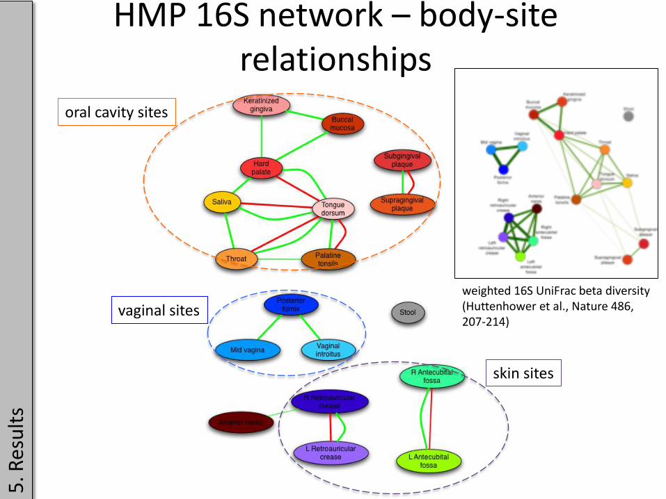
HMP 16S network – body-site relationships
oral cavity sites
vaginal sites
skin sites
5. R
esu
lts
weighted 16S UniFrac beta diversity (Huttenhower et al., Nature 486, 207-214)

5. R
esu
lts
HMP 16S network – class relationships

5. R
esu
lts
HMP 16S network analysis

5. R
esu
lts
HMP 16S network functional analysis
FahSathirapongsasutiand Nicola Segata

5. R
esu
lts
Vaginal sub-network of HMP 16S network
• Ravel et al. (2011): 5 vaginal community types identified
• 4 (I, II, III and V) of these dominated by Lactobacillus species
• 1 (IV) is diverse and contains members of Actinobacteria, Bacteroidetes and other phyla
• exclusion between Prevotellaceae(Bacteroidetes) and Lactobacillaceae as well as co-occurrence of anaerobic taxa (Finegoldia, Dialister, Peptoniphilus, Prevotellaceae), which are members of community IV
Ravel, J. et al. (2011) “Vaginal microbiome of reproductive-age women”, PNAS, vol. 108, pp. 4680-4687.
taxonomic levels shown: genus, family and class

5. R
esu
lts
Stool sub-network of HMP 16S network
• Arumugam et al. (2011): three different gut communities identified
• driven by: Prevotella, Bacteroides (both Bacteroidetes) and Ruminococcus(Firmicutes)
• Ruminococcaceae and Bacteroides as well as Prevotellaceae and Bacteroidesexclude each other in the stool sub-network
Arumugam, M., Raes, J. et al. (2011) “Enterotypes of the human gut microbiome”, Nature 473, pp. 174-180.
taxonomic levels shown: genus, family and class

Supragingival plaque sub-network of HMP 16S network
gingivadental plaque
- negative relationship between early colonizers of the tooth surface (Streptococcaceae) and intermediate colonizers (Fusobacterium)- positive relationships between late colonizers (Selenomonas, Tannerella)
5. R
esu
lts
Kolenbrander, P.E. et al. (2010) “Oral multispecies biofilm development and the key role of cell-cell distance”,Nature Reviews Microbiology 8, pp. 471-480.
taxonomic levels shown: genus

Conclusions
• few cross-body-area relationships: different body areas harbor distinct microbiota
• body sites can be grouped based on cross-links between their microbiota): oral, skin and vaginal sites form separate clusters, airways and stool separated from the oral cavity: clusters can be interpreted as different microbial niches
• alternative microbial communities observed in the vagina and the gut detected
• stages of dental plaque formation captured
• closely related microbes tend to co-occur in body sites with similar conditions
• negative relationships occur between more distantly related microbes
6. C
on
clu
sio
ns
Sathirapongsasuti*, Faust* et al. (2012) “Microbial Co-occurrence Relationships in the Human Microbiome”, PLoSComputational Biology 8 (7) e1002606.

CoNet – Similarity-based network inference with multiple measures
7. T
oo
l
Cytoscape main window

CoNet – Features7
. To
ol
• runs as Cytoscape plugin or on command line
• allows combining several measures, either in a multigraph or by merging their scores or p-values
• supports abundance as well as for presence/absence matrices
• implements various randomization and multiple test correction routines
• integrates external network inference packages, e.g. minet(mutual information based network inference) and apriori(association rule mining algorithm)
• plots score distributions
• offers preprocessing, missing value treatment, grouping rows
• settings loading/saving
• well documented (manual, tutorials, FAQ)
http://systemsbiology.vub.ac.be/conet

Outlook
• Dynamic network inference to decipher relationships among microorganisms in recent metagenomic time series data
image taken from Gajer et al. (2012) Sci. Transl. Med 4, 132ra52

Acknowledgement
Curtis Huttenhower
HMP Consortium for data access
Bioinformatics and (Eco-)Systems Biology (BSB) lab
Jeroen Raes
...and Dirk Gevers, Jacques Izard, Alvin Lo and Dominique Maes
Fah Sathirapongsasuti
Funding
Nicola Segata

• raw 16S rRNA reads were processed by Pat Schloss with his mothurpipeline
• processing steps included sequence trimming (primers and barcodes removal), filtering (of ambiguous bases, homo-polymers and redundant sequences) and chimera removal (with ChimeraSlayer)
• mothur assigned reads to ~730 phylotypes using the Ribosomal Database Project (RDP) reference 16S rRNA sequences and the RDP phylogenetic tree
• mothur also assigned reads to ~9,450 OTUs (operational taxonomic units), by first clustering reads based on alignments and then assigning a consensus taxonomy to the groups using the RDP phylogenetic tree and reference sequences
• likely mislabeled samples were detected by Dirk Gevers using a machine learning approach (Knights, 2010)
Bacterial abundances from 16S reads
Schloss, P. et al. (2009) “Introducing mothur: Open-source, platform-independent, community-supported software for describing and comparing microbial communities.” Appl. Environ. Microbiol., vol. 75, pp. 7537-7541Cole, J.R. et al. (2009) “The Ribosomal Database Project: improved alignments and new tools for rRNA analysis”, Nucleic Acid Research, vol. 37, pp. D141-D145Knights, R. et al. (2010) “Supervised classification of microbiota mitigates mislabeling errors.” ISME, vol. 5, pp. 570-573A
pp
end
ix

Selection of measuresExperiment: Select 1,000 top-ranked and 1,000 bottom-ranked measure-specific edges in Houston data subset
Jaccard similarity heat map (Ward clustering) based on edge overlapA
pp
end
ix

Definition of measures
d(x,y) x i y i 2
d(x,y) x i logx i
y i
y i log
y i
x i
d(x,y) log( x i) log( y i) 2
Hellinger(x and y each sum up to 1)
Kullback-Leibler(x and y each sum up to 1)
Logged Euclidean
Require pseudo-counts or smoothing because log(0) = -Inf
d(x,y) xi yi 2
Euclidean distance
Bray Curtis (Steinhaus is the corresponding similarity)
d(x,y) 12 min(xi,yi)
xi yi
Recommended for compositional data (absolute values are not of interest)
Recommended for taxon abundance data
Bray-Curtis dissimilarity is computed on row-wise normalized data (i.e. x and yeach sum up to 1)
Sup
ple
men
t
Hellinger distance and Kullback-Leiblerdivergence are mathematically related measures.

d(x,y) x i x y i y
x i x 2
y i y 2
d(x,y) 16 di
2n n2 1
,di x i y i(ranks)
For Pearson, vectors x and yare standardized (subtraction of mean, division by standard deviation) and for Spearman, ranks are considered, so vector-wise standardization is not necessary for either of these measures.
d(x,y) var(log(xi
yi
))
Pearson
Spearman
Variance of log-ratios
Variance of log-ratios, conceived for compositional data
Definition of measures continued
d(x,y) 1e d (x,y)
Aitchison proposed a scaling between 0 and 1, where 1 corresponds to maximal similarity:
Require pseudo-counts or smoothing because log(0) = -Inf
Ap
pen
dix

Generalized Boosted linear models (GBLM)
xtt, ts x tt, ts tt, ts, st, ssxst, ssst
Multiple regression: more than one source taxon may predict the target taxon’s abundance Boosting: a form of sparse regression (coefficients with small contributions are set to zero)
In practice, all source taxa of a body site are considered to predict the abundance of a target taxon in the same or another body site. Then, the optimal sub-set of source taxa is selected by boosting (sparsity enforcement).
xtt,ts = target taxon at target sitexst,ss= source taxon at source siteβ = coefficients (interaction strengths)
Ap
pen
dix

Generalized Boosted linear models (GBLM)
Regression scoring: adjusted R2 (AR)R2 = root mean square error between prediction and observation
AR2 1 (1R2 )n 1
n p 1
n = sample numberp = number of source taxa with non-zero coefficient
Scoring
Cross-validation
- boosting was carried out with three different iteration numbers (50, 100, 150)- the most accurate (according to AR2) selected among the three- 10-fold cross-validated and minimum AR2 retained as regression score
Prefiltering
- only source taxa correlating with target taxon with Spearman p-value < 0.05 considered (to enforce sparsity and avoid over-fitting)
Ap
pen
dix

Agreement between data and methodsA
pp
end
ix