Prediction of airborne sound and impact sound insulation ... · solid media. The model is ... The...
26
Prediction of airborne sound and impact sound insulation provided by single and multilayer systems using analytical expressions A. Tadeu * , A. Pereira, L. Godinho, J. Anto ´nio Department of Civil Engineering, Po ´ lo II of the University of Coimbra, Rua Luı ´ s Reis Santos, 3030-788 Coimbra, Portugal Received 25 May 2006; accepted 26 May 2006 Available online 17 July 2006 Abstract In this work, the authors use analytical solutions to assess the airborne sound and impact insu- lation provided by homogeneous partitions that are infinite along their plane. The algorithm uses Green’s functions, derived on the basis of previous work by the authors on the prediction of airborne sound insulation provided by single and double panels. The model is now extended to handle mul- tilayer systems, allowing the simulation of three-dimensional loads applied in both the acoustic and solid media. The model is validated against experimental results and compared with simplified expressions for single, double and triple panels. The results provided by the analytical model were found to provide a good agreement with the experimental results, except in the vicinity of the coincidence effect in the presence of thicker panels. The applicability of the proposed tool is then illustrated by analyzing the acoustic behavior pro- vided by single layers and by a suspended ceiling. Different variables are studied, such as the mass, the stiffness of the layers, the position and direction of the load within the elastic medium and the presence of porous material in the fluid layers. It was found that the model is able to simulate the acoustic phenomena involved in single and multilayer systems. Ó 2006 Elsevier Ltd. All rights reserved. Keywords: Airborne; Impact; Multilayer; Experimental 0003-682X/$ - see front matter Ó 2006 Elsevier Ltd. All rights reserved. doi:10.1016/j.apacoust.2006.05.012 * Corresponding author. Tel.: +351 239797201; fax: +351 239797190. E-mail address: [email protected] (A. Tadeu). Applied Acoustics 68 (2007) 17–42 www.elsevier.com/locate/apacoust
Transcript of Prediction of airborne sound and impact sound insulation ... · solid media. The model is ... The...

Applied Acoustics 68 (2007) 17–42
www.elsevier.com/locate/apacoust
Prediction of airborne sound and impactsound insulation provided by single and
multilayer systems using analytical expressions
A. Tadeu *, A. Pereira, L. Godinho, J. Antonio
Department of Civil Engineering, Polo II of the University of Coimbra, Rua Luıs Reis Santos,
3030-788 Coimbra, Portugal
Received 25 May 2006; accepted 26 May 2006Available online 17 July 2006
Abstract
In this work, the authors use analytical solutions to assess the airborne sound and impact insu-lation provided by homogeneous partitions that are infinite along their plane. The algorithm usesGreen’s functions, derived on the basis of previous work by the authors on the prediction of airbornesound insulation provided by single and double panels. The model is now extended to handle mul-tilayer systems, allowing the simulation of three-dimensional loads applied in both the acoustic andsolid media.
The model is validated against experimental results and compared with simplified expressions forsingle, double and triple panels. The results provided by the analytical model were found to provide agood agreement with the experimental results, except in the vicinity of the coincidence effect in thepresence of thicker panels.
The applicability of the proposed tool is then illustrated by analyzing the acoustic behavior pro-vided by single layers and by a suspended ceiling. Different variables are studied, such as the mass,the stiffness of the layers, the position and direction of the load within the elastic medium and thepresence of porous material in the fluid layers. It was found that the model is able to simulate theacoustic phenomena involved in single and multilayer systems.� 2006 Elsevier Ltd. All rights reserved.
Keywords: Airborne; Impact; Multilayer; Experimental
0003-682X/$ - see front matter � 2006 Elsevier Ltd. All rights reserved.
doi:10.1016/j.apacoust.2006.05.012
* Corresponding author. Tel.: +351 239797201; fax: +351 239797190.E-mail address: [email protected] (A. Tadeu).
18 A. Tadeu et al. / Applied Acoustics 68 (2007) 17–42
1. Introduction
The transmission of airborne sound energy through a single separation element dependson several variables, such as the frequency of sound incident on the element, the physicalproperties of the panel (mass, internal damping, elasticity modulus, Poisson’s ratio), theconnections with the surrounding structure and the vibration eigenmodes of the element.The prediction of the physical phenomena regarding wave propagation is quite complex,and this has led to several simplified models such as the theoretical Mass Law, whichassumes the element behaves like a group of infinite juxtaposed masses with independentdisplacement and null damping forces. Sewell [1] and Sharp [2] have proposed other sim-plified models for the frequencies below, in the vicinity of and above the coincidence effectto predict the airborne sound insulation provided by single panels.
But predicting the dynamic behavior of a multilayer system turns out to be more com-plex. Different simplified approaches have been proposed over the years. London [3] pre-dicted the sound insulation provided by double walls. In this model the double wall isexcited by plane waves at frequencies below the critical frequency and the mass is con-trolled to disregard panel resonance. The equation proposed by London takes intoaccount the effect of the resonance which occurs within the air gap. Beranek [4] later per-formed some mathematical manipulations in order to consider mass–air–mass resonance.The effect of an air gap filled with a porous sound-absorbing material has been simulatedby other authors [5].
Fringuellino et al. [6] calculated the transmission loss in multi-layered walls using a sim-plified approach based on the prior knowledge of the characteristic impedance of eachmaterial layer. Bolton et al. [7] described a theory for multi-dimensional wave propagationin elastic porous material, based on Biot’s theory, and used it to predict the airborne soundinsulation provided by foam-lined panels. When aluminium double-panel structures linedwith polyurethane foam were studied, the results provided by their models were found tobe good when compared with experimental results.
It is also important to predict the impact sound insulation provided by partitions at thedesign stage. The development of a prediction model has to take the excitation and thesound transmission system into account. In dwellings, the sources of annoyance can befootsteps or the impact of dropped objects. To evaluate the impact sound level experimen-tally, a standardized tapping machine, as described in the ISO standards, is used.Although this machine does not simulate real footsteps, the test results yield importantinformation concerning the dynamic behavior of the floor. Several authors have addressedthe problem of the excitation source, where the interaction at the interfaces between thehammer and the floor has to be considered. Cremer [8] has derived an impact source spec-trum caused by the tapping machine acting on homogeneous floors of high impedance. Heassumes that the impact is perfectly elastic and the results were proved to be satisfactoryfor several frequencies. Ver [9] derived a complete description of the force spectrum andimpact level provided by the tapping machine on hard surfaces. He also considered theimprovement in insulation provided by the use of elastic surface layers or by floating floorswith high-impedance surfaces.
Although the final response provided by the loads that act in the acoustic or in the elas-tic medium differs, the dynamic behavior of partitions may present similarities. Heckl et al.[10] found a relation between the airborne and impact sound insulation provided bypartitions.
A. Tadeu et al. / Applied Acoustics 68 (2007) 17–42 19
In this work, the authors propose an analytical model to assess the acoustic behavior ofsingle or multilayer partitions, infinite along their plane, dividing an infinite acoustic med-ium. The formulation of a set of analytical solutions for calculating the acoustic insulationprovided by single and double walls when submitted to incident pressure fields has beenpresented in earlier work [11–13]. This paper generalizes that model to solve structureswith an arbitrary number of elastic and acoustic layers, also allowing the application ofthree-dimensional impact loads. Thus, the proposed model can be used to predict theacoustic behavior of a broader range of acoustic systems than other models found inthe literature. In addition, it overcomes certain restrictions, such as the type and positionof the load, the number of layers and the assumption of the existence of incident planewaves. However, the model described here does not take into account the presence offlanking transmissions or sound bridges, since it assumes that the panels are uniform lay-ers of infinite extent, without mechanical fixings.
The present model defines a set of potentials in each layer that are combined so as toverify the boundary conditions and to predict the three-dimensional airborne and impactsound insulation (vertically and horizontally) provided by either a single structural layeror by a multilayer system. A point load is first represented by a summation of two-dimen-sional linear loads after the application of a Fourier transformation along the z direction(2.5D problem). Each linear load is in turn modeled as a superposition of plane sourcesfollowing the application of an additional Fourier transformation in the x direction.
The following section outlines the analytical 3D and 2.5D formulations used to predictairborne and impact sound insulation. The analytical formulation is then validated withexperimental results and compared with simplified expressions referenced in the literaturereview. For this, the airborne sound insulation provided by single and double panels is dis-cussed, after which the impact sound insulation provided by a single panel and by a float-ing layer system is examined. Finally, the applicability of the model is determined byassessing the acoustic behavior provided by a single structural layer excited by point loadsand by a suspended ceiling.
2. Analytical solution formulation
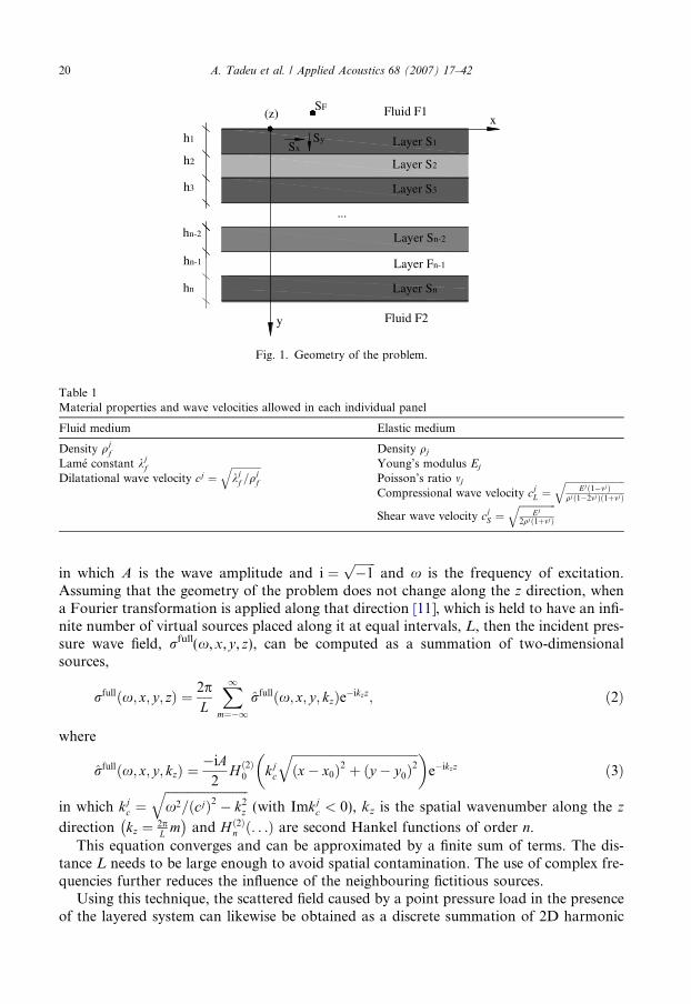
The analytical solutions are derived in the frequency domain for a multilayer system,infinite along the x and z directions, dividing an infinite acoustic medium (see Fig. 1). Thissystem can combine several elastic and fluid layers with different thicknesses hj
(j = 1,2, . . . ,n identifies the number of the layers).The material properties and the wave velocities allowed in each individual panel are
defined as in Table 1.
2.1. Formulation of the 3D problem
Consider the above-defined model to be excited by a point load, acting within one of itslayers. For the case of point pressure loads acting in a fluid layer at (x0,y0,z0), the incidentpressure wave field can be expressed by
rfullðx; x; y; zÞ ¼ Aeixcj cjt�
ffiffiffiffiffiffiffiffiffiffiffiffiffiffiffiffiffiffiffiffiffiffiffiffiffiffiffiffiffiffiffiffiffiffiffiffiðx�x0Þ2þðy�y0Þ2þðz�z0Þ2p� �
ffiffiffiffiffiffiffiffiffiffiffiffiffiffiffiffiffiffiffiffiffiffiffiffiffiffiffiffiffiffiffiffiffiffiffiffiffiffiffiffiffiffiffiffiffiffiffiffiffiffiffiffiffiffiffiffiffiffiffiffiffiffiffiffiðx� x0Þ2 þ ðy � y0Þ
2 þ ðz� z0Þ2q ð1Þ
h1
h2
h3
hn-2
...
xSF
SxSy
Fluid F1
Layer S1
Layer S2
Layer S3
Layer Sn-2
Layer Fn-1
Fluid F2
Layer Sn
hn-1
hn
(z)
y
Fig. 1. Geometry of the problem.
Table 1Material properties and wave velocities allowed in each individual panel
Fluid medium Elastic medium
Density qjf Density qj
Lame constant kjf Young’s modulus Ej
Dilatational wave velocity cj ¼ffiffiffiffiffiffiffiffiffiffiffiffikj
f =qjf
qPoisson’s ratio mj
Compressional wave velocity cjL ¼
ffiffiffiffiffiffiffiffiffiffiffiffiffiffiffiffiffiffiffiffiffiffiffiffiEjð1�mjÞ
qjð1�2mjÞð1þmjÞ
qShear wave velocity cj
S ¼ffiffiffiffiffiffiffiffiffiffiffiffiffiffiffi
Ej
2qjð1þmjÞ
q
20 A. Tadeu et al. / Applied Acoustics 68 (2007) 17–42
in which A is the wave amplitude and i ¼ffiffiffiffiffiffiffi�1p
and x is the frequency of excitation.Assuming that the geometry of the problem does not change along the z direction, whena Fourier transformation is applied along that direction [11], which is held to have an infi-nite number of virtual sources placed along it at equal intervals, L, then the incident pres-sure wave field, rfull(x,x,y,z), can be computed as a summation of two-dimensionalsources,
rfullðx; x; y; zÞ ¼ 2pL
X1m¼�1
rfullðx; x; y; kzÞe�ikzz; ð2Þ
where
rfullðx; x; y; kzÞ ¼�iA
2H ð2Þ0 kj
c
ffiffiffiffiffiffiffiffiffiffiffiffiffiffiffiffiffiffiffiffiffiffiffiffiffiffiffiffiffiffiffiffiffiffiffiffiffiffiffiffiffiðx� x0Þ2 þ ðy � y0Þ
2q� �
e�ikzz ð3Þ
in which kjc ¼
ffiffiffiffiffiffiffiffiffiffiffiffiffiffiffiffiffiffiffiffiffiffiffiffiffiffiffix2=ðcjÞ2 � k2
z
q(with Imkj
c < 0), kz is the spatial wavenumber along the z
direction kz ¼ 2pL m
� �and H ð2Þn ð. . .Þ are second Hankel functions of order n.
This equation converges and can be approximated by a finite sum of terms. The dis-tance L needs to be large enough to avoid spatial contamination. The use of complex fre-quencies further reduces the influence of the neighbouring fictitious sources.
Using this technique, the scattered field caused by a point pressure load in the presenceof the layered system can likewise be obtained as a discrete summation of 2D harmonic

A. Tadeu et al. / Applied Acoustics 68 (2007) 17–42 21
line loads, with different values of kz. This problem is often referred to in the literature as a2.5D problem, because the geometry is 2D and the source is 3D. The same procedure canbe applied to point loads acting in the x and y directions, in a solid medium, allowing thoseproblems to be solved as discrete summations of simpler 2.5D problems [11].
2.2. Formulation of the 2.5D problems
In this work, a generalization of the technique proposed by Tadeu et al. [11–13] is per-formed in order to handle multilayer systems and the application of impact loads. The ref-erenced authors derived a procedure to calculate the pressure field generated by a singlepanel, based on knowing the solid layer displacement potentials and the pressure poten-tials due to excitation by a spatially varying harmonic line load. In that method the poten-tials are written as a superposition of plane waves, by means of a discrete wavenumberrepresentation (after applying a Fourier transform in the x direction). The integrals ofthe expressions are then transformed into a discrete summation by assuming an infinitenumber of plane sources distributed along the x direction at equal intervals, Lx. It is thenpossible to compute the 2.5D response of the system as a summation of the effects of thedefined plane sources. After computing the solutions for a full sequence of 2.5D problemswith varying values of kz, the full 3D field generated by point loads can be determined as adiscrete summation of these 2.5D problems.
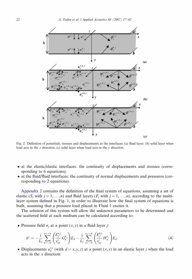
A multilayer system consists of a combination of solid and fluid layers. Thus, to achievethe solution provided by this system a set of dilatational and shear potentials generated ateach solid/fluid interface (interface a and b) must be defined. In a fluid layer (see Fig. 2a)the full description of the pressure field requires the knowledge of one dilatational poten-tial at each interface, while in the solid layer (see Fig. 2b and c) the displacement field iscomputed by making use of one dilatational and two shear displacement potentials at eachinterface, which depend on the orientation of the applied load. Table 2 lists the full set ofpotentials.
In the expressions listed in Table 2 the coefficients correspond to: Ea;jf ¼ e�imj
nf jy�ya;jj;
Eb;jf ¼ e�imj
nf jy�yb;jj; mjnf ¼
ffiffiffiffiffiffiffiffiffiffiffiffiffiffiffiffiffiffiffiffiffiffiffiffiffiffiffiffiffiffiffiffiðkj
pfÞ2 � k2
z � k2n
q, where Imðmj
nf Þ 6 0; kjpf¼ x=cj; ya,j and yb,j are
the y coordinates of the interfaces a and b which define the layer j using the coordinatesystem according to Fig. 1; Ea;j
b ¼ e�imjnjy�ya;jj; Eb;j
b ¼ e�imjnjy�yb;jj; Ea;j
c ¼ e�icjnjy�ya;jj;
Eb;jc ¼ e�icj
njy�yb;jj; cjn ¼
ffiffiffiffiffiffiffiffiffiffiffiffiffiffiffiffiffiffiffiffiffiffiffiffiffiffiffiffiffiffiðkj
sÞ2 � k2
z � k2n
q; kj
s ¼ x=cjS ; mj
n ¼ffiffiffiffiffiffiffiffiffiffiffiffiffiffiffiffiffiffiffiffiffiffiffiffiffiffiffiffiffiffiðkj
pÞ2 � k2
z � k2n
q, with
ImðmjnÞ 6 0; kj
p ¼ x=cjL; Ej
a ¼ 12qjx2Lx
; Ed ¼ e�iknðx�x0Þ; kn ¼ 2pLx
n and (x,y) defining the coordi-nates of a point inside the layer j. The coefficients Ax;Sj
n ; . . . ; F x;Sjn , Ay;Sj
n ; . . . ; F y;Sjn , GF j
n , andH F j
n are unknowns which are determined by solving a system of equations defined forthe specific multilayer problem. This system can be written by combining individual sys-tems of equations that are established for each layer. Each individual system of equationsis built by deriving the potentials in Table 2 in order to write the stresses and displacementsat the surfaces according to the layer and the source applied. The individual systems ofequations are fully described in Appendix 1. The final system of equations can then bewritten by combining these individual systems for each layer and prescribing the boundaryconditions:
� at the solid/fluid interfaces: the continuity of normal displacements and stresses andnull tangential stresses (corresponding to 4 equations);
,a jfη
,b jfη
a
b
h
,a jyu,a jυ
,b jyu,b jυ
x
y
z,a j
fφ
,b jfφ
a
b
h
,a jyu,a jσ
,b jyu,b jσ
x
y
z
(a)
a
b
h
, ,x a jη
, ,x b jη
, ,x a jy{
, ,x b jy{, ,x b j
z{
, ,x a jz{
, ,x b jyu
, ,x b jxu, ,x b j
zu
, ,x a jxu
, ,x a jyu
, ,x a jzu
, ,x b jyyυ
, ,x b jyzυ, ,x b j
yxυ
, ,x a jyzυ
, ,x a jyyυ
, ,x a jyxυ
xz
y
a
b
h
, ,x a jφ
, ,x b jφ
, ,x a jyψ
, ,x b jyψ, ,x b j
zψ
, ,x a jzψ
, ,x b jyu
, ,x b jxu, ,x b j
zu
, ,x a jxu
, ,x a jyu
, ,x a jzu
, ,x b jyyσ
, ,x b jyzυ, ,x b j
yxσ
, ,x a jyzσ
, ,x a jyyσ
, ,x a jyxσ
xz
y(b)
h
, ,y a jη
, ,y b jη
, ,y a jx{
, ,y b jx{, ,y b j
z{
, ,y a jz{
a
b, ,y b j
zu, ,y b j
yu
, ,y b jxu
, ,y a jyu
, ,y a jxu
, ,y a jzu
, ,y a jyzυ
, ,y a jyyυ
, ,y a jyxυ
, ,y b jyyυ
, ,y b jyzυ, ,y b j
yxυ
z x
y
h
, ,y a jφ
, ,y b jφ
, ,y a jxψ
, ,y b jxψ, ,y b j
zψ
, ,y a jzψ
a
b, ,y b j
zu, ,y b j
yu
, ,y b jxu
, ,y a jyu
, ,y a jxu
, ,y a jzu
, ,y a jyzσ
, ,y a jyyσ
, ,y a jyxσ
, ,y b jyyσ
, ,y b jyzσ, ,y b j
yxσ
z x
y(c)
Fig. 2. Definition of potentials, stresses and displacements at the interfaces: (a) fluid layer; (b) solid layer whenload acts in the x direction; (c) solid layer when load acts in the y direction.
22 A. Tadeu et al. / Applied Acoustics 68 (2007) 17–42
� at the elastic/elastic interfaces: the continuity of displacements and stresses (corre-sponding to 6 equations);� at the fluid/fluid interfaces: the continuity of normal displacements and pressures (cor-
responding to 2 equations).
Appendix 2 contains the definition of the final system of equations, assuming a set ofelastic (Sj with j = 1, . . . ,n) and fluid layers (Fj with j = 1, . . . ,n), according to the multi-layer system defined in Fig. 1, in order to illustrate how the final system of equations isbuilt, assuming that a pressure load placed in Fluid 1 excites it.
The solution of this system will allow the unknown parameters to be determined andthe scattered field at each medium can be calculated according to:
� Pressure field rj at a point (x,y) in a fluid layer j:
rj ¼ � i
Lx
Xn¼þN
n¼�N
Ea;jf
mjnf
GF jn
!Ed �
i
Lx
Xn¼þN
n¼�N
Eb;jf
mjnf
H F jn
!Ed : ð4Þ
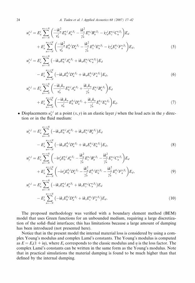
� Displacements ux;jd (with d = x,y,z) at a point (x,y) in an elastic layer j when the load
acts in the x direction:
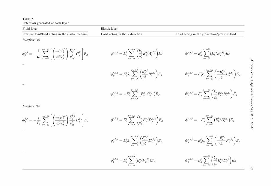
Table 2Potentials generated at each layer
Fluid layer Elastic layer
Pressure load/load acting in the elastic medium Load acting in the x direction Load acting in the y direction/pressure load
Interface (a)
/a;jf ¼ �
i
Lx
Xn¼þN
n¼�N
� cjð Þ2
x2kjf
!Ea;j
f
mjnf
GF jn
" #Ed /x;a;j ¼ Ei
a
Xn¼þN
n¼�N
kn
mjn
Ea;jb Ax;Sj
n
� �Ed /y;a;j ¼ Ej
a
Xn¼þN
n¼�N
ðEa;jb Ay;Sj
n ÞEd
–
wx;a;jy ¼ Ej
akz
Xn¼þN
n¼�N
Ea;jc
cjn
Bx;Sjn
� �Ed wy;a;j
x ¼ Ejakz
Xn¼þN
n¼�N
�Ea;jc
cjn
Cy;Sjn
� �Ed
–
wx;a;jz ¼ �Ej
a
Xn¼þN
n¼�N
Ea;jc Cx;Sj
n
� �Ed wy;a;j
z ¼ Eja
Xn¼þN
n¼�N
kn
cjn
Ea;jc By;Sj
n
� �Ed
Interface (b)
/b;jf ¼ �
i
Lx
Xn¼þN
n¼�N
�ðcjÞ2
x2kjf
!Eb;j
f
mjnf
H F jn
" #Ed /x;b;j ¼ Ej
a
Xn¼þN
n¼�N
kn
mjn
Eb;jb Dx;Sj
n
� �Ed /y;b;j ¼ �Ej
a
Xn¼þN
n¼�N
Eb;jb Dy;Sj
n
� �Ed
–
wx;b;jy ¼ Ej
akz
Xn¼þN
n¼�N
Eb;jc
cjn
Ex;Sjn
� �Ed wy;b;j
x ¼ Ejakz
Xn¼þN
n¼�N
�Eb;jc
cjn
F y;Sjn
� �Ed
–
wx;b;jz ¼ Ej
a
Xn¼þN
n¼�N
ðEb;jc F x;Sj
n ÞEd wy;b;jz ¼ Ej
a
Xn¼þN
n¼�N
kn
cjn
Eb;jc Ey;j
n
� �Ed
A.
Ta
deu
eta
l./
Ap
plied
Aco
ustics
68
(2
00
7)
17
–4
223
24 A. Tadeu et al. / Applied Acoustics 68 (2007) 17–42
ux;jx ¼ Ej
a
Xn¼þN
n¼�N
�ik2n
mjn
Ea;jb Ax;Sj
n � ik2z
cjn
Ea;jc Bx;Sj
n � icjnEa;j
c Cx;Sjn
� �Ed
þ Eja
Xn¼þN
n¼�N
�ik2n
mjn
Eb;jb Dx;Sj
n � ik2z
cjn
Eb;jc Ex;Sj
n � icjnEb;j
c F x;Sjn
� �Ed ; ð5Þ
ux;jy ¼ Ej
a
Xn¼þN
n¼�N
�iknEa;jb Ax;Sj
n þ iknEa;jc Cx;Sj
n
� �Ed
� Eja
Xn¼þN
n¼�N
�iknEb;jb Dx;Sj
n þ iknEb;jc F x;Sj
n
� �Ed ; ð6Þ
ux;jz ¼ Ej
a
Xn¼þN
n¼�N
�ikzkn
mjn
Ea;jb Ax;Sj
n þ ikzkn
cjn
Ea;jc Bx;Sj
n
� �Ed
þ Eja
Xn¼þN
n¼�N
�ikzkn
mjn
Eb;jb Dx;Sj
n þ ikzkn
cjn
Eb;jc Ex;Sj
n
� �Ed : ð7Þ
� Displacements uy;jd at a point (x,y) in an elastic layer j when the load acts in the y direc-
tion or in the fluid medium:
uy;jx ¼ Ej
a
Xn¼þN
n¼�N
�iknEa;jb Ay;Sj
n þ iknEa;jc By;Sj
n
� �Ed
� Eja
Xn¼þN
n¼�N
�iknEb;jb Dy;Sj
n þ iknEb;jc Ey;Sj
n
� �Ed ; ð8Þ
uy;jy ¼ Ej
a
Xn¼þN
n¼�N
�imjnEa;j
b Ay;Sjn � ik2
n
cjn
Ea;jc By;Sj
n � ik2z
cjn
Ea;jc Cy;Sj
n
� �Ed
þ Eja
Xn¼þN
n¼�N
�imjnEb;j
b Dy;Sjn � ik2
n
cjn
Eb;jc Ey;Sj
n � ik2z
cjn
Eb;jc F y;Sj
n
� �Ed ; ð9Þ
uy;jz ¼ Ej
a
Xn¼þN
n¼�N
�ikzEa;jb Ay;Sj
n þ ikzEa;jc Cy;Sj
n
� �Ed
� Eja
Xn¼þN
n¼�N
�ikzEb;jb Dy;Sj
n þ ikzEb;jc F y;Sj
n
� �Ed : ð10Þ
The proposed methodology was verified with a boundary element method (BEM)model that uses Green functions for an unbounded medium, requiring a large discretiza-tion of the solid–fluid interfaces; this has limitations because a large amount of dampinghas been introduced (not presented here).
Notice that in the present model the internal material loss is considered by using a com-plex Young’s modulus and complex Lame’s constants. The Young’s modulus is computedas E = Er(1 + ig), where Er corresponds to the classic modulus and g is the loss factor. Thecomplex Lame’s constants can be written in the same form as the Young’s modulus. Notethat in practical simulations the material damping is found to be much higher than thatdefined by the internal damping.
A. Tadeu et al. / Applied Acoustics 68 (2007) 17–42 25
3. Validation of the analytical model
In this section the analytical model is validated by comparing the responses againstexperimental results and simplified expressions. First the airborne sound insulation pro-vided by single- and double-layered partitions is analyzed. Then the impact sound insula-tion provided by a single panel and a concrete screed floating system is discussed.
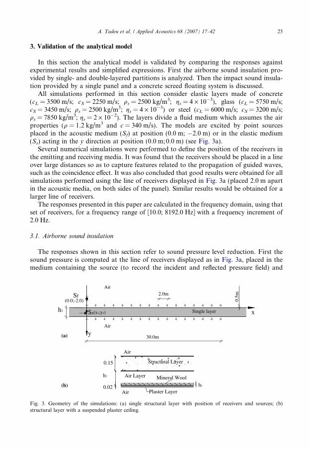
All simulations performed in this section consider elastic layers made of concrete(cL = 3500 m/s; cS = 2250 m/s; qs = 2500 kg/m3; gs = 4 · 10�3), glass (cL = 5750 m/s;cS = 3450 m/s; qs = 2500 kg/m3; gs = 4 · 10�3) or steel (cL = 6000 m/s; cS = 3200 m/s;qs = 7850 kg/m3; gs = 2 · 10�2). The layers divide a fluid medium which assumes the airproperties (q = 1.2 kg/m3 and c = 340 m/s). The models are excited by point sourcesplaced in the acoustic medium (Sf) at position (0.0 m; �2.0 m) or in the elastic medium(Ss) acting in the y direction at position (0.0 m; 0.0 m) (see Fig. 3a).
Several numerical simulations were performed to define the position of the receivers inthe emitting and receiving media. It was found that the receivers should be placed in a lineover large distances so as to capture features related to the propagation of guided waves,such as the coincidence effect. It was also concluded that good results were obtained for allsimulations performed using the line of receivers displayed in Fig. 3a (placed 2.0 m apartin the acoustic media, on both sides of the panel). Similar results would be obtained for alarger line of receivers.
The responses presented in this paper are calculated in the frequency domain, using thatset of receivers, for a frequency range of [10.0; 8192.0 Hz] with a frequency increment of2.0 Hz.
3.1. Airborne sound insulation
The responses shown in this section refer to sound pressure level reduction. First thesound pressure is computed at the line of receivers displayed as in Fig. 3a, placed in themedium containing the source (to record the incident and reflected pressure field) and
y
x
2.0m
0.5mSf
Ssh1
Air
Air
Single layer(xs;ys)
(0.0;-2.0)
30.0m(a)
0.15
h
0.02
Structural Layer
Air Layer
Air
Air Plaster Layer
Mineral Woolh3
2
(b)
Fig. 3. Geometry of the simulations: (a) single structural layer with position of receivers and sources; (b)structural layer with a suspended plaster ceiling.
26 A. Tadeu et al. / Applied Acoustics 68 (2007) 17–42
in the receiving medium. Then the sound pressure level reduction is calculated by means ofthe difference between the ratio of the average of the sound pressure squared to the squareof the reference sound pressure in the medium containing the source and in the receivingmedium on a dB scale.
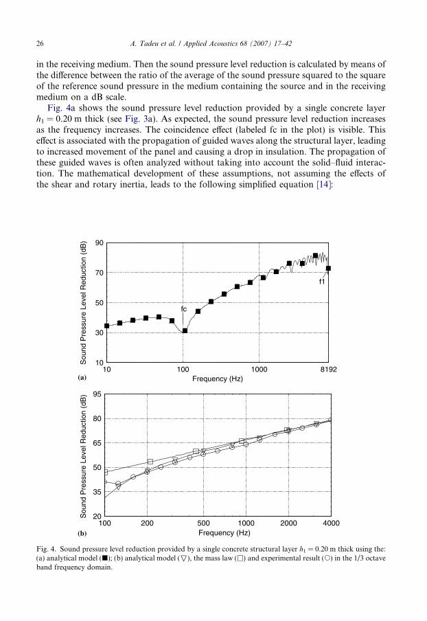
Fig. 4a shows the sound pressure level reduction provided by a single concrete layerh1 = 0.20 m thick (see Fig. 3a). As expected, the sound pressure level reduction increasesas the frequency increases. The coincidence effect (labeled fc in the plot) is visible. Thiseffect is associated with the propagation of guided waves along the structural layer, leadingto increased movement of the panel and causing a drop in insulation. The propagation ofthese guided waves is often analyzed without taking into account the solid–fluid interac-tion. The mathematical development of these assumptions, not assuming the effects ofthe shear and rotary inertia, leads to the following simplified equation [14]:
10
30
50
70
90
10 100 1000 8192
f1
fc
Frequency (Hz)
Sou
nd P
ress
ure
Leve
l Red
uctio
n (d
B)
(a)
20
35
50
65
80
95
100 200 500 1000 2000 4000Frequency (Hz)
Sou
nd P
ress
ure
Leve
l Red
uctio
n (d
B)
(b)
Fig. 4. Sound pressure level reduction provided by a single concrete structural layer h1 = 0.20 m thick using the:(a) analytical model (j); (b) analytical model (O), the mass law (�) and experimental result (s) in the 1/3 octaveband frequency domain.
A. Tadeu et al. / Applied Acoustics 68 (2007) 17–42 27
x ¼ csin /
ffiffiffiffiffiffiffiffiffiqsh1
D
r; ð11Þ
where qs is the density of the material (kg/m3), h1 is the thickness of the panel (m);D ¼ h3
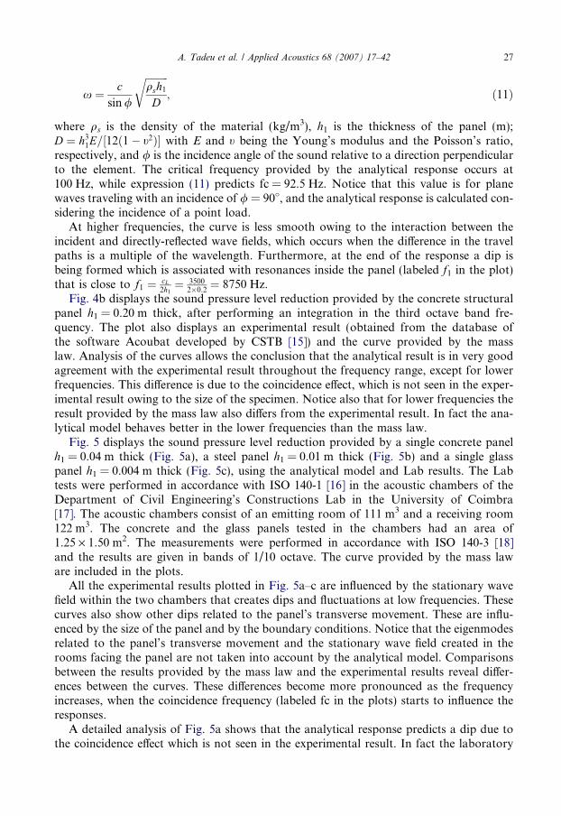
1E=½12ð1� t2Þ� with E and t being the Young’s modulus and the Poisson’s ratio,respectively, and / is the incidence angle of the sound relative to a direction perpendicularto the element. The critical frequency provided by the analytical response occurs at100 Hz, while expression (11) predicts fc = 92.5 Hz. Notice that this value is for planewaves traveling with an incidence of / = 90�, and the analytical response is calculated con-sidering the incidence of a point load.
At higher frequencies, the curve is less smooth owing to the interaction between theincident and directly-reflected wave fields, which occurs when the difference in the travelpaths is a multiple of the wavelength. Furthermore, at the end of the response a dip isbeing formed which is associated with resonances inside the panel (labeled f1 in the plot)that is close to f1 ¼ cL
2h1¼ 3500
2�0:2¼ 8750 Hz.
Fig. 4b displays the sound pressure level reduction provided by the concrete structuralpanel h1 = 0.20 m thick, after performing an integration in the third octave band fre-quency. The plot also displays an experimental result (obtained from the database ofthe software Acoubat developed by CSTB [15]) and the curve provided by the masslaw. Analysis of the curves allows the conclusion that the analytical result is in very goodagreement with the experimental result throughout the frequency range, except for lowerfrequencies. This difference is due to the coincidence effect, which is not seen in the exper-imental result owing to the size of the specimen. Notice also that for lower frequencies theresult provided by the mass law also differs from the experimental result. In fact the ana-lytical model behaves better in the lower frequencies than the mass law.
Fig. 5 displays the sound pressure level reduction provided by a single concrete panelh1 = 0.04 m thick (Fig. 5a), a steel panel h1 = 0.01 m thick (Fig. 5b) and a single glasspanel h1 = 0.004 m thick (Fig. 5c), using the analytical model and Lab results. The Labtests were performed in accordance with ISO 140-1 [16] in the acoustic chambers of theDepartment of Civil Engineering’s Constructions Lab in the University of Coimbra[17]. The acoustic chambers consist of an emitting room of 111 m3 and a receiving room122 m3. The concrete and the glass panels tested in the chambers had an area of1.25 · 1.50 m2. The measurements were performed in accordance with ISO 140-3 [18]and the results are given in bands of 1/10 octave. The curve provided by the mass laware included in the plots.
All the experimental results plotted in Fig. 5a–c are influenced by the stationary wavefield within the two chambers that creates dips and fluctuations at low frequencies. Thesecurves also show other dips related to the panel’s transverse movement. These are influ-enced by the size of the panel and by the boundary conditions. Notice that the eigenmodesrelated to the panel’s transverse movement and the stationary wave field created in therooms facing the panel are not taken into account by the analytical model. Comparisonsbetween the results provided by the mass law and the experimental results reveal differ-ences between the curves. These differences become more pronounced as the frequencyincreases, when the coincidence frequency (labeled fc in the plots) starts to influence theresponses.
A detailed analysis of Fig. 5a shows that the analytical response predicts a dip due tothe coincidence effect which is not seen in the experimental result. In fact the laboratory

0
20
40
60
80
100 100050 6000
fc
Frequency (Hz)
Sou
nd P
ress
ure
Leve
l Red
uctio
n (d
B)
(a)
0
20
40
60
100 100050 6000
fc
Frequency (Hz)
Sou
nd P
ress
ure
Leve
l Red
uctio
n (d
B)
(b)
0
10
20
30
40
50
100 100050 6000
fc
Frequency (Hz)
Sou
nd P
ress
ure
Leve
l Red
uctio
n (d
B)
(c)
Fig. 5. Sound pressure level reduction using the analytical model (s) vs experimental results (d) vs the mass law(h) provided by a: (a) single concrete layer h1 = 0.04 m thick; (b) single steel layer h1 = 0.01 m thick; (c) singleglass layer h1 = 0.004 m thick.
28 A. Tadeu et al. / Applied Acoustics 68 (2007) 17–42
A. Tadeu et al. / Applied Acoustics 68 (2007) 17–42 29
test used a panel with an area of 1.25 · 1.50 m2. The panel tested was not large enough forthis phenomenon to be seen in the experimental response. At higher frequencies bothcurves present a very good agreement. Analysis of Fig. 5b allows similar conclusions tobe drawn. When a glass panel is assumed (see Fig. 5c) the experimental curve exhibitsthe presence of the coincidence effect. Here the response provided by the analytical modelshows an excellent agreement, even in the vicinity of the coincidence effect.
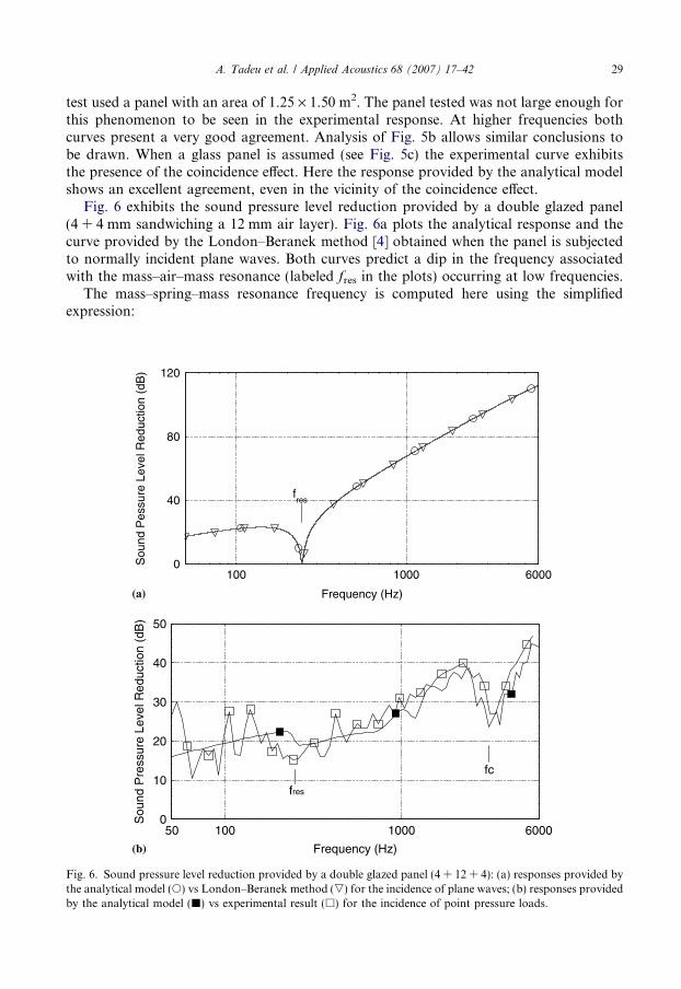
Fig. 6 exhibits the sound pressure level reduction provided by a double glazed panel(4 + 4 mm sandwiching a 12 mm air layer). Fig. 6a plots the analytical response and thecurve provided by the London–Beranek method [4] obtained when the panel is subjectedto normally incident plane waves. Both curves predict a dip in the frequency associatedwith the mass–air–mass resonance (labeled fres in the plots) occurring at low frequencies.
The mass–spring–mass resonance frequency is computed here using the simplifiedexpression:
0
40
80
120
100 1000 6000
fres
Frequency (Hz)
Sou
nd P
essu
re L
evel
Red
uctio
n (d
B)
(a)
(b)
0
10
20
30
40
50
100 100050 6000
fc
fres
Frequency (Hz)
Sou
nd P
ress
ure
Leve
l Red
uctio
n (d
B)
Fig. 6. Sound pressure level reduction provided by a double glazed panel (4 + 12 + 4): (a) responses provided bythe analytical model (s) vs London–Beranek method (,) for the incidence of plane waves; (b) responses providedby the analytical model (j) vs experimental result (h) for the incidence of point pressure loads.

30 A. Tadeu et al. / Applied Acoustics 68 (2007) 17–42
fres ¼1
2p
ffiffiffiffiffiffiffiffiffiffiffiffiffiffiffiffiffiffiffiffiffiffiffiffiffiffiffiK
1
m1
þ 1
m2
� �s; ð12Þ
where K ¼ c2qf
h2with c and qf being the dilatational wave velocity and the density of the air,
respectively; m1 and m2 are the mass of each layer (kg/m2) and h2 is the thickness of the airgap. The resonance of the mass–air–mass system predicted using expression (12) leads tofres = 244 Hz. This result is similar to that provided by the analytical model. Analysis ofthe figure reveals very good agreement between the analytical solution and the curve pro-vided by London–Beranek method.
Fig. 6b shows the analytical response provided by the double glazed panel when sub-jected to a point pressure load, and the experimental result obtained by testing a panelwith an area of 1.25 · 1.50 m2 [17]. All the results show dips associated with the mass–air–mass resonance and the coincidence effect. As before, the resonance effect inside theair layer is not visible as it occurs outside the frequency domain used in the analysis. Againthe analytical result tends to show a good agreement with the experimental solution,except at low frequencies, owing to the fluctuations related to the stationary field gener-ated in the emitting and receiving rooms of the chamber. Notice that the dip associatedwith the coincidence effect predicted by the analytical model is very similar with the exper-imental result.
The results presented above did not take into account the existence of flanking trans-mission through the side elements. In cases where this phenomenon may be relevant thesound pressure reduction will be lower than that found by the analytical model. In thesesituations, the contribution of flanking transmission can be calculated using the proceduredescribed in EN 12354-1 [19].
3.2. Impact sound pressure level
In this section the impact sound pressure level results provided by the analytical modeland by the experimental tests are discussed. The responses provided by the analyticalmodel are obtained by calculating the ratio of the average of the sound pressure squaredto the square of the reference sound pressure recorded at the receivers placed in the receiv-ing medium, as shown in Fig. 3a.
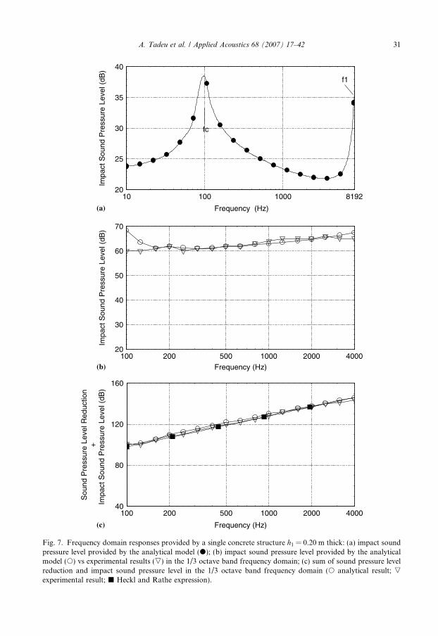
Fig. 7 displays the results provided by a single concrete layer h1 = 0.20 m thick. Fig. 7ashows the response provided by the analytical model simulating a theoretical impact froma standard tapping machine. The results show that the sound level increases in the vicinityof both the coincidence effect and the resonances inside the elastic layer (labeled as f1 in theplot).
Fig. 7b plots the analytical and experimental results provided by the concrete layerunder the action of a standard tapping machine (obtained from the software Acoubatdeveloped by CSTB [15]). In order to compare our results with the experimental curve,the amplitude of the impact load is defined in the frequency domain so as to model theresponse provided by a standard tapping machine. The frequency spectrum of the impactload is obtained from the approach followed by Cremer [8]. According to this author theimpact provided by the tapping machine (rate of the hammer strikes – 10 Hz) on a highimpedance structure, in the frequency domain, exhibits a constant amplitude of8.859 N. The results are shown in the 1/3 octave frequency bands. The two curves in
20
25
30
35
40
10 100 1000 8192
f1
fc
Frequency (Hz)
Impa
ct S
ound
Pre
ssur
e Le
vel (
dB)
(a)
20
30
40
50
60
70
100 200 500 1000 2000 4000
Frequency (Hz)
Frequency (Hz)
Impa
ct S
ound
Pre
ssur
e Le
vel (
dB)
(b)
40
80
120
160
100 200 500 1000 2000 4000
Sou
nd P
ress
ure
Leve
l Red
uctio
n+
Impa
ct S
ound
Pre
ssur
e Le
vel (
dB)
(c)
Fig. 7. Frequency domain responses provided by a single concrete structure h1 = 0.20 m thick: (a) impact soundpressure level provided by the analytical model (d); (b) impact sound pressure level provided by the analyticalmodel (s) vs experimental results (,) in the 1/3 octave band frequency domain; (c) sum of sound pressure levelreduction and impact sound pressure level in the 1/3 octave band frequency domain (s analytical result; ,
experimental result; j Heckl and Rathe expression).
A. Tadeu et al. / Applied Acoustics 68 (2007) 17–42 31
32 A. Tadeu et al. / Applied Acoustics 68 (2007) 17–42
the plot exhibit similar behavior, except at the lower frequencies. In fact the experimentalresponse provided by the concrete floors is not influenced by the coincidence effect that ispredicted by the analytical model.
The results provided by the analytical model are also compared with the simplifiedexpression achieved by Heckl et al. [10], modified for 1/3 octave frequency bands,
Ln þ R ¼ 38þ 30 logðfmÞ; ð13Þwhere fm is the third octave band center frequency in Hz; R is the sound transmission lossof an element, and Ln is the impact sound pressure level, defined as the sound level mea-sured in the receiving room when a standard tapping machine is operating. This expressionassumes that the coincidence frequency is low and the surface is hard and has high inputimpedance. According to the authors, this relation does not hold if there is a hole in theelement, which allows the waves produced by the pressure source and the impact soundwaves to travel along different path, or if the flanking transmission through the side wallsis dominant in relation to that occurring through the structural layer.
The sum of airborne and impact sound insulation is computed for the single concretelayer and integrations in the 1/3 octave band frequency are performed. Responses pro-vided by the analytical model, experimental results and expression (13) are plotted inFig. 7c. The results show that the two curves exhibit similar behavior. The good agreementthat is found between curves is related to the fact that the proposed model is based on theassumption that the panels are of infinite extent, meaning that the results do not accountfor flanking transmission.
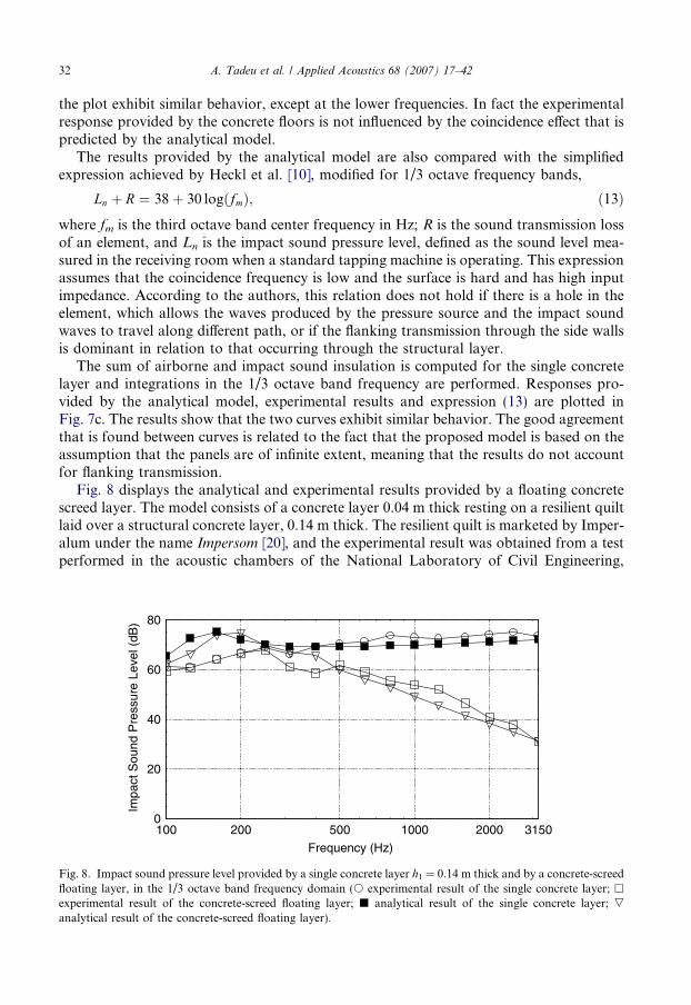
Fig. 8 displays the analytical and experimental results provided by a floating concretescreed layer. The model consists of a concrete layer 0.04 m thick resting on a resilient quiltlaid over a structural concrete layer, 0.14 m thick. The resilient quilt is marketed by Imper-alum under the name Impersom [20], and the experimental result was obtained from a testperformed in the acoustic chambers of the National Laboratory of Civil Engineering,
0
20
40
60
80
100 200 500 1000 2000 3150
Frequency (Hz)
Impa
ct S
ound
Pre
ssur
e Le
vel (
dB)
Fig. 8. Impact sound pressure level provided by a single concrete layer h1 = 0.14 m thick and by a concrete-screedfloating layer, in the 1/3 octave band frequency domain (s experimental result of the single concrete layer; h
experimental result of the concrete-screed floating layer; j analytical result of the single concrete layer; ,
analytical result of the concrete-screed floating layer).
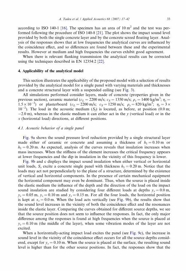
A. Tadeu et al. / Applied Acoustics 68 (2007) 17–42 33
according to ISO 140-1 [16]. The specimen has an area of 10 m2 and the test was per-formed following the procedure of ISO 140-8 [21]. The plot shows the impact sound levelprovided by both the single concrete layer and by the concrete screed floating layer. Anal-ysis of the responses shows that at low frequencies the analytical curves are influenced bythe coincidence effect, and so differences are found between these and the experimentalresults. However at medium and high frequencies the curves exhibit good agreement.
When there is relevant flanking transmission the analytical results can be correctedusing the techniques described in EN 12354:2 [22].
4. Applicability of the analytical model
This section illustrates the applicability of the proposed model with a selection of resultsprovided by the analytical model for a single panel with varying materials and thicknessesand a concrete structural layer with a suspended ceiling (see Fig. 3).
All simulations performed consider layers, made of concrete (properties given in theprevious section), ceramic material (cL = 2200 m/s; cS = 1350 m/s; qs = 1400 kg/m3; gs =1.5 · 10�2) or plasterboard (cL = 2200 m/s; cS = 1250 m/s; qs = 820 kg/m3; gs = 3 ·10�2). The load in the acoustic medium (Sf) is located, as before, at position (0.0 m;�2.0 m), whereas in the elastic medium it can either act in the y (vertical load) or in thex (horizontal load) directions, at different positions.
4.1. Acoustic behavior of a single panel
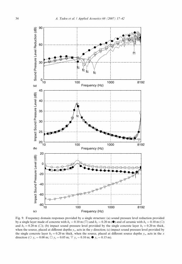
Fig. 9a shows the sound pressure level reduction provided by a single structural layermade either of ceramic or concrete and assuming a thickness of h1 = 0.10 m orh1 = 0.20 m. As expected, analysis of the curves reveals that insulation increases whenmass increases. When the stiffness of the element increases the critical frequency appearsat lower frequencies and the dip in insulation in the vicinity of this frequency is lower.
Fig. 9b and c displays the impact sound insulation when either vertical or horizontalunit loads, Ss excite a concrete single panel with thickness h1 = 0.20 m. Notice that theloads may act not perpendicularly to the plane of a structure, determined by the existenceof vertical and horizontal components. In the presence of certain mechanical equipmentthe horizontal component may even be dominant. Thus, when the source is placed insidethe elastic medium the influence of the depth and the direction of the load on the impactsound insulation are studied by considering four different loads at depths ys = 0.0 m,ys = 0.05 m, ys = 0.10 m and ys = 0.15 m. For all the four loads, the horizontal positionis kept at xs = 0.0 m. When the load acts vertically (see Fig. 9b), the results show thatthe sound level increases in the vicinity of both the coincidence effect and the resonancesinside the elastic layer. Comparing the curves obtained for different source depths, we seethat the source position does not seem to influence the responses. In fact, the only majordifference among the responses is found at high frequencies when the source is placed atys = 0.10 m (the middle of the layer), when some vibration modes of the layer are notexcited.
When a horizontally-acting impact load excites the panel (see Fig. 9c), the increase insound level in the vicinity of the coincidence effect occurs for all the source depths consid-ered, except for ys = 0.10 m. When the source is placed at the surface, the resulting soundlevel is higher than for the other source positions. In fact, the responses show that the
0
30
60
90
10 100 1000 8192Frequency (Hz)
Frequency (Hz)
Frequency (Hz)
Sou
nd P
ress
ure
Leve
l Red
uctio
n (d
B)
(a)
20
25
30
35
40
45
10 100 1000 8192
fc
Impa
ct S
ound
Pre
ssur
e Le
vel (
dB)
(b)
-80
-60
-40
-20
0
20
10 100 1000 8192
Impa
ct S
ound
Pre
ssur
e Le
vel (
dB)
(c)
fc
f1
fcfcfc
Fig. 9. Frequency domain responses provided by a single structure: (a) sound pressure level reduction providedby a single layer made of concrete with h1 = 0.10 m (,) and h1 = 0.20 m (d) and of ceramic with h1 = 0.10 m (s)and h1 = 0.20 m (h); (b) impact sound pressure level provided by the single concrete layer h1 = 0.20 m thick,when the source, placed at different depths ys, acts in the y direction; (c) impact sound pressure level provided bythe single concrete layer h1 = 0.20 m thick, when the source, placed at different source depths ys, acts in the x
direction (s ys = 0.00 m; h ys = 0.05 m; , ys = 0.10 m; d ys = 0.15 m).
34 A. Tadeu et al. / Applied Acoustics 68 (2007) 17–42
A. Tadeu et al. / Applied Acoustics 68 (2007) 17–42 35
sound level in the receiving space is highly influenced by the source depth. When the depthis ys = 0.10 m the influence of the propagating guided waves does not seem to be impor-tant and the impact insulation appears to be much lower than that obtained for the otherpositions. Moreover, sound level increases as frequency increases. Comparison with theresponses shown in Fig. 9b indicates that the contribution to impact sound insulationof the source acting horizontally is lower than when the load acts vertically. When the loadacts horizontally more energy travels along the panel and less is radiated into the receivingmedium.
4.2. Acoustic behavior of a concrete layer with a suspended ceiling
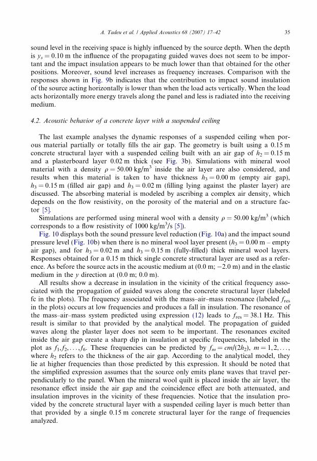
The last example analyses the dynamic responses of a suspended ceiling when por-ous material partially or totally fills the air gap. The geometry is built using a 0.15 mconcrete structural layer with a suspended ceiling built with an air gap of h2 = 0.15 mand a plasterboard layer 0.02 m thick (see Fig. 3b). Simulations with mineral woolmaterial with a density q = 50.00 kg/m3 inside the air layer are also considered, andresults when this material is taken to have thickness h3 = 0.00 m (empty air gap),h3 = 0.15 m (filled air gap) and h3 = 0.02 m (filling lying against the plaster layer) arediscussed. The absorbing material is modeled by ascribing a complex air density, whichdepends on the flow resistivity, on the porosity of the material and on a structure fac-tor [5].
Simulations are performed using mineral wool with a density q = 50.00 kg/m3 (whichcorresponds to a flow resistivity of 1000 kg/m3/s [5]).
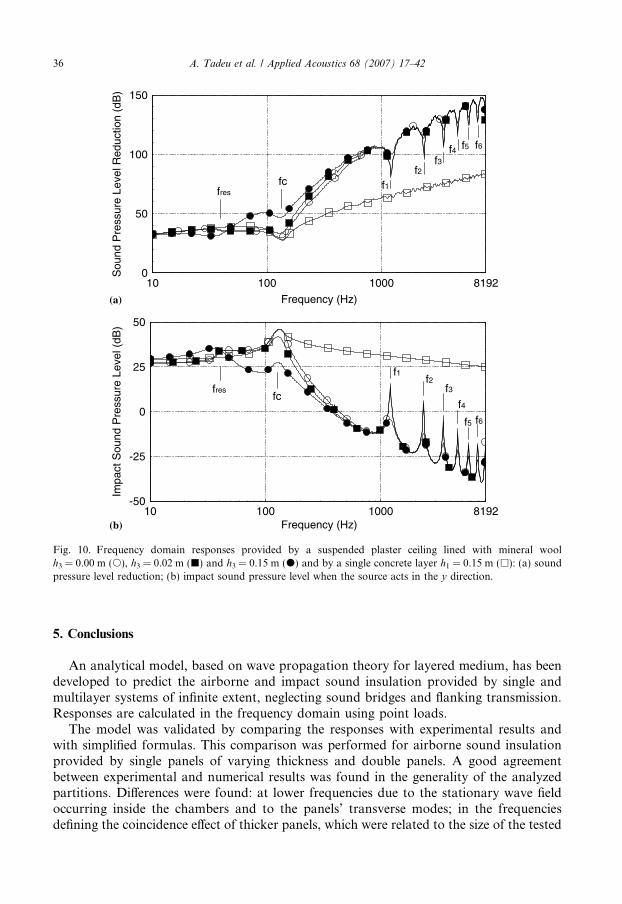
Fig. 10 displays both the sound pressure level reduction (Fig. 10a) and the impact soundpressure level (Fig. 10b) when there is no mineral wool layer present (h3 = 0.00 m – emptyair gap), and for h3 = 0.02 m and h3 = 0.15 m (fully-filled) thick mineral wool layers.Responses obtained for a 0.15 m thick single concrete structural layer are used as a refer-ence. As before the source acts in the acoustic medium at (0.0 m; �2.0 m) and in the elasticmedium in the y direction at (0.0 m; 0.0 m).
All results show a decrease in insulation in the vicinity of the critical frequency asso-ciated with the propagation of guided waves along the concrete structural layer (labeledfc in the plots). The frequency associated with the mass–air–mass resonance (labeled fres
in the plots) occurs at low frequencies and produces a fall in insulation. The resonance ofthe mass–air–mass system predicted using expression (12) leads to fres = 38.1 Hz. Thisresult is similar to that provided by the analytical model. The propagation of guidedwaves along the plaster layer does not seem to be important. The resonances excitedinside the air gap create a sharp dip in insulation at specific frequencies, labeled in theplot as f1, f2, . . . , f6. These frequencies can be predicted by fm = cm/(2h2), m = 1,2, . . . ,where h2 refers to the thickness of the air gap. According to the analytical model, theylie at higher frequencies than those predicted by this expression. It should be noted thatthe simplified expression assumes that the source only emits plane waves that travel per-pendicularly to the panel. When the mineral wool quilt is placed inside the air layer, theresonance effect inside the air gap and the coincidence effect are both attenuated, andinsulation improves in the vicinity of these frequencies. Notice that the insulation pro-vided by the concrete structural layer with a suspended ceiling layer is much better thanthat provided by a single 0.15 m concrete structural layer for the range of frequenciesanalyzed.
0
50
100
150
10 100 1000 8192
f6f5f4f3
f2f1fc
fres
Frequency (Hz)
Frequency (Hz)
Sou
nd P
ress
ure
Leve
l Red
uctio
n (d
B)
(a)
-50
-25
0
25
50
10 100 1000 8192
f6f5
f4
f3f2
f1
fcfres
Impa
ct S
ound
Pre
ssur
e Le
vel (
dB)
(b)
Fig. 10. Frequency domain responses provided by a suspended plaster ceiling lined with mineral woolh3 = 0.00 m (s), h3 = 0.02 m (j) and h3 = 0.15 m (d) and by a single concrete layer h1 = 0.15 m (h): (a) soundpressure level reduction; (b) impact sound pressure level when the source acts in the y direction.
36 A. Tadeu et al. / Applied Acoustics 68 (2007) 17–42
5. Conclusions
An analytical model, based on wave propagation theory for layered medium, has beendeveloped to predict the airborne and impact sound insulation provided by single andmultilayer systems of infinite extent, neglecting sound bridges and flanking transmission.Responses are calculated in the frequency domain using point loads.
The model was validated by comparing the responses with experimental results andwith simplified formulas. This comparison was performed for airborne sound insulationprovided by single panels of varying thickness and double panels. A good agreementbetween experimental and numerical results was found in the generality of the analyzedpartitions. Differences were found: at lower frequencies due to the stationary wave fieldoccurring inside the chambers and to the panels’ transverse modes; in the frequenciesdefining the coincidence effect of thicker panels, which were related to the size of the tested
A. Tadeu et al. / Applied Acoustics 68 (2007) 17–42 37
panels. It was found that the results provided by the analytical model show a better agree-ment with the experimental results than those provided by the mass law. Impact soundinsulation was also calculated for a single panel and a floating layer system and validationwas performed with experimental results. Again the analytical responses are quite similarto the experimental ones. The major differences are located at the lower frequencies in thevicinity of the coincidence effect.
The applicability of the analytical solutions to the prediction of the acoustic behavior ofa single structural layer and a suspended ceiling configuration was then discussed. It wasshown that the proposed model is able to capture all the physical acoustic phenomenainvolved in the prediction of the acoustic behavior provided by single and multilayer sys-tems of infinite extent, such as: the mass–air–mass resonance phenomena, the coincidenceeffect associated with the propagation of guided waves of the individual panels, the reso-nances excited inside the air gap and the effect of having the air layer filled with mineralwool.
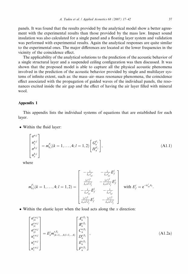
Appendix 1
This appendix lists the individual systems of equations that are established for eachlayer.
� Within the fluid layer:
ra;j
ua;jy
rb;j
ub;jy
266664
377775 ¼ mF j
k;lðk ¼ 1; . . . ; 4; l ¼ 1; 2Þ GF jn
HF jn
" #; ðA1:1Þ
where
mF j
k;lðk ¼ 1; . . . ; 4; l ¼ 1; 2Þ ¼
� iLxm
jnf
� iLxm
jnf
Ejf
ðcjÞ2
Lxx2kjf
� ðcjÞ2
Lxx2kjf
Ejf
� iLxm
jnf
Ejf � i
Lxmjnf
ðcjÞ2
Lxx2kjf
Ejf � ðcjÞ2
Lxx2kjf
2666666664
3777777775
with Ejf ¼ e�imj
nf hj :
� Within the elastic layer when the load acts along the x direction:
rx;a;jyx
rx;a;jyz
rx;a;jyy
ux;a;jx
ux;a;jy
ux;a;jz
2666666664
3777777775¼ Ej
amx;Sj
ðk¼1;...;6;l¼1;...;6Þ
Ax;Sjn
Bx;Sjn
Cx;Sjn
Dx;Sjn
Ex;Sjn
F x;Sjn
2666666664
3777777775; ðA1:2aÞ
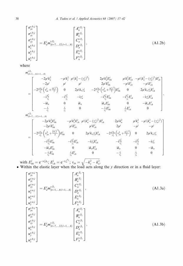
38 A. Tadeu et al. / Applied Acoustics 68 (2007) 17–42
rx;b;jyx
rx;b;jyz
rx;b;jyy
ux;b;jx
ux;b;jy
ux;b;jz
26666666664
37777777775¼ Ej
amx;Sj
ðk¼7;...;12;l¼1;...;6Þ
Ax;Sjn
Bx;Sjn
Cx;Sjn
Dx;Sjn
Ex;Sjn
F x;Sjn
2666666664
3777777775; ðA1:2bÞ
where
mx;Sj
ðk¼1;...;6;l¼1;...;6Þ
¼
�2ljk2n �ljk2
z ljðk2n�ðcj
nÞ2Þ 2ljk2
nEjbh ljk2
z Ejch �ljðk2
n�ðcjnÞ
2ÞEjch
�2lj lj lj 2ljEjbh �ljEj
ch �ljEjch
�2ljkn
mjn
m2znþ
ðkjsÞ22
� �0 2ljkncj
n �2ljkn
mjn
m2znþ
ðkjsÞ22
� �Ej
bh 0 2ljkncjnEj
ch
�i k2n
mjn
�i k2z
cjn
�icjn �i k2
n
mjnEj
bh �i k2z
cjnEj
ch �icjnEj
ch
�ikn 0 ikn iknEjbh 0 �iknEj
ch
� imj
n
icj
n0 � i
mjnEj
bhicj
nEj
ch 0
2666666666664
3777777777775;
mx;Sj
ðk¼7;...;12;l¼1;...;6Þ
¼
�2ljk2nEj
bh �ljk2z Ej
ch ljðk2n�ðcj
nÞ2ÞEj
ch 2ljk2n ljk2
z �ljðk2n�ðcj
nÞ2Þ
�2ljEjbh ljEj
ch ljEjch 2lj �lj �lj
�2ljkn
mjn
m2znþ
kjsð Þ22
� �Ej
bh 0 2ljkncjnEj
ch �2ljkn
mjn
m2znþ
ðkjsÞ22
� �0 2ljkncj
n
�i k2n
mjnEj
bh �i k2z
cjnEj
ch �icjnEj
ch �i k2n
mjn
�i k2z
cjn
�icjn
�iknEjbh 0 iknEj
ch ikn 0 �ikn
� imj
nEj
bhicj
nEj
ch 0 � imj
n
icj
n0
26666666666664
37777777777775
with Ejbh ¼ e�imj
nhj ; Ejch ¼ e�icj
nhj
; mzn ¼ffiffiffiffiffiffiffiffiffiffiffiffiffiffiffiffiffiffi�k2
z � k2n
q.
� Within the elastic layer when the load acts along the y direction or in a fluid layer:
ry;a;jyx
ry;a;jyz
ry;a;jyy
uy;a;jx
uy;a;jy
uy;a;jz
2666666664
3777777775¼ Ej
amy;Sj
ðk¼1;...;6;l¼1;...;6Þ
Ay;Sjn
By;Sjn
Cy;Sjn
Dy;Sjn
Ey;Sjn
F y;Sjn
2666666664
3777777775; ðA1:3aÞ
ry;b;jyx
ry;b;jyz
ry;b;jyy
uy;b;jx
uy;b;jy
uy;b;jz
26666666664
37777777775¼ Ej
amy;Sj
ðk¼7;...;12;l¼1;...;6Þ
Ay;Sjn
By;Sjn
Cy;Sjn
Dy;Sjn
Ey;Sjn
F y;Sjn
2666666664
3777777775; ðA1:3bÞ
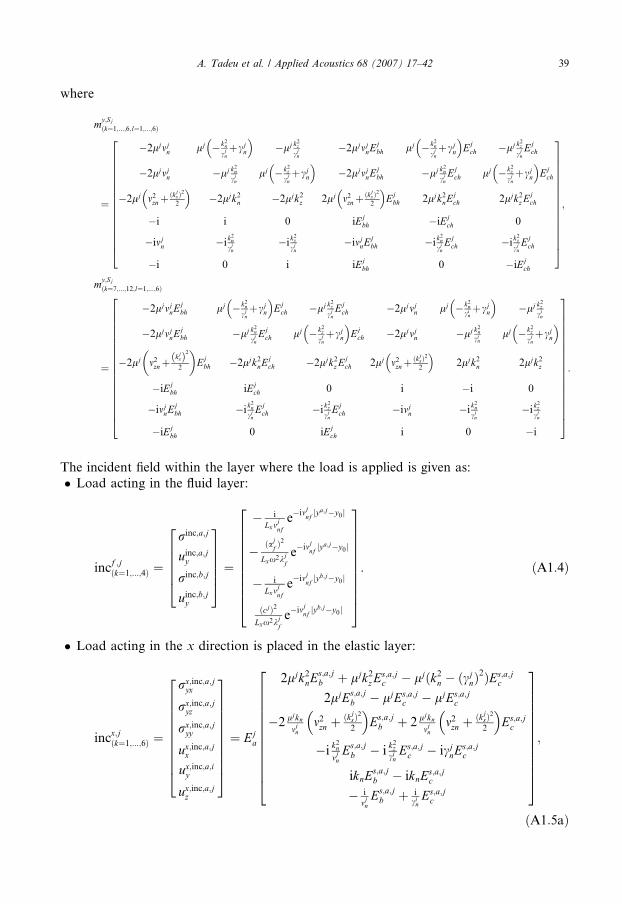
A. Tadeu et al. / Applied Acoustics 68 (2007) 17–42 39
where
my;Sj
ðk¼1;...;6;l¼1;...;6Þ
¼
�2ljmjn lj �k2
n
cjnþcj
n
� ��lj k2
z
cjn
�2ljmjnEj
bh lj �k2n
cjnþcj
n
� �Ej
ch �lj k2z
cjnEj
ch
�2ljmjn �lj k2
n
cjn
lj �k2z
cjnþcj
n
� ��2ljmj
nEjbh �lj k2
n
cjnEj
ch lj �k2z
cjnþcj
n
� �Ej
ch
�2lj m2znþ
ðkjsÞ22
� ��2ljk2
n �2ljk2z 2lj m2
znþðkj
sÞ22
� �Ej
bh 2ljk2nEj
ch 2ljk2z Ej
ch
�i i 0 iEjbh �iEj
ch 0
�imjn �ik2
n
cjn
�ik2z
cjn
�imjnEj
bh �i k2n
cjnEj
ch �ik2z
cjnEj
ch
�i 0 i iEjbh 0 �iEj
ch
2666666666666664
3777777777777775
;
my;Sj
ðk¼7;...;12;l¼1;...;6Þ
¼
�2ljmjnEj
bh lj �k2n
cjnþcj
n
� �Ej
ch �lj k2z
cjnEj
ch �2ljmjn lj �k2
nci
nþcj
n
� ��lj k2
z
cjn
�2ljmjnEj
bh �lj k2n
cjnEj
ch lj �k2z
cjnþcj
n
� �Ej
ch �2ljmjn �lj k2
nci
nlj �k2
z
cjnþcj
n
� �
�2lj m2znþ
kjsð Þ22
� �Ej
bh �2ljk2nEj
ch �2ljk2z Ej
ch 2lj m2znþ
ðkjsÞ22
� �2ljk2
n 2ljk2z
�iEjbh iEj
ch 0 i �i 0
�imjnEj
bh �i k2n
cjnEj
ch �ik2z
cjnEj
ch �imjn �i k2
n
cjn
�i k2z
cjn
�iEjbh 0 iEj
ch i 0 �i
266666666666666664
377777777777777775
:
The incident field within the layer where the load is applied is given as:� Load acting in the fluid layer:
incf ;jðk¼1;...;4Þ ¼
rinc;a;j
uinc;a;jy
rinc;b;j
uinc;b;jy
266664
377775 ¼
� iLxm
jnf
e�imjnf jy
a;j�y0j
� ðajf Þ
2
Lxx2kjf
e�imjnf jy
a;j�y0j
� iLxm
jnf
e�imjnf jy
b;j�y0j
ðcjÞ2
Lxx2kjf
e�imjnf jy
b;j�y0j
26666666664
37777777775: ðA1:4Þ
� Load acting in the x direction is placed in the elastic layer:
incx;jðk¼1;...;6Þ ¼
rx;inc;a;jyx
rx;inc;a;jyz
rx;inc;a;jyy
ux;inc;a;jx
ux;inc;a;iy
ux;inc;a;jz
26666666664
37777777775¼ Ej
a
2ljk2nEs;a;j
b þ ljk2z Es;a;j
c � ljðk2n � ðcj
nÞ2ÞEs;a;j
c
2ljEs;a;jb � ljEs;a;j
c � ljEs;a;jc
�2 ljkn
mjn
m2zn þ
ðkjsÞ22
� �Es;a;j
b þ 2 ljkn
mjn
m2zn þ
ðkjsÞ22
� �Es;a;j
c
�i k2n
mjnEs;a;j
b � i k2z
cinEs;a;j
c � icjnEs;a;j
c
iknEs;a;jb � iknEs;a;j
c
� imj
nEs;a;j
b þ ici
nEs;a;j
c
2666666666664
3777777777775;
ðA1:5aÞ
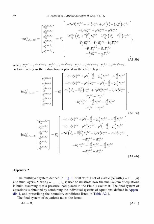
40 A. Tadeu et al. / Applied Acoustics 68 (2007) 17–42
incx;jðk¼7;...;12Þ ¼
rx;inc;b;jyx
rx;inc;b;jyz
rx;inc;b;jyy
ux;inc;b;jx
ux;inc;b;jy
ux;inc;b;jz
2666666664
3777777775¼ Ej
a
�2ljk2nEs;b;j
b � ljk2z Es;b;j
c þ lj k2n � ðcj
nÞ2
� �Es;b;j
c
�2ljEs;b;jb þ ljEs;b;j
c þ ljEs;b;jc
�2 ljkn
mjn
m2zn þ
ðkjsÞ22
� �Es;b;j
b þ 2 ljkn
mjn
m2zn þ
ðkjsÞ22
� �Es;b;j
c
�i k2n
mjnEs;b;j
b � i k2z
cjnEs;b;j
c � icjnEs;b;j
c
�iknEs;b;jb þ iknEs;b;j
c
� imj
nEs;b;j
b þ icj
nEs;b;j
c
26666666666664
37777777777775;
ðA1:5bÞwhere Es;a;j
b ¼ e�imjnjya;j�y0j; Es;b;j
b ¼ e�imjnjyb;j�y0j; Es;a;j
c ¼ e�icjnjya;j�y0j; Es;b;j
c ¼ e�icjnjyb;j�y0j.
� Load acting in the y direction is placed in the elastic layer:
incy;jðk¼1;...;6Þ ¼
ry;inc;a;jyx
ry;inc;a;jyz
ry;inc;a;jyy
uy;inc;a;jx
uy;inc;a;jy
uy;inc;a;jz
26666666664
37777777775¼ Ej
a
�2ljmjnEs;a;j
b þ lj � k2n
cjnþ cj
n
� �Es;a;j
c � lj k2z
cjnEs;a;j
c
�2ljmjnEs;a;j
b � lj k2n
cjnEs;a;j
c þ lj � k2n
cjnþ cj
n
� �Es;a;j
c
2lj m2zn þ
ðkjsÞ22
� �Es;a;j
b þ 2ljk2nEs;a;j
c þ 2ljk2z Es;a;j
c
iEs;a;jb � iEs;a;j
c
�imjnEs;a;j
b � i k2n
cjnEs;a;j
c � i k2z
cinEs;a;j
c
iEs;a;jb � iEs;a;j
c
266666666666664
377777777777775;
ðA1:6aÞ
incy;jðk¼7;...;12Þ
ry;inc;b;jyx
ry;inc;b;jyz
ry;inc;b;jyy
uy;inc;b;jx
uy;inc;b;jy
uy;inc;b;jz
26666666664
37777777775¼ Ej
a
�2ljmjnEs;b;j
b þ lj � k2n
cjnþ cj
n
� �Es;b;j
c � lj k2z
cjnEs;b;j
c
�2ljmjnEs;b;j
b � lj k2n
cjnEs;b;j
c þ lj � k2n
cjnþ cj
n
� �Es;b;j
c
�2lj m2zn þ
ðkjsÞ22
� �Es;b;j
b � 2ljk2nEs;b;j
c � 2ljk2z Es;b;j
c
�iEs;b;jb þ iEs;b;j
c
�imjnEs;b;j
b � i k2n
cjnEs;b;j
c � i k2z
cjnEs;b;j
c
�iEs;b;jb þ iEs;b;j
c
266666666666664
377777777777775:
ðA1:6bÞ
Appendix 2
The multilayer system defined in Fig. 1, built with a set of elastic (Sj with j = 1, . . . ,n)and fluid layers (Fj with j = 1, . . . ,n), is used to illustrate how the final system of equationsis built, assuming that a pressure load placed in the Fluid 1 excites it. The final system ofequations is obtained by combining the individual systems of equations, defined in Appen-dix 1, and prescribing the boundary conditions listed in Table A2.1.
The final system of equations takes the form:
AX ¼ B; ðA2:1Þ
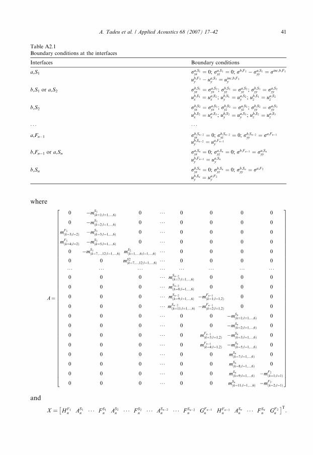
Table A2.1Boundary conditions at the interfaces
Interfaces Boundary conditions
a,S1 ra;S1yx ¼ 0; ra;S1
yz ¼ 0; rb;F 1 � ra;S1yy ¼ rinc;b;F 1
ub;F 1y � ua;S1
y ¼ uinc;b;F 1y
b,S1 or a,S2 rb;S1yx ¼ ra;S2
yx ; rb;S1yz ¼ ra;S2
yz ; rb;S1yy ¼ ra;S2
yy
ub;S1x ¼ ua;S2
x ; ub;S1y ¼ ua;S2
y ; ub;S1z ¼ ua;S2
z
b,S2 rb;S2yx ¼ ra;S3
yx ; rb;S2yz ¼ ra;S3
yz ; rb;S2yy ¼ ra;S3
yy
ub;S2x ¼ ua;S3
x ; ub;S2y ¼ ua;S3
y ; ub;S2z ¼ ua;S3
z
� � � � � �
a,Fn�1 rb;Sn�2yx ¼ 0; rb;Sn�2
yz ¼ 0; rb;Sn�2yy ¼ ra;F n�1
ub;Sn�2y ¼ ua;F n�1
y
b,Fn�1 or a,Sn ra;Snyx ¼ 0; ra;Sn
yz ¼ 0; rb;F n�1 ¼ ra;Snyy
ub;F n�1y ¼ ua;Sn
y
b,Sn rb;Snyx ¼ 0; rb;Sn
yz ¼ 0; rb;Snyy ¼ ra;F 2
ub;Sny ¼ ua;F 2
y
A. Tadeu et al. / Applied Acoustics 68 (2007) 17–42 41
where
A¼
0 �mS1
ðk¼1;l¼1;...;6Þ 0 � � � 0 0 0 0
0 �mS1
ðk¼2;l¼1;...;6Þ 0 � � � 0 0 0 0
mF 1
ðk¼3;l¼2Þ �mS1
ðk¼3;l¼1;...;6Þ 0 � � � 0 0 0 0
mF 1
ðk¼4;l¼2Þ �mS1
ðk¼5;l¼1;...;6Þ 0 � � � 0 0 0 0
0 �mS1
ðk¼7;...;12;l¼1;...;6Þ mS2
ðk¼1;...;6;l¼1;...;6Þ � � � 0 0 0 0
0 0 mS2ðk¼7;...;12;l¼1;...;6Þ � � � 0 0 0 0
� �� �� � � � � � � � � �� � � � � �� �� �0 0 0 � � � mSn�2
ðk¼7;l¼1;...;6Þ 0 0 0
0 0 0 � � � mSn�2
ðk¼8;l¼1;...;6Þ 0 0 0
0 0 0 � � � mSn�2
ðk¼9;l¼1;...;6Þ �mF n�1
ðk¼1;l¼1;2Þ 0 0
0 0 0 � � � mSn�2
ðk¼11;l¼1;...;6Þ �mF n�1
ðk¼2;l¼1;2Þ 0 0
0 0 0 � � � 0 0 �mSnðk¼1;l¼1;...;6Þ 0
0 0 0 � � � 0 0 �mSnðk¼2;l¼1;...;6Þ 0
0 0 0 � � � 0 mF n�1
ðk¼3;l¼1;2Þ �mSnðk¼3;l¼1;...;6Þ 0
0 0 0 � � � 0 mF n�1
ðk¼4;l¼1;2Þ �mSnðk¼5;l¼1;...;6Þ 0
0 0 0 � � � 0 0 mSnðk¼7;l¼1;...;6Þ 0
0 0 0 � � � 0 0 mSnðk¼8;l¼1;...;6Þ 0
0 0 0 � � � 0 0 mSnðk¼9;l¼1;...;6Þ �mF 2
ðk¼1;l¼1Þ
0 0 0 � � � 0 0 mSnðk¼11;l¼1;...;6Þ �mF 2
ðk¼2;l¼1Þ
2666666666666666666666666666666666666666666666666664
3777777777777777777777777777777777777777777777777775
and
X ¼ H F 1n AS1
n � � � F S1n AS2
n � � � F S2n � � � ASn�2
n � � � F Sn�2n GF n�1
n H F n�1n ASn
n � � � F Snn GF 2
n
T:
42 A. Tadeu et al. / Applied Acoustics 68 (2007) 17–42
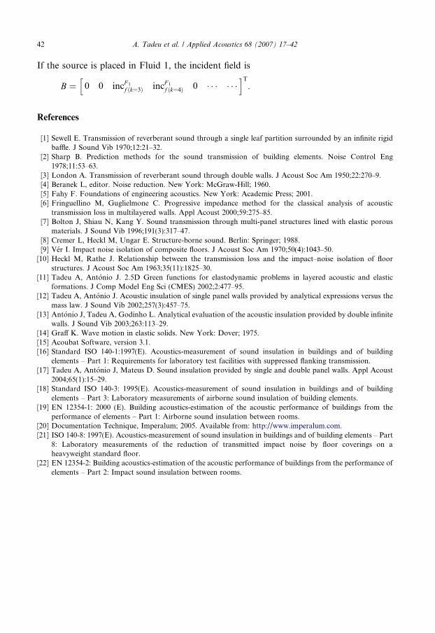
If the source is placed in Fluid 1, the incident field is
B ¼ 0 0 incF 1
f ðk¼3Þ incF 1
f ðk¼4Þ 0 � � � � � �h iT
:
References
[1] Sewell E. Transmission of reverberant sound through a single leaf partition surrounded by an infinite rigidbaffle. J Sound Vib 1970;12:21–32.
[2] Sharp B. Prediction methods for the sound transmission of building elements. Noise Control Eng1978;11:53–63.
[3] London A. Transmission of reverberant sound through double walls. J Acoust Soc Am 1950;22:270–9.[4] Beranek L, editor. Noise reduction. New York: McGraw-Hill; 1960.[5] Fahy F. Foundations of engineering acoustics. New York: Academic Press; 2001.[6] Fringuellino M, Guglielmone C. Progressive impedance method for the classical analysis of acoustic
transmission loss in multilayered walls. Appl Acoust 2000;59:275–85.[7] Bolton J, Shiau N, Kang Y. Sound transmission through multi-panel structures lined with elastic porous
materials. J Sound Vib 1996;191(3):317–47.[8] Cremer L, Heckl M, Ungar E. Structure-borne sound. Berlin: Springer; 1988.[9] Ver I. Impact noise isolation of composite floors. J Acoust Soc Am 1970;50(4):1043–50.
[10] Heckl M, Rathe J. Relationship between the transmission loss and the impact–noise isolation of floorstructures. J Acoust Soc Am 1963;35(11):1825–30.
[11] Tadeu A, Antonio J. 2.5D Green functions for elastodynamic problems in layered acoustic and elasticformations. J Comp Model Eng Sci (CMES) 2002;2:477–95.
[12] Tadeu A, Antonio J. Acoustic insulation of single panel walls provided by analytical expressions versus themass law. J Sound Vib 2002;257(3):457–75.
[13] Antonio J, Tadeu A, Godinho L. Analytical evaluation of the acoustic insulation provided by double infinitewalls. J Sound Vib 2003;263:113–29.
[14] Graff K. Wave motion in elastic solids. New York: Dover; 1975.[15] Acoubat Software, version 3.1.[16] Standard ISO 140-1:1997(E). Acoustics-measurement of sound insulation in buildings and of building
elements – Part 1: Requirements for laboratory test facilities with suppressed flanking transmission.[17] Tadeu A, Antonio J, Mateus D. Sound insulation provided by single and double panel walls. Appl Acoust
2004;65(1):15–29.[18] Standard ISO 140-3: 1995(E). Acoustics-measurement of sound insulation in buildings and of building
elements – Part 3: Laboratory measurements of airborne sound insulation of building elements.[19] EN 12354-1: 2000 (E). Building acoustics-estimation of the acoustic performance of buildings from the
performance of elements – Part 1: Airborne sound insulation between rooms.[20] Documentation Technique, Imperalum; 2005. Available from: http://www.imperalum.com.[21] ISO 140-8: 1997(E). Acoustics-measurement of sound insulation in buildings and of building elements – Part
8: Laboratory measurements of the reduction of transmitted impact noise by floor coverings on aheavyweight standard floor.
[22] EN 12354-2: Building acoustics-estimation of the acoustic performance of buildings from the performance ofelements – Part 2: Impact sound insulation between rooms.