Predicting Vehicle Crashworthiness:Validation of Computer Models forFunctional and Hierarchical Data

M. J. Bayarri, James O. Berger, Marc C. Kennedy, Athanasios Kottas,

Rui Paulo, Jerry Sacks, John A. Cafeo, Chin-Hsu Lin, and Jian Tu ∗

Abstract

The CRASH computer model simulates the effect of a vehicle colliding

against different barrier types. If it accurately represents real vehicle crash-

worthiness, the computer model can be of great value in various aspects of

vehicle design, such as the setting of timing of air bag releases. The goal of

this study is to address the problem of validating the computer model for such

design goals, based on utilizing computer model runs and experimental data

from real crashes. This task is complicated by the fact that (i) the output of

this model consists of smooth functional data, and (ii) certain types of collision

have very limited data. We address problem (i) by extending existing Gaus-

sian process-based methodology developed for models that produce real-valued

output, and resort to Bayesian hierarchical modeling to attack problem (ii).

∗M. J. Bayarri is Professor, Department of Statistics and Operations Research, University ofValencia, Valencia, Spain (E-mail: Susie.Bayarri@uv.es). James O. Berger is the Arts and SciencesProfessor of Statistics, Department of Statistical Science, Duke University, Durham, NC 27708 (E-mail: berger@stat.duke.edu). Marc C. Kennedy is Senior Risk Analyst, Central Science Laboratory,Sand Hutton, York YO41 1LZ, U.K. (E-mail: m.kennedy@csl.gov.uk). Athanasios Kottas is Asso-ciate Professor, Department of Applied Mathematics and Statistics, University of California, SantaCruz, CA 95064 (E-mail: thanos@ams.ucsc.edu). Rui Paulo is Assistant Professor, Department ofMathematics, ISEG, Technical University of Lisbon, Portugal (E-mail: rui@iseg.utl.pt). Jerry Sacksis Director Emeritus and Senior Fellow, National Institute of Statistical Sciences, Research TrianglePark, NC 27709 (E-mail: sacks@niss.org). John A. Cafeo, Chin-Hsu Lin, and Jian Tu are withResearch and Development, General Motors, Warren, MI 48090. This research was supported inpart by grants from General Motors and the National Science Foundation (Grant DMS-0073952)to the National Institute of Statistical Sciences. The authors thank the editor, David Banks, anassociate editor, and two referees for their valuable comments and suggestions.

1

Additionally, we show how to formally test if the computer model reproduces

reality. (Supplemental materials for the article are available on-line.)

KEY WORDS: Air bag timing; Bayesian analysis; Bias; Hierarchical modeling;

Hypothesis testing; Validation; Vehicle design.

1 INTRODUCTION

1.1 The Computer Model for Vehicle Crashworthiness

The CRASH computer model simulates the effect of a collision of a vehicle with dif-

ferent types of barriers. Proving ground tests with prototype vehicles must ultimately

be made to meet mandated standards for crashworthiness, but the computer model

plays an integral part in the design of the vehicle to assure crashworthiness before

manufacturing the prototypes. How well the model performs is therefore crucial to

the vehicle design process.

CRASH is implemented using a non-linear dynamic analysis (commercial) code,

LS-DYNA, using a finite element representation of the vehicle. The main focus is on

the velocity changes after impact at key positions on the vehicle.

Geometric representation of the vehicle and the material properties play critical

roles in the behavior of the vehicle after impact and the necessary detailing of these

inputs leads to very time consuming computer runs (from 1 to 5 days on a standard

workstation). Obtaining field data involves crashing of full vehicles, so that field data

is obviously also limited. Studying CRASH is thus inherently data-limited — both in

terms of computer runs and field data — presenting a basic challenge to assessing the

validity of the computer model in accurately representing real vehicle crashworthiness.

There are many variables and sources of uncertainty in the vehicle manufacturing

process and proving ground test procedures that, in turn, induce uncertainties in

the test results. The acceleration and velocity histories (i.e., the acceleration and

2

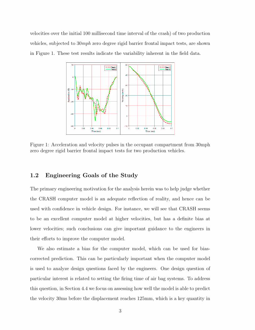
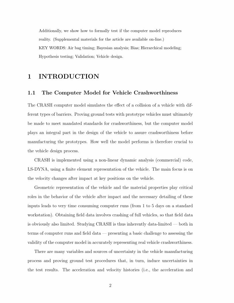
velocities over the initial 100 millisecond time interval of the crash) of two production

vehicles, subjected to 30mph zero degree rigid barrier frontal impact tests, are shown

in Figure 1. These test results indicate the variability inherent in the field data.

Figure 1: Acceleration and velocity pulses in the occupant compartment from 30mphzero degree rigid barrier frontal impact tests for two production vehicles.

1.2 Engineering Goals of the Study

The primary engineering motivation for the analysis herein was to help judge whether

the CRASH computer model is an adequate reflection of reality, and hence can be

used with confidence in vehicle design. For instance, we will see that CRASH seems

to be an excellent computer model at higher velocities, but has a definite bias at

lower velocities; such conclusions can give important guidance to the engineers in

their efforts to improve the computer model.

We also estimate a bias for the computer model, which can be used for bias-

corrected prediction. This can be particularly important when the computer model

is used to analyze design questions faced by the engineers. One design question of

particular interest is related to setting the firing time of air bag systems. To address

this question, in Section 4.4 we focus on assessing how well the model is able to predict

the velocity 30ms before the displacement reaches 125mm, which is a key quantity in

3

determining when an airbag should be fired (see also Section 2.4).

Our statistical analysis also involves development of an emulator of the computer

model, which is simply a fast numerical approximation to the computer model. It

will be seen that this emulator is itself accurate enough for use in the analysis of this

design question, thus allowing much more intensive exploration of design space than

would be possible if the computer model itself had to be run at all potential design

points.

1.3 Statistical Background

General discussions of the entire Validation and Verification process for computer

models can be found in Roache (1998), Oberkampf and Trucano (2000), Pilch et al.

(2001), Trucano et al. (2002), and Santner et al. (2003). We focus here on the

last stage of the process: that of assessing the accuracy of the computer model in

predicting reality, and in using both the computer model and field data to make

predictions, especially in new situations.

Because a computer model can virtually never be said to be a completely accurate

representation of the real process being modeled, the relevant question is “Does the

model provide predictions that are accurate enough for its intended use?” Thus

predictions need to come with what were called tolerance bounds in Bayarri et al.

(2007b), indicating the magnitude of the prediction error.

This focus on giving tolerance bounds, rather than stating a yes/no answer as

to model validity, arises for three reasons. First, models rarely give highly accurate

predictions over the entire range of inputs of possible interest, and it is often difficult

to characterize regions of accuracy and inaccuracy; for instance, we will see that, for

certain inputs, the computer model of vehicle crashworthiness yields quite accurate

predictions, while for others it does not. Second, the degree of accuracy that is needed

can vary from one application of the computer model to another, as will be seen in

4

study of the different uses of CRASH. Finally, tolerance bounds account for model

bias, the principal symptom of model inadequacy; accuracy of the model cannot

simply be represented by a variance or standard error.

The key components of the approach outlined here are the use of Gaussian process

response-surface approximations to a computer model, following on work in Sacks

et al. (1989), Currin et al. (1991), Welch et al. (1992), and Morris et al. (1993),

and introduction of Bayesian representations of model bias and uncertainty, following

on work in Kennedy and O’Hagan (2001) and Kennedy et al. (2002); Higdon et al.

(2004), Lee et al. (2006), Campbell (2006), Gramacy and Lee (2006) and Gramacy

and Lee (2008) are more recent references. A related approach to Bayesian analysis

of computer models is that of Craig et al. (1997), Craig et al. (2001), Goldstein and

Rougier (2003) and Goldstein and Rougier (2004), and Goldstein and Wooff (2007)

which focus on utilization of linear Bayes methodology to address the problem.

1.4 Required Methodological Extensions

Bayarri et al. (2007b) described a general framework for validation of complex com-

puter models and applied the framework to two examples. The extensions of this

methodology that were needed to deal with the CRASH model were the following:

Problem 1 – Smooth Functional Output: In Bayarri et al. (2007b), the exam-

ples considered involved real-valued model outputs. The output of CRASH, however,

is a time-dependent function. Thus, in validating the computer model with field data,

one must compare functions, a more difficult enterprise.

Problem 2 – Hierarchical Modeling: A common problem in computer modeling

is that codes (and field experiments) can be run under differing conditions, where

the differences are not completely quantifiable and where data may be scant – or

even lacking – for some of the conditions. In CRASH, this arises when treating

5

collisions of different barriers; there are few data for center pole collision or for right-

angle collision, but there are reasonable amounts of data for straight-frontal and

left-angle collision (see Table 1). Therefore, using hierarchical modeling, data from

the various experiments can be combined to obtain improved predictions. In addition,

the methods can be used for prediction under untried conditions, as long as the new

conditions are deemed to be compatible with the hierarchical modeling assumptions,

although the uncertainties associated with these predictions may be quite large.

Problem 3 – Testing Model Correctness: The validation question initially

asked by many computer modelers is “Can you establish that the computer model

is correct?” In Section 6 it is shown how one can formally conduct a test to answer

this question. The result of the test will virtually always be that there is conclusive

evidence that the computer model is not correct, but formally providing an answer

to this question can be of pedagogical value.

1.5 Overview

Section 2 outlines the key elements of the problem, and discusses the basic strategy

that is utilized to deal with functional data. Approximation of the computer model is

considered in Section 3, while the Bayesian validation analysis is given in Section 4.

Section 5 introduces the hierarchical methodology for dealing with related scenarios

(differing barrier collisions in CRASH), while Section 6 considers the formal testing

of model validity. Finally, Section 7 concludes with a summary of our findings for the

CRASH model, and a technical summary of the methodology.

Most of the details of the computations are relegated to the Appendix and to a

companion technical report, Bayarri et al. (2005), which is available on-line under

“Supplementary Material” at http://pubs.amstat.org/loi/jasa.

6

2 KEY ELEMENTS OF THE PROBLEM

2.1 Inputs

The inputs to the computer model will be denoted by a vector x. In the case of

CRASH, the two key inputs are x1 = velocity at impact and barrier type. Of course,

the computer model has numerous other inputs (indeed thousands, if one counts

the finite-element basis of the computer model) but, for this case-study, the desired

engineering focus was in studying the computer model in terms of these two inputs.

The methodology from Bayarri et al. (2007b) that we are adopting does not ac-

commodate qualitative inputs such as barrier type. Hence, to deal with the full range

of barrier types, we will resort to hierarchical analysis. However, three of the barrier

types (left angle, straight frontal, and right angle) can be converted into the quan-

titative input x2 = angle of impact. For most of the paper, we will analyze only the

data for straight frontal collision (the most extensive data set), and will then be using

x to just represent impact velocity, but in Section 5 we also consider angle and x will

then represent the pair (impact velocity, angle).

In CRASH, the selected inputs for running the computer model and collecting

field data were chosen for reasons other than conducting a model validation (and

before the initiation of this work), and are given in Table 1; note that replicates exist

of the field data, which is highly useful for model validation.

Each computer run or field test resulted in acceleration data curves as in the left

panel of Figure 1, corresponding to various locations on the vehicle. (For the field

data, these acceleration curves were from sensors placed at various locations.) The

primary output of interest, and that which we shall focus on here, is the relative

velocity of the “Sensing and Diagnostic Module”, SDM, situated under the driver’s

seat, relative to a free-flight dummy. This relative velocity is obtained by integrating

the observed SDM acceleration curves and then subtracting the impact velocity x1

7

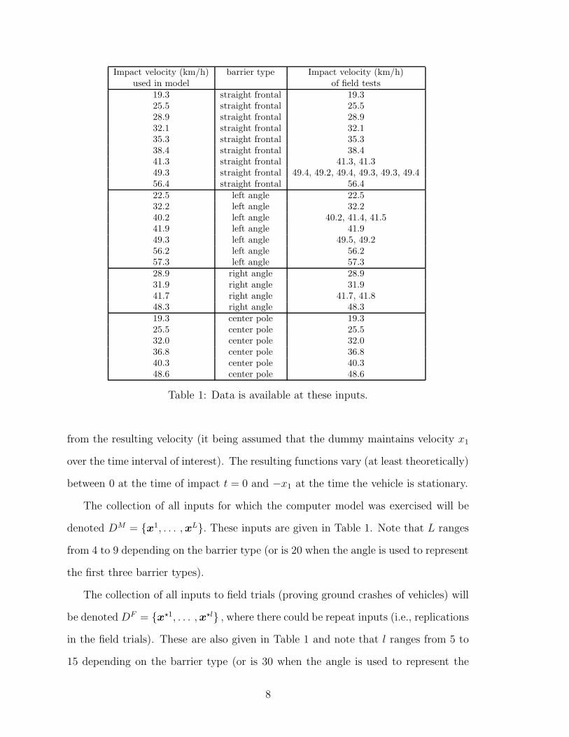
Impact velocity (km/h) barrier type Impact velocity (km/h)used in model of field tests

19.3 straight frontal 19.325.5 straight frontal 25.528.9 straight frontal 28.932.1 straight frontal 32.135.3 straight frontal 35.338.4 straight frontal 38.441.3 straight frontal 41.3, 41.349.3 straight frontal 49.4, 49.2, 49.4, 49.3, 49.3, 49.456.4 straight frontal 56.422.5 left angle 22.532.2 left angle 32.240.2 left angle 40.2, 41.4, 41.541.9 left angle 41.949.3 left angle 49.5, 49.256.2 left angle 56.257.3 left angle 57.328.9 right angle 28.931.9 right angle 31.941.7 right angle 41.7, 41.848.3 right angle 48.319.3 center pole 19.325.5 center pole 25.532.0 center pole 32.036.8 center pole 36.840.3 center pole 40.348.6 center pole 48.6

Table 1: Data is available at these inputs.

from the resulting velocity (it being assumed that the dummy maintains velocity x1

over the time interval of interest). The resulting functions vary (at least theoretically)

between 0 at the time of impact t = 0 and −x1 at the time the vehicle is stationary.

The collection of all inputs for which the computer model was exercised will be

denoted DM = x1, . . . , xL. These inputs are given in Table 1. Note that L ranges

from 4 to 9 depending on the barrier type (or is 20 when the angle is used to represent

the first three barrier types).

The collection of all inputs to field trials (proving ground crashes of vehicles) will

be denoted DF = x?1, . . . , x?l , where there could be repeat inputs (i.e., replications

in the field trials). These are also given in Table 1 and note that l ranges from 5 to

15 depending on the barrier type (or is 30 when the angle is used to represent the

8

first three barrier types).

2.2 Incorporating Functional Outputs

There are several possible approaches that can be taken to adapt the methods of

Bayarri et al. (2007b) to the setting of functional data of the type depicted in the

right panel of Figure 1.

One common approach is to represent the functions that arise through a basis

expansion (e.g., a polynomial expansion), taking only a finite number of terms of

the expansion to represent the function. The coefficients of the terms in this expan-

sion would then be viewed as a collection of real-valued output functions, with the

methodology from Bayarri et al. (2007b) being applied to each. Examples using a

wavelet basis for ‘rough’ output functions can be found in Bayarri et al. (2007a). See

also Higdon et al. (2008) for a related approach.

In our model, the functional data for velocity (which is the primary interest)

is rather smooth, and so we turn instead to the most direct possibility, which is to

combine t with x, thus enlarging the input space to z = (x, t). Since we only consider

discrete input values here, we further must assume that we have only observed the

function at a discrete set of points, DT = t1, . . . , tN. If N is chosen large enough and

the points at which we record the function are chosen well, then the function values

at these N points will adequately represent the entire function. Similar approaches

are taken in Conti and O’Hagan (2007), Rougier (2007), and McFarkand et al. (2008).

As will be seen in Section 3, it is computationally important to discretize all

functional outputs (model-run and field data) at the same set of time points DT . We

have chosen DT = 1, 3, 5, 7, 9, 11, 13, 15, 17, 20, 25, 30, 35, 40, 45, 50, 55, 60, 65, where

all measurements are in milliseconds (ms). More points were chosen in the region

t < 20ms, since information from this region will be seen to be more important in

estimating the primary quantity of interest, related to air bag firing. Times above

9

65 ms are unimportant for the same reason, and so there was no need to include

such points in the design. These 19 time points provide a good compromise between

adequate representation of the function (for the desired purposes) and numerical

efficiency.

2.3 Data

As discussed above, the data we analyze is the relative SDM velocity in the field

runs and computer model runs over the (augmented) input domains DF × DT and

DM ×DT . (The Cartesian product form arises because DT was chosen to be the same

for each function.) These data will be denoted by yM ≡ yM(x, t) : x ∈ DM , t ∈ DT

and yF ≡ yF (x, t) : x ∈ DF , t ∈ DT, vectors of lengths that we henceforth denote

by m and n, respectively, constructed from lexicographic ordering of the inputs.

2.4 Evaluation Criteria

Computer models are typically used for many purposes, so overall fidelity to reality

of the computer model predictions is an issue of considerable interest. Hence, we will

be interested in comparing the entire function predicted by the computer model with

the function observed from the field data, over a wide range of inputs.

We will also focus on a more specific feature that is of engineering interest, namely

the SDM velocity calculated 30ms before the time the SDM displacement (relative to

the free-flight dummy), DISP, reaches 125mm. Call this quantity CRITV. The air bag

takes around 30ms to fully deploy, which is why this particular evaluation criterion

is important. Our analysis takes account of the dependence between displacement

and velocity (displacement is the integral of velocity); it is a useful feature of the

Bayesian approach we adopt that dealing with composite criteria, such as this, is no

more difficult than dealing directly with the outputs.

10

3 APPROXIMATING THE COMPUTER MODEL

The CRASH model can take days to run, and a fast approximation – an emulator

– is needed for the statistical analysis (which we perform via Markov Chain Monte

Carlo simulation (MCMC), requiring thousands of computer model runs).

We denote the (now scalar) output of the CRASH model at input z = (x, t) by

yM(z). An expensive computer code, such as the one for the CRASH model, is only

run at some few inputs (here z ∈ DM×DT ) and should thus be viewed as an unknown

function at all other values of z. An emulator is an approximation yM(z), which

also has the desirable property of having a variance function V M(z) that measures

the accuracy of yM(z) as an estimate of yM(z). A response surface approach that

achieves both these goals is the Gaussian process response surface approximation

(GASP), described in Sacks et al. (1989) and Kennedy and O’Hagan (2001). We thus

assume that yM(z) has a prior distribution given by a Gaussian process with mean

µ(·), correlation function cM(·, ·), and unknown precision (1/variance)= λM , to be

denoted by GP( µ(·), 1λM cM(·, ·)).

Process mean: There is a clear trend in the velocity output, as can be seen in

the right panel of Figure 1 (although recall that we will be considering the relative

velocity, found by subtracting the initial impact velocity, x1). The relative velocity

thus starts at 0 and declines to a value near −x1, and hence it is reasonable to

introduce a term that reflects this trend, the simplest being of the form µMx1 t, with

µM being unknown.

Process correlation: We choose this to be of the form

cM(z, z?) = exp

(

−d∑

`=1

βM` |z` − z?

` |αM

`

)

. (3.1)

11

Here, d is the number of coordinates in z: either 2 or 3 for CRASH (with inputs

augmented by t), depending on whether angle is included as an input. The αM` take

values in (1, 2), and the βM` in (0,∞). The product form of the correlation function

(each factor is itself a correlation function in one dimension) facilitates the computa-

tions made later. Prior beliefs about the smoothness properties of the function will

affect the choice of αM = αM` : ` = 1, ..., d. For example, the choice αM

` = 2 for all

` reflects the belief that the function is infinitely differentiable, plausible for many en-

gineering models. We denote all the covariance parameters by θM = (λM , αM , βM),

where βM = βM` : ` = 1, ..., d.

Finite dimensional distribution: From the Gaussian process assumption, yM ,

conditional on the hyperparameters, is multivariate normal with covariance matrix

ΓM = CM(DM ×DT , DM ×DT )/λM , where CM(DM ×DT , DM ×DT ) is the matrix

with (i, j) entry cM(zi, zj), for each pair zi and zj in DM ×DT . Once yM is observed,

this yields a likelihood function for the parameters θM and µM based solely on the

observed yM .

Prediction (approximation) at a new input: Given yM and the unknown pa-

rameters µM and θM , yM(·) is again a Gaussian process with mean and covariance

functions given respectively by (see, for example, Stein (1999))

E[ yM(z) | yM , µM , θM ] = µMx1 t + rz

′(ΓM)−1(yM − µMΨ) (3.2)

Cov[ yM(z), yM(z?) | yM , µM , θM ] =1

λMcM(z, z?) − rz

′(ΓM)−1rz? , (3.3)

where rz′ = 1

λM (cM(z, z1), . . . , cM(z, zm)), ΓM is given above, and Ψ is the column

vector consisting of the values of x1 t corresponding to the inputs in DM × DT .

12

If z is a new input value, the response surface approximation to yM(z), given

(µM , θM), is simply (3.2), E[ yM(z) | yM , µM , θM ], and the variance measuring the

uncertainty in this approximation is given by the right-hand side of (3.3) with z?

replaced by z. Note that this variance is zero at the design points at which the

function was actually evaluated.

The hyper-parameters (µM , θM) are unknown, and will be dealt with in a Bayesian

fashion. Because the posterior is no longer available in closed form, we have to

generate a sample (µMj , θM

j ) from this distribution using MCMC techniques. This

will be detailed in Appendix B, with additional details available in Bayarri et al.

(2005). The actual emulator of the computer model (and its variance) can be viewed

as the average of (3.2) (and of (3.3)) over this posterior sample.

Key computational simplification: The major difficulty in the above computa-

tions is the inversion of the many thousands of matrices ΓMj that correspond to the

covariance matrix ΓM evaluated at each of the elements of the posterior sample; or,

equivalently (and dropping the j subscripts), the inversions of the correlation matri-

ces CM(DM × DT , DM × DT ). These matrices are of dimension m = LN which, in

CRASH, can be as large as 380. Additionally, the sampling mechanism utilized to ob-

tain samples from the posterior distributions of the unknowns forces one to compute

the inverse of the correlation matrix for values of the parameters that lead to highly

ill-conditioned matrices. This leads to unstable calculations that become increasingly

unreliable as the dimension of the matrices increases.

It is here that crucial use is made of the choice of a product form for the correlation

function, together with the product input space DM × DT . It follows that

CM(DM × DT , DM × DT ) = CMx (DM , DM) ⊗ CT (DT , DT ), (3.4)

where CMx and CT are correlation matrices corresponding to separate use of the x

13

and t components of the correlation functions, and ⊗ refers to the Kronecker product

defined as: A ⊗ B, for matrices Am×n and Bp×q, is the mp × nq matrix whose (i, j)

block is aijB, where aij is the (i, j) element of A. The advantage of the Kronecker

product structure (see Bernardo et al. (1992) for a related use) is that then

(CM(DM × DT , DM × DT ))−1 = (CMx (DM , DM))−1 ⊗ (CT (DT , DT ))−1, (3.5)

and inverting L and N -dimensional matrices (and multiplying the inverses together)

is much cheaper, and more stable, than inverting an LN -dimensional matrix. Also,∣

∣CM(DM × DT , DM × DT )∣

∣ =∣

∣CMx (DM , DM)

∣

∣

N ∣

∣CT (DT , DT )∣

∣

L. These properties

of the Kronecker product structure are also exploited in Williams et al. (2006) and

Rougier (2007).

4 ANALYSIS OF MODEL OUTPUT

4.1 Notation and Statistical Modeling

Reality and bias: It is crucial to represent the computer model as a biased repre-

sentation of reality, “reality = model + bias;” formally

yR(x, t) = yM(x, t) + b(x, t) , (4.1)

where yR(x, t) is the value of the ‘real’ process at input (x, t) and b(x, t) is the

unknown bias function.

Modeling the field response functions: The field response functions at input

x?i, i = 1, . . . , l, are modeled as

yF (x?i, t) = yR(x?i, t) + εFi (t) , (4.2)

14

where the εFi (t) are independent realizations from a Gaussian process prior with mean

function 0, precision λF , and correlation function cT (t, t?) = exp(

−βT |t − t?|αT

)

.

The assumption that εF (·) has mean zero is formally the assumption that the

field observations have no bias. The situation is otherwise quite problematic, in that

there is then no purely data-based way to separate the field bias from the model bias.

Estimates of bias that arise from our methodology could still be interpreted as the

systematic difference between the computer model and field observations, but this is

of little interest, in that prediction of reality (not possibly biased field data) is the

primary goal. Assuming that each field response function error is itself a draw from

a Gaussian process, and one of the same form (as a function of t) as the computer

model, seems quite natural.

Stochastic modeling of the bias: Since we will be performing a Bayesian anal-

ysis, the bias must be assigned a prior distribution. It is natural to choose this to

be another Gaussian process with constant mean function µb(·) ≡ µb and correla-

tion function as in (3.1), but with its own set of hyper-parameters: αb and βb being

the correlation parameters associated with x, and λb denoting the precision. (The

correlation parameters associated with the t component are going to be discussed

shortly.)

Since the bias cannot be directly observed, there is very little information avail-

able about the parameters governing the prior for the bias, and especially about the

smoothness parameters. Also, numerical computations are more stable with these

smoothness parameters fixed at pre-specified values. Empirically, in many examples

we have looked at, CRASH being one of them, the maximum likelihood estimates of

αb have mostly been near 2. Hence, we are going to restrict attention to the class

of bias functions obtained by fixing all the components of αb at 2. Note that, as

discussed below, the smoothness parameters associated with the t component are not

15

going to be fixed, which provides added flexibility in the prior for the bias.

The choice of a constant mean function for the Gaussian process of the bias was

to allow some flexibility in the level of the bias, but to avoid confounding with the

linear structure being assumed for the computer model Gaussian process. (Note that

the sample posterior correlation between µM and µb is only −0.003.)

Key assumption: We assume that the Gaussian process correlation parameters

corresponding to the input t — namely αT and βT — are the same for the computer

model, the field error, and the bias. As will be seen in Appendix A, this is a neces-

sary assumption for computational implementation, in that it allows all the Bayesian

computations to take advantage of the type of Kronecker product simplification il-

lustrated in (3.5). Note that we are not assuming that the variations of the three

functions with respect to t are the same; they are rather being assumed to have the

same correlation structure.

In problems with very limited data, as in the CRASH example, the choices of the

correlation parameters of the various processes are usually of secondary importance in

the analysis; the precisions of the processes are much more influential. Nevertheless,

to see if the assumption of constancy of αT and βT across the various processes is

simply not tenable in the CRASH example, we separately determined their posterior

distributions utilizing only the model-run data, utilizing only the field data, and

utilizing all the data. The results are given in Figure 2.

There were only four effective runs available from the field data analysis (since

only differences of replicates having exactly the same velocity inputs could be used),

so close agreement between the various cases would not be expected. In this light,

the agreement of the posteriors for βT is quite satisfactory. The disagreement be-

tween the posteriors of αT for model-run and field data is larger than one would

like to see but, given the relative insensitivity of results to choices of αT , proceeding

16

05

1015

20

codebe

taT

05

1015

20

field

05

1015

20

full

1.0

1.2

1.4

1.6

1.8

2.0

code

alph

aT

1.0

1.2

1.4

1.6

1.8

2.0

field

1.0

1.2

1.4

1.6

1.8

2.0

full

Figure 2: Box plots of posterior densities of βT (top) and αT (bottom) arising fromutilizing only the model-run data (1st column), utilizing only the field data (2ndcolumn), and utilizing all the data (3rd column).

with the assumption still seems to be a reasonable practical compromise, given the

computational considerations.

4.2 Bayesian Analysis

To proceed with a Bayesian analysis, it is only necessary to specify a prior density for

the remaining unknown parameters, namely (µM , µb, λM , λb, λF , αT , βT , βM , αM , βb),

and apply Bayes theorem. The details of the prior assignment are given in Ap-

pendix A, and the Bayesian implementation via MCMC is discussed in Appendix B.

Here, we focus on discussion of the possible outputs of the analysis.

The MCMC results in a sample of all unknowns, including the key functions

yM(x, t) and b(x, t) at specific input values x of interest. (Note that equation (4.1)

can then be used to produce a sample from yR(x, t) as well.) Denote the MCMC

17

sample by yMj (x, t), bj(x, t) : j = 1, . . . , S. A technical point is that one must

again discretize t and obtain the function predictions at these discretized values; but

this can be done at a much finer set of t values than DT , since the computations

involved in prediction are much faster than those involved in obtaining a posterior

sample of unknown parameters. In CRASH, the discretization DPt = 3, 6, . . . , 81

was used at this prediction stage, and was quite adequate for reconstruction of the

functions. Details of this aspect of the calculations are in Appendix B.

A final point is that, when predicting curves for initial velocities that are not part

of the model and field data that were originally collected, we must introduce the added

information that the initial relative velocity is zero (else the posterior realizations

would, inappropriately, have varying initial relative velocities). Incorporation of such

constraints is straightforward, as explained in detail in Appendix B.

4.2.1 Bias estimates

The estimated bias function is obtained from the posterior sample as b(x, t) =

S−1∑S

j=1 bj(x, t). This estimated bias function for SDM velocity at the input x1 =

56.3 km/h (impact velocity) is the central curve in Figure 3.

It is also important to give tolerance or confidence bands for any estimated func-

tions. Pointwise 80% posterior intervals for the bias are also given in Figure 3. These

were found by simply taking the 10th and 90th percentiles of the S posterior bias

sample functions at each (discretized) t. Note that these confidence bands are wide

enough that there is no clear indication of bias at the given input value.

In contrast, Figure 4 shows the posterior estimate of the bias for a 30km/h impact,

along with the 80% confidence bands. The bias is clearly larger in the 20-59ms interval

than it was for the 56.3km/h impact, and now the confidence bands do not cover 0.

Hence this is clear evidence that the computer model is biased at these input values.

This was also noticed in other contexts, leading to the conclusion that the computer

18

time (ms)

SD

M v

eloc

ity (

km/h

)

0 20 40 60 80

-4-2

02

4

bias

Figure 3: Estimate and 80% posterior intervals for SDM velocity bias, at 56.3km/h.

model appears to be more severely biased at low impact velocities than at higher

impact velocities, a finding of considerable interest to the modelers.

time (ms)

SD

M v

eloc

ity (

km/h

)

0 20 40 60 80

-4-2

02

4

bias

Figure 4: Estimate and 80% posterior intervals for SDM velocity bias, at 30km/h.

19

4.3 Predicting the Computer Model and Reality

Estimates of yM(x, t) and yR(x, t) at a (new) input x are given by the MCMC

estimate of the posterior means of the functions, namely

yM(x, t) =1

S

S∑

j=1

yMj (x, t) and yR(x, t) =

1

S

S∑

j=1

yRj (x, t) , (4.3)

where yRj (x, t) = yM

j (x, t) + bj(x, t) is a posterior sample of the real process. The

estimate yR(x, t) is called the bias-corrected prediction of reality in Bayarri et al.

(2007b) because it equals yM(x, t) + b(x, t).

This analysis assumes that the computer model is not run at the new input x;

the situation when it is subsequently run at x (resulting in a new data point for the

analysis) is considered in Appendix B.

Posterior confidence bands for both estimates can also be computed, using the

samples generated from the MCMC. The estimates and confidence bands are given

in Figure 5 for SDM velocity when the impact is 56.3km/h.

time (ms)

SD

M v

eloc

ity (

km/h

)

0 20 40 60 80

-50

-40

-30

-20

-10

0

code

time (ms)

SD

M v

eloc

ity (

km/h

)

0 20 40 60 80

-50

-40

-30

-20

-10

0

code+bias

Figure 5: Estimate and 80% posterior intervals of SDM velocity for yM (left figure)and for yR (right figure), when the impact velocity is 56.3km/h.

20

The tight confidence bands around yM indicate that the GASP approximation to

the computer model code is quite accurate at the 56.3km/h input, except for times

exceeding 65ms. The bias-corrected prediction of reality also appears to be quite

accurate over the same region.

The confidence bands for the computer model prediction are not indicators of the

accuracy of the computer model in predicting reality; they simply indicate the ac-

curacy of the GASP approximation to the computer model. Overall accuracy of the

computer model prediction, yM(x, t), can be inferred indirectly from the posterior

distribution of the bias. We have found it useful in communication with engineers,

however, to also quantify this accuracy by producing tolerance bands, as in Bayarri

et al. (2007b). Tolerance bands are constructed so that one can, e.g., make the state-

ment “with probability 0.80, the prediction yM(x, t) is within a specified tolerance

τ of the true yR(x, t).” (Note that this is a pointwise statement.) Symmetric 80%

tolerance bands are simply found by choosing τ so that 80% of the posterior samples

satisfy |yM(x, t) − [yMj (x, t) + bj(x, t)]| < τ .

4.4 Prediction of CRITV

Recall that one important evaluation function for CRASH was CRITV, the SDM ve-

locity calculated 30ms before the time the SDM displacement (DISP) reaches 125mm.

Note that DISP is just integrated velocity, i.e., DISP(t) = −∫ t

0yR(x, v)dv. Thus

CRITV = yR(x, DISP−1(125)− 30). (We will suppress the dependence of CRITV on

x in the notation.)

Obtaining a posterior sample for CRITV is relatively straightforward. For bias-

corrected prediction of reality, one takes each sample function yRj (x, t) from the pos-

terior and simply solves for the corresponding CRITVj using the above formulas.

The result is a sample CRITVj : j = 1, . . . , S from the posterior distribution of

CRITV. (Note that CRITV is a very involved function of the other parameters, yet

21

the MCMC technique produces its posterior very easily.) Likewise, one could use the

posterior sample yMj (x, t) : j = 1, . . . , S of predictions of the computer model to

estimate CRITVM , by which we mean the value of CRITV that would result from ac-

tually exercising the computer model at x and computing CRITV from the resulting

yM(x, t).

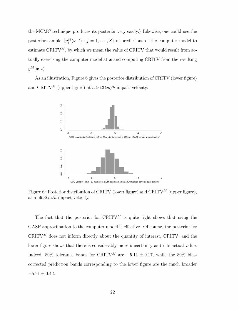
As an illustration, Figure 6 gives the posterior distribution of CRITV (lower figure)

and CRITVM (upper figure) at a 56.3km/h impact velocity.

-7 -6 -5 -4 -3

0.0

1.0

2.0

3.0

SDM velocity (km/h) 30 ms before SDM displacement is 125mm (GASP model approximation)

-7 -6 -5 -4 -3

0.0

0.4

0.8

1.2

SDM velocity (km/h) 30 ms before SDM displacement is 125mm (bias-corrected prediction)

Figure 6: Posterior distribution of CRITV (lower figure) and CRITVM (upper figure),at a 56.3km/h impact velocity.

The fact that the posterior for CRITVM is quite tight shows that using the

GASP approximation to the computer model is effective. Of course, the posterior for

CRITVM does not inform directly about the quantity of interest, CRITV, and the

lower figure shows that there is considerably more uncertainty as to its actual value.

Indeed, 80% tolerance bands for CRITVM are −5.11 ± 0.17, while the 80% bias-

corrected prediction bands corresponding to the lower figure are the much broader

−5.21 ± 0.42.

22

5 HIERARCHICAL MODELING FOR RELATED

SITUATIONS

In trying to extrapolate prediction to a new scenario in which only limited data is

available, one can use hierarchical modeling. Hierarchical modeling applies most di-

rectly to scenarios in which there are K different function outputs, to be denoted by

subscripts i, each coming from different configurations of a computer model (or even

from different computer models); in the CRASH example, these differing configura-

tions are the differing impact angles and barrier types. Related analyses can be found

in Han et al. (2009) and Higdon and Gattiker (2008). An alternative approach, using

multivariate Gaussian processes to directly model the multivariate outputs, can be

found in Qian et al. (2008) and in Conti and O’Hagan (2007).

Each of the different model configuration output functions can be modeled as was

done in sections 3 and 4, through Gaussian process priors. We will be particularly

concerned with settings where the Gaussian processes for yMi and bi can be assumed

to share common features, typically, where the parameters governing the priors are

drawn from a common distribution. This induces connections among the individual

models and enables us to combine information from the separate models, sharpen

analyses, and reduce uncertainties.

Implementation of these ideas will depend heavily on what data, both computer

and field, are available as well as the legitimacy of the assumptions imposed. Here, we

state and comment on these assumptions for the simplest structure we will impose,

leaving some of the details to Appendix C.

Assumption 1. The correlation parameters of the model approximation processes

are identical across the K configurations being considered; i.e., all computer model

and field data have common α’s and common β’s, which are assigned priors as in

23

the single-model case. This assumption was made because the CRASH data is too

limited to allow separate determination of the correlation parameters for each model

configuration, and the engineers involved in the study viewed the assumption as

reasonable. (The data is also too limited to provide any evidence that this assumption

might be incorrect.) In other contexts, this assumption may well be inadvisable.

Assumption 2. The variances 1/λM of the model approximation processes are

equal, across the various cases, as are the variances 1/λF of the field data. The priors

used for these parameters are as in the single-model case. If one had sufficient data,

relaxing this assumption (i.e., allowing differing variances following a hierarchical

model) would be natural (and likely more important than relaxing Assumption 1).

Assumption 3. The unknown mean parameters, µMi , of the GASP approximations

for the K computer model configurations, are assumed to arise from the two-stage

hierarchical model detailed in Appendix C. This prior distribution will allow the

computer model outputs to vary considerably between the K configurations, but still

ensures that information is appropriately pooled in their estimation.

Assumption 4. The bias process means, µb, are less important in the analysis than

the bias process precisions, λbi , so having the latter vary between model configurations

was felt to be allowing sufficient variation in the bias processes, given the limited

amount of available data. The bias process means for the K configurations are set

equal to a common (unknown) parameter µb with a prior as in the single-model case.

The variances of the bias processes are related in a fashion described by a parame-

ter q, whose value must be specified. Specifically, we assume that log(λbi) ∼ N(η, 4q2),

with specified q and a constant prior assigned to η. Parameter q describes the believed

degree of similarity in the biases for the K different computer model configurations;

indeed, 1 + q can be interpreted as an upper bound on the believed ratio of the stan-

24

dard deviations of the biases, or, stated another way, the proportional variation in

the bias is q. For instance, q = 0.1 implies that the biases are expected to vary by

about 10% among the various cases being considered.

Note that specification of q is a judgment as to the comparative accuracy of the

K different computer model configurations, as opposed to their absolute accuracy

(which need not be specified). The reason we require specification of q by the engi-

neer/scientist is that there is typically very little information about this parameter

in the data (unless K is large). Specifying q to be zero could be reasonable, if one is

unsure as to the accuracy of the computer models but is quite sure that the accuracies

are the same across the various K.

Finally, the correlation parameters of the bias processes are assumed to be common

across the K different configurations, and are assigned priors as in the single-model

case; in particular, the smoothness parameters are set equal to 2.

The analysis reported in Section 4 was for the data and model for rigid barrier,

straight frontal impact. By use of hierarchical modeling we can simultaneously treat

rigid barrier, left angle and right angle impacts as well as center pole impact. Thus

we use the hierarchical model with K = 4 related situations. The analyses and

predictions reported below are for a 56.3km/h impact (this is at the high end of

the data). The hierarchical model was used with q = 0.1. For simplicity, however,

the prior distributions used for the GASP parameters were chosen to be the same

as those used for the straight frontal analysis (and described in Appendix A); this

is reasonable, since the priors are relatively non-informative and the straight frontal

dataset is by far the largest of the four categories.

Figure 7 shows the posterior distributions of log(λbi) and µM

i for individual barrier

types. Note that, while the assumed similarity between the models allows information

to be passed from ‘large data’ to ‘small data’ models, the models are still allowed to

vary significantly.

25

-1.4 -1.2 -1.0 -0.8 -0.6

01

23

45

6

0.2 0.4 0.6 0.8 1.0 1.2 1.4

01

23

-1.4 -1.2 -1.0 -0.8 -0.6

01

23

45

6

0.2 0.4 0.6 0.8 1.0 1.2 1.4

01

23

4

-1.4 -1.2 -1.0 -0.8 -0.6

01

23

45

0.2 0.4 0.6 0.8 1.0 1.2 1.4

01

23

45

6

-1.4 -1.2 -1.0 -0.8 -0.6

01

23

45

0.2 0.4 0.6 0.8 1.0 1.2 1.4

0.0

0.5

1.0

1.5

2.0

2.5

left

angl

est

raig

ht fr

onta

lrig

ht a

ngle

cent

er p

ole

PSfrag

replacem

ents

µMi log(λb

i)

Figure 7: Posterior distributions of µMi and log(λb

i) for the 4 barrier types, based onthe hierarchical model.

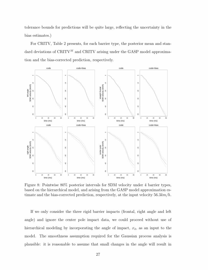
Figure 8 shows the differing posterior predictive SDM velocity curves and point-

wise uncertainty bands for each of the four barrier types. The straight frontal and

left angle posterior intervals in Figure 8 are tight, in part because there are data with

inputs close to 56.3km/h for these barrier types. In contrast, the intervals are not

tight for the other two barrier types because data near 56.3km/h are lacking. (This

thus reinforces the potential value of making a model run at a new desired input.)

Note that Figure 5 and the straight frontal pictures in Figure 8 are similar, so that

the hierarchical analysis did not greatly affect the answers for this barrier type.

Figure 9 gives the estimates of the four bias functions and the associated pointwise

uncertainties. Because of the large uncertainties in the bias estimates, the only case

in which the bias seems clearly different from zero is for left angle impacts, after

43ms. (While we cannot clearly assert that there is bias in the other cases, the

26

tolerance bounds for predictions will be quite large, reflecting the uncertainty in the

bias estimates.)

For CRITV, Table 2 presents, for each barrier type, the posterior mean and stan-

dard deviations of CRITVM and CRITV arising under the GASP model approxima-

tion and the bias-corrected prediction, respectively.

0 20 40 60 80

-50

-40

-30

-20

-10

0

code

0 20 40 60 80

-50

-40

-30

-20

-10

0

code+bias

left

angl

eS

DM

vel

ocity

(km

/h)

time (ms) time (ms)

0 20 40 60 80

-50

-40

-30

-20

-10

0

code

0 20 40 60 80

-50

-40

-30

-20

-10

0

code+bias

stra

ight

fron

tal

SD

M v

eloc

ity (

km/h

)

time (ms) time (ms)

0 20 40 60 80

-50

-40

-30

-20

-10

0

code

0 20 40 60 80

-50

-40

-30

-20

-10

0

code+bias

right

ang

leS

DM

vel

ocity

(km

/h)

time (ms) time (ms)

0 20 40 60 80

-50

-40

-30

-20

-10

0

code

0 20 40 60 80

-50

-40

-30

-20

-10

0

code+bias

time (ms) time (ms)

cent

er p

ole

SD

M v

eloc

ity (

km/h

)

Figure 8: Pointwise 80% posterior intervals for SDM velocity under 4 barrier types,based on the hierarchical model, and arising from the GASP model approximation es-timate and the bias-corrected prediction, respectively, at the input velocity 56.3km/h.

If we only consider the three rigid barrier impacts (frontal, right angle and left

angle) and ignore the center pole impact data, we could proceed without use of

hierarchical modeling by incorporating the angle of impact, x2, as an input to the

model. The smoothness assumption required for the Gaussian process analysis is

plausible: it is reasonable to assume that small changes in the angle will result in

27

time (ms)

SD

M v

eloc

ity (

km/h

)

0 20 40 60 80

-4-2

02

4

left angle bias

time (ms)

SD

M v

eloc

ity (

km/h

)

0 20 40 60 80

-4-2

02

4

straight frontal bias

time (ms)

SD

M v

eloc

ity (

km/h

)

0 20 40 60 80

-4-2

02

4

right angle bias

time (ms)S

DM

vel

ocity

(km

/h)

0 20 40 60 80

-4-2

02

4

center pole bias

Figure 9: Estimates and pointwise 80% posterior intervals for bias, under 4 barriertypes, based on the hierarchical model and at the input velocity 56.3km/h.

Hierarchical model Using frontal data onlyBarrier type CRITVM CRITV CRITVM CRITV

left angle -6.08 (0.34) -6.34 (0.49)straight frontal -5.13 (0.13) -5.22 (0.30) -5.11 (0.13) -5.21 (0.33)

right angle -6.89 (0.65) -6.80 (0.96)center pole -6.55 (0.74) -6.54 (0.91)

Table 2: Posterior mean and standard deviation of CRITVM and CRITV, at theinput velocity 56.3km/h.

small changes in the velocity-time curve so that yM is a smooth function of x2. We

performed this analysis with the input vector now being x = (x1, x2), but the results

differed little from the results in the hierarchical analysis and so are not reported.

The computation was also considerably more intensive via this route.

6 FORMAL TESTING OF MODEL VALIDITY

A question often asked in the computer model validation community is “Is the com-

puter model correct?” While an increasing segment of the community understands

28

that the answer is ‘no,’ it is of considerable pedagogical interest to provide methodol-

ogy for clear demonstration of the answer. Bayesian testing (in which bias is allowed)

seems to be extremely powerful in addressing this question formally, and the goal of

this section is to present the relevant Bayesian testing methodology.

Letting M0 denote the computer model, a natural way to approach the question

is to formally test the hypothesis H : “M0 is true”. To test this hypothesis within the

Bayesian framework, an alternative model is needed. Luckily, we have a ready-made

alternative, M1, namely the model constructed in sections 3 and 4, which includes

the bias term b(x, t). To perform the test, we thus need only compute the posterior

probability that M0 is correct.

Let φi be the entire parameter vector for model Mi, i = 0, 1 (including all pa-

rameters of the mean functions and the Gaussian processes involved). In addition,

for model Mi, i = 0, 1, denote by fi(y | φi), pi(φi), and pi(φi | y) the likelihood

function of the full data vector y (both computer model and field data), the prior

density, and the posterior density for the parameter vector, respectively. The form of

the likelihood function and the approaches for prior specification and posterior infer-

ence, using MCMC methods, for model M0 are similar to the corresponding ones for

model M1, described earlier and detailed in appendices A and B, with one exception.

Use of improper priors is typically not possible when interest lies in computation of

the posterior probability of models. This is a potential concern because the Bayesian

predictive analysis discussed previously assigned constant improper priors to both

µM and µb. However, the parameter µM is a location-parameter that occurs in both

models and so can be assigned the constant prior, as justified in Berger et al. (2001).

Unfortunately, µb only occurs in model M1, and so it cannot be assigned a con-

stant prior. Hence, for the computation in this section, we simply assumed that

µb = 0.

Letting π1 = 1 − π0 denote the prior probability of model M1, Bayes theo-

29

rem yields that the posterior probability of model M0 is given by P (M0 | y) =

π0m0(y)/[π0m0(y) + π1m1(y)], where

mi(y) =

∫

fi(y | φi)pi(φi)dφi (6.1)

is the marginal likelihood for model Mi, i = 0, 1.

Although we can analytically integrate in (6.1) over part of the parameter vector

φi, part of the integration must be done numerically. There are a variety of possible

methods for such numerical integration (see, e.g., Han and Carlin (2001)). We con-

sidered two approaches: that of Chib and Jeliazkov (2001); and importance sampling,

utilizing a t distribution (with mean and variance estimated from the MCMC output)

as the importance function (see Bayarri et al. (2005) for the details).

For π0 = 1/2, the two computational approaches lead to posterior probabilities

for model M0 of 2.694× 10−26 and 1.334× 10−23, respectively. The computation via

importance sampling was stable and accurate (which is easy to assess because the

importance samples are i.i.d.), but the computation using the method of Chib and

Jeliazkov did not seem to fully stabilize; the convergence process appears to have very

heavy tails.

Finally, it should be mentioned that it is often more reasonable to approach formal

testing of validity by simply testing if the bias is suitably small, say, |b(x, t)| < δ for

all t in an interval of interest, and for some specified δ. This could easily be done

using the posterior samples of the bias, as in Section 4.2.1.

30

7 SUMMARY

7.1 Conclusions for CRASH and Engineering

The basic question of interest to the engineers in the study was whether CRASH reli-

ably reproduces the results of physical tests of vehicle crashworthiness. It was found

that CRASH is reasonably reliable (with quantified uncertainty) for larger impact

velocities, but has a definite bias at lower impact velocities. This was of consider-

able interest and intiated a re-examination of the computer model to determine the

source of this bias. The development of the bias-corrected prediction methodology

for CRASH also allowed use of the current CRASH model, in spite of the bias.

The quantity CRITV was of particular importance for the users of the code, as

it related to air bag firing times. Using the bias-corrected prediction methodology, it

was not only possible to estimate CRITV, but also to assess the uncertainty in the

estimate (crucial for a design issue as sensitive as air bag firing); such uncertainties

were not previously available.

The emulator of the computer model that was constructed, as part of the analysis,

was also found to be very useful for exploring the design space in a much more efficient

way than could the CRASH model itself (due to the prohibitive run-times of CRASH).

Finally, this case-study was an important step in the development of a general

set of tools that are now being used by engineers in the validation of a variety of

computer models constructed for vehicle design.

7.2 Summary of Technical Innovations

The methodological extensions of the framework described in Bayarri et al. (2007b),

to meet the challenges imposed by the problem of validating the CRASH model,

are potentially useful for other applications that involve (time-dependent) functional

data that are suitably smooth. By discretizing the model output and field curves at

31

a relatively small number of time points, it is possible to incorporate functional data

by the direct method of treating time as an additional input to the model and field

processes. To overcome the computational issues that could result from the explosion

of input values, a strategy based on a Kronecker product formulation of the covariance

matrices was introduced. To be computationally successful, the strategy requires

that the various Gaussian processes used in the analysis have a common correlation

structure in terms of time. (While this assumption is plausible for the CRASH model,

it is certainly an assumption to be considered carefully in other applications.)

A further methodological contribution was the way of incorporating constraints –

such as the restriction that relative velocities are zero at time zero – into the analysis.

The CRASH dataset comprises limited data regarding impact configurations other

than the straight frontal. Another technical innovation was thus to construct a hi-

erarchical model that is able to appropriately borrow strength across the different

configurations. Strong assumptions were required but, in such data-limited situa-

tions, there is no real alternative.

Finally, a method was developed for formally testing the hypothesis that the

computer model is an adequate representation of reality, although we argued that

such tests are of limited utility.

SUPPLEMENTAL MATERIALS

Technical Report: “NISS-tech-report-163.pdf” is the Bayarri et al. (2005) National

Institute of Statistical Sciences technical report, referenced in Sections 1.5 and

6, and Appendixes B and C. (pdf file)

32

References

Bayarri, M., Berger, J., Cafeo, J., Garcia-Donato, G., Liu, F., Palomo, J.,Parthasarathy, R. J., Paulo, R., Sacks, J., and Walsh, D. (2007a), “Computermodel validation with functional output,” Annals of Statistics, 35, 1874–1906.

Bayarri, M. J., Berger, J. O., Kennedy, M., Kottas, A., Paulo, R., Sacks, J., Cafeo,J. A., Lin, C. H., and Tu, J. (2005), “Bayesian Validation of a Computer Model forVehicle Crashworthiness,” Tech. Rep. 163, National Institute of Statistical Sciences,available at http://pubs.amstat.org/loi/jasa.

Bayarri, M. J., Berger, J. O., Paulo, R., Sacks, J., Cafeo, J. A., Cavendish, J., Lin,C. H., and Tu, J. (2007b), “A framework for validation of computer models,”Technometrics, 49, 138–154.

Berger, J. O., De Oliveira, V., and Sanso, B. (2001), “Objective Bayesian analysisof spatially correlated data,” Journal of the American Statistical Association, 96,1361–1374.

Bernardo, C., Buck, R., Liu, L., Nazaret, W., Sacks, J., and Welch, W. (1992), “Inte-grated circuit design optimization using a sequential strategy,” IEEE Transactionson Computer-Aided Design, II., No. 3.

Campbell, K. (2006), “Statistical calibration of computer simulation,” Reliability En-gineering & System Safety, 91, 1358–1363.

Chib, S. and Jeliazkov, I. (2001), “Marginal likelihood from the Metropolis-Hastingsoutput,” Journal of the American Statistical Association, 96, 270–281.

Conti, S. and O’Hagan, A. (2007), “Bayesian emulation of complex mul-tioutput and dynamic computer models,” Tech. Rep. 569/07, Depart-ment of Probability and Statistics, University of Sheffield, available athttp://www.tonyohagan.co.uk/academic/ps/multioutput.ps.

Craig, P. S., Goldstein, M., Rougier, J. C., and Seheult, A. H. (2001), “Bayesian fore-casting for complex systems using computer simulators,” Journal of the AmericanStatistical Association, 96, 717–729.

Craig, P. S., Goldstein, M., Seheult, A. H., and Smith, J. A. (1997), “Pressure match-ing for hydrocarbon reservoirs: a case study in the use of Bayes linear strategies forlarge computer experiments,” in Case Studies in Bayesian Statistics: Volume III.Gatsonis, C., Hodges, J. S., Kass, R. E., McCulloch, R., Rossi, P. and Singpur-walla, N. D. (eds.), pp. 36–93.

Currin, C., Mitchell, T., Morris, M., and Ylvisaker, D. (1991), “Bayesian predictionof deterministic functions, with applications to the design and analysis of computerexperiments,” Journal of the American Statistical Association, 86, 953–963.

33

Gelman, A., Carlin, J. B., Stern, H. S., and Rubin, D. B. (1995), Bayesian dataanalysis, Chapman & Hall Ltd.

Goldstein, M. and Rougier, J. C. (2003), “Calibrated Bayesian forecasting using largecomputer simulators,” Tech. rep., Statistics and Probability Group, University ofDurham.

— (2004), “Probabilistic formulations for transferring inferences from mathematicalmodels to physical systems,” SIAM Journal on Scientific Computing, 26, 467–487.

Goldstein, M. and Wooff, D. A. (2007), Bayes Linear Statistics: Theory & Methods,Jonh Wiley & Sons.

Gramacy, R. and Lee, H. (2006), “Adaptive design of supercomputer experiments,”Tech. Rep. AMS2006–13, UCSC Department of Applied Math and Statistics.

— (2008), “Bayesian treed Gaussian process models with an application to computermodeling,” Journal of the American Statistical Association, 103, 1119–1130.

Han, C. and Carlin, B. (2001), “Markov chain Monte Carlo methods for computingBayes factors: a comparative review,” Journal of the American Statistical Associ-ation, 96, 1122–1132.

Han, G., Santner, T. J., Notz, W. I., and Bartel, D. L. (2009), “Prediction for com-puter experiments having quantitative and qualitative Input Variables,” Techno-metrics, to appear.

Higdon, D. and Gattiker, J. (2008), “Comment on Article by Sanso et al.” BayesianAnalysis, 3, 39–44.

Higdon, D., Gattiker, J., and Willians, B. (2008), “Computer model calibration usinghigh dimensional output,” Journal of the American Statistical Association, 103,570–583.

Higdon, D., Kennedy, M. C., Cavendish, J., Cafeo, J., and Ryne, R. D. (2004),“Combining field data and computer simulations for calibration and prediction,”SIAM Journal on Scientific Computing, 26, 448–466.

Kennedy, M. C. and O’Hagan, A. (2001), “Bayesian calibration of computer models(with discussion),” Journal of the Royal Statistical Society B, 63, 425–464.

Kennedy, M. C., O’Hagan, A., and Higgins, N. (2002), “Bayesian analysis of computercode outputs,” in Quantitative Methods for Current Environmental Issues. C. W.Anderson, V. Barnett, P. C. Chatwin, and A. H. El-Shaarawi (eds.), Springer-Verlag: London, pp. 227–243.

Lee, H., Sanso, B., Zhou, W., and Higdon, D. (2006), “Inferring particle distributionin a proton accelerator experiment,” Bayesian Analysis, 1, 249–264.

34

McFarkand, J., Mahadevan, S., Romero, V., and Swiler, L. (2008), “Calibration anduncertainty analysis for computer simulations with multivariate output,” AIAAJournal, 46, 1253–1265.

Morris, M. D., Mitchell, T. J., and Ylvisaker, D. (1993), “Bayesian design and analysisof computer experiments: Use of derivatives in surface prediction,” Technometrics,35, 243–255.

Oberkampf, W. and Trucano, T. (2000), “Validation Methodology in ComputationalFluid Dynamics,” Tech. Rep. 2000-2549, American Institute of Aeronautics andAstronautics.

Paulo, R. (2005), “Default priors for Gaussian processes,” Annals of Statistics, 33,556–582.

Pilch, M., Trucano, T., Moya, J. L., Froehlich, G. Hodges, A., and Peercy, D. (2001),“Guidelines for Sandia ASCI Verification and Validation Plans - Content and For-mat: Version 2.0,” Tech. Rep. SAND 2001-3101, Sandia National Laboratories.

Qian, P. Z. G., Wu, H., and Wu, C. F. J. (2008), “Gaussian Process Models for Com-puter Experiments with Qualitative and Quantitative Factors,” Technometrics, 50,383–396.

Roache, P. (1998), Verification and Validation in Computational Science and Engi-neering, Albuquerque: Hermosa Publishers.

Robert, C. and Casella, G. (2004), Monte Carlo Statistical Methods, Second Edition,New York: Springer.

Rougier, J. (2007), “Efficient emulators for multivariate deterministic functions,”Tech. rep., Department of Mathematics, University of Bristol.

Sacks, J., Welch, W. J., Mitchell, T. J., and Wynn, H. P. (1989), “Design and analysisof computer experiments (C/R: p423-435),” Statistical Science, 4, 409–423.

Santner, T., Williams, B., and Notz, W. (2003), The Design and Analysis of ComputerExperiments, Springer-Verlag.

Stein, M. (1999), Statistical Interpolation of Spatial Data: Some Theory for Kriging,New York: Springer.

Trucano, T., Pilch, M., and Oberkampf, W. O. (2002), “General Concepts for Ex-perimental Validation of ASCII Code Applications,” Tech. Rep. SAND 2002-0341,Sandia National Laboratories.

Welch, W. J., Buck, R. J., Sacks, J., Wynn, H. P., Mitchell, T. J., and Morris,M. D. (1992), “Screening, predicting, and computer experiments,” Technometrics,34, 15–25.

35

Williams, B., Higdon, D., Gattiker, J., Moore, L., McKay, M., and Keller-MacNulty,S. (2006), “Combining experimental data and computer simulations, with an ap-plication to flyer plate experiments,” Bayesian Analysis, 1, 765–792.

Yang, R. and Chen, M. (1995), “Bayesian analysis for random coefficient regressionmodels using noninformative priors,” Journal of Multivariate Analysis, 55, 283–311.

A The Model

The Likelihood: Let µM(z) = Ψ(z)′µM be the mean of the Gaussian process

prior for the computer model, where Ψ(z) is an r-dimensional known function of z.

This general formulation includes as a special case the linear trend form used for the

CRASH model (and given in Section 3).

Given the unknown parameters, the data y = (yM ′

, yF ′

)′ is normally distributed

with mean vector Xθ and covariance matrix Σ⊗CT (DT , DT ) where θ = ((µM)′, µb)′,

X =

Ψ(z1)′ 0

......

Ψ(zm)′ 0

Ψ(z?1)

′ 1

......

Ψ(z?n)′ 1

, (A-1)

Σ =

1λM CM(DM , DM) 1

λM CM(DM , DF )

1λM CM(DM , DF )′ 1

λM CM(DF , DF ) + 1λb C

b(DF , DF ) + 1λF In×n

. (A-2)

Prior distributions: Since θ is a location vector, we utilize the standard constant

prior density p(θ) = 1. It thus remains only to specify the prior density for ξ =

(λM , λb, λF , βM , βb, βT , αM , αT ).

36

For the smoothness parameters αM and αT , we choose uniform priors on their

ranges (each α` being in the interval (1, 2)). The precision parameters (λM , λb, λF )

and range parameters (βM` , βb

` , βT ) are given independent exponential priors, with

means set at 10 times the marginal likelihood estimate of the parameter. This was

essentially an empirically driven choice. When the mean was set at 10 times the

marginal MLE, the prior had little influence on the answer (so that the ‘double use’

of the data in defining the centering of the prior is not a significant sin), and the

exponential tail did help considerably with the convergence of the MCMC.

The marginal MLE of ξ is defined as the MLE from the integrated likelihood,

obtained by integrating out θ with respect to its prior. Explicit formulas for this

integrated likelihood, for the associated Fisher information matrix, and details about

the utilization of Fisher’s scoring method in computing the estimate can be found in

Berger et al. (2001) and Paulo (2005).

In the CRASH application, the marginal MLE of (λM , λb, λF , βT , βM , βb) is

(0.051, 0.77, 1.24, 2.63, 0.25, 31.7), and hence the prior on, e.g., βT is an exponential

distribution with mean 10 × 2.63. The marginal MLEs for αT and αM are, respec-

tively, 1.10 and 1.03 (recall that αb was fixed at 2), but these are not used in the prior

specification since these parameters are a priori uniform on their ranges.

B Monte Carlo methods for posterior inference

Generating samples from the posterior distribution of the unknown param-

eters: The form of covariance matrix Σ⊗CT (DT , DT ) does not result in simple ex-

pressions for full conditional distributions of parameters contained in ξ, so we utilized

a block Gibbs sampler to generate from the posterior distribution. We work with two

full conditionals, p(θ | ξ, y) and p(ξ | θ, y), and, given the current draw (θ(old), ξ(old)),

update according to (a) θ(new) ∼ p(θ | ξ(old), y); and (b) ξ(new) ∼ p(ξ | θ(new), y). Step

37

(a) is easily implemented since p(θ | ξ, y) is a multivariate normal density with mean

vector (X ′(Σ⊗CT (DT , DT ))−1X)−1X ′(Σ⊗CT (DT , DT ))−1y and covariance matrix

(X ′(Σ ⊗ CT (DT , DT ))−1X)−1.

To sample from p(ξ | θ, y), we use a Metropolis-Hastings algorithm (e.g., Robert

and Casella (2004)). To facilitate the choice of the proposal distribution, we transform

ξ to ξ? = g(ξ), where

g(ξ) =

(

ln[(λM , λb, λF , βM ′

, βb′, βT )′], ln

(

αM − 1

2 − αM

)

, ln

(

αT − 1

2 − αT

))

and the operations involving vectors should be interpreted componentwise.

A proposal distribution with which we have had good empirical results arises from

a t-density with ν degrees of freedom, centered at g(ξ(old)), and with scale matrix

proportional to I−1(ξ?). Here, ξ? is the (marginal) MLE for ξ?, obtained from the

(marginal) MLE ξ for ξ, and I(ξ?) is the estimated information matrix, obtained

from I(ξ), the corresponding matrix for ξ (both discussed in Appendix A). Note

that the actual proposal distribution for ξ is induced by the multivariate t proposal

for ξ?, through the transformation g, and is not symmetric. To choose the constant

c to multiply I−1(ξ?), we can start by trying c = 2.4/√

d, where d is the dimension

of ξ, as suggested by Gelman et al. (1995), and then increasing or decreasing c in

order to achieve a suitable acceptance rate. For CRASH, good mixing was achieved

for ν = 5 and c = 1.5.

Simulating realizations from the posterior distribution of functions: One

usually wants to predict functions such as yM(x, t), yR(x, t) and b(x, t) at a finer set of

t values than DT . This is possible because the computations involved in prediction are

much faster than those involved in obtaining a posterior sample of unknown param-

eters. Thus suppose prediction is desired at the nP time points DPt = t1, . . . , tnP

.

(Note that Kronecker product simplifications will not then be possible, but that is

38

not a problem here.) If prediction is desired at input x, it follows that we need to

predict the functions at the combined inputs DP = (x, t1), . . . , (x, tnP).

Hence, we need to generate a sample from the posterior predictive distribution of

the combined vector r(DP ) = (yM(DP )′, b(DP )′)′, where yM(DP ) and b(DP ) denote

the vectors of sampled yM and b function points respectively. Conditional on (θ, ξ),

the joint distribution of r(DP ) and the data is multivariate normal with readily

computed mean and covariance vectors. The conditional distribution for r(DP ) is

therefore easy to obtain as well. Hence, to draw a sample from the desired posterior

predictive distribution, for every MCMC sample (θj, ξj), we only need to draw from

the ensuing conditional multivariate normal.

The results reported for CRASH were based on MCMC posterior samples obtained

by discarding the first 10,000 iterations (burn-in), storing the next 40,000 sampled

values, and selecting every 40th point from this collection. The resulting 1,000 pos-

terior samples for the parameters were then used to generate 1,000 realizations of

yM(x, t) and b(x, t) at the inputs x of interest, for t in DPt = 3, 6, . . . , 81.

Updating: The model approximation is exact only at the observed model-run data

points. Sometimes the values of the model output are also constrained at other points.

For instance, in CRASH, all relative velocity curves are (by definition) equal to zero

at t = 0. If one tried to incorporate this constraint a priori , the Kronecker prod-

uct computational simplification would no longer apply, resulting in an impractical

MCMC algorithm. Another crucial instance of the conditioning idea is when an ad-

ditional computer model run, yM(x, t), becomes available. Indeed, this is how the

computer model is often utilized for a new input x of interest. The difficulty here is

that it may not be feasible to re-run the entire MCMC algorithm with this new data

point.

The solution to both these problems is simply to condition the existing poste-

39

rior on the additional constraint or data point; i.e., use the additional informa-

tion in the Kalman filter part of the analysis, but not to obtain the posterior for

tuning parameters or parameters in the Gaussian processes. To illustrate this ap-

proach, consider updating the posterior by the constraint that the relative velocity

is 0 at t = 0. This is equivalent to introducing the ‘new (extended) observations’

yM(x1, 0) = yR(x1, 0) = 0. Let Σ+ denote the prior covariance matrix of the new

data vector y+ = (y′, yM(x1, 0), yR(x1, 0))′. The Σ+ can be written in a block format

to take advantage of the already computed inverses for Σ and CT (DT , DT ), and of

the Kronecker structure. Posterior quantities can then be recalculated by replacing

(Σ ⊗ CT (DT , DT ))−1 by (Σ+)−1 and replacing y by y+. More details can be found

in Bayarri et al. (2005).

C Hierarchical model assumptions and analysis

Suppose we have K related models. For the ith model, we use the subscript i for the

parameters µM , and λb that are allowed to vary between models. The assumptions

made in the hierarchical analysis are as follows.

1. All models and field data have common α’s, common β’s, common µb’s, common

λM ’s, and common λF ’s, with priors as in Appendix A.

2. µMi | µ,Υ ∼ Nr(µ,Υ). (Recall that r is the dimension of the linear model

for the mean of the Gaussian process prior for the model output.) The hyper-

parameters µ and Υ are assigned a reference prior, written in terms of µ and

Ω = λMΥ, following Yang and Chen (1995). When r = 1 as for CRASH, so

that the hierarchical prior is µMi | µ, τ ∼ N(µ, τ−1), this reference prior can be

shown to be

p(µ, τ | λM , αM , βM , αT , βT ) =1

τ

∣

∣

∣

∣

∣

K∑

i=1

(

1 +τ

λMXMi C−1

i XM ′

i

)

−2∣

∣

∣

∣

∣

1/2

,

40

where XMi = (Ψ(zi1)

′, . . . , Ψ(zimi)′)′, and Ci = CM

i (DMi , DM

i )⊗CT (DT , DT ).

For the case of arbitrary r, see Bayarri et al. (2005).

3. log(λbi) ∼ N(η, 4q2); q needs to be specified, η is given a constant prior.

We note that the Monte Carlo methods described in Appendix B can be extended

to provide a simulation-based model fitting technique for the hierarchical model.

In terms of the MCMC, and restricting attention to the CRASH example, the full

conditionals of µMi , µb, µ, and η are Normal, and hence can be sampled directly.

The common parameters are sampled as a block, using a Metropolis-Hastings step

with a proposal similar to the one used in the single barrier analysis, except that now

λb is excluded from this step as it is not common across the different computer models.

To sample from the full conditional of the λbi and τ we follow a similar strategy: we

reparametrize in terms of the natural logarithms of these parameters and use a t

density proposal centered at the previous iteration and with a scale parameter that

needs to be tuned. See Bayarri et al. (2005) for the specifics of how the scales of these

proposals were tuned in the CRASH application.

41