
Predicting the yield curve using forecast combinations
38
Predicting the yield curve using forecast combinations Jo˜ao F. Caldeira a , Guilherme V. Moura b,1 , Andr´ e A. P. Santos b a Department of Economics Universidade Federal do Rio Grande do Sul & PPGA b Department of Economics Universidade Federal de Santa Catarina Abstract An examination of the statistical accuracy and economic value of modeling and forecasting the term structure of interest rates using forecast combinations is considered. Five alternative methods to combine point forecasts from several univariate and multivariate autoregressive specifications including dynamic factor models, equilibrium term structure models, and forward rate regression models are used. More- over, a detailed performance evaluation based not only on statistical measures of forecast accuracy, but also on Sharpe ratios of fixed income portfolios is conducted. An empirical application based on a large panel of Brazilian interest rate future contracts with different maturities shows that combined forecasts consistently outperform individual models in several instances, specially when economic criteria are taken into account. Keywords: yield curve, forecast combinations, economic value of forecasts 1. Introduction An interesting question still little-explored in the literature is the implementation and performance evaluation of forecast combinations for the yield curve. Existing evidence has focused on the performance evaluation of individual forecast models. However, combined forecasts has been extensively and success- fully applied in many areas; see Granger (1989), Clemen (1989), Granger & Jeon (2004), Timmermann (2006) and Wallis (2011) for reviews. Therefore, a natural question is: can forecast combinations deliver better forecasts for the yield curve? If so, are these forecasts economically relevant? The motivation to combine forecasts comes from an important result from the methodological liter- ature on forecasting, which shows that a linear combination of two or more forecasts may yield more accurate predictions than using only a single forecast (Granger, 1989; Newbold & Harvey, 2002; Aiolfi & Timmermann, 2006). Moreover, adaptive strategies for combining forecasts might also mitigate struc- tural breaks, model uncertainty and model misspecification, and thus lead to more accurate forecasts (Newbold & Harvey, 2002; Pesaran & Timmermann, 2007). In particular, there is recent evidence that combining forecast of nested models can significantly improve forecasting precision upon forecasts obtained from single model specifications (Clark & McCracken, 2009). Preprint submitted to Encontro Brasileiro de Finan¸ cas 2014 June 16, 2014
Transcript of Predicting the yield curve using forecast combinations

Predicting the yield curve using forecast combinations
Joao F. Caldeiraa, Guilherme V. Mourab,1, Andre A. P. Santosb
aDepartment of EconomicsUniversidade Federal do Rio Grande do Sul & PPGA
bDepartment of EconomicsUniversidade Federal de Santa Catarina
Abstract
An examination of the statistical accuracy and economic value of modeling and forecasting the term
structure of interest rates using forecast combinations is considered. Five alternative methods to combine
point forecasts from several univariate and multivariate autoregressive specifications including dynamic
factor models, equilibrium term structure models, and forward rate regression models are used. More-
over, a detailed performance evaluation based not only on statistical measures of forecast accuracy, but
also on Sharpe ratios of fixed income portfolios is conducted. An empirical application based on a large
panel of Brazilian interest rate future contracts with different maturities shows that combined forecasts
consistently outperform individual models in several instances, specially when economic criteria are
taken into account.
Keywords: yield curve, forecast combinations, economic value of forecasts
1. Introduction
An interesting question still little-explored in the literature is the implementation and performance
evaluation of forecast combinations for the yield curve. Existing evidence has focused on the performance
evaluation of individual forecast models. However, combined forecasts has been extensively and success-
fully applied in many areas; see Granger (1989), Clemen (1989), Granger & Jeon (2004), Timmermann
(2006) and Wallis (2011) for reviews. Therefore, a natural question is: can forecast combinations deliver
better forecasts for the yield curve? If so, are these forecasts economically relevant?
The motivation to combine forecasts comes from an important result from the methodological liter-
ature on forecasting, which shows that a linear combination of two or more forecasts may yield more
accurate predictions than using only a single forecast (Granger, 1989; Newbold & Harvey, 2002; Aiolfi &
Timmermann, 2006). Moreover, adaptive strategies for combining forecasts might also mitigate struc-
tural breaks, model uncertainty and model misspecification, and thus lead to more accurate forecasts
(Newbold & Harvey, 2002; Pesaran & Timmermann, 2007). In particular, there is recent evidence
that combining forecast of nested models can significantly improve forecasting precision upon forecasts
obtained from single model specifications (Clark & McCracken, 2009).
Preprint submitted to Encontro Brasileiro de Financas 2014 June 16, 2014

Hendry & Clements (2004) point out a number of potential explanations for the good performance of
combined forecasts vis-a-vis individual forecast models. First, if two models provide partial, but incom-
pletely overlapping explanations, then some combination of the two might do better than either alone.
Specifically, if two forecasts were differentially biased (one upwards, one downwards), then combining
could be an improvement over either. Similarly, if all explanatory variables were orthogonal, and models
contained subsets of these, an appropriately weighted combination could better reflect all the informa-
tion. Second, averaging forecasts reduces variance to the extent that separate sources of information are
used. Third, forecast combination can also alleviate the problem of model uncertainty. Finally, Granger
& Jeon (2004) point out that the benefits of pooling forecasts can be related to the portfolio selection
problem, since a portfolio of assets is usually better than investing in a single asset.
A large number of approaches to combine prediction models exist in the literature, ranging from sim-
ple averaging schemes to more sophisticated adaptive combinations. Various studies have demonstrated
that simple averaging of a multitude of forecasts works well in relation to more sophisticated weighting
schemes (Newbold & Harvey, 2002; Clark & McCracken, 2009). Timmermann (2006) argues that equal
weights are optimal in situations with an arbitrary number of forecasts when the individual forecast
errors have the same variance and identical pairwise correlations. More recently, Geweke & Amisano
(2011) study the properties of weighted linear combinations of prediction models (“linear pools”) by
using a predictive scoring rule. Among other results, the authors find that model weights depend on the
set of models analyzed, and models with positive weight in a larger pool may have zero weight if some
other models are deleted from that pool, thus indicating the importance of model complementarities for
forecasts.
The ability to forecast the behavior of the term structure of interest rates is important for macroe-
conomists, financial economists and fixed income managers. More specifically, bond portfolio optimiza-
tion, pricing of financial assets and their derivatives, as well as risk management, rely heavily on interest
rate forecasts. Moreover, these forecasts are widely used by financial institution, regulators, and in-
vestors to develop macroeconomic scenarios. However, until the seminal work of Diebold & Li (2006),
little attention was given to yield curve forecasting, and previous theoretical developments were mainly
focused on in-sample fit (see, for example, de Jong, 2000; Dai & Singleton, 2000). Diebold & Li (2006)
have taken an out-of-sample perspective based on a dynamic version of the static approach proposed by
Nelson & Siegel (1987) and have shown that this model produce accurate forecasts. The seminal work
of Diebold & Li (2006) on yield curve forecasting has been followed by a large number of studies that
investigate the performance of alternative forecasting models; see, for instance, Diebold & Rudebusch
(2013) for a text book review of these improvements.
The paper also provides a comprehensive evaluation of the performance of forecast combinations
vis-a-vis individual models in terms of both statistical accuracy and economic relevance, since the final
goal of interest rate forecasts is to improve economic and financial decision making. The existing
literature, however, has focused mainly on statistical measures of forecast accuracy, taking forecasts out
of the context in which they are ultimately used; see, for instance, de Pooter et al. (2010), Diebold &
2

Rudebusch (2013), and Caldeira et al. (2010), amongst others. As pointed out by Granger & Pesaran
(2000), Pesaran & Skouras (2002) and Granger & Machina (2006), when forecasts are used in decision
making, it is important to consider the decision process in the ex post evaluation of these forecasts,
maintaining the interaction between the forecasting model and the decision making task. Therefore, it
is of main concern to both academics and market practitioners the extent to which forecasts of interest
rates are useful to support economic decisions.
More specifically, we propose to evaluate the accuracy and economic relevance of yield curve forecasts
based on mean-variance optimal portfolios as introduced by Markowitz (1952). As a first step, we follow
Christoffersen & Diebold (1998), Hordahl et al. (2006), and de Pooter et al. (2010) and carry out
a traditional evaluation based on statistical measures of forecasting performance such as root mean
squared forecast error (RMSFE) and trace root mean squared forecast error (TRMSFE). In a second
step, different forecasts are used to construct mean-variance portfolios, which are then compared based
on their Sharpe ratios. In order to solve the mean-variance optimization problem, we use the different
forecasts to derive estimates of expected bond returns, and use these as inputs to obtain mean-variance
portfolios for alternative levels of risk tolerance.
We obtain forecasts of the yield curve based on a broad set of alternative models usually considered
in the literature. First, we consider a class of purely statistical models such as the random walk, the
univariate autoregressive model, the vector autoregressive and the Bayesian vector autoregressive model.
Second, we consider the class of yield curve factor models such as the dynamic versions of the Nelson-
Siegel and Svensson specifications. Third, we implement three alternative specifications that exploit the
predictive power of the forward rates such as the slope regression suggested by Diebold & Li (2006),
and the forward rate regressions of Fama & Bliss (1987) and Cochrane & Piazzesi (2005). Finally,
we consider the three-factor equilibrium term structure model proposed by Cox et al. (1985b). More
importantly, we combine models from different classes via five alternative combination schemes. First,
we consider the case of equally weighted forecasts. Second, we consider the thick modeling approach
proposed by Granger & Jeon (2004) which consists of selecting the best forecasting models in the sub-
sample period for model evaluation, according to the root mean square error (RMSE) criterion. In this
case, we use the selection process of Granger and Jeon and subsequently compute weights by means of
OLS regressions. Third, we use the rank-weighted combinations suggested by Aiolfi & Timmermann
(2006). Finally, we follow Morales-Arias & Moura (2013) and implement the thick modeling approach
with MSE-frequency and RMSE-frequency weights, which consists of selecting models by means of the
thick-modeling approach and assigning to each individual forecast a weight equal to a model’s empirical
frequency of minimizing the MSE and RMSE, respectively, over realized forecasts.
Our paper adds to the existing literature on yield curve forecasting in at least two aspects. First,
de Pooter et al. (2010) consider the problem of forecast combination for the yield curve using only equal
weights and MSFE-based weighting, and focus on the importance of macro variables in forecasting the
yield curve. We, on the other hand, consider a richer set of forecast combination schemes. Second,
Carriero et al. (2012) also consider the problem of economic evaluation of the term structure forecasts.
3

Our paper, however, takes this evaluation criterion and extends to the case of forecast combination
involving several individual models. Moreover, our paper differs in several important aspects with
respect to the few previous studies that address the question regarding the economic evaluation of
yield curve forecasts. First, the data set used in this paper carries interesting characteristics, since
it refers to a different marketplace, is sampled on a daily basis, and consists of high-liquidity fixed
income future contracts that resembles zero-coupon bonds. Second, Carriero et al. (2012) consider
trading strategies based only on one-step-ahead forecasts, whereas in our paper we consider the Sharpe
ratios from optimal portfolios based on multi-step-ahead forecasts including 1-week-, 1-month-, 2-month-
, and 3-month-ahead forecasts. Third, Carriero et al. (2012) obtain optimal mean-variance portfolio
weights considering a single value for the risk aversion coefficient, whereas we provide results considering
alternative levels of risk tolerance. Fourth, and most importantly, neither Carriero et al. (2012) nor
Xiang & Zhu (2013) provide results regarding the statistical differences in the Sharpe ratios of the
proposed approach with respect to the benchmark. We, on the other hand, employ a robust test for the
Sharpe ratio based on the bootstrap procedure of Ledoit & Wolf (2008), which allows us to formally
compare models in terms of an economic criterion. Fifth, none of the existing references focus on the
performance of forecast combinations. In this paper, however, we provide a comprehensive evaluation
by implementing five alternative forecast combination schemes, and check their performance in terms of
statistical accuracy and economic relevance.
Our empirical application is based on a large data set of constant-maturity future contracts of the
Brazilian Interbank Deposit (DI-futuro) which is equivalent to a zero-coupon bond and is highly liquid
(341 million contracts worth US$ 17.5 billion traded in 2012). The market for DI-futuro contracts
is one of the most liquid interest rate markets in the world. Many banks, insurance companies, and
investors use DI-futuro contracts as investment and hedging instruments. The data set considered in the
paper contains daily observations of DI-futuro contracts traded on the Brazilian Mercantile and Futures
Exchange (BM&FBovespa) with fixed maturities of 3, 6, 9, 12, 15, 18, 21, 24, 27, 30, 33, 36, 42 and 48
months. To obtain 1-week-, 1-month-, 2-month-, and 3-month-ahead forecasts for each of the maturities
available in the data set, we use individual forecasting models as well as alternative forecast combination
schemes. The results show that combined forecasts consistently outperform individual models in terms
of lower forecasting errors, and that this outperformance is more evident for shorter forecasting horizons.
Moreover, we also observe that the Sharpe ratios of the mean-variance portfolios built upon combined
forecasts are substantially and statistically higher than those obtained with the benchmark models. This
result is also robust to the level of risk tolerance and to the portfolio re-balancing frequency. Finally,
our results also suggest that, as long as yield curve forecasts are concerned, the differences in forecasting
performance among candidate models based on statistical criteria are also economic meaningful as they
generate optimal fixed income portfolios with improved risk-adjusted returns.
The paper is organized as follows. In Section 2 we describe the methods used to obtain forecasts
for the yield rates, including both individual forecast models as well as forecast combinations. Next, in
Section 3 we discuss the methodology used to evaluate forecast, both in terms of statistical criteria and
4

in terms of economic relevance. Section 4 brings an empirical application. Section 5 concludes.
2. Methods used to forecast the yield curve
In this section, we describe the methods used to forecast the yield curve. These methods are based
on individual forecast models as well as alternative forecast combinations.
2.1. Random walk model
The main benchmark model adopted in the paper is the random walk (RW), whose t+h-step-ahead
forecasts for an yield of maturity τ are given by:
yt+h(τ) = yt(τ) + εt(τ), εt(τ) ∼ N (0, σ2(τ)). (1)
In the RW, a h-step-ahead forecast, denoted yt+h(τ), is simply equal to the most recently observed
value yt(τ). This model is a good benchmark for judging the relative prediction power of other models,
since yields are usually nonstationary or nearly nonstationary. Thus, in practice, it is difficult to beat
the RW in terms of out-of-sample forecasting accuracy. Many other studies that consider interest rate
forecasting have shown that consistently outperforming the random walk is difficult (see, for example,
Duffee, 2002; Ang & Piazzesi, 2003; Diebold & Li, 2006; Hordahl et al. , 2006; Moench, 2008).
2.2. Univariate autoregressive model
It is possible to generalize the RW model and forecast the maturity-τ yield using a first-order uni-
variate autoregressive model (AR) that is estimated on the available data for that maturity:
yt(τ) = α + βyt−1(τ) + εt. (2)
The 1-step ahead forecast is produced as yt+1(τ) = α + βyt−1(τ). The forecasts for h-step ahead
horizon are obtained as:
yt+h|t(τ) = (1 + β + β2 + . . .+ βh−1)α + βhyt(τ).
2.3. Vector autoregressive model
The fact that the yield curve can be considered a vector process composed of yields of different
maturities indicates that the cross-section information might be important in understanding yield curve
movements. However, neither the RW nor the AR models exploit this information to build their forecasts.
Thus, a first-order unrestricted vector autoregressive model (VAR) for yield levels is a natural extension
of the univariate AR model. The estimated model is:
yt = A+Byt−1 + εt, (3)
5
where yt = (yt(τ1), yt(τ2), . . . , yt(τN))′. The 1-step ahead forecast is produced as yt = A + Byt−1, while
the h-step ahead forecasts are obtained as:
yt+h|t = (I + B + B2 + . . .+ Bh−1)A+ Bhyt. (4)
As argued by de Pooter et al. (2010), a well-known drawback of using an unrestricted VAR model
for yields is the large number of parameters that need to be estimated. Since our data set contains
thirteen different maturities, a substantial number of parameters needs to be estimated.
2.4. Bayesian vector autoregressive model
To alleviate the overparameterization of VARs without sacrificing completely the cross-section in-
formation as univariate models do, we follow Carriero et al. (2012) and use Bayesian VARs with a
Minnesota prior distribution (see Doan et al. , 1986; Litterman, 1986). Considering the vector autore-
gressive model in (3), this a priori belief implies that the expected value of matrix B is E [B] = δ × I.
We also need to determine how certain we are about our priori understanding, i.e. we need to set a
variance around the prior mean. It is assumed that B is conditionally normal, with first and second
moments given by:
E[Bij]
=
δi if i = j
0 if i 6= j, Var
[Bij]
= θσ2i
σ2j
, (5)
where (Bij) denotes the element in position (i, j) in matrix B, and where the covariance among the
coefficients in B are zero. Banbura et al. (2010) suggest to set δi = 1 for all i, reflecting the belief that
all the variables are characterized by high persistence. We believe it is reasonable to think a priori that
each of the yields obeys a univariate AR with high persistence, or equivalently, E [B] = 0.99 × I. The
hyperparameter θ controls the tightness of the prior, and the factor σ2i /σ
2j is a scaling parameter which
accounts for the different scale and variability of different maturities. Following Carriero et al. (2012),
we set the scale parameters σ2i equal to the variance of the residuals from a univariate autoregressive
model for the variables.
The prior specification is completed by assuming a diffuse normal prior on A and an inverted Wishart
prior for the matrix of disturbances Σ ∼ iW (ν0, S0), where ν0 and S0 are the prior scale and shape
parameters, and are set such that the prior expectation of Σ is equal to a fixed diagonal residual
variance Σ = diag (σ21, . . . , σ
2N).
We can re-write the VAR more compactly as:
Y = XΨ + E, (6)
where Y = [y2, . . . , yT ] is a (T − 1) × N matrix containing all the data points in yt, X = [1, Y−1] is a
(T −1)×M matrix containing a vector of ones (1) in the first columns and one lag of Y in the remaining
columns, Ψ = [A,B]′ is a M ×N matrix, and E = [ε1, . . . , εT ]′ is a (T − 1)×N matrix of disturbances.
6

As only one lag is considered we have M = N + 1. The Normal-Inverted Wishart prior has the form:
vec (Ψ) |Σ ∼ N (vec (Ψ0) ,Σ⊗ Ω0) , and Σ ∼ iW (ν0, S0), (7)
where the prior parameters Ψ0 Ω0, S0 and ν0 are chosen so that prior expectations and variances of Ψ
coincide with those implied by equation (5), E[Ψ] = Ψ0 and var[Ψ] = Σ ⊗ Ω0, where Σ is the variance
matrix of the disturbances and the elements of Ω0 are given by var [Bij] in (5). The conditional posterior
distribution of this model is also Normal-Inverted Wishart:
vec (Ψ) |Σ, Y ∼ N(Ψ,Σ⊗ Ω
), Σ|Y ∼ IW (ν, S), (8)
where the bar denotes parameters from the posterior distribution. Defining Ψ as the OLS estimates, we
have that Ψ = Ω(Ω−1
0 Ψ0 +X ′Y), Ω =
(Ω−1
0 +X ′X)−1
, ν = ν0 + T and S = S0 + Y ′Y + Ψ′0Ω−10 Ψ0 −
ΨΩ−1
Ψ. Since we are interested only in linear functions of the posterior moments of Ψ, the Appendix
A of Carriero et al. (2012) shows that it is possible to integrate Σ out of (8), yielding a matrix-variate
t marginal posterior distribution for Ψ:
Ψ|Y ∼Mt(Ψ,Ω−1, S, nu), (9)
whose expected value is given by Ψ = Ω(Ω−1
0 Ψ0 +X ′Y). To make explicit the link between Ψ and the
OLS estimates Ψ, we can use the normal equations to get:
Ψ = Ω(
Ω−10 Ψ0 +X ′XΨ
), (10)
which shows that Ψ is a weighted average of the prior mean and of the OLS estimates, where weights
are inversely proportional to their respective variances. Carriero et al. (2012) provide derivations of
these posterior moments in their Appendix A and Bauwens et al. (1999) present a text book treatment
of Bayesian VARs in their section 9.2 and deal explicitly with Minnesota priors in their subsection 9.2.3.
After computing Ψ, we can recover A and B, which allow us to obtain h-step ahead forecasts by
iteration:
Yt+h = A+ B · Yt+h−1, (11)
where Yt+h−1 is computed as in (4).
2.5. Models that exploit the predictive power of forward rates
We denote prices and log prices of a discount bond that promise to pay $1 at time t+ τ by Pt(τ) =
exp (−τ · yt(τ)) and pt(τ), respectively, and the yield of a τ -year bond by
yt(τ) = −1
τ· pt(τ). (12)
7

Once we have the yield curve, we can easily use it to derive the forward rates (see Piazzesi &
Schneider, 2009). The forward rate contracted at time t for loans from time t+ h to time t+ h+ τ can
be expressed as a linear function of yields with maturities τ + h and h:
fht (τ) =τ + h
τ· yt(τ + h)− h
τ· yt(h)
= yt(h) +τ + h
τ· (yt(τ + h)− yt(h)) . (13)
2.5.1. Fama-Bliss (FB) forward rate regression
The seminal work of Fama & Bliss (1987) examined the forecasting power in forward rates on the
same maturity excess return and provided an evidence against the expectations hypothesis in long-term
bonds. FB estimate a linear regression of the change in the τ -year bond yield on the forward-spot
spread,
yt+h(τ)− yt(τ) = αh(τ) + βh(τ)(fht (τ)− yt(τ)
), (14)
where fht (τ) is the forward rate contracted at time t for loans from time t+ h to time t+ h+ τ . Hence,
the h-step ahead forecasts yt+h(τ) are produced by projecting the changes in yields from time t to time
t+ h on the forward-spot at time t.
2.5.2. Cochrane-Piazzesi (CP) forward curve regression
Cochrane & Piazzesi (2005) find that the term structure of forward rates explains between 30% and
35% of the variation of bond excess returns over the same bond maturity spectrum investigated by FB.
Although the natural extension of this approach would imply putting all available forward rates on the
right side of the regression, we use only four forward rates (yt(12), f 12t (12), f 24
t (12), and f 36t (12)) to
avoid problems of multicolinearity, as suggested by Carriero et al. (2012). Then, we estimate a modified
version of equation (14), and forecasts are computed as follows:
yt+h(τ)− yt(τ) = αh + βh1 yt(12) + βh2 f12t (12) + βh3 f
24t (12) + βh3 f
36t (12). (15)
2.5.3. Slope regression
This model was used by Diebold & Li (2006) and is based on the historic spread between an yield on
a longer maturity bond and the yield on the shortest maturity bond. This difference is used to forecast
the change in the yield of the longer maturity bond. Specifically,
yt+h(τ)− yt(τ) = αh(τ) + βh(τ) (yt(τ)− yt(1)) , (16)
where yt(1) represents the 3 months yield, the shortest in our data set. The idea that the slope of the
yield curve reflects future movements in yields is, of course, not a new one and has its roots firmly in
the properties of the Expectations Hypothesis, wherein an upward sloping yield curve implies a future
8
rise in yields. This slope regression formulation is also closely related to, and uses almost the same
information, as the forward rate regressions of Fama & Bliss (1987), their generalization by Cochrane
& Piazzesi (2005), and the spread regressions of Campbell & Shiller (1991), which represent alternative
tests of the Expectations Hypothesis.
2.6. The 3-factor Cox, Ingersol & Ross Model (CIR) equilibrium model of the term structure
Cox et al. (1985b) developed one of the first general equilibrium theories of the term structure of
interest rates. Out of that theory came a model for pricing zero coupon bonds and derivatives. The
instantaneous nominal interest rate is assumed to be the sum of K = 3 state variables,
r =K∑j=1
yj,
and the state variable are assumed to be independent and generated as square root diffusion processes:
dyj = κj (θj − yj) + σj√yjdzj, for j = 1, . . . , K. (17)
The solution for the nominal price at time t of a nominally risk-free bond that pays $1 at time s is
determined as follows:
Pt(τ) = A1(τ) . . . AK(τ) · exp −B1(τ)y1t − . . .−BK(τ)ytK , (18)
where Aj(τ) and Bj(τ) have the form given in CIR:
Aj(τ) =
[2γe
12
(κj+λj−γj)τ
2γe−γjτ + (κj + λj + γj) (1− e−γjτ )
] 2κjθj
σ2j
, and (19)
Bj(τ) =2 (1− e−γjτ )
2γe−γjτ + (κj + λj + γj) (1− e−γjτ ), (20)
and γj =√
(κj + λj)2 + 2σ2j . Each state variable has a risk premium, λjyj, and each λj is treated as a
fixed parameter. The continuously compounded yield for a discount bond is defined as follows:
Rt(τ) = − logPt(τ)
τ, (21)
which is a linear function of the unobservable state variables. Given a set of yields on K discount bonds,
one can conceptually invert to infer values for the state variables. This inversion of bond rates to infer
values for the state variables has been used in Chen & Scott (1993), Duffie & Kan (1996), and Pearson
& Sun (1994). This model can be derived by applying arbitrage methods or by using the utility based
model as in Cox et al. (1985a). The risk premia are determined endogenously in a utility based model
by the co-variability of the state variables with marginal utility of wealth. The form for the risk premium
9
used here is consistent with a log utility model. To estimate the model we use the modified version of
the Kalman filter developed by Chen & Scott (2003).
2.7. Nelson-Siegel model class
Nelson & Siegel (1987) have shown that the term structure can be surprisingly well fitted at a
particular point in time by a linear combination of three smooth functions. The Nelson-Siegel model is
given by:
y(τ) = β1 + β2
(1− e−λτ
λτ
)+ β3
(1− e−λτ
λτ− e−λτ
)+ ετ , (22)
where β1 can be interpreted as the level of the yield curve, β2 as its slope, and β3 as its curvature. The
parameter λ determines the exponential decay of β2 and of β3.
Svensson (1994) proposed an extension of the original Nelson-Siegel model by adding an extra smooth
function to improve the flexibility and fit of the model. The model proposed by Svensson (1994) is
y(τ) = β1 + β2
(1− e−λ1τ
λ1τ
)+ β3
(1− e−λ1τ
λ1τ− e−λ1τ
)+ β4
(1− e−λ2τ
λ2τ− e−λ2τ
)+ ετ . (23)
Diebold & Li (2006) have introduced dynamics into the original Nelson-Siegel model, and showed
that its dynamic version has good forecasting power. The dynamic Nelson-Siegel model (henceforth
DNS) is given by:
yt(τ) = β1t + β2t
(1− e−λτ
λtτ
)+ β3t
(1− e−λτ
λτ− e−λτ
)+ εt(τ), (24)
where the vector of time-varying coefficients βt follow a VAR process.
Similarly to what Diebold & Li (2006) have done for the Nelson-Siegel model, a dynamic version of
Svensson model (hereafter DSV) can be written as:
yt(τ) = β1t + β2t
(1− e−λ1τ
λ1τ
)+ β3t
(1− e−λ1τ
λ1τ− e−λ1τ
)+ β4t
(1− e−λ2τ
λ2τ− e−λ2τ
)+ εt(τ). (25)
The fourth factor in the dynamic version of the Svensson model can be interpreted as a second curvature.
Svensson (1994) argues that the additional factor provides a better in-sample fit, especially for a richer
structure of yields, and therefore provides better estimations of forward rates.
The dynamic versions of both the Nelson-Siegel and Svensson models can be interpreted as dynamic
factor models (see, for example, Diebold et al. , 2006). More specifically, consider an N × T matrix of
observable yields. The observation at time t is denoted by yt = (y1t, . . . , yNt)′ , for t = 1, . . . , T , and yit
is ith variable in the vector yt at time t. The dynamic factor models considered are of the form
yt = Λ(λ)ft + εt, εt ∼ NID (0,Σ) , t = 1, . . . , T, (26)
10

where Λ(λ) is the N ×K matrix of factor loadings that depends on the decaying parameter λ, ft is a
K−dimensional vector containing the coefficients β1t, . . . , βKt for K = 3, 4, εt is the N × 1 vector of
disturbances and Σ is an N × N diagonal covariance matrix of the disturbances. The dynamic factors
ft are modeled by the following stochastic process:
ft = A+Bft−1 + ηt, ηt ∼ NID (0,Ω) , t = 1, . . . , T, (27)
where A is a K × 1 vector of constants, B is the K × K transition matrix, and Ω is the conditional
covariance matrix of disturbance vector ηt, which are independent of the residuals εt ∀t. Note that
equations (26) and (27) characterize a linear and Gaussian state space model and the Kalman filter can be
used to obtain the likelihood function via the prediction error decomposition. Here we follow Jungbacker
& Koopman (2008), who developed a simple transformation that generates significant computational
gains when the number of factors is smaller than the number of observed series (see Table 1 in Jungbacker
& Koopman, 2008, for an example of possible computational gains).
2.8. Combined forecasts
Assuming we are combining forecasts from M different forecast models, a combined forecast for a
h-month horizon for the yield with maturity τ is given by
yt+h|t(τ) =M∑m=1
wt+h|t,m(τ)yt+h|t,m(τ),
where wt+h|t,m(τ) denotes the weight assigned to the time-t forecast from the mth model, yt+h|t,m(τ).
Most of the forecast combination schemes considered are adaptive, meaning that the forecasts included
inM : yt+h|t,m(τ) and/or corresponding weights mth are based on alternative selection criteria within
a sub-sample of realized observations.
It is worth noting that since a forecaster would only have information available up to the fore-
cast origin ω, the sub-sample for forecast selection and computation of weights must contain data
on or before that period. Thus, we start by setting equal weights to all forecasts until the selec-
tion of forecasts and weighting schemes could be based on the evaluation of realized forecast er-
rors. This procedure guarantees that we use only information available up to a particular period
ω to set weights of forecasts for period ω + h. The following 5 alternative combination strategies
M = FC-EW,FC-OLS, FC-RANK,FC-MSE,FC-RMSE = 1, 2, . . . , 5 are considered:
1. Equally weighted forecasts (FC-EW): Various studies have demonstrated that simple averaging of
a multitude of forecasts works well in relation to more sophisticated weighting schemes (Newbold
& Harvey, 2002; Clark & McCracken, 2009). Therefore, the first forecast combination method we
consider assigns equal weights to the forecasts from all individual models, i.e. wt+h|t,m(τ) = 1/Mfor m = 1, . . . ,M. We denote the resulting combined forecast as Forecast Combination - Equally
11

Weighted (FC-EW). As explained in Timmermann (2006), this approach is likely to work well if
forecast errors from different models have similar variances and are highly correlated.
2. Thick modeling approach with OLS weights (FC-OLS): A study by Granger & Jeon (2004) proposes
the so-called thick modeling approach (TMA) which consists of selecting the z-percent of the best
forecasting models in the sub-sample period for model evaluation, according to the root mean
square error (RMSE) criterion. We use the selection process of Granger and Jeon and subsequently
compute weights by means of OLS regressions along with the constraint that the weights are all
positive and sum up to one. The z-percent of top forecasts selected is set to 30%, which means
that we select the best 3 models out of the 10 available.
3. Rank-weighted combinations (FC-RANK): The FC-RANK scheme, suggested by Aiolfi & Tim-
mermann (2006), consists of first computing the RMSE of all models in the sub-sample period for
evaluation. Defining RANK−1t+h|t,m as the rank of the mth model based on its historical RMSE
performance up to time t for horizon h, the weight for the mth forecast is then calculated as:
wt+h|t,m(τ) = RANK−1t+h|t,m/
M∑m=1
RANK−1t+h|t,m.
4. Thick modeling approach with MSE-Frequency weights (FC-MSE): This scheme consists of selecting
models by means of the thick modelling approach and assigning to each mth forecast a weight equal
to a model’s empirical frequency of minimizing the squared forecast error over realized forecasts.
The weight for model m is computed as:
wt+h|t,m(τ) =1/MSEt+h|t,m(τ)∑Mm=1 1/MSEt+h|t,m(τ)
.
5. Thick modeling approach with RMSE-weights (FC-RMSE): This scheme consists of selecting mod-
els by means of the thick modelling approach, then computing the RMSE of all selected models
m and setting:
wt+h|t,m(τ) =1/RMSEt+h|t,m(τ)∑Mm=1 1/RMSEt+h|t,m(τ)
.
3. Forecast evaluation
We describe in this Section the methodology used to evaluate the yield curve forecasts obtained from
the econometric specifications discussed in Section 2. We first describe the statistical-based evaluation
and then the assessment of the economic value of the forecasts based on the Sharpe ratios of the fixed
income portfolios.
3.1. Statistical performance measures
In order to evaluate out-of-sample forecasts, we compute popular error metrics. Given a sample of
P out-of-sample forecasts for a h-period-ahead forecast horizon, we compute the root mean squared
12

forecast error (RMSFE) for maturity τ and for model m as follows:
RMSFEm(τ) =
√√√√ 1
P
P∑t=1
(yt+h|t,m(τ)− yt+h(τ)
)2, (28)
where yt+h(τ) is the yield for the maturity τ observed at time t+h, and yt+h|t,m(τ) is the corresponding
forecasting made at time t.
Following Christoffersen & Diebold (1998), and Hordahl et al. (2006), we also summarize the fore-
casting performance of each model over the entire maturity spectrum by computing the trace root mean
squared forecast error (TRMSFE). For each forecast horizon, we compute the trace of the covariance
matrix of the forecast errors across all N maturities. Hence, a lower TRMSFE indicates more accurate
forecasts. The TRMSFE can be computed as
TRMSFEm(τ) =
√√√√ 1
N
1
P
N∑i=1
P∑t=1
(yt+h|t(τ)− yt+h(τ)
)2. (29)
The drawback of using RMSFE and TRMSFE is that these are single statistics summarizing indi-
vidual forecasting errors over an entire sample. Although often used, they do not give any insight as to
where in the sample a particular model makes its largest and smallest forecast errors. Therefore, we also
graphically analyze the cumulative squared forecast errors (CSFE) proposed by Welch & Goyal (2008).
These cumulative prediction errors series clearly depicts when a model outperforms or underperforms a
given benchmark and could motivate the use of adaptive forecast combination schemes. The CSFE is
given by
CSFEm,T (τ) =T∑t=1
[(yt+h|t,benchmark(τ)− yt+h(τ)
)2 −(yt+h|t,m(τ)− yt+h(τ)
)2]. (30)
In the case a model outperforms the benchmark, the CSFEm,T will be an increasing series. If the
benchmark produces more accurate forecasts, then CSFEm,T will tend to be decreasing.
Finally, we use the Giacomini & White (2006) test to assess whether the forecasts of two competing
models are statistically different. The Giacomini-White (GW) test is a test of conditional forecasting
ability and is constructed under the assumption that forecasts are generated using a rolling data window.
This is a test of equal forecasting accuracy that can handle forecasts based on both nested and non-
nested models, regardless from the estimation procedures used in the contruction of the forecasts.The
test is based on the loss differential dm,t = (erw,t)2 − (em,t)
2, where emt is the forecast error of model m
at time t. We assume that the loss function is quadratic but it can be replaced by other loss functions
depending on the goal of the forecast. The null hypothesis of equal forecasting accuracy can be written
as
H0 : E [dm,t+h|γm,t] = 0, (31)
13
where γm,t is a p× 1 vector of test functions or instruments and h is the forecast horizon. If a constant
is used as instrument, the test can be interpreted as an unconditional test of equal forecasting accuracy.
The GW test statistic GWm,t can be computed as the Wald statistic:
GWm,P = P
(P−1
P−h∑t=ω+1
γm,tdm,t+h
)′Ω−1P
(P−1
P−h∑t=ω+1
γm,tdm,t+h
)d−→ χ2
dim(γ), (32)
where Ωn is a consistent HAC estimator for the asymptotic variance of γm,tdm,t+h, and P = (T − ω)
the number of forecasts produced. Under the null hypothesis given in (31), the test statistic GWi,t is
asymptotically distributed as χ2p. By requiring that the forecasts be constructed using a small, finite,
rolling window of observations, Giacomini & White (2006) are able to substantially weaken many of the
most important assumptions needed for the results in West (1996), McCracken (2000) and McCracken
(2007).
3.2. Assessing the economic value of forecasts
We follow Carriero et al. (2012) and Xiang & Zhu (2013) and analyze how useful the different
forecasting models are when used as a basis for optimal fixed income portfolio allocation. There are
alternative answers to the question of what an optimal portfolio means. The approach adopted in this
paper is the mean-variance method proposed by Markowitz (1952), which is one of the milestones of
modern finance theory. In this framework, individuals choose their allocations in risky assets based on
the trade-off between expected return and risk.
It is worth noting that in the vast majority of the cases the computation of optimal mean-variance
portfolio are restricted to the construction of equity portfolios. One explanation is that the relative
stability and low historical volatility of fixed income securities ended up discouraging the use of so-
phisticated methods to exploit the risk-return trade-off in this asset class. However, this situation has
been changing rapidly in recent years, even in markets where these assets have low default probability
(see, for instance, Korn & Koziol, 2006). The recurrence of turbulent episodes in global markets usu-
ally brings high volatility to bond prices, which increases the importance of adopting portfolio selection
approaches that take into account the risk-return trade-off in bond returns. Therefore, the problem of
optimal fixed income portfolio selection becomes economically relevant, since fixed income securities play
a fundamental role in the composition of diversified portfolios held by the vast majority of institutional
investors.
We consider the case of an investor that has a h-period investment horizon and re-balances her
portfolio also on a h-period basis. The formulation of the mean-variance optimization problem is given
by
minimizewt
wtΣrwt − 1δw′tµrt|t−h
subject to w′tι = 1, (33)
14

where µrt|t−h is the h-period-ahead vector of expected bond returns, Σr is the the variance-covariance
matrix of bond returns, wt is the vector of portfolio weights at time t chosen at time t−h, ι is an N × 1
vector of ones, and δ is the coefficient of risk aversion. To improve the robustness of our empirical study,
we solve the mean-variance optimization problem considering alternative values for the risk aversion
coefficient δ. In particular, we solve the optimization problem in (33) for δ = 0.1, 0.5, 1.0, 2.0. Finally,
we focus on the case in which short-sales are restricted by adding to (33) a constraint to avoid negative
weights, i.e. wt ≥ 0. Previous works show that adding such a restriction can substantially improve
performance, especially reducing the turnover of the portfolio, see Jagannathan & Ma (2003), among
others. In this case, the optimization problem in (33) is solved using numerical methods.
In order to perform fixed income portfolio optimization according to Markowitz’s mean-variance
framework, one needs estimates of the vector of expected bond returns, µrt|t−h , and of the covariance
matrix of bond returns, Σr; see (33). However, the forecasting models discussed in Section 2 are designed
to model only bond yields. Nevertheless, Caldeira et al. (2012) show that it is possible to compute
expected bond returns based on yield curve forecasts in a straightforward way. Taking into account that
the price of a bond at time t, Pt(τ), is the present value at time t of $1 receivable τ periods ahead, the
vector of bond prices Pt for all maturities is given by:
Pt = exp (−τ ⊗ yt) , (34)
where ⊗ is the Hadamard (elementwise) multiplication and τ is the vector of observed maturities. Using
the log-return expression, we obtain
rt|t−h = log
(PtPt−h
)= logPt − logPt−h = −τ ⊗ (yt − yt−h) . (35)
Finally, taking expectation of (35) conditional on the information set available at time t − h, the
vector of h-period-ahead expected bond returns, µrt|t−h , is given by
µrt|t−h = −τ ⊗ yt|t−h + τ ⊗ yt−h, (36)
where yt|t−h denotes the vector of h-step-ahead forecast of yield of all observed maturities. We further
assume that the model does not specify conditional variance dynamics, so that the conditional variance
of rt|t−h simply equals the unconditional variance and, thus, can be estimated using the sample variance-
covariance matrix of the N bond returns.
The performance of optimal mean-variance portfolios is evaluated in terms of Sharpe ratio (SR),
which is defined as the ratio of the realized portfolio returns over its standard deviation. The Sharpe
ratios are computed using excess returns based on the Brazilian interbank deposit rate. In order to assess
the relative performance of the optimal mean-variance portfolios, we consider as benchmark policy the
mean-variance portfolios obtained with estimates of expected bond returns based on the random walk
15

specification discussed in Section 2. Even though Carriero et al. (2012) and Xiang & Zhu (2013) assessed
the economic value of yield curve forecasts, neither of them measured the statistical significance of these
differences. In order to determine if differences between Sharpe ratios are statistically different, we use
the test proposed by Ledoit & Wolf (2008) to compute the resulting bootstrap p-values. We implement
the test by using B = 1000 bootstrap samples. Moreover, we employed the procedure to determine the
optimal block length for the circular block bootstrap approach.
4. Empirical application
4.1. Data
The data set analyzed consists of yields of Brazilian Interbank Deposit Future Contract (DI-futuro),
which is one of the largest fixed-income markets among emerging economies, collected on a daily basis.
The Brazilian Mercantile and Futures Exchange (BM&FBovespa) is the entity that offers the DI-futuro
contract and determines the number of maturities with authorized contracts. We use time series of daily
closing yields of the DI-futuro contracts. In practice, contracts with all maturities are not observed on a
daily basis. Therefore, based on the observed rates for the available maturities, the data were converted
into fixed maturities of 3, 6, 9, 12, 15, 18, 21, 24, 27, 30, 33, 36, 42 and 48 months, using a spline
based method. More specifically, we fit the curve of zero-coupon yields with a cubic spline interpolation
y (τ,Ψ), where Ψ is the vector of spline coefficients, τ is the maturity, and τmin ≤ τ ≤ τmax, with τmin
and τmax denoting the nearest and farthest maturities, respectively. We define Pi(τ) , i = 1, . . . , N , to
be the time-t market price of a bond with maturity τ and define Pi(τ) to be the price of the same bond
computed by discounting its coupon and principal payments at the discount rate y. Next, we choose Ψ
to solve the problem
minΨ
(N∑i=1
(Pi(τ)− Pi(τ)
)2
+
∫ τmax
τmin
λ(τ)y′′ (τ,Ψ)2 dτ
). (37)
This approach is also employed by Dai et al. (2007) and Chyruk et al. (2012), except that we fit
the smoothed cubic spline directly on the zero-coupon yields curve, thus similar to McCulloch (1975)
and Chyruk et al. (2012), while Dai et al. (2007) fit the smoothed spline on the forward rates curve.
As shown in Chyruk et al. (2012), the penalty function λ(τ) determines the tradeoff between fit and
smoothness and is called the roughness penalty. If λ were zero, then we would be in the regression
spline case, and as λ increases, the cubic spline function tends to a linear function. The flexibility of the
spline is determined by both the spacing of the nodes and the magnitude of λ, but as λ increases, the
spacing of the nodes becomes less important. Thus for large values of λ, the flexibility of the spline is
approximately the same across all regions (see Chyruk et al. , 2012, for more details).
The DI-futuro contract with maturity τ is a zero-coupon future contract in which the underlying asset
is the DI-futuro interest rate accrued on a daily basis, capitalized between trading period t and τ . The
DI-futuro rate is the average daily rate of Brazilian interbank deposits (borowing/lending), calculated
16
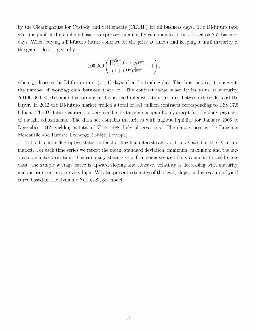
by the Clearinghouse for Custody and Settlements (CETIP) for all business days. The DI-futuro rate,
which is published on a daily basis, is expressed in annually compounded terms, based on 252 business
days. When buying a DI-futuro future contract for the price at time t and keeping it until maturity τ ,
the gain or loss is given by:
100.000
(∏ζ(t,τ)i=1 (1 + yi)
1252
(1 + ID∗)ζ(t,τ)252
− 1
),
where yi denotes the DI-futuro rate, (i − 1) days after the trading day. The function ζ(t, τ) represents
the number of working days between t and τ . The contract value is set by its value at maturity,
R$100, 000.00, discounted according to the accrued interest rate negotiated between the seller and the
buyer. In 2012 the DI-futuro market traded a total of 341 million contracts corresponding to US$ 17.5
billion. The DI-futuro contract is very similar to the zero-coupon bond, except for the daily payment
of margin adjustments. The data set contains maturities with highest liquidity for January 2006 to
December 2012, yielding a total of T = 1488 daily observations. The data source is the Brazilian
Mercantile and Futures Exchange (BM&FBovespa)
Table 1 reports descriptive statistics for the Brazilian interest rate yield curve based on the DI-futuro
market. For each time series we report the mean, standard deviation, minimum, maximum and the lag-
1 sample autocorrelation. The summary statistics confirm some stylized facts common to yield curve
data: the sample average curve is upward sloping and concave, volatility is decreasing with maturity,
and autocorrelations are very high. We also present estimates of the level, slope, and curvature of yield
curve based on the dynamic Nelson-Siegel model.
17
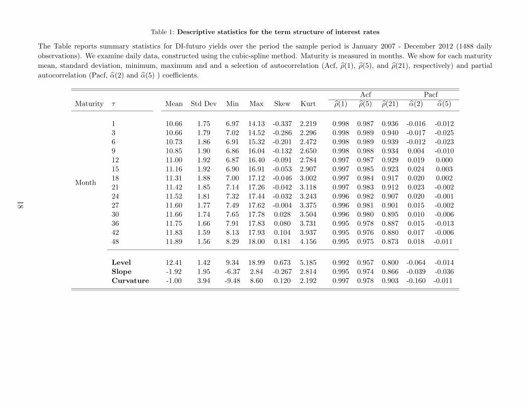
Table 1: Descriptive statistics for the term structure of interest rates
The Table reports summary statistics for DI-futuro yields over the period the sample period is January 2007 - December 2012 (1488 daily
observations). We examine daily data, constructed using the cubic-spline method. Maturity is measured in months. We show for each maturity
mean, standard deviation, minimum, maximum and and a selection of autocorrelation (Acf, ρ(1), ρ(5), and ρ(21), respectively) and partial
autocorrelation (Pacf, α(2) and α(5) ) coefficients.
Acf PacfMaturity τ Mean Std Dev Min Max Skew Kurt ρ(1) ρ(5) ρ(21) α(2) α(5)
Month
1 10.66 1.75 6.97 14.13 -0.337 2.219 0.998 0.987 0.936 -0.016 -0.0123 10.66 1.79 7.02 14.52 -0.286 2.296 0.998 0.989 0.940 -0.017 -0.0256 10.73 1.86 6.91 15.32 -0.201 2.472 0.998 0.989 0.939 -0.012 -0.0239 10.85 1.90 6.86 16.04 -0.132 2.650 0.998 0.988 0.934 0.004 -0.01012 11.00 1.92 6.87 16.40 -0.091 2.784 0.997 0.987 0.929 0.019 0.00015 11.16 1.92 6.90 16.91 -0.053 2.907 0.997 0.985 0.923 0.024 0.00318 11.31 1.88 7.00 17.12 -0.046 3.002 0.997 0.984 0.917 0.020 0.00221 11.42 1.85 7.14 17.26 -0.042 3.118 0.997 0.983 0.912 0.023 -0.00224 11.52 1.81 7.32 17.44 -0.032 3.243 0.996 0.982 0.907 0.020 -0.00127 11.60 1.77 7.49 17.62 -0.004 3.375 0.996 0.981 0.901 0.015 -0.00230 11.66 1.74 7.65 17.78 0.028 3.504 0.996 0.980 0.895 0.010 -0.00636 11.75 1.66 7.91 17.83 0.080 3.731 0.995 0.978 0.887 0.015 -0.01342 11.83 1.59 8.13 17.93 0.104 3.937 0.995 0.976 0.880 0.017 -0.00648 11.89 1.56 8.29 18.00 0.181 4.156 0.995 0.975 0.873 0.018 -0.011
Level 12.41 1.42 9.34 18.99 0.673 5.185 0.992 0.957 0.800 -0.064 -0.014Slope -1.92 1.95 -6.37 2.84 -0.267 2.814 0.995 0.974 0.866 -0.039 -0.036Curvature -1.00 3.94 -9.48 8.60 0.120 2.192 0.997 0.978 0.903 -0.160 -0.011
18

Figure 1 displays a three-dimensional plot of the data set and illustrates how yield levels and spreads
vary substantially throughout the sample. The plot also suggests the presence of an underlying factor
structure. Although the yield series vary heavily over time for each of the maturities, a strong common
pattern in the 14 series is apparent. For most months, the yield curve is an upward sloping function of
time to maturity. For example, last year of the sample is characterized by rising interest rates, especially
for the shorter maturities, which respond faster to the contractionary monetary policy implemented by
the Brazilian Central Bank in the first half of 2010. It is clear from Figure 1 that not only the level
of the term structure fluctuates over time but also its slope and curvature. The curve takes on various
forms ranging from nearly flat to (inverted) S-type shapes.
Figure 1: Evolution of the yield curve
Note: The figure plots the evolution of term structure of interest rates (based on DI-futuro contracts)for the time horizon of 2006:01-2012:12. The sample consisted of the daily yields for the maturitiesof 1, 3, 4, 6, 9, 12, 15, 18, 24, 27, 30, 36, 42 and 48 months.
4.1.1. Implementation details
The forecasting exercise is performed in pseudo real time, i.e. we never use information which is not
available at the time the forecast is made. For computing our results we use a rolling estimation window
of 500 daily observations (2 years). We have also estimated the models using an expanding window.
However, the RMSE results obtained were qualitatively similar to those presented here. These results
are available upon request. We produce forecasts for 1-week, 1-month, 2-month, and 3-month ahead.
The choice of a rolling scheme is suggested by two reasons. First, it is a natural way to avoid problems
of instability, see e.g. Pesaran et al. (2011). Second, having fixed the number of observations used to
compute the forecasts and therefore the resulting time series of the forecast errors allows the use of the
19

Giacomini & White (2006) test for comparing forecast accuracy. Such a test is valid provided that the
size of the estimation window is fixed.
We use iterated forecasts instead of direct forecasts for the multi-period ahead predictions. Marcellino
et al. (2006) compare empirical iterated and direct forecasts from linear univariate and bivariate models
by applying simulated out-of-sample methods and conclude that iterated forecasts typically outperform
the direct forecasts, and that the relative performance of the iterated forecasts improves with the forecast
horizon.
4.2. Results
4.2.1. Statistical evaluation
Table 2 reports statistical measures of the out-of-sample forecasting performance of ten alternative
individual models and five combination schemes for four forecast horizons. The first line in each panel
of the table reports the value of TRMSFE and RMSFE (expressed in basis points) for the random walk
model (RW), while all other lines reports statistics relative to the RW. Bold values indicate the model
with best performance in each maturity. In order to asses the statistical significance of these differences
in forecast, we use the test of conditional predictive ability proposed by Giacomini & White (2006).
20

Table 2: Relative (Trace)-Root Mean Squared Forecast Errors
The table reports relative root mean squared forecast errors (RMSFE) and trace RMSFE (TRMSFE) relative to the random walk model obtained by usingindividual yield models and different forecast combination methods, for the 1-day, 1-week, 1-month, 2-month, and 3-month forecast horizons. The evaluationsample is 2009:1 to 2012:12 (988 out-of-sample forecasts). The first line in each panel of the table reports the value of RMSFE and TRMSFE (expressed in basispoints) for the random walk model (RW), while all other lines reports statistics relative to the RW. The following model abbreviations are used in the table: AR(1)for the first-order univariate autoregressive model, VAR(1) for the first-order vector autoregressive model, BVAR refers to Bayesian VAR, DNS for the dynamicNelson-Siegel model, DSV for the dynamic Svensson model. CP refers to Cochrane & Piazzezi model, FB for the Fama-Bliss model, SR for slope regression,and CIR refers to Cox-Ingersol-Ross three factor model. FC-EW, FC-OLS and FC-RANK stand for forecast combinations based on equal weights, OLS-basedweights, and rank-weighted combinations, respectively. FC-RMSE and FC-MRMSE refer to forecast combinations base on the thick modeling approach withRMSE-weights and MSE-Frequency weights, respectively. Numbers smaller than one indicate that models outperform the RW, whereas numbers larger than oneindicate underperformance. Numbers in bold indicate outperformance in the maturity. Stars indicate the level at which the Giacomini and White (2006) testrejects the null of equal forecasting accuracy (∗, and ∗∗ mean respectively rejection at 10%, and 5% level).
Models TRMSFE
1- 3- 6- 9- 12- 15- 18- 21- 24- 27- 30- 36- 42- 48-
Month Month Month Month Month Month Month Month Month Month Month Month Month Month
PANEL A: Horizon = 1-day ahead
RW 0.074 0.038 0.040 0.052 0.060 0.066 0.071 0.076 0.079 0.081 0.084 0.086 0.088 0.091 0.094
AR(1) 1.002 0.992 0.994 0.998 1.000 1.001 1.001 1.002∗ 1.002∗ 1.003∗ 1.003 1.003 1.003 1.003 1.003
VAR(1) 1.043 0.905∗∗ 0.931∗∗ 0.993 1.020∗ 1.030∗ 1.046∗∗ 1.048∗∗ 1.056∗∗ 1.057∗∗ 1.054∗∗ 1.052∗∗ 1.052∗∗ 1.054∗∗ 1.051∗∗
BVAR 0.999 0.907∗∗ 0.927∗∗ 0.973∗∗ 0.990 0.998 1.002 1.004 1.005 1.004 1.004 1.004 1.005 1.005 1.005
DNS 1.638 2.633∗∗ 0.917∗∗ 1.978∗∗ 2.046∗∗ 1.841∗∗ 1.569∗∗ 1.112∗∗ 1.021∗∗ 1.065∗∗ 1.082∗∗ 1.056∗∗ 1.021 1.016 1.102∗∗
DSV 1.196 2.266∗∗ 0.913∗∗ 1.234∗∗ 1.033∗∗ 1.076∗∗ 1.086∗∗ 1.056∗∗ 1.031∗∗ 1.056∗∗ 1.074∗∗ 1.043∗∗ 1.034∗ 1.007 1.067∗∗
CP 1.012 0.878∗∗ 0.904∗∗ 0.964∗∗ 0.994 1.001 1.012 1.017 1.024∗∗ 1.026∗∗ 1.022∗∗ 1.021∗∗ 1.020∗ 1.024∗∗ 1.017
FB 0.992 0.990 0.918 0.960 0.975 0.983 0.988 0.992 0.995 0.997 0.997 0.997 0.997 0.999 1.000
SR 0.991 0.990 0.918 0.961 0.976 0.983 0.988 0.991 0.993 0.995 0.996 0.997 0.998 0.998 0.998
CIR 1.410 0.997 0.997 0.999 1.001 1.002 0.999 1.550 1.371 1.272 1.596 1.741 1.821 1.495 1.196
FC-EW 1.003 1.142∗∗ 0.923∗∗ 1.001∗∗ 1.021∗∗ 1.012 1.002 1.012∗∗ 0.998 0.996 0.997 0.995 0.997 0.997 1.006
FC-OLS 0.990 0.884∗∗ 0.911∗∗ 0.961∗∗ 0.976∗∗ 0.985∗∗ 0.988∗∗ 0.994∗∗ 0.994∗∗ 0.996∗∗ 0.997∗∗ 0.998∗∗ 0.998∗∗ 0.999∗∗ 0.999
FC-RANK 0.994 0.892∗∗ 0.905∗∗ 0.967∗∗ 0.983∗∗ 0.993∗∗ 0.993∗∗ 0.998 0.999 0.999 1.002 1.000 0.999 1.001 1.001
FC-RMSE 0.991 0.891∗∗ 0.906∗∗ 0.963∗∗ 0.978∗∗ 0.986∗∗ 0.990∗∗ 0.994∗∗ 0.996∗∗ 0.997∗∗ 0.997∗∗ 0.998∗∗ 0.998∗∗ 0.999 0.999
FC-MRMSE 0.991 0.890∗∗ 0.905∗∗ 0.964∗∗ 0.980∗∗ 0.987∗∗ 0.991∗∗ 0.994∗∗ 0.996∗∗ 0.997∗∗ 0.998∗∗ 0.998∗∗ 0.999 0.999 0.999
Continued on next page
21

Table 2 – Continued from previous page
Models TRMSFE
1- 3- 6- 9- 12- 15- 18- 21- 24- 27- 30- 36- 42- 48-
Month Month Month Month Month Month Month Month Month Month Month Month Month Month
PANEL B: Horizon = 1-week ahead
RW 0.171 0.121 0.120 0.141 0.154 0.164 0.174 0.181 0.183 0.184 0.187 0.188 0.188 0.189 0.192
AR(1) 1.009 0.985∗∗ 0.986 0.994 0.999 1.003 1.006 1.008 1.011 1.013 1.013 1.014 1.016 1.018∗ 1.019∗
VAR(1) 1.105 0.725∗∗ 0.764∗∗ 0.928 1.015 1.062 1.105∗∗ 1.130∗∗ 1.152∗∗ 1.162∗∗ 1.159∗∗ 1.160∗∗ 1.162∗∗ 1.169∗∗ 1.166∗∗
BVAR 0.995 0.757∗∗ 0.784∗∗ 0.907∗∗ 0.964 0.994 1.011 1.022 1.024 1.022 1.022 1.023 1.023 1.023 1.025∗
DNS 1.082 1.730∗∗ 0.754∗∗ 1.291∗∗ 1.340∗∗ 1.174∗∗ 1.029 0.988∗ 1.003 1.012 1.008 1.001 0.999 1.003 1.009
DSV 0.985 1.362∗∗ 0.742∗∗ 0.906∗∗ 0.908∗∗ 0.934∗∗ 0.962 0.972 0.980 0.991 0.991 0.977 0.988 1.003 1.022
CP 0.972 0.889∗∗ 0.902∗∗ 0.946∗∗ 0.961∗∗ 0.968∗∗ 0.977∗∗ 0.979∗∗ 0.982∗∗ 0.979∗∗ 0.979∗∗ 0.98∗∗ 0.980∗∗ 0.984∗∗ 0.984∗
FB 0.989 0.993 0.922 0.954 0.971 0.979 0.985 0.991 0.995 0.996 0.997 0.997 0.997 0.998 0.998
SR 0.990 0.994 0.924 0.956 0.973 0.981 0.987 0.991 0.994 0.996 0.997 0.998 0.999 1.001 1.000
CIR 1.420 1.942 2.281 2.043 2.213 1.935 1.503 1.149 1.136 1.012 1.048 1.060 1.084 1.029 1.106
FC-EW 0.972 0.738∗∗ 0.805∗∗ 0.957∗∗ 0.992∗∗ 0.996 0.993 0.988 0.987∗ 0.979 0.976∗∗ 0.978∗∗ 0.984∗∗ 0.989∗∗ 0.999
FC-OLS 0.957 0.752∗∗ 0.745∗∗ 0.892∗∗ 0.907∗∗ 0.931∗∗ 0.981∗∗ 0.983∗∗ 0.985∗∗ 0.983∗ 0.983∗∗ 0.984∗∗ 0.984∗∗ 0.986∗∗ 0.987
FC-RANK 0.969 0.748∗∗ 0.747∗∗ 0.886∗∗ 0.919∗∗ 0.937∗∗ 0.99∗∗ 0.993∗ 0.995 0.996 0.997 0.999 1.001 1.005 1.007
FC-RMSE 0.961 0.739∗∗ 0.746∗∗ 0.879∗∗ 0.912∗∗ 0.933∗∗ 0.984∗∗ 0.987∗∗ 0.988∗∗ 0.988∗ 0.988∗ 0.990 0.991 0.995 0.996
FC-MRMSE 0.960 0.739∗∗ 0.746∗∗ 0.879∗∗ 0.909∗∗ 0.933∗∗ 0.982∗∗ 0.986∗∗ 0.988∗∗ 0.986∗ 0.987∗ 0.988∗ 0.99 0.995 0.994
PANEL C: Horizon = 1-month ahead
RW 0.439 0.405 0.409 0.430 0.442 0.445 0.455 0.459 0.458 0.453 0.453 0.452 0.437 0.420 0.417
AR(1) 1.022 0.995 0.994 0.997 1.001 1.006 1.012 1.017 1.023 1.029 1.031 1.036 1.045∗ 1.056∗∗ 1.061∗∗
VAR(1) 1.038 0.451∗∗ 0.573∗∗ 0.749∗ 0.858 0.963 1.040∗ 1.101∗∗ 1.139∗∗ 1.162∗∗ 1.158∗∗ 1.159∗∗ 1.198∗∗ 1.230∗∗ 1.230∗∗
BVAR 0.954 0.585∗∗ 0.665∗∗ 0.818 0.911 0.963 0.995 1.019∗∗ 1.024∗∗ 1.020∗∗ 1.019∗ 1.019∗ 1.017 1.024 1.034∗
DNS 0.894 0.604∗∗ 0.580∗∗ 0.735∗∗ 0.804∗∗ 0.850∗∗ 0.894∗∗ 0.939∗ 0.970 0.979 0.973 0.972 0.991 0.998 0.980∗∗
DSV 0.850 0.536∗∗ 0.561∗∗ 0.683∗∗ 0.746∗∗ 0.803∗∗ 0.848∗∗ 0.882∗∗ 0.905∗∗ 0.923∗∗ 0.923∗∗ 0.919∗∗ 0.954∗∗ 0.981∗∗ 0.989∗
CP 0.976 0.958∗∗ 0.962∗∗ 0.970∗∗ 0.972∗∗ 0.976∗∗ 0.978∗∗ 0.978∗∗ 0.979∗∗ 0.978∗ 0.978∗ 0.977∗ 0.979∗∗ 0.983∗ 0.981
FB 0.992 0.996 0.970 0.978 0.983 0.986 0.990 0.994 0.996 0.997 0.997 0.998 0.998 0.998 0.998
SR 0.993 0.998 0.971 0.979 0.985 0.989 0.992 0.994 0.996 0.997 0.998 0.999 1.000 0.999 1.002
CIR 1.059 0.486 0.940 1.293 1.358 1.295 1.168 1.063 1.001 0.965 0.943 0.944 0.975 0.987 1.044
FC-EW 0.909 0.677∗∗ 0.743∗∗ 0.83∗∗ 0.878∗∗ 0.909∗∗ 0.93∗∗ 0.943∗∗ 0.948∗∗ 0.946∗∗ 0.944∗∗ 0.947∗∗ 0.960∗∗ 0.969∗ 0.976∗
FC-OLS 0.879 0.481∗∗ 0.563∗∗ 0.771∗∗ 0.763∗∗ 0.809∗∗ 0.856∗∗ 0.894∗∗ 0.927∗∗ 0.979∗∗ 0.981 0.973 0.993 1.007 1.015
FC-RANK 0.892 0.511∗∗ 0.565∗∗ 0.758∗∗ 0.771∗∗ 0.820∗∗ 0.929∗∗ 0.942∗∗ 0.949∗∗ 0.981∗∗ 0.968 0.970∗∗ 0.999∗∗ 1.014 1.021
FC-RMSE 0.870 0.497∗∗ 0.564∗∗ 0.711∗∗ 0.767∗∗ 0.817∗∗ 0.868∗∗ 0.892∗∗ 0.905∗∗ 0.978∗∗ 0.953 0.954 0.988 0.998 1.001
FC-MRMSE 0.871 0.494∗∗ 0.565∗∗ 0.716∗∗ 0.763∗∗ 0.816∗∗ 0.863∗∗ 0.886∗∗ 0.908∗∗ 0.979∗∗ 0.958 0.959∗ 0.993∗ 1.003 1.006
Continued on next page
22
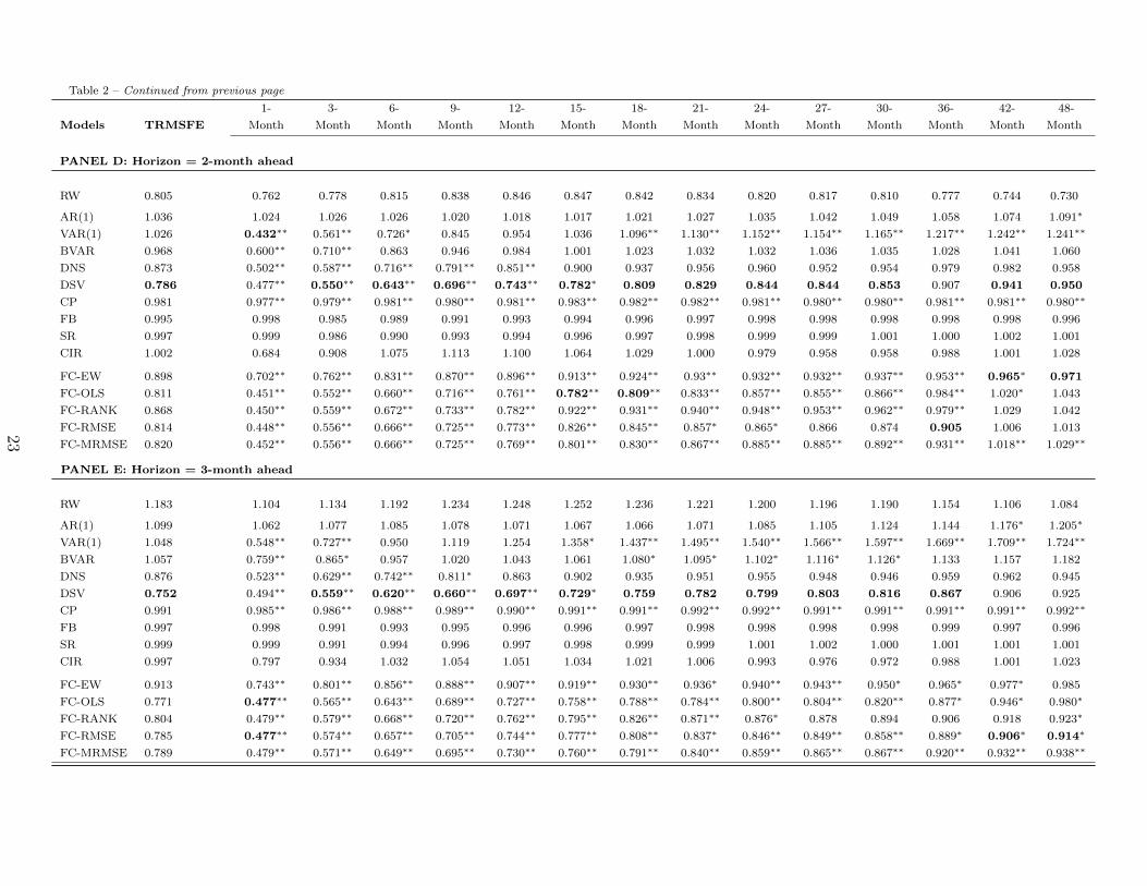
Table 2 – Continued from previous page
Models TRMSFE
1- 3- 6- 9- 12- 15- 18- 21- 24- 27- 30- 36- 42- 48-
Month Month Month Month Month Month Month Month Month Month Month Month Month Month
PANEL D: Horizon = 2-month ahead
RW 0.805 0.762 0.778 0.815 0.838 0.846 0.847 0.842 0.834 0.820 0.817 0.810 0.777 0.744 0.730
AR(1) 1.036 1.024 1.026 1.026 1.020 1.018 1.017 1.021 1.027 1.035 1.042 1.049 1.058 1.074 1.091∗
VAR(1) 1.026 0.432∗∗ 0.561∗∗ 0.726∗ 0.845 0.954 1.036 1.096∗∗ 1.130∗∗ 1.152∗∗ 1.154∗∗ 1.165∗∗ 1.217∗∗ 1.242∗∗ 1.241∗∗
BVAR 0.968 0.600∗∗ 0.710∗∗ 0.863 0.946 0.984 1.001 1.023 1.032 1.032 1.036 1.035 1.028 1.041 1.060
DNS 0.873 0.502∗∗ 0.587∗∗ 0.716∗∗ 0.791∗∗ 0.851∗∗ 0.900 0.937 0.956 0.960 0.952 0.954 0.979 0.982 0.958
DSV 0.786 0.477∗∗ 0.550∗∗ 0.643∗∗ 0.696∗∗ 0.743∗∗ 0.782∗ 0.809 0.829 0.844 0.844 0.853 0.907 0.941 0.950
CP 0.981 0.977∗∗ 0.979∗∗ 0.981∗∗ 0.980∗∗ 0.981∗∗ 0.983∗∗ 0.982∗∗ 0.982∗∗ 0.981∗∗ 0.980∗∗ 0.980∗∗ 0.981∗∗ 0.981∗∗ 0.980∗∗
FB 0.995 0.998 0.985 0.989 0.991 0.993 0.994 0.996 0.997 0.998 0.998 0.998 0.998 0.998 0.996
SR 0.997 0.999 0.986 0.990 0.993 0.994 0.996 0.997 0.998 0.999 0.999 1.001 1.000 1.002 1.001
CIR 1.002 0.684 0.908 1.075 1.113 1.100 1.064 1.029 1.000 0.979 0.958 0.958 0.988 1.001 1.028
FC-EW 0.898 0.702∗∗ 0.762∗∗ 0.831∗∗ 0.870∗∗ 0.896∗∗ 0.913∗∗ 0.924∗∗ 0.93∗∗ 0.932∗∗ 0.932∗∗ 0.937∗∗ 0.953∗∗ 0.965∗ 0.971
FC-OLS 0.811 0.451∗∗ 0.552∗∗ 0.660∗∗ 0.716∗∗ 0.761∗∗ 0.782∗∗ 0.809∗∗ 0.833∗∗ 0.857∗∗ 0.855∗∗ 0.866∗∗ 0.984∗∗ 1.020∗ 1.043
FC-RANK 0.868 0.450∗∗ 0.559∗∗ 0.672∗∗ 0.733∗∗ 0.782∗∗ 0.922∗∗ 0.931∗∗ 0.940∗∗ 0.948∗∗ 0.953∗∗ 0.962∗∗ 0.979∗∗ 1.029 1.042
FC-RMSE 0.814 0.448∗∗ 0.556∗∗ 0.666∗∗ 0.725∗∗ 0.773∗∗ 0.826∗∗ 0.845∗∗ 0.857∗ 0.865∗ 0.866 0.874 0.905 1.006 1.013
FC-MRMSE 0.820 0.452∗∗ 0.556∗∗ 0.666∗∗ 0.725∗∗ 0.769∗∗ 0.801∗∗ 0.830∗∗ 0.867∗∗ 0.885∗∗ 0.885∗∗ 0.892∗∗ 0.931∗∗ 1.018∗∗ 1.029∗∗
PANEL E: Horizon = 3-month ahead
RW 1.183 1.104 1.134 1.192 1.234 1.248 1.252 1.236 1.221 1.200 1.196 1.190 1.154 1.106 1.084
AR(1) 1.099 1.062 1.077 1.085 1.078 1.071 1.067 1.066 1.071 1.085 1.105 1.124 1.144 1.176∗ 1.205∗
VAR(1) 1.048 0.548∗∗ 0.727∗∗ 0.950 1.119 1.254 1.358∗ 1.437∗∗ 1.495∗∗ 1.540∗∗ 1.566∗∗ 1.597∗∗ 1.669∗∗ 1.709∗∗ 1.724∗∗
BVAR 1.057 0.759∗∗ 0.865∗ 0.957 1.020 1.043 1.061 1.080∗ 1.095∗ 1.102∗ 1.116∗ 1.126∗ 1.133 1.157 1.182
DNS 0.876 0.523∗∗ 0.629∗∗ 0.742∗∗ 0.811∗ 0.863 0.902 0.935 0.951 0.955 0.948 0.946 0.959 0.962 0.945
DSV 0.752 0.494∗∗ 0.559∗∗ 0.620∗∗ 0.660∗∗ 0.697∗∗ 0.729∗ 0.759 0.782 0.799 0.803 0.816 0.867 0.906 0.925
CP 0.991 0.985∗∗ 0.986∗∗ 0.988∗∗ 0.989∗∗ 0.990∗∗ 0.991∗∗ 0.991∗∗ 0.992∗∗ 0.992∗∗ 0.991∗∗ 0.991∗∗ 0.991∗∗ 0.991∗∗ 0.992∗∗
FB 0.997 0.998 0.991 0.993 0.995 0.996 0.996 0.997 0.998 0.998 0.998 0.998 0.999 0.997 0.996
SR 0.999 0.999 0.991 0.994 0.996 0.997 0.998 0.999 0.999 1.001 1.002 1.000 1.001 1.001 1.001
CIR 0.997 0.797 0.934 1.032 1.054 1.051 1.034 1.021 1.006 0.993 0.976 0.972 0.988 1.001 1.023
FC-EW 0.913 0.743∗∗ 0.801∗∗ 0.856∗∗ 0.888∗∗ 0.907∗∗ 0.919∗∗ 0.930∗∗ 0.936∗ 0.940∗∗ 0.943∗∗ 0.950∗ 0.965∗ 0.977∗ 0.985
FC-OLS 0.771 0.477∗∗ 0.565∗∗ 0.643∗∗ 0.689∗∗ 0.727∗∗ 0.758∗∗ 0.788∗∗ 0.784∗∗ 0.800∗∗ 0.804∗∗ 0.820∗∗ 0.877∗ 0.946∗ 0.980∗
FC-RANK 0.804 0.479∗∗ 0.579∗∗ 0.668∗∗ 0.720∗∗ 0.762∗∗ 0.795∗∗ 0.826∗∗ 0.871∗∗ 0.876∗ 0.878 0.894 0.906 0.918 0.923∗
FC-RMSE 0.785 0.477∗∗ 0.574∗∗ 0.657∗∗ 0.705∗∗ 0.744∗∗ 0.777∗∗ 0.808∗∗ 0.837∗ 0.846∗∗ 0.849∗∗ 0.858∗∗ 0.889∗ 0.906∗ 0.914∗
FC-MRMSE 0.789 0.479∗∗ 0.571∗∗ 0.649∗∗ 0.695∗∗ 0.730∗∗ 0.760∗∗ 0.791∗∗ 0.840∗∗ 0.859∗∗ 0.865∗∗ 0.867∗∗ 0.920∗∗ 0.932∗∗ 0.938∗∗
23

Panels (a) and (b) of Table 2 show results of 1-day-ahead and 1-week-ahead forecasts, respectively.
As documented in the literature, it is very difficult to outperform the RW for short horizons, since the
near unit root behavior of the yields seems to dominate and model-based information add little (Diebold
& Li, 2006; de Pooter et al. , 2010; Nyholm & Vidova-Koleva, 2012; Xiang & Zhu, 2013). Nevertheless,
we observe that some individual models and combination schemes are able to outperform the RW mainly
for short-term maturities. For instance, in the case of the 1-day-ahead forecasts we find that the FB and
SR specifications deliver lower TRMSFE in comparison to the RW. When looking at specific maturities,
we also find that some individual specifications outperformed the RW but only in the case of short
term maturities. Forecast combinations, on the other hand, also outperform the benchmark since they
achieve lower TRMSFE and lower RMSFE in the vast majority of the cases, for both short and long
term maturities. In the case of 1-week-ahead forecasts we observe that all forecast combination schemes
outperform the RW in terms of TRMSFE, and that the FC-OLS achieved the lowest TRMSFE among all
individual models and combination schemes. Moreover, forecast performance of both individual models
and combination schemes deteriorate as maturity grows longer.
The results for the 1-month-ahead forecasts are show in panel (c) of Table 2. We observe that for
short-term maturities several individual models and all combination schemes outperform the RW in
terms of lower RMSFE. The best overall performance is achieved by the DSV model, as it outperforms
the RW for all maturities. All forecast combinations considered also consistently outperform the RW as
they deliver lower TRMSFE and lower RMSFE in the vast majority of the cases.
Panel (d) of Table 2 reports the results for the 2-month-ahead forecasts. Even tough the DSV model
achieved the best overall performance in terms of TRMSFE, this model fails to outperform the RW
for maturities longer than 18 months. The same applies to the remaining individual models, with an
exception to the VAR and CP specifications. Forecast combination, in contrast, outperform the RW for
both short and long term rates. Similar results are observed in the panel (e) of Table 2 which reports
the results for the 3-month-ahead forecasts. In this case, forecast combination also seem to deliver a
more consistent outperformance in terms of lower RMSFE with respect to the RW across all maturities.
To explore the accuracy of the forecasts in different time intervals, we follow Welch & Goyal (2008)
and plot the difference in cumulative squared forecast errors between each of the the prediction models
and the RW along the out-of-sample evaluation period. Figures 2 and 3 display CSFE’s for the 1-week
and 3-month forecast horizons. The results for the remaining forecast horizons are similar and are
available upon request. Each line in the graph represents a different model and shows how a particular
24

model performs relative to the random walk benchmark. In particular, an increasing CSFE indicates
outperformance whereas a decreasing CSFE indicates underperformance with respect to the RW.
During the financial turmoil of the 2008-2009 period, interest rates initially went up and then declined
sharply from roughly 14% to a level of 8.5% for the short rate accompanied by a substantial widening
of spreads between long and short rates (see Figure 1). The CSFE graphs allow us to examine in detail
how different models perform during this period on a day-to-day basis. The CSFE graphs in panel (a)
of Figure 2 reveal that for the 1-week forecast horizons most individual models perform poorly with
respect to the RW, and that only the CP specification is able to maintain a weak outperformance even
in the crisis period. As for the forecast combinations, panel (b) of Figure 2 tells a different story. The
CSFE graphs indicate that the forecast combination schemes consistently outperform the RW in the
vast majority of the cases.
We also observe in the graphs that the outperformance of the combined forecasts is consistent and
stable throughout the entire out-of-sample period. This result suggest that the combination of forecasts
results in an improvement in forecast accuracy with respect to the benchmark model, and also with
respect to individual models. More specifically, it is often the case that the CSFE obtained with a
combination strategy for a given maturity and horizon is larger than the CSFEs obtained for single
models, highlighting the effects of model complementarities in producing precise forecasts.
Assessing the relative importance of individual models on the forecast combination schemes
A question so far unaddressed in the previous discussion is the relative importance of individual
models on the forecast combination schemes considered in the paper. In order to address this issue, we
report in Table 3 information regarding the average weights in each of the individual models across all
forecast combination schemes. The table report for each model the frequency of usage (i.e. the relative
number of times the model is selected) and the average weight (along with the 25% and 75% percentiles)
across all forecast combination schemes for the 1-week and 3-month forecast horizons and for the 3-, 12-,
30-, and 48-month rates. The results for the remaining forecast horizons and remaining maturity rates
are available upon requests.
25

Figure 2: Cumulative squared forecast errors (1-week forecast horizon)
Note: Figures (a) and (b) show the cumulative squared forecast errors (CSFE), relative to the random walk, of individualyield-only models in Panel (a) and of forecast combinations schemes in Panel (b). Figures shows CSFEs for a 3-month forecasthorizon. The evaluation sample is 2009:1 to 2012:12 (988 out-of-sample forecasts). Grey bars highlight recession periods.
(a) Individual models
(b) Forecast combinations
26

Figure 3: Cumulative squared forecast errors (3-month forecast horizon)
Note: Figures (a) and (b) show the cumulative squared forecast error (CSFE), relative to the random walk, of individualyield-only models in Panel (a) and of forecast combinations schemes in Panel (b). Figures shows CSFEs for a 3-month forecasthorizon. The evaluation sample is 2009:1 to 2012:12 (988 out-of-sample forecasts). Grey bars highlight recession periods.
(a) Individual models
(b) Forecast combinations
27
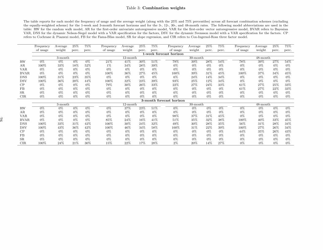
Table 3: Combination weights
The table reports for each model the frequency of usage and the average weight (along with the 25% and 75% percentiles) across all forecast combination schemes (excludingthe equally-weighted scheme) for the 1-week and 3-month forecast horizons and for the 3-, 12-, 30-, and 48-month rates. The following model abbreviations are used in thetable: RW for the random walk model, AR for the first-order univariate autoregressive model, VAR for the first-order vector autoregressive model, BVAR refers to BayesianVAR, DNS for the dynamic Nelson-Siegel model with a VAR specification for the factors, DSV for the dynamic Svensson model with a VAR specification for the factors. CPrefers to Cochrane & Piazzezi model, FB for the Fama-Bliss model, SR for slope regression, and CIR refers to Cox-Ingersol-Ross three factor model.
Frequency Average 25% 75% Frequency Average 25% 75% Frequency Average 25% 75% Frequency Average 25% 75%of usage weight perc. perc. of usage weight perc. perc. of usage weight perc. perc. of usage weight perc. perc.
1-week forecast horizon3-month 12-month 30-month 48-month
RW 0% 0% 0% 0% 21% 41% 30% 51% 79% 39% 28% 54% 78% 39% 27% 54%AR 100% 33% 18% 52% 1% 34% 28% 39% 0% 0% 0% 0% 0% 0% 0% 0%VAR 0% 0% 0% 0% 0% 0% 0% 0% 0% 0% 0% 0% 0% 0% 0% 0%BVAR 0% 0% 0% 0% 100% 36% 27% 45% 100% 39% 31% 45% 100% 37% 34% 45%DNS 100% 31% 23% 35% 0% 0% 0% 0% 6% 24% 14% 34% 0% 0% 0% 0%DSV 100% 36% 20% 44% 100% 32% 23% 39% 93% 25% 12% 34% 0% 0% 0% 0%CP 0% 0% 0% 0% 79% 30% 26% 33% 22% 27% 24% 33% 61% 27% 25% 33%FB 0% 0% 0% 0% 0% 0% 0% 0% 0% 0% 0% 0% 61% 27% 22% 33%SR 0% 0% 0% 0% 0% 0% 0% 0% 0% 0% 0% 0% 0% 0% 0% 0%CIR 0% 0% 0% 0% 0% 0% 0% 0% 0% 0% 0% 0% 0% 0% 0% 0%
3-month forecast horizon3-month 12-month 30-month 48-month
RW 0% 0% 0% 0% 0% 37% 23% 51% 0% 0% 0% 0% 0% 0% 0% 0%AR 0% 0% 0% 0% 0% 0% 0% 0% 0% 0% 0% 0% 0% 0% 0% 0%VAR 0% 0% 0% 0% 0% 0% 0% 0% 98% 37% 31% 45% 0% 0% 0% 0%BVAR 0% 0% 0% 0% 85% 24% 16% 41% 51% 35% 32% 38% 100% 40% 33% 45%DNS 100% 33% 31% 42% 100% 30% 24% 32% 49% 30% 28% 35% 56% 31% 28% 34%DSV 100% 43% 36% 42% 100% 46% 34% 58% 100% 31% 22% 39% 100% 27% 26% 34%CP 0% 0% 0% 0% 0% 0% 0% 0% 0% 0% 0% 0% 44% 35% 26% 43%FB 0% 0% 0% 0% 0% 0% 0% 0% 0% 0% 0% 0% 0% 0% 0% 0%SR 0% 0% 0% 0% 0% 0% 0% 0% 0% 0% 0% 0% 0% 0% 0% 0%CIR 100% 24% 21% 30% 15% 22% 17% 28% 2% 20% 14% 27% 0% 0% 0% 0%
28

Table 3 reveals that the allocation in individual models changes substantially across forecast horizons
and maturity rates. For instance, in the case of the 1-week forecast horizon, forecast combination for
the 3-month rate tend to select the AR, DNS and DSV specifications whereas for the 48-month rate
the mostly selected specifications are the RW, BVAR, CP and FB. As for the 3-month forecast horizon,
forecast combinations select mostly the DNS, DSV and CIR specifications, whereas for the 48-month
rate the selected specifications are BVAR, DNS, DSV, and CP.
4.2.2. Economic value of forecasts
In the previous subsection, we showed that alternative individual prediction models as well as fore-
cast combination schemes are able to deliver more accurate forecasts with respect to the benchmark
when considering statistical criteria. We observe, however, that in some instances the improvement in
forecasting performance (as indicated by lower forecasting errors) is small in magnitude. Therefore, a
question that remains unanswered is whether or not this statistical gain is also economically meaningful.
Table 4 reports the annualized Sharpe ratios of the mean-variance portfolios composed of Brazilian
DI-futuro contracts. We observe that in the vast majority of the instances, the mean-variance portfolios
obtained with individual models and with forecast combinations achieve statistically higher Sharpe ratios
in comparison to the mean-variance portfolios obtained with the random walk model. Moreover, this
result is robust to the value of the risk aversion coefficient and to the portfolio re-balancing frequency.
Small gains in forecasting performance can lead to Sharpe ratios that are substantially and statistically
higher than those obtained by the benchmark model. For instance, the 1-day ahead forecast errors of the
AR(1) model are not significantly better than the RW ones and, for some maturities, are significantly
worst. Nevertheless, all Sharpe ratios of daily rebalanced portfolios based on 1-day ahead forecasts from
AR(1) are larger than the Sharpe ratios of portfolios based on RW, and 3 out of 5 Sharpe ratios are
significantly larger. Additionally, the Sharpe ratio of the mean-variance portfolios obtained with the
RW specification with δ = 0.01 and daily re-balancing is 0.493 whereas the same figures for the BVAR
and FC-RMSE are, respectively, 1.021 and 1.483.
29

Table 4: Sharpe ratios of mean-variance portfolios
The Table reports annualized Sharpe ratios of the optimal mean-variance portfolios using DI-futuro contracts with maturities equal to 1, 3, 6, 9, 12, 15, 18, 21, 24, 27, 30, 36, 42and 48 months, where the risk-free rate used is the CDI, which is the Brazilian overnight rate. The following model abbreviations are used in the table: AR(1) for the first-orderunivariate autoregressive model, VAR(1) for the first-order vector autoregressive model, BVAR refers to Bayesian VAR, DNS for the dynamic Nelson-Siegel model, DSV forthe dynamic Svensson model. CP refers to Cochrane & Piazzezi model, FB for the Fama-Bliss model, SR for slope regression, and CIR refers to Cox-Ingersol-Ross three factormodel. FC-EW, FC-OLS and FC-RANK stand for forecast combinations based on equal weights, OLS-based weights, and rank-weighted combinations, respectively. FC-RMSEand FC-MRMSE refer to forecast combinations base on the thick modeling approach with RMSE-weights and MSE-Frequency weights, respectively. The optimal portfolios arere-balanced on a weekly, monthly, bimonthly, and quarterly basis. Asterisks indicate that the Sharpe ratio is statistically different with respect to that of the mean-varianceportfolio obtained with the random walk specification at a significance level of 10%.
Individual Models Forecast Combination
Model RW AR(1) VAR(1) BVAR DNS DSV CP FB SR CIR FC-EW FC-OLS FC-RANK FC-MSE FC-RMSEDaily re-balancing
Risk Aversion
δ = 0.01 0.493 0.542 0.693 1.021∗ 1.035∗ 0.691 0.430 0.445 0.649 0.217 0.779 0.676 0.641 1.185∗ 1.483∗
δ = 0.10 0.557 0.932∗ 0.595 0.912∗ 0.836 0.646 0.744 0.673 0.522 0.642 0.733 0.776 0.977∗ 1.230∗ 0.676δ = 0.50 0.657 1.079∗ 0.784 1.153∗ 0.555 0.547 0.252 0.257 0.277 0.576 0.829∗ 0.891∗ 0.773 0.842∗ 0.838∗
δ = 1.00 0.705 0.853 0.831 1.298∗ 0.757 0.671 0.545 0.559 0,459 0.568 0.823∗ 0.915∗ 0.800 0.840∗ 0.945∗
δ = 2.00 0.728 1.143∗ 1.013∗ 1.300∗ 0.867 0.801 0.582 0.582 0.512 0.607 0.893∗ 0.983∗ 0.863 0.912∗ 1.105∗
Weekly re-balancing
Risk Aversion
δ = 0.01 0.553 0.574 0.592 0.667 0.867∗ 0.898∗ 0.755 0.656 0.322 0.219 1.100∗ 1.164∗ 0.989∗ 1.115∗ 0.838∗
δ = 0.10 0.744 0.694 0.796 0.687 0.878 0.899 0.661 0.490 0.439 0.64 0.704 0.735 0.756 0.717 0.891∗
δ = 0.50 0.576 0.579 0.680 0.678 0.844∗ 0.802∗ 0.252 0.386 0.379 0.751 0.752 0.765 0.741 0.763 0.708δ = 1.00 0.618 0.694 0.830∗ 0.644 0.594 0.612 0.545 0.553 0.550 0.568 0.919∗ 0.999∗ 1.067∗ 0.939∗ 0.789δ = 2.00 0.620 0.635 0.605 0.890∗ 0.943∗ 0.787 0.582 0.498 0.582 0.678 0.939∗ 0.972∗ 0.950∗ 0.958∗ 1.050∗
Montly re-balancing
Risk Aversion
δ = 0.01 0.644 0.732 0.766 0.687 0.864∗ 0.872∗ 1.104∗ 0.783 0.573 0.254 0.829∗ 0.891∗ 0.773 0.842∗ 0.838δ = 0.10 0.658 0.750 0.718 0.667 0.881∗ 0.876∗ 0.714 0.508 0.521 0.790 0.710 0.802 0.636 0.702 0.893∗
δ = 0.50 0.634 0.741 0.690 0.678 0.995∗ 0.983∗ 0.470 0.447 0.444 0.725 0.969∗ 1.017∗ 1.018∗ 0.992∗ 1.009∗
δ = 1.00 0.788 0.860 0.820 0.850 1.049∗ 1.030∗ 0.507 0.528 0.526 0.555 0.937∗ 1.032∗ 0.912∗ 0.940∗ 0.687δ = 2.00 0.577 0.741 0.697 0.632 1.149∗ 1.199∗ 0.711 0.744 0.731 0.659 0.960∗ 1.028∗ 0.958∗ 0.970∗ 0.911∗
Bimontly re-balancing
Risk Aversion
δ = 0.01 0.533 0.535 0.521 0.702 0.795∗ 0.775∗ 0.645 0.967∗ 0.784 0.628∗ 0.823∗ 0.915∗ 0.800∗ 0.840∗ 0.945∗
δ = 0.10 0.543 0.543 0.521 0.702 0.805∗ 0.764∗ 0.726 0.593 0.595 0.985∗ 0.806 0.815∗ 0.758 0.793 0.931∗
δ = 0.50 0.562 0.554 0.521 0.718 0.865∗ 0.730 0.510 0.491 0.493 0.724 0.937∗ 1.032∗ 0.912∗ 0.940∗ 0.687δ = 1.00 0.762 0.756 0.736 0.600 0.817 0.717 0.485 0.444 0.467 0.506 0.956∗ 0.972∗ 0.988∗ 0.856 0.665δ = 2.00 0.551 0.554 0.618 0.625 0.794∗ 0.779∗ 0.767 0.706 0.704 0.793 0.948∗ 1.029∗ 0.886∗ 0.961∗ 0.831∗
Quartertly re-balancing
Risk Aversion
δ = 0.01 0.647 0.662 0.934∗ 0.670 0.815 0.727 0.956∗ 0.841 1.070∗ 0.760 0.893∗ 0.983∗ 0.863∗ 0.912∗ 1.105∗
δ = 0.10 0.686 0.667 0.843 0.670 0.815 0.727 0.766 0.702 0.714 0.948∗ 0.940∗ 0.952∗ 0.929∗ 0.932∗ 0.928∗
δ = 0.50 0.827 0.670 0.707 0.670 0.825 0.727 0.651 0.657 0.662 0.819 0.937 1.032∗ 0.912 0.940∗ 0.687∗
δ = 1.00 0.915 1.019 0.403 0.694 0.870 0.707 0,5 0.504 0.499 0.524 0.981 0.840 1.034 0.743 0.708δ = 2.00 0.694 0.598 0.688 0.672 0.883∗ 0.728 0.845 0.818 0.799 0.885 1.056∗ 1.146∗ 0.850 0.905∗ 0.848
30
We also observe that the forecast combinations deliver higher Sharpe ratios in comparison to those
obtained with individual models in most of the cases. For instance, the highest Sharpe ratio obtained
under daily re-balancing is achieved by the FC-RMSE (1.483), whereas for the weekly, bimonthly, and
quarterly re-balancing the highest Sharpe ratio is achieved by the FC-MSE (1.115), FC-OLS (1.032), FC-
OLS (1.146), respectively. These values are substantially higher than those obtained by the individual
models, including the benchmark specification. The only exception to this result is found in the the
monthly re-balancing frequency, since the highest Sharpe ratio is achieved by the DSV specification
(1.199).
One of the most important lessons from the economic evaluation of forecasts is that the differences
in performance in terms of Sharpe ratios are much more pronounced that those based on statistical
measures. In this sense, it seems to be much easier to distinguish between “good” and “bad” predictions
when looking at economic criteria. As we noted earlier, differences in statistical performance measures
are usually small in magnitude. In contrast, differences in Sharpe ratios tend to be much more evident.
In particular, we observe that in several cases the Sharpe ratios obtained by some forecast combination
schemes is twice as the ones obtained by some individual models.
4.2.3. Discussion
The results discussed in the previous Sections reveal that the statistical and economic evaluation of
forecast performance might be related, at least to some extent. We observe that those specifications that
deliver lower forecasting errors (measured in terms of RMSFE and TRMSFE) also tend to deliver mean-
variance portfolio with higher Sharpe ratios in comparison to the benchmark. However, how strong (or
weak) is this relation? In order to address this question, we plot in Figure 4 a two-dimensional graph
with the average value across all maturities of the RMSFE in the x-axis and the Sharpe ratios in the
y-axis for each forecast horizon. Moreover, we also report in the graph the value of the correlation
coefficient between both quantities.
Figure 4 indicates that the correlation coefficient between RMSFE and Sharpe ratios is negative
for all forecasting horizons. This result corroborates our previous findings and suggests that lower
forecasting errors is in fact associated to higher Sharpe ratios. In some instances, however, this relation
is weaker since the correlation coefficient between RMSFE and Sharpe ratios is closer to zero. For
example, the correlation coefficient for the 1-month-ahead is -0.43 whereas for the 3-month-ahead is
-0.09. This finding suggest that in some cases statistical and economic evaluation can provide different
answers about which candidate model is better. In fact, the results discussed in Tables 2 and 4 seem to
31

Figure 4: Relation between RMSFE and Sharpe ratios
Note: This figure presents scatter plots of out-of-sample economic performance measures againstRMSFE (root mean squared forecast error). The evaluation sample is 2009:1 to 2012:12 (988out-of-sample forecasts).
0.16 0.18 0.2 0.22 0.24 0.26
0.2
0.4
0.6
0.8
1
1.2
1.4
1.6Horizon = 1weak ahead ( ρ = − 0.24)
RMSE
Sha
rpe
Rat
io
δ = 0.01δ = 0.10δ = 0.50δ = 1.0δ = 2.0
0.36 0.37 0.38 0.39 0.4 0.41 0.42 0.43 0.44 0.45 0.460.2
0.4
0.6
0.8
1
1.2
1.4
1.6Horizon = 1month ahead ( ρ = − 0.43)
RMSE
Sha
rpe
Rat
io
δ = 0.01δ = 0.10δ = 0.50δ = 1.0δ = 2.0
0.65 0.7 0.75 0.8 0.85 0.90.2
0.3
0.4
0.5
0.6
0.7
0.8
0.9
1
1.1
1.2Horizon = 2month ahead ( ρ = − 0.26)
RMSE
Sha
rpe
Rat
io
δ = 0.01δ = 0.10δ = 0.50δ = 1.0δ = 2.0
0.8 0.9 1 1.1 1.2 1.3 1.4 1.5 1.6 1.70.2
0.3
0.4
0.5
0.6
0.7
0.8
0.9
1
1.1
1.2Horizon = 3month ahead ( ρ = − 0.09)
RMSE
Sha
rpe
Rat
io
δ = 0.01δ = 0.10δ = 0.50δ = 1.0δ = 2.0
32
corroborate this finding. We observe in these tables that the ranking of specifications based on statistical
performance can differ from the ranking based on an economic criterion. As we discussed previously, the
statistical evaluation in Table 2 and in the CSFE graphs in Figures 2 and 3 indicate that the forecast
combinations outperformed the remaining specification for shorter horizons, while for the longer horizons
some individual specifications such as the DSV model delivers more accurate forecasts. However, the
results for the economic evaluation in Table 2 reveal that forecast combinations tend to outperform
the remaining specification in the vast majority of the cases. In this sense, our evidence corroborate
the previous results in the literature, such as those reported in Leitch & Tanner (1991), Carriero et al.
(2012), and Cenesizoglu & Timmermann (2012).
5. Concluding remarks
This paper examines the statistical accuracy and economic value of modeling and forecasting the
term structure of interest rates using forecast combinations. Combined forecasts has been extensively
and successfully applied to forecast many economic time series (see, for example, Granger, 1989; Clemen,
1989; Granger & Jeon, 2004; Timmermann, 2006; Wallis, 2011). However, the literature on yield curve
forecasting has focused on performance evaluation of individual forecast models. Moreover, the majority
of yield curve studies considers only statistical evaluation of point forecasts, while the final goal of interest
rate forecasts is not to minimize mean squared prediction error but to improve financial decision making.
Thus, we conduct a detailed forecast performance evaluation of several univariate and multivariate
models based not only on statistical measures of accuracy, but also an economic evaluation using Sharpe
ratios of optimal mean-variance fixed income portfolios constructed based upon forecasts from individual
models and their alternative combinations. Differently from other yield curve studies, we use bootstrap
methods to determine if differences between Sharpe ratios are statistically different.
The results reveal that the statistical and economic evaluation of forecast performance might be
related. However, the correlations between RMSFE and Sharpe ratios are often very low and close to
zero in some cases. Moreover, the ranking of specifications based on statistical performance can differ
from the ranking based on economic criteria. More specifically, while the forecast combination schemes
outperformed in terms of RMSFE the remaining specification mostly for shorter forecast horizons, they
outperform individual models in the vast majority of cases when Sharpe ratio was considered.
33
References
Aiolfi, Marco, & Timmermann, Allan. 2006. Persistence in forecasting performance and condi-
tional combination strategies. Journal of Econometrics, 135(1-2), 31–53.
Ang, A., & Piazzesi, M. 2003. A no-arbitrage vector autoregression of term structure dynamics with
macroeconomic and latent variables. Journal of Monetary Economics, 50(4), 745–787.
Banbura, Marta, Giannone, Domenico, & Reichlin, Lucrezia. 2010. Large Bayesian vector
auto regressions. Journal of Applied Econometrics, 25(1), 71–92.
Bauwens, Luc, Lubrano, Michel, & Richard, Jean-Francois. 1999. Bayesian Inference in
Dynamic Econometric Models. Oxford University Press.
Caldeira, J. F., Moura, Guilherme V., & Portugal, Marcelo S. 2010. Efficient yield curve
estimation and forecasting in Brazil. Economia, 11(1), 27–51.
Caldeira, J. F., Moura, G. V., & Santos, A.A.P. 2012. Bond Portfolio Optimization: A Dynamic
Heteroskedastic Factor Model Approach. Working Paper, Department of Economics, Universidade
Federal de Santa Catarina.
Campbell, John Y, & Shiller, Robert J. 1991. Yield Spreads and Interest Rate Movements: A
Bird’s Eye View. Review of Economic Studies, 58(3), 495–514.
Carriero, Andrea, Kapetanios, George, & Marcellino, Massimiliano. 2012. Forecasting
government bond yields with large Bayesian vector autoregressions. Journal of Banking & Finance,
36(1), 2026–2047.
Cenesizoglu, Tolga, & Timmermann, Allan. 2012. Do return prediction models add economic
value? Journal of Banking & Finance, 36(11), 2974–2987.
Chen, Ren-Raw, & Scott, Louis. 1993. Maximum likelihood estimation for a multifactor equilibrim
model of the term structure of interest rates. The Journal of Fixed Income, 3(3), 14–32.
Chen, Ren-Raw, & Scott, Louis. 2003. Multi-Factor Cox-Ingersoll-Ross Models of the Term
Structure: Estimates and Tests from a Kalman Filter Model. The Journal of Real Estate Finance and
Economics, 27(2), 143–172.
34
Christoffersen, Peter F, & Diebold, Francis X. 1998. Cointegration and Long-Horizon Fore-
casting. Journal of Business & Economic Statistics, 16(4), 450–58.
Chyruk, Olena, Benzoni, Luca, & Ajello, Andrea. 2012. Core and ‘Crust’: Consumer Prices
and the Term Structure of Interest Rates. Tech. rept.
Clark, Todd E., & McCracken, Michael W. 2009. Improving Forecast Accuracy By Combining
Recursive And Rolling Forecasts. International Economic Review, 50(2), 363–395.
Clemen, Robert T. 1989. Combining forecasts: A review and annotated bibliography. International
Journal of Forecasting, 5(4), 559–583.
Cochrane, John H., & Piazzesi, Monika. 2005. Bond Risk Premia. American Economic Review,
95(1), 138–160.
Cox, J. C., Ingersoll, J. E., & Ross, S. A. 1985a. A theory of the term structure of interest rates.
Econometrica, 53(2), 385–407.
Cox, John C, Ingersoll, Jonathan E, Jr, & Ross, Stephen A. 1985b. An Intertemporal
General Equilibrium Model of Asset Prices. Econometrica, 53(2), 363–84.
Dai, Qiang, & Singleton, Kenneth J. 2000. Specification analysis of affine term structure models.
The Journal of Finance, 55(5), 1943–1978.
Dai, Qiang, Singleton, Kenneth J., & Yang, Wei. 2007. Regime shifts in a dynamic term
structure model of U.S. Treasury bond yields. Review of Financial Studies, 20(2), 1669–1706.
de Jong, Frank. 2000. Time series and cross-section information in affine term-structure models.
Journal of Business & Economic Statistics, 18(3), 300–314.
de Pooter, Michiel, Ravazzolo, Francesco, & van Dijk, Dick. 2010 (Mar.). Term structure
forecasting using macro factors and forecast combination. Working Paper 2010/01. Norges Bank.
Diebold, F., & Li, C. 2006. Forecasting the term structure of government bond yields. Journal of
Econometrics, 130(2), 337–364.
Diebold, F. X., Rudebusch, G. D., & Aruoba, S. B. 2006. The macroeconomy and the yield
curve: a dynamic latent factor approach. Journal of Econometrics, 131(1-2), 309–338.
35
Diebold, Francis X., & Rudebusch, Glen D. 2013. The Dynamic Nelson-Siegel Approach to
Yield Curve Modeling and Forecasting. Princeton University Press.
Doan, Thomas, Litterman, Robert B, & Sims, Christopher A. 1986. Forecasting and condi-
tional projection using realistic prior distribution. Tech. rept. Federal Reserve Bank of Minneapolis.
Duffee, G. R. 2002. Term premia and interest rate forecasts in affine models. Journal of Finance,
57(1), 405–443.
Duffie, Darrell, & Kan, Rui. 1996. A Yield-Factor Model Of Interest Rates. Mathematical Finance,
6(4), 379–406.
Fama, Eugene F., & Bliss, Robert R. 1987. The information in long-maturity forward rates. The
American Economic Review, 680–692.
Geweke, John, & Amisano, Gianni. 2011. Optimal prediction pools. Journal of Econometrics,
164(1), 130–141.
Giacomini, Raffaella, & White, Halbert. 2006. Tests of Conditional Predictive Ability. Econo-
metrica, 74(6), 1545–1578.
Granger, Clive W. J., & Jeon, Yongil. 2004. Thick modeling. Economic Modelling, 21(2),
323–343.
Granger, Clive W. J., & Pesaran, M. Hashem. 2000. Economic and statistical measures of
forecast accuracy. Journal of Forecasting, 19(7), 537–560.
Granger, Clive W.J. 1989. Combining Forecasts–Twenty Years Later. Journal of Forecasting, 8(3),
167–173.
Granger, Clive W.J., & Machina, Mark J. 2006. Forecasting and Decision Theory. Handbook
of Economic Forecasting, vol. 1. Elsevier. Chap. 2, pages 81–98.
Hendry, David F, & Clements, Michael P. 2004. Pooling of forecasts. The Econometrics Journal,
7(1), 1–31.
Hordahl, P., Tristani, O., & Vestin, D. 2006. A joint econometric model of macroeconomic and
term-structure dynamics. Journal of Econometrics, 131(1-2), 405–444.
36

Jagannathan, Ravi, & Ma, Tongshu. 2003. Risk reduction in large portfolios: Why imposing the
wrong constraints helps. The Journal of Finance, 58(4), 1651–1684.
Jungbacker, B., & Koopman, S.J. 2008. Likelihood-based analysis for dynamic factor models.
Tinbergen Institute Discussion Paper. found on http://www.tinbergen.nl.
Korn, Olaf, & Koziol, Christian. 2006. Bond portfolio optimization. The Journal of Fixed
Income, 15(4), 48–60.
Ledoit, O., & Wolf, M. 2008. Robust performance hypothesis testing with the Sharpe ratio. Journal
of Empirical Finance, 15(5), 850–859.
Leitch, Gordon, & Tanner, J Ernest. 1991. Economic forecast evaluation: profits versus the
conventional error measures. The American Economic Review, 81(3), 580–590.
Litterman, Robert B. 1986. Forecasting with Bayesian vector autoregressions: five years of experi-
ence. Journal of Business & Economic Statistics, 4(1), 25–38.
Marcellino, M., Stock, J., & Watson, M. 2006. A comparison of direct and iterated multistep
AR methods for forecasting macroeconomic time series. Journal of Econometrics, 135(1-2), 499–526.
Markowitz, H. 1952. Portfolio selection. Journal of Finance, 7(1), 77–91.
McCracken, M. W. 2007. Asymtoptics for out of sample tests of Granger Causality. Journal of
Econometrics, 140(2), 719–752.
McCracken, Michael W. 2000. Robust out-of-sample inference. Journal of Econometrics, 99(2),
195–223.
McCulloch, J. H. 1975. The tax-adjusted yield curve. Journal of Finance, 30(3), 811–30.
Morales-Arias, Leonardo, & Moura, Guilherme V. 2013. Adaptive forecasting of exchange
rates with panel data. International Journal of Forecasting, 29(3), 493 – 509.
Moench, Emmanuel. 2008. Forecasting the yield curve in a data-rich environment: a no-arbitrage
factor-augmented VAR approach. Journal of Econometrics, 146(1), 26–43.
Nelson, Charles R., & Siegel, Andrew F. 1987. Parsimonious modeling of yield curves. The
Journal of Business, 60(4), 473–489.
37

Newbold, P., & Harvey, I. H. 2002. Forecast combination and encompassing. In M. P. Clements,
and D. F. Hendry (Eds.), A companion to economic forecasting. Blackwell Publishers.
Nyholm, Ken, & Vidova-Koleva, Rositsa. 2012. Nelson-Siegel, Affine and Quadratic Yield Curve
Specifications: Which One is Better at Forecasting? Journal of Forecasting, 31(6), 540–564.
Pearson, Neil D, & Sun, Tong-Sheng. 1994. Exploiting the Conditional Density in Estimating the
Term Structure: An Application to the Cox, Ingersoll, and Ross Model. Journal of Finance, 49(4),
1279–1304.
Pesaran, M. Hashem, & Timmermann, Allan. 2007. Selection of estimation window in the
presence of breaks. Journal of Econometrics, 137(1), 134–161.
Pesaran, M. Hashem, Pick, Andreas, & Timmermann, Allan. 2011. Variable selection, estima-
tion and inference for multi-period forecasting problems. Journal of Econometrics, 164(1), 173–187.
Pesaran, M.H., & Skouras, S. 2002. Decision-based methods for forecast evaluation. A Companion
to Economic Forecasting, 241–267.
Piazzesi, Monika, & Schneider, Martin. 2009. Trend and cycle in bond premia. Tech. rept.
Svensson, Lars E. O. 1994 (Sept.). Estimating and interpreting forward interest rates: Sweden
1992-1994. IMF Working Papers 94/114. International Monetary Fund.
Timmermann, Allan. 2006. Forecast combinations. Handbook of economic forecasting, 1, 135–196.
Wallis, Kenneth F. 2011. Combining forecasts–forty years later. Applied Financial Economics,
21(1-2), 33–41.
Welch, Ivo, & Goyal, Amit. 2008. A Comprehensive Look at The Empirical Performance of Equity
Premium Prediction. Review of Financial Studies, 21(4), 1455–1508.
West, Kenneth D. 1996. Asymptotic Inference about Predictive Ability. Econometrica, 64(5), 1067–
84.
Xiang, Ju, & Zhu, Xiaoneng. 2013. A Regime-Switching Nelson-Siegel Term Structure Model and
Interest Rate Forecasts. Journal of Financial Econometrics, forthcoming.
38