Annals of Tropical Medicine and Parasitology, Vol. 90, No.3, 225-241 (1996)

REVIEW

Predicting the distribution of tsetseflies in West Africa using temporalFourier processed meteorologicalsatellite data

By D. J. ROGERS, S. I. KI\Y AND M. J. PACKERTrypanosomiasis and Land Use in Africa (TALA) Research Group, Departmentof Zoology, University of Oxford, South Parks Road, Oxford OX1 3PS, U.K.

Received and accepted 10 April 1996

An example is given of the application of remotely-sensed, satellite data to the problems of predicting thedistribution and abundance of tsetse flies in West Africa. The distributions of eight species of tsetse,Glossina morsitans, G. longipalpis, G. palpalis, G. tachinoides, G. pallicera, G. fusca, G. nigrofusca andG. medicorum in ate d'Ivoire and Burkina Faso, were analysed using discriminant analysis applied totemporal Fourier-processed surrogates for vegetation, temperature and rainfall derived from meteorologi-cal satellites. The vegetation and temperature surrogates were the normalized difference vegetation indexand channel-4-brightness temperature, respectively, from the advanced, ve~'-high-resolution radiometerson board the National Oceanic and Atmospheric Administration's polar-orbiting, meteorological satel-lites. For rainfall the surrogate was the Cold-Cloud-Duration (CCD) index derived from the geostation-ary, Meteosat satellite series. The presence or absence of tsetse was predicted with accuracies rangingfrom 670/0-1000/0 (mean=82'3%). A further data-set, for the abundance of five tsetse species across thenorthern part of ate d'lvoire (an area of about 140 000 km1, was analysed in the same way, andfly-abundance categories predicted with accuracies of 300/0-1000/0 (mean = 73'00/0). The thermal dataappeared to be the most useful of the predictor variables, followed by vegetation and rainfall indices.Refinements of the analytical technique and the problems of extending the predictions through space andtime are discussed.

The sensitivity to climate of arthropods ingeneral, and insect vectors in particular, hasalready been stressed in relation to the trans-mission of vector-borne disease transmission.Hay et al. (1996) explained how remote-sensing, satellite platforms can provide datathat are suitable surrogates for the traditionalmeteorological data that, in the past, have beencorrelated with both vector abundance andvector-mortality rates. They also explained thesteps in image processing that lead to a varietyof vegetation, thermal and rainfall indices, withemphasis on those platforms such as theNational Oceanic and Atmospheric Adminis-tration's (NOAA), polar-orbiting meteoro-

logical satellites and Meteosat satellites whichprovide frequent coverages from which rela-tively cloud-free views of the Earth's surface,or of cloud-top temperatures, can be produced.

Such multi-temporal data may be usedto give a realistic picture of average monthlyand annual values of vegetation and climateand have recently been used to describe thedistributions of several species of tsetse fly:Glossina morsitans Westwood in Zimbabwe(Rogers and Williams, 1993); G. morsitans andG. pallidipes Austen in Kenya and Tanzania(Rogers and Randolph, 1993); and G. palpalispalpalis (Robineau-Oesvoidy), G. tachinoidesWestwood, G. morsitans submorsitans

<rJ 1996 Liverpool School of Tropical Medicine0003-4983/96/030225+ 17512.00/0

226 ROGERS ET AL.

MATERIALS ,"-NO METHODS

Tsetse-fly DistributionsThe distributions of tsetse in Cote d'lvoire andBurkina F aso were taken from maps publishedby the Office de la Recherche Scientificet Technique d'Outre-Mer (ORSTOM)(Laveissiere and Challier, 1977, 1981). Thesemaps are compendia of information gatheredover the preceding decades and record species'presence at a spatial resolution of 0.167°. Theoriginal data sources do not give completespatial coverage, and the maps do not neces-sarily record fly presence in areas where aspecies was thought to be ubiquitous by thecompiling authors (e.g. G. palpalis in thesouthern part of COte d'lvoire). Thus, whilstrecords of fly presence on these maps arehistorically accurate, records of absence areoccasionally misleading. The distributionsof eight species of tsetse were used in thepresent analysis: G. morsitans submorsitans;G. longipalpis; G. palpalis s.l.; G. tac/rinoides;G. pa/licera Bigot; G. fusca; G. nigrofuscaNewstead; and G. medico rum Austen.

Newstead, G. longipalpis Wiedemann andG. Jitsca Walker in Togo (Rogers e1 al., 1994).These studies extended previous research inwhich tsetse-fly mortality rates (Rogers andRandolph, 1986, 1991), distribution (Gaschen,1945), abundance (Fairbairn and Culwick,1950) and infection rates (Ford and Leggate,1961) and prevalence of human sleeping sick-ness (Rogers and Williams, 1993) were relatedto ground-based measures of climate basedon synoptic or contemporary meteorologicalrecords.

The problems of processing large amountsof satellire data have led to the developmentof a variety of data-reduction methods. Inthe case of multi-temporal data, principal-components analysis of monthly, normalizeddifference vegetation indices (NDVI), derivedfrom the advanced, very-high-resolution radi-ometers (A VRRR) on board the NOAA seriesof satellites, usually gives a first componentobviously correlated with the mean vegetationindex f(H" the year. The second and thirdcomponents are related to seasonality, which isespecially pronounced in the savannah regionsof Afria (Townshend and Justice, 1986;Eastman and Fulk, 1993). An alternativeapproach to data reduction, using temporalFourier processing, gives results that haverecently been related to regional- andcontinenral-scale, biological processes (.'\ndrese1 al., 1994; Olsson and Eklundh, 1994; Rogersand "'.illiams, 1994; Verhoef e1 al., 1996).When Fourier analysis was applied to monthlyNDVl <bta for Africa, it was found that theannual, bi-annual and tri-annual cycles (called'compo~ts' in the analysis) explained a largepart of the variability of the annual NDVIsignal. Features of the Fourier analysis of thewhole-.\frica ~D'vl were related both to eco-logical IJanerns, such as the savannah regionsof Afria or the Gezira irrigation scheme insouthern Sudan, and to ecological processes,such as the seasonal groWth of vegetation alongthe River ~ile (Rogers and Williams, 1994).The present review describes the application ofthese techniques to the description of thedistribution and abundance of eight species oftsetse in Cote d'Ivoire and Burkina Faso, WestAfrica.

~I

Tsetse-fly AbundanceThe abundance of flies in the northern part ofCOte d'!voire was monitored by a joint Foodand Agriculture Organization/German Tech-nical Assistance (F AO/GTZ) project that ranfrom 1979 to 1980 and produced detailed mapsof fly distributions at scales of I: I 000 000 and1:200 000 (Anon., 1982). The data at a spatialresolution of 0.250. are used in the presentanalysis. Flies were sampled using Challier /Laveissiere traps (Challier and Laveissiere,1973) placed in suitable habitats by the surveyteams and left for short periods before collec-tion and removal. Given the very large areasampled and the short sampling time in eachhabitat, these data are likely to be affectedby a number of confounding effects such assampling errors, poor ".eather at the time ofsampling and seasonali~., so only the meanvalues (flies/trap per nominal 6-h trappingsession) were analysed.

Some of the species present in the regionwere inadequately sampled by the traps used inthe surveys, and supplementary catches using

SATELLITE DATA AND TSETSE-FLY DISTRIBUTIONS 227

hand nets were recorded separately on themaps. The coverage using this method wasrelatively poor, however, and these resultshave not been included in the present analysis,which is based entirely upon the trap catchesof G. morsitans, G. longipalpis, G. palpalis,G. tachinoides and G. fusca.

Cold-cloud-duration (CCD) imagery wasobtained from the F AO-ARTEMIS programas 5-year, monthly means for the period 1988-1992. The CCO imagery has been correlatedwith surface rainfall measurements as part ofthe Tropical Applications in Meteorolo~. ofSatellite and other data (T AMSA T) programwithin the area covered by the present tsetsesurveys (Snijders, 1991).

Oigital-elevation-model (OEM) data wereobtained from a O.O83°-resolution elevationsurface for Africa, produced by the GlobalLand Information System (GLIS) of theUnited States Geological Survey, EarthResources Observation Systems (USGS,EROS) data centre. The original files wereresampled to a 7.6 x 7.6 km resolution imageto ensure compatibilit). with the other data

layers.

Satellite-data Processing andData ReductionMulti-temporal satellite data produce multi-variate data-sets for each unit area (pixel)within an image. Each of the 12, monthlvMVC of each of the image types forms a singl~axis in a multi-variate space defining the en-vironment of the vector. Many of these axesare strongly correlated with each other be-cause, for example, a pixel with a high :t\TDVIin one month is likely to have a high NDVI inother months. This indicates that data reduc-tion (i.e. ordi~tion) could be achieved, with-out loss of information, by replacing the rawimagery with some combined signal derivedfrom these highly correlated values.

The simplest combination is obviously thearithmetic mean, and seasonal variability maybe captured b)' the variance or standard devi-ation of the mean. More complex ordinationtechniques generally involve projecting thedata onto a rotated (usually orthogonal) set ofaxes (called 'principal components') such thatthe first new axis captures the largest pro-portion of data variance, the second capturesthe largest proportion of the remaining vari-ance, and so on. Principal-components analysis(PCI\) retains the same number of axes as theoriginal data-set, but the sequential partition-ing of the variance often means that many of

Satellite DataNDVIs are derived from readings in channels1 and 2 (ChI and Chz, respectively) ofthe A \'HRR on board the NOAA series ofmeteorological satellites, being calculated as

(Chz -Chl)/(Chz+Chl).Prince et al. (1990) have described the ap-

plication of NDVI data to a range of biologicalproblems and Hay et al. (1996) not onlydescribed their application to arthropod vec-tors of disease specifically but also reviewedalternative vegetation indices. 1982-90 ten-day'dekadal' maximum-value-composite (M\TC)NDV1 data (Holben, 1986) were obtained fromthe Food and Agriculture Organization's(F AO) African Real Time EnvironmentalMonitoring using Meteorological Satellites(ARTEMIS) program at 7.6 x 7.6 km resol-ution. The registration of these images waschecked against a geo-referenced 'master'image, and corrections made where necessa~-.This involved shifting images by 0-3 pixelsin an east-west or north-south direction, de-pending on the scene. The raw imagery wasthen corrected for satellite-sensor drift inchannell using calibration coefficients derivedby Los (1993), and then maximum-value com-posited by selecting the highest value of thedekadal pixels for each site within each month,to produce a set of monthly images for further

analvsis.A \'HRR-channel-4-brightness temperature

correlates with air temperature at the Earth'ssurface (Hay et al., 1996). Dekadal dataat 7.6 x 7.6 km spatial resolution from thearchives of the Global Inventory Monitoringand Modelling Systems (GI~L\1S) group atthe NASA Goddard Space Flight Center weremaximum-value composited for the period1987-1992. Monthly image~- was later pro-duced, again by MVC, and used in the present

analysis.

228 ROGERS ET AL

where p= 1, ...[(NI2) -1]. The componentat a frequency wp=2nplN is called thepth harmonic and, for all P # N /2, theseharmonics may be written in the equivalentform

apcoswpt+ bpsin(J)pt= Rpcos«(J)pt+ <P,> 3)

where Rp is the amplitude of the pth harmonic

= "(lIp2 + bp2)

and <t>p is the phase of the pth harmonic(Chatfield, 1980)

-1,-bpi ap).

= tan

The effect of Fourier analysis is to partition thevariability of the time-series into (orthogonaland thus uncorrelated) components at frequen-cies of 21l/ N, 41l/ N, 61l/ N ..., 1l, or periodsequal to 1, 1/2, 1/3, ...2/ N times theduration of the observations, N. If monthlyobservations are taken, Fourier analysis canpartition the time-series into frequenciesequivalent to periods ranging from as long asthe whole time-series, down to 2 months(higher frequencies, i.e. shorter period cycles,cannot be distinguished by monthly data). FullFourier analysis exactly describes the originaldata set [since the Fourier series in eqn (1)contains N parameters to describe N obser-vations], but not all harmonics may be con-tributing equally to this description. Thefollowing relationship, known as Parseval'stheorem, applies to the Fourier representationof x,

the axes in principal-component space areeffectively redundant because they explainonly a very small proportion of the variance inthe original data-set (Green, 1978). Projectionof the original data-set onto the principalcomponent axes involves applying a series ofcoefficients or weights to the raw data, effec-tively to achieve the desired axis rotation (theweights are the cosines of the angles betweenthe original and rotated co-ordinate axes). Datavalues in the original co-ordinate system allcontribute (via their weighted values) to eachprincipal-component-axis score. Thus, for ex-ample, a series of 12, monthly images, fromJanuary-December, may be subjected to PCAand every month would then contribute toeach of the 12 resulting principal-componentaxes. If, however, only the firsr-few principal-component axes explain the great majority ofthe variance in the original data, only theseneed be used in further analysis. PCA is notindependent of the scale of the original axesand it is generally necessary to standardize (ortransform) the raw variables to roughly similarvariances before analysis, or else to use thecorrelation matrix in the analysis (Marriott,1974). This makes it difficult to extend theresults of PCA to other times and placesbecause principal-component-axis rotation isuniquely determined by the original set ofobservational data (the 'training set').

An entirely different approach to the sameproblem of data reduction was suggested bythe literature on time-series analysis (e.g.Chatfield, 1980). The time-series Xt may bedescribed by a Fourier series representationwhere

(4)N/2-1

I:(X,-i)2/N= L R;/2+a2NlZo0=1

(1)

N/2-1

%,=110+ L [lIpcos(27tpt/N)p=l

+b~in(27tpt/ N)] +1I,IV/2COS7tt

t=I,2, .lV, and the coefficients ap and bp aredefined as follows:

a =x0

aNn = I:(-I)tXt/N

(2)ap = 2[I:Xtcos(21tpt/ N)]/ N

bp = 2[I:x,sin(21tpt/ N)]/ N

This equation states that a quantity very simi-lar to the variance of the original observations[the left-hand side of the equation, but withthe divisor N rather than (N -1)] is the sumof the contributions of each of the harmonicsfor values of p from 1 to N /2, where Rj /2 isthe contribution of the pth harmonic.

The combination of the orthogonality of theharmonics in the Fourier-series representation

SATELLITE DATA A.'\JD TSETSE-FLY DISTRIBL'TIONS 229

of multi-temporal satellite data and the (per-haps illusory) biological transparency of theinterpretation of these harmonics makes thisapproach to data reduction especially attractiveto biologists (Rogers and Williams, 1994). Ineffect, it may be possible to reduce a monthlyor dekadal data stream covering 10 or moreyears to just seven variables (the mean of thewhole series and the amplitude and phases ofthe first three Fourier components) without asignificant loss of information.

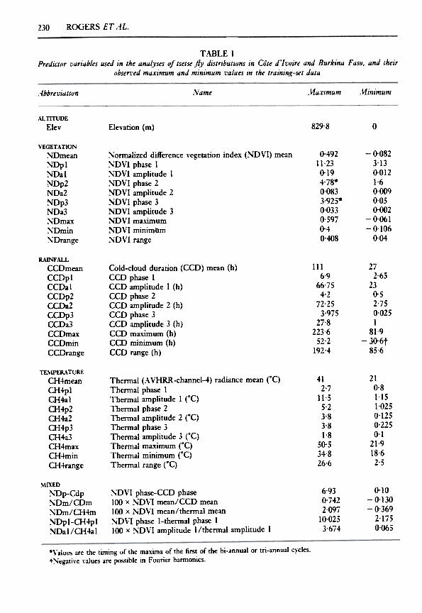
For the present study, each of the NDVI,channel-4-brightness-temperature and CCD,monthly-image data-sets were subjected totemporal Fourier processing and the means,amplitudes and phases of the annual, bi-annualand tri-annual cycles calculated. These vari-ables were stored as new image layers foranalysis, at the same spatial resolution as theoriginal imagef).. The combined (i.e. annualplus bi-annual plus tri-annual cycle) Fourierdescription of the original signal was alsocalculated (a summation that essentiallysmooths the original data-set) and its mini-mum, maximum and range were recorded foruse in the analysis. In addition, certain combi-nations of the Fourier-processed signals werecalculated, such as the ratio of ~~VI to meanvalues of channel-4-brightness temperatures,which has been shown to be a more stableindicator of vegetation type than either vari-able alone (Lambin and Ehrlich, 1995, 1996).A full list of predictor variables used in thisstudy is given in Table 1.

All satellite imagery was further processedby selecting a block of 2 x 2 pixels positionedat the centre of each grid square on thefly-distribution, and the mean values for eachsquare were used in further analyses.

I

,

(=dlsperslon) matnx (\..freen, l'JIO). lill t:qn(5), the subscript n for the number of variableshas been dropped for clarity.] Thus, theMahalanobis distance is the distance betweenthe sample centroids adjusted for their com-mon co-variance. In the case of the Euclideandistance, dtz, the co-variances are zero, so thatthe co-variance matrix C~ equals c~ -I or I,

the identity matrix (with values of I along thediagonal and 0 elsewhere). This reducesthe equation for Dtz to that for dtz' If the

Data AnalysisThe reduced-dimension data-set produced bythe methods outlined above form the set ofpredictor variables for describing the species'distributions and abundance. Of the methodsavailable, such as correspondence analysis (TerBraak, 1986; Hill, 1991), projection pursuit,nearest neighbour and neural network analysis(Williams et ai., 1992), this review concentrateson the use of various forms and modifications

~

of discriminant analvsis; these are relativelveasy to apply and provide biological insightinto the nature of the limits to the distributionand abundance of vector species. The simpleproblem of describing the distribution of avector is taken to illustrate the techniques.

In its simplest form, discriminant analysisassumes a multi-variate normal distribution ofthe predictor variables and a common within-group co-variance of the variables for all pointsdefining vector presence and vector absence.The mean values of the predictor variables insites of vector presence and absence, and thewithin-group co-variance matrix, are estimatedfrom representative samples from reliable dis-tribution maps (the 'training sets'). Means ofmulti-variate distributions are referred to ascentroids and are defined by mathematical vec-tors (~) where n is the number of dimensions(i.e. variables). The Mahalanobis distance, d,is the distance between two multi-variate dis-tribution centroids, or between a sample pointand a centroid, and is a generalization of thetraditional squared Euclidean distance, ~:

dt2 = (X";- -i;)'(X";- -i;) =d'd

and

Dt2 = (X";- -i;)'C-;' 1 (X";- -i;) =d'C-;' Id (5)

where dfl and Dfl are, respectively, theEuclidean and Mahalanobis distances betweengroup I (e.g. for vector absence) and group 2.(e.g. for vector presence), d is (XI -Xl)' witlJthe subscripts again referring to the tw(]groups (or, alternatively, 1 and 2 might referto a point and a centroid), and Cw -I is the

inverse of the within-groups co-varianct..'~"""" rT- ---

ROGERS ET AL.230

T.WLE IPredictor vllrillbles used in the IInlllyses of tsetse fly distributions in Cote d'/voire IInd Burk1nll FIISO, IInd their

obsen'ed mllximum IInd minimum villues in the trllining-set dlltll

;\r1inimumName l\1aximum-lbbreviation

ALnTUDE

Elev 829'8 0Elevation (m)

VEGETATIONNDmeanNDplNDalNDp2NDa2~Dp3NDa3NDmaxNDminNDrange

0.49211.230.194.78-0'0833.925-0.0330.5970.40.408

-0.0823.130.0121.60,0090,050-002

-0.061-0.106

0,04

:-"-ormalized difference vegetation index (NO VI) mean:-,,-oVI phase 1:-,,-oVI amplitude 1NoVI phase 2~oVI amplitude 2:-,,-oVI phase 3~nVI amplitude 3NoVI maximum~'DVI minimllm:-,,-oVI range

R.\JNF.U-LCCDmeanCCDplCCDalCCDp2CCDa2CCDp3CCDa3CCDmaxCCDminCCDrange

272-65

230-52-750-025I

81-9

-30'6t85-6

Cold-cloud duration (CCD) mean (h)CCD phase 1CCD amplitude I (h)CCD phase 2CCD amplitUde 2 (h)cm phase 3CCD amplitude 3 (h)CCD maximum (h)cm minimum (h)CCD range (h)

1116.9

66.754.2

72-253.975

27.8223.652.2

192.4

TL..IPER.\ TURECH4meanCH4plCH4alCH4p2CH4a2CH4p3CH4a3CH4maxCH4minCH4range

412.7

11.55.23-83-81-8

50.534-826.6

210.81.151.0250.1250.2250.1

21.918.62.5

Thermal (A VHRR-channel-4) radiance mean rC)Thermal phase 1Thermal amplitude 1 rC)Thermal phase 2Thermal amplitude 2 rC)Thermal phase 3Thermal amplitude 3 rC)Thermal ma.'{imum rC)Thermal minimum rC)Thermal range rC)

MLXED

~~p-CdpNDm/CDm:-.iDm/CH4m:-.iDpl-CH4pl:-.iDal/CH4al

0.10-0.130

-0.369

2.1i50.065

6.930.7422.097

10.0253'674

~DVI phase-CCD phase100 x NDVI mean/CCD mean100 x ND,-l mean/thermal mean~D,-l phase I-thermal phase I100 x NDVI amplitude I/thermal amplitude I

.Values are the timing of the maxima of the first of the bi-annual or tri-annual cycles.tNegative values are possible in Fourier harmonics.

L Pgl Cgl-1/2e-D;/2g=1

2

P(llx) = pte-Dt/22

L prf-D;/2n=1

and and

2

P(2Ix) = P2t'-D2122

L p/-D;12a=1

P(2Ix) = P2IC21-1/2e-D~/22

L P,I C,I-112e-D;12,=1

(6) (7)

where P(llx) is the posterior probability thatobservation x belongs to group I and P(2,x)the posterior probabili~. that it belongs togroup 2 (Green, 1978). PI and P2 are the priorprobabilities of belonging to the two groups,defined as the probabilities with which anyobservation might belong to either group,given prior knowledge or experience of thesituation (often, when applied, based on thetraining-set data). In the absence of any priorexperience, it is usual to assume equal priorprobability of belonging to any of the groups.Where there are only two groups, for absenceand presence, PI and P2 are both 0.5. Equation(6) assumes that observation x must come fromeither group I or group 2; the possibility itbelongs to neither is discounted. Once again,the assumption in eqn (6) is of multi-variatenormali~., the other terms of the multi-variatenormal equation cancelling out (Tatsuoka.

1971).

where !C)! and ICzl are the determinants ofthe co-variance matrices for groups g= 1 andg=2, respectively [the Mahalanobis distancesin eqn (7), calcplated from eqn (5), are nowevaluated using the separate within-groupco-variance matrices] (Tatsuoka, 1971). \\:ithunequal co-variance matrices, the discriminantaxis (strictly speaking a plane) that separatesthe two groups in multi-v.ariate space is nolonger linear.

It is relatively straightforward to extendeqns (5) to (7) to situations in which more thantwo groups (absence/presence) are encoun-tered. The most obvious example is whenvector abundance data are 'binned' into morethan two groups, with each bin defining arange of vector densities. Examples are givenhere of binning the abundance data for the fivespecies of tsetse in northern Ci>te d'ivoire intothree or five abundance classes, with approxi-mately equal sample sizes (although using the

problem is to predict only to which of thegroups of 'presence' or 'absence' a new pointbelongs, it is simply necessary- to calculate thetwo values of d between the point and each ofthe two centroids. The point is then assignedto the group to which it is closest in multi-variate space (i.e. the one which gives thesmallest d). This assignment rule is obviouslyan over-simplification since the values of dmay differ by only a little, or by a very largeamount. There is always a probabilit)., how-ever slight, that the observation in fact belongsto the group to which it was not assigned.

The 'posterior probability' replaces thesimple prediction of group membership bycalculating the probabilit). with which anyobservation belongs to each group as follows

The above formulae apply only to thosesituations in which a common co-variancematrix can be assumed. In many cases ofdistribution data, however, this does not applybecause animals do not live within a randomsubset of environmental space, but within arather unusual subset, with specific environ-mental conditions which cannot be describedby general environmental conditions. The re-sult is that the co-variances of the variableswithin a distributional range are often differentfrom those of the same variables outside thedistributional limits. This requires a modi-fication of eqns (5) and (6), to allo,," fordifferent, within-group co-variance matrices.Equation (6) is then modified as follows

2

P IC 1-1/2e-D1/2P(llx)= 21 1 1

232 ROGERS ET AL.

rule that no abundance level appeared in morethan one class).

A more subtle application of eqns (5) to (7)is when distributional data of a single speciesare drawn from more than one data source,extending across a wide geographical region.Here there may be regional variation in areas ofvector absence that gives different co-variancematrices in different areas. There may alsobe different sub-specific- or strain-variationresponses of the vectors to environmental con-ditions in the different regions, again requiringdifferent co-variance matrices defining flypresence in the different areas. The statisticalsignificance of any differences found may betested using Bartlett's:l approximation (9) fortesting co-variance matrix equality (Green,1978), defined as follows -

G

B= (m-G)lnIC",I- L (mg-l)lnICgl (8)q=l

where m is the total number of observations ofall groups (m=m\+mz+ ...mc) and G is thetotal number of groups (i.e. two in the simplecase of presence/absence). B is approximatelydistributed as i with ~(G -l)(n)(n+ I)]degrees of freedom, where n is the numberof variables contributing to the co-variancematrices. Cw! and Cg! respectively refer tothe determinants of the within-groups co-variance matrix of all groups combined or ofeach group, g, separately. A priori, the bestapproach to analysing multiple data-sets fromlarge areas is to keep them separate initiallyand then to combine co-variance matricesappropriately only when they can be shownnot to differ significantly. In practice, however,this may result in rather small sample sizesgiving unreliable co-variance matrices (Lark,1994). In the present study, both approacheswere tested. Whilst there was an improvementin the predicted distribution of some specieswhen the data for Cote d'Ivoire and BurkinaF aso were kept separate, for others the overallfit was worse. Only the overall fits are shown,with comments on the alternative approach.

In the analyses, all of the map data wereused as the training sets for each tsetse species,and the predictor satellite variables were

selected in a forward, step-wise manner, thecriterion for inclusion being that the additionof the selected variable caused the greatestincrease in the Mahalanobis distance [eqn (5)]compared with all other variables during thatround (since unequal co-variance matriceswere assumed in the analysis, the Mahalanobisdistance calculated for each comparison wasthe sum of the distance between the presenceand absence category and between the ab-sence and presence category). Variables wereselected in order of their ability to separate thedifferent groups either of presence/ absence orof density classes. A total of 10 variables (out of36) was selected and those chosen were laterused to produce maps of posterior probabilities[eqn (7)] which represent the probabilities withwhich each grid-square falls into the categoryof fly presence or absence. These predictedmaps cover the region from Cote d'Ivoire inthe west, to Togo in the east and are based onsampling the satellite and other data files at aspatial resolution of 0.125°.

No transformation of the raw variables wasundertaken before analysis, to make biologicalinterpretation of the results more straight-forward. The method of variable selection,using Mahalanobis distances, overcomes thepotential effect of unequal co-variances arbi-trarily determining the importance of thepredictor variables.

The ability of the technique to describe theobserved distribution and abundance data wasmeasured in several ways. The overall percent-age correct predictions (of presence/absence,or of abundance class) were calculated togetherwith the percentages of false-positive andfalse-negative predictions (i.e. false predictionsof presence or absence, respectively). Finally,the sensitivity (ability to predict presencecorrectly) and specificity (ability to predictabsence correctly) were also calculated. In thecase of the abundance data, the percentagecorrect assignment to each density class wasrecorded.

RESUL TS

Table I lists the 36 predictor variables avail-able to the analysis, and Fig. I (a-h) shows the

i

~e: ~t!I~~ ~J0s'1a:§:

SA

TE

LLITE

D

AT

A A

ND

TS

ET

SE

-FLY

DIS

TR

IBU

TIO

NS

;:::;0II

II'" '"" "

a. >

.~

I- .--II.~

~_

8."

'" c

~ ~

~O

-~"'~

~~

~~~-

NII II

~

~U

~

->.~

r- .--.~

(CII

~

100-0

~C

,)Q.C

~ ~

~0--C

,)~~

~~

~ =0II

II~

~

u u>

00 >

.-

00 .--.~

tUII

~

Cl)

-0 u

",o.c~

~ ~

o--a"'~

...~

~~?:;~II

II'" '"O

J O

Jr-

>

.~~

.- -.';:

tUII

'" ..0

-0 O

Ju

Q.

C

~ ~

~0-'"u~

~~

~~

:3:§:

.5:

J~

00II II

~

~8

,,">

.~

"j; :~ 'i

-8,"

'"' c

~

~

~0--'"'~

~~

~~~MII

II~

~

" "~

>

.~r--

.--II'~

~

_8.

"u

c

~ ~

~8~

~~

~~ ~oII

IIV

) V

)" "

N

>.~

0- .= -

II .~

~

-0"uo.C~

~ ~

O-a-

U

f

~~

~~~II

II~

~

., .,>r-

>

.-~

.:; -II

';n ~

-0 .,

uo'C~

~ ~

o"a"au ~

~~

~~

Ol:

~~

~~

-",«-~

~-",..c

.,.. ~

.- '"

-;: "'"

.~

~

" '"

~

-.-I:--"

'"C

~.-

".-

,","0.'"

~ ~

"'.~c~

.0 '" "

~...,,"

"",0...-'-

u-~~

O-"~

..~.'"

0. I: "

-:: 0

.-~

".-

'"

~~

;f~

-o;.Q=

~...'-

'"-"b'".~

'"

«

~":;,,

..c ..c

~"'~

E-

.QI:"

-o

~

.-~

~

0

~

~~

ijbl)~

""I:.~

.Q

,,'2too

.., c

.-

~~

E-f

-" ...

.~,..:."

~"c..c1:.-

.....-::

I:~

~.Q

.-

-=l!,>

,'" ~

.- I:

~

="

~~

'".~

I:..c

I:""'bI)"~

".--5c

".- -"

~ ~

I:

E~

-"" .

--' ""

~

",~~

...",'"

tIi)~::

~"

""I:c~

'c8"t0

~

..U~

S~

-=

~

>,"

.~

5. .E

.=.~

E

.'i:l

~

>,~

::"....!!

c.Q::"

OJ .--"

-=0

8. ::

E'~

~

'""'z",~

:==

""II

II .~

~

'"

~

.E

.0 ~

.~~

~;;:

'-~~

~~

a-a- oE

~=

"~

~

'" ."",,

~

,,'" 00

,,'-' ~

.:::-.;~

E

""V

"\o,-l:o..~"',

0 «..:"

."00

o~

..cbI),,:

II II

~

~c

~

~

'" 't'

..

.-'"' ~

"

~...'"

,,-"":=

I:

:; ~

=

".2

" ...c

0.-a- a-

..-~c

...f~

a- o.~

"""'"V

"\ ~ ..

oo.~r..;«~

.'i:.~

.I:

~

...

o"',o,;<=

:,c.o.,.,~

1:-"'1:'"

0 0

" ~

.- 0

..'"' >

"- "

II II

...~.

...~..-

I: ~

~

.- ~

.." -"-

~-I:

,o;.Q "

.:-.-'-'

" ..-§

a- E

.,~

0.

~.;: ~

=

0 bI)

.~

~~

~Z

~-0

.-, ~

....c

.,",..NV

"\ --~

...;

'".,

'"'" ~

"

'C:

"1 -;.:::c~

"oo-~

",,~II

II bi.~

E-.~

c

.-.~

-0;..~

~

.= .=

.Q

233

I

~

ROGERS ET AL234

observed and predicted distributions for eachof the eight species present, and the accuracyof each, using the 10 most important predictorvariables. Table 2 lists the predictor variablesin order of importance for each species andlists the accuracy of predictions when one, fiveor all 10 predictor variables were used. Whenthe three data-sets for each species (two fromCOte d'Ivoire and one from Burkina Faso)were kept separate in the analysis, and whenvariables were chosen during training on theirability to distinguish presence and absencewithin each country only (between-countrycomparisons were confused by the large vari-ation in some of the predictors across the fullgeographical range), the accuracies of the finalmaps increased considerably for some species(e.g. G. morsitans, 83% correct;-G. longipalpis,91% correct; G. tachinoides, 85% correct)but decreased for others (e.g. G. palpalis,50% correct). This was possibly because, forG. palpalis, areas of absence in one of thesamples were rather similar in satellite charac-teristics to areas of presence in another. Thisindicates a certain degree of adaptation ofthe tsetse species to local conditions (thegeographical area covered includes the twosub-species of G. palpalis).

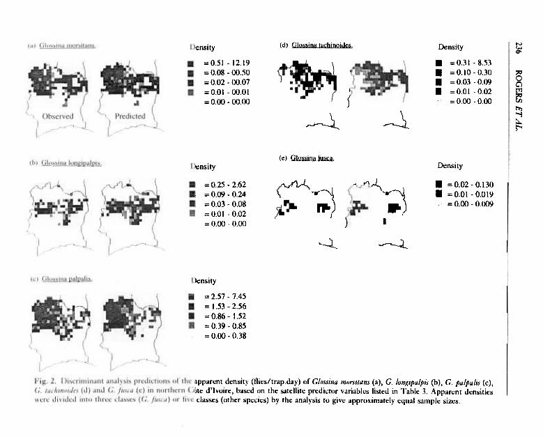
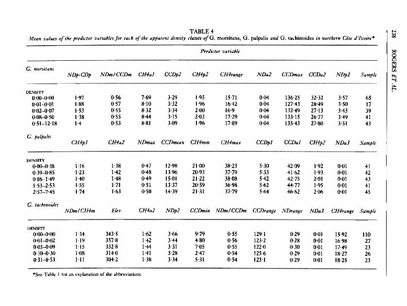
Figure 2 (a-e) shows the observed andpredicted abundance classes of the five speciessampled in the north of Cote d'Ivoire andTable 3 lists the predictor variables used andthe accuracy of the predictions. Given therelatively small ranges of density in each class,the results are surprisingly good. Table 4 liststhe mean values of the predictor variablesfor the five density classes for each of thethree most widespread species, G. morsitans,G. tachinoides and G. palpalis. In many casesthere is a gradual, monotonic increase ordecrease in the mean values of the predictorvariables across the density classes. Only veryslight differences between the predictor vari-ables are found in areas of absence or presenceat the different densities.

satellite imagery and the development of novelimage-processing and analytical techniques allcontribute to an increasing ability to predictthe distribution and abundance of naturalresources and disease vectors using remotely-sensed, satellite imagery. The success of theapproach described in this review is all themore remarkable when the relatively poorquality of the distribution data is remembered,together with the long periods of time overwhich they were recorded. The satellite datawere gathered during the 1980s, when particu-larly severe droughts affected much of thestudy area, resulting in rapid changes of thedistributional limits of some of the speciesconsidered. Glossina tachinoides, for example,extended its range south, and apparentlyreplaced G. palpalis over large areas of centralCote d'Ivoire (Clair, 1987; DJR, unpubl. obs.).Curiously, and perhaps significantly, wheneach data-set is kept separate within theanalysis, the predicted area of suitability forG. tachinoides shifts southwards into the samecentral and southern regions of Cote d'Ivoirethat the species invaded in the 1980s. These flyadvances may be facilitated by only slightchanges in the average environmental con-ditions in the newly invaded areas. Forexample, the present analysis indicates that thedifference between the mean NDVI in sites ofpresence or absence of G. tachinoides variesbetWeen -0.08 and +0.04 (in COte d'Ivoireand Burkina Faso, respectively), each asmall fraction of the total range shown bythis variable across these two countries (0.53;Table I). l'\S some areas become more suitablefor flies, however, other areas become lesssuitable, so that the distributional limits shiftslowly with time. The expansion and subse-quent contraction of tsetse-fly distributionshave been previously recorded, but globalenvironmental change will bring about perma-nent range shifts in addition to these relativelyshort-term variations.

.\s more predictor variables are added intothe analysis, the predictions tend to becomemore accurate (Table 2) and more well-defined, so that with 10 predictor variablesthe analvsis identifies areas of suitabilitv witheither ~ relatively high or relatively low

~

DISCUSSION;~;(I~~J~~~'.~~~"::,;\~~i(e

Advances in micro-computing technology,the increasing availability of remotely-sensed,

~-~.

::"..~e,

~~"=~~.~-.~...'"",....::'"''"',...

~.,.~~~~~,~~~.,.~~~~'"~..,. ~~

~,~

.~

N"",t:~

"",~

...~

:~~

~-

;'-~~

t""'~"~

'"~

"'=.

~

';:

.;::

~,...

~

:§~"~",...t:'"'

~~~~.

::'"~~,.t:~'"...~~.;:~.".~,.~~.".E-~~E~"..,~

~< SA

TE

LLITE

D

AT

A A

ND

TS

ET

SE

-FLY

DIS

TR

IBU

TIO

NS

c C

"""- "-"

Co."

" ..f'". ,,""'

8~xQ

O88Q

~~

uzuzZuuz:tu

u u

Ecc~

~ N

-~.-:c""

~ ~

N

E~

~E

EU

~

Q~

Qrt:C

~~

E:c8u:c

ZU

UU

uQU

uuuZ

,,~bD... -.~

~~

..."

~

~

N

~~

U

C

o" "

~

N

-.-

~E

:t~~

:tO~

~~

'CO

UZ

'CU

Z""'C

UZ

U

c.."'"~

~

..CN

N_-~

~~

~o505e~

~;I:O

XUuuuu

uooouZ

u uuuuzz

ec:C

:" C

:Q.-~

~

N'"

N .., -~

u

~~

~ii8~

8~~

:.;a~uuuuu'd~

z

..'t"><

C

~N

_C"',,"

><

to;

Po.

, ~

C

Q't"cU

~C

"CP

o....,~

,..,'O,..,Q

OO

~uuz~

~8zzzo

Z

~

c:.. -;

E~

c'"' '-t"

C

'-t"

C.euN

X~

..., ~

NX

~O

b.Q~

OQ

E~

~X u

;jOz-;;jz

zOu

EZ

OO

Z

Z

-N...,'ot",,",-C

r-..~Q

-:

=~

~~

=.:..c~

.,.,~

=cc:o

.,.,-c

Q~

""~Q

':"c~

~~

~~

~-Q

CC

~-

.,.,~~

~~

""QC

C:O

~-

r-.r-.~

r-.

~-Q

C:O

Cr

.,.,'"~

r-.r-.""-C

C:O

r ",r-.

~.

r-.-CC

"'.~

~~

-QC

C~

-

~~

.,.,r-.QC

C~

-.,.,r-.~

~~

""-CC

:O~

-"'.,.,~

.cC

Cr

"'.c~

'"=

~

c:oc:or

~:;?

-CQ

.C:O

C-C

"'.

=.~r-.

r-..~C

C~

~.c

~-C

-CC

C~

.,.,~~

'"

r-.r-.-CC

:OC

:O~

~.~-C

-~-C

:OC

r r-.~~

'"r-..,.,-C

:OC

:O-C

~

.

g::,~-C

C~

.r-.~

.C:O

C:O

-C""

--C~

."'-.c:oC-C

""~

'"~

.

:$M"'C

:OC

:O, ##" "

,...»C

'- .-C

" .~

..>

, >

,~

I/OW

J"""g,

" ...>

U

~

U

C ':'

~U

" "

" ~

..'"

'" I/O

u

~'O

;~

~U

U~

~C

I;CI;

~

0:0-~

~

.-. .

~

..;c.=~.~"oS.Q.."of'-0c.=~c.."Q

."";..E"~roo""C/).

235

" O

JC

O

J"'" _C

bD""',

bD:t N

--~

'-5C

OJ~

cU~

""- "

~5~

~55~

§§§z

:§:

236

'~I~.=0(5:§:

...,00\<"1

8~

r"\00

acioooo,

O\or---

g-01"\00

~gggg

, ,

., ,

-~N

-8

01"\000~

00000

";n II

II II

II II

c8

RO

GE

RS

ET

A

L.

rt;,

~

:1

.~

\C

o

~v

1r

i \0,

'1

J~~0a~

;!j-;;0:..9~S~0ae: 2=

'";nc8-:;;..~c8

~ ~s<'I-q-~

<'IO

-0<'1000

MO

OO

O,

,.,.,a ,-0<

'1000000000\I

\I \I

\I \I

00\~fO

"I-x-0-,000

..

N-

800000

II II

II..

~"-'~(61'-.

-

.-r-,I111

j~

II"\\ON

II"\~""II"\II"\~

""r.:M

":OO

, ,

,r--

\0 C

\8II"\II"\~

""?;-

M":O

OO

';n II

II II

II II

c.8

j

1'""

, '"

~-:

.., -;n:-::

c~

..

~~~

--~

c'"-~

~

Co-'

;-~,c.

---c.~~

c.

.., -E

~...,~..

~--

~~

,..~

,co =

=~

-~~

. ~

-c--->

,

Co-'~

~..-~

- co

---"'~co --C

--:;: -;;;

-..~

..0

~

-~c.

~

,.. c.

'" ---~

~ ,..

", ~ ~

:: !on

--~'" '"

w

~~

:C

o-' ~-;n

'- c.~

o..co-c

>,-

-.co~

"~

-~-co -.

c.",-co..>

,=

~oC

,, '" '"

..c..--::---'"~

~"

" c.

>'"""

-~

~...

"'oCc

~1

.." -~

...0

--=-

c ~ '"

"-,,...' '"co~

'"0.

CO

c.:!,~C

O -0"

"

~'-'..

-5 c-.l:

'- ~ ..~w

~-

"' C ~

::

0Cw

..,

--~uc'-.~

""

.."-c.""'",

~

..-~

~ ~

>'~

..:!",C

O

-

cCo-'"

CO

..

-~..

Cc~

~

~

-

c~o

-:e 3-5-c

'""",~",:-:0"

---~'"'

~--

'-' :: ..-~

~N

~'"

"biI-..-..~

"'~

-0"'-8

"'-00>

- .~

0

0 0

0 0

~

II II

II II

II

8

SATELLITE DATA AND TSETSE-FLY DISTRIBUTIONS 237

T.I\BLE 3The 10 most important predictor variables used to tkscribe the apparent densilJ' of tsetse (flies/trap. day) innorthern Cote d'/voire, and the accuracy of the predictions ~r the abundance classe.( (five for all species except

G. fusca)+

G. longipalpisG. morsitans

Spec;e.( of Isel.(e fly

G. tachinoide.{ G. fusca

RANK1234

NDP-CDpNDm/CCDm

CH4alCCDp2CH4p2

CH4rangeNDaZ

CCDmaxCCDa2NDp2

CCDa2Cffial

NDP-ffipCH4a2Cffip2

NDaI/CH4alCH4minCCDa3

CH4meanCCDp3

CH4p3CH4a2NDmaxCCDa3CH4minCH4maxCCDplCCDaI

CH4p2NDa.,

NDrn/GI4mElev

GI4a2NDp2

CCDminNDm/Cffim

CffirangeNDrange

NDaJGI4range

CCDa2CH4a2NDplCH4alElev

CCDp2CCDmin

CCDrangeNDpl-CH4pl

NDmax

89

10

Densiry and /arcurat:J' of prediction (%)]

o.OO-().oo (58)0.01-0.01 (100)0.02-0.07 (72)0.08-0.50 (51)0.51-12.2 (63)

O.OO-O.()() (81)0.01-0.02 (80)0.03-0.08 (76)0.09-0.20 (94)

0.25-2.62 (83)

0.00-{).38 (78)0.39--{}.85 (50)0.86-].49 (30)].53-2.53 (59)2.57-7.45 (58)

O.OO-{).()() (65)0.01-{).02 (78)0.03-0-09 (78)0.la-o.30 (62)0'31~'53 (65)

O-QO-{)-OO (98)0'01-0-01 (100)0'02-0-13 (100)

.See Table 1 for an explanation of the abbreviations

probability; and intermediate probabilities (i.e.within the range 0.35-0.65) are ven. scarce(Fig. I). With the exception of G. palpalis, thepercentage of false positives (i.e. false predic-tions of presence) always outnumbers thepercentage of false negatives (false predictionsof absence), often considerably (Table 2 andFig. I). The former indicate areas of apparentsuitability for flies that are not occupied bythem, or in which flies were not recordedby the surveys. This is a feature of manydistribution maps (i.e. species do not alwaysoccupy all areas that are suitable for them, orare not always found, even when they occurthere). False-negative predictions, however,indicate a more serious situation where thetechnique, for one reason or another, has failedto define the full range of conditions in whichthe flies can survive. The percentage of falsenegatives is highest (8%) for G. palpalis, themost widespread species, and the errors arise

because the analysis fails to identify its re-corded northern limits in Burkina Faso [Fig.l(c)]. The same environmental changes thatcaused a southward extension of G. tachinoidesmay, however, -have caused a retreat of G.palpalis (a species adapted to moister con-ditions) from the northern part of its range,thus explaining the high error rate.

Whilst the ability to describe the training-set data is the first criterion for a successfulstatistical description of a species distribution,the technique is only of real use when it can beused to describe distributions in other places,and at other times. The maps presented inFig. 1 show predicted distributions of thestudy species in Ghana and Togo. The predic-tions for Togo sho\\ both similarities anddifferences with the recently mapped tsetsedistributions in this country (Rogers et al.,1994; Hendrickx et al., 1995). Predictions forG. palpalis and G. tachinoides are rather better

~~

238.~~~=.::s

",~~~..."~'-=~~~onu"0'0c:E'"ac.:j

"'"~'=,~-;Q,

-;Q,

c.:j

'"c~'~..~e..,.c.:j

~~

...J~

t

< ~

f-.~'"':0.-...'~~

~~~'=~'="~~~'"''="...,~-...,~.c,'=t:'=~...~~~<

'-."~~t~~~~'=

~

~""'~t:~..~~~~ RO

GE

RS

E

T

.,-fL.

~::g~~EI.,:) ~u~~ -'"~u~e"'-

~ '"~""'""'

'"~~ ~~~u '"'3

~ '"~~..~su '"~~ ~~~'3'-"1

~""""""M

""""""""""00000

O\O

N~

-~

-""~~

r:.. 00 0000 00

o-N-ot-U

"lo-N

...,...,-OM

MM

MM

""-CO

M-C

o-o-OO

Q\

~~

NN

~

-N

Q\Q

\t"ot"Q

\N«)

~~

~tt

~:;?-r--o--'00""

N

,.-""qi"'~

-N~

-~

~??9~

ZO

OO

OO

'"Q

r.-.~"'~

~~

~~

"?"

~"'""'"~

"'"_00_066666

""M~

""MN

-t"-t"--t",0 r'N

M

.i-,M

NM

MM

Na-M

r--C"".-r--~N

~~

-Q~

MN

NN

N

r-.QM

~-

""""1'""1'"'"..;.,..;.,..;.,..;.,..;.,

1r)('-.Q\-r-,

-Q-r-,'f"'f"

...,~~,..,.,\S "",:.~u '"'3

:t:\oJ ~E"to

a~~

~u..~~ '"~E"1-~"" ~uu ~s~ '".::-~ ,.,~:co;

~E'~r...,

~."=

,,

~'t"""t"

~.6~N

r:.. ~

I

I I

I e-

=--o

r-

~ .~

~

'!' ~.

ZO

OO

-No.JQ ~

N~

-M~

~~

r:--~

~-c-r--=

,=

'='0""""

NM

';'M+

O""N

~-

O~

N""'"

~6~

6~N

NN

NN

MQ

\~~

Q\

Nr--O

Q\r--

Q()r:.Q

()-c.r:.M

MM

MM

-c ::>

U

") -.to

~'":'~

~r:-

r--.~a--Q"."

00000

0 ""N

N-ot-

""""-ot--C-C

.;., .;., .;., .;., .r.

a-N"",",N

O-.c,",,",-.c

N':'N

.,f-.:c~

~~

~~

N"""""'-C

Q\Q

\OQ

\O":"':'N

":'N

0000066666

-NM

-'"-to-to-to-to-to

~~~~~~

~~,..,u~~ ;:.~... '"~"t-

a '"~~ '"~~:<:

'"~~suSu"-~~~uU "'"'~

~ ~E''3

"J~~~~'""

xN~

O""

_00...,'"

~~

~~

~~

'" ZOO

OO

O

~

~.,.~

-~

. -:- -:- ? -:-

U"I~

~O

NM

r:..N+

+"'U

"I""-O...,...,...,...,...,

NN

-.r-~'9";t"";t"";t"~

-c..".-~..".

-C""'M

NM

MM

MM

M

QoO

ll'lr-.-r-.~

O'-t"'"

ci-+r:.";".;,

-NO

-o-Q

.";'N.;,";'

NN

NN

N

...,~...,"t-"t-

...,...,...,...,...,66666

Q-O

OO

Q-=

'N

NM

NN

66666

0000066666

N(X

)Q\t"-U

"IQ

\Q\",,"N

N

';",cr:..~~

O,

,-C..,

-NN

NN

-

.;.§';;:".E~,."-5"0,§E;0"E

o""c,...-":c;~:IJ.

S.\TELLITE DATA A1'.'D TSETSE-FLY DISTRIBUTIONS 239

NDVI and CCD variables appear 10 and sixtimes, respectively (some combination of thesevariables making up the remainder). Consider-ing only those species for which the abundancedata are also available, the figures become 14for thermal, six for NDVI and two for CCDdata. Thermal-channel data also predominatein describing the abundance data, but less sothan for the distribution data (with nine, threeand seven occurrences for the thermal, NDVIand CCD data, respectively). The low import-ance of the CCD imagery in determiningdistribution and its relatively greater import-ance in predicting abundance indicates thatfly distribution limits in this part of Africamay be more sensitive to temperature, whilstabundance within the distributional limits issome function of rainfall, which determines

vegetation growth.

COND...USIONS

than those for G. morsitans and G. longipalpis,although there has also been a southwardextension of G. tachinoides in Togo that is notpredicted by the present analysis, and does notappear on previous maps for tsetse in Togo(Ford and Katondo, 1977). Clearly, therefore,the distribution of tsetse in Togo, and presum-ably elsewhere, has changed from the historicalpicture that forms the basis of much of thepresent analysis and, in the light of recentenvironmental changes in Africa, it is unlikelythat non-contemporary satellite data will givean entirely satisfactory fit. The ideal approachto tsetse mapping is therefore to use contem-porary satellite and fly-distribution data todefine the areas of suitability for each tsetsespecies and, from this, to make predictions forother places and times.

A further complication arises from the ad-aptation of each species to local conditions,about which very little is known at present.Species such as G. morsitans, and even itssubspecies, occupy vast areas of Africa (e.g.greater than 400 of longitude for G. m. submor-sitans) and almost certainly show biologicalvariation across such distances. Behaviouraland ecological differences within G. pallidipes,a widespread species in East and southernAfrica, have. already been shown (Rogers,1990; Baylis and Nambiro, 1993). These effectsmean that the characterization of a species'habitat in one area may not easily be extendedto other, remote areas. Given contemporarysatellite and distributional data, however, theapproach suggested may be used to estimatethe degree of difference in habitat types acrosswide geographical areas. Whilst satellite datamay not immediately explain within-speciesdifferences across large geographical areas,they may, in the first instance, illuminate suchdifferences and hence lead to a better biologicalunderstanding of them.

Of the three main satellite data types used inthe present analysis (NDVI, A VHRR-channel-4-bri!!,htness temperature and CCD imagery),the tht:rmal channel data appear most fre-quently in the predictor variables for fly distri-bution. On 19 occasions, one or other thermalvariable is in the top five predictor variables forthe eight species of tsetse considered, whilst

It is clear that remotely-sensed satelliteimagery can be a powerful tool in our abilityto investigate large-area phenomena such asthe distribution and abundance of the insectvectors of disease. The application of temporalFourier processing to multi-temporal, meteor-ological, satellite imagery allows characteriz-ation of habitat 'fingerprints' in the form ofmeans and the seasonal timing and seasonalextremes of values of temperature, rainfalland vegetation surrogates. Insect-vector distri-butions clearly depend on habitat types and soshould be amenable to statistical descriptionsbased on such habitat fingerprinting. In future,satellites giving data with higher spatial andspectral resolution will provide a much morefine-grained view of natural habitats (Hayel al., 1996) and it is timely to prepare now forthe wealth of new data these satellites will

provide.A statistical description of a tsetse-fly habi-

tat or distribution is, however, no substitutefor a full, biologically based understanding ofthe same phenomenon. Such an understandingcomes from a study of the underlying demo-graphic processes but, as explained elsewhere(Rogers and Randolph, 1993; Randolph, 1994),

ROGERS ET AL.240

the information on such processes is oftenlacking, leaving the statistical approach as theonly one available at present. The long-termaim of the present work is to produce riskmaps for tsetse-borne diseases based on asound biological understanding of epidemio-logical processes. Satellite imagery provides away of revealing the patterns in epidemiologi-cal processes from which such an understand-ing will eventually arise.

(GIMMS) group at the National Aeronauticsand Space Administration (NASA) GoddardSpace Flight Center (GSFC) during work (byS.I.H.) towards a NASA Planetary BiologyInternship. The NDVI and Meteosat datawere kindly supplied by F. Snijders of theARTEMIS project at F AO, Rome. DrsG. R. W. Wint and S. E. Randolph kindlyread and commented on the manuscript. Thiswork is funded by a grant from the OverseasDevelopment Administration (ODA), U.K.,under the Livestock Protection Programme(R5794) and administered through the NaturalResources Institute (NRI).

ACKNOWLEDGEMENTS. The channel-4-brightness-temperature data were supplied byDrs C. Tucker and C. Justice of the GlobalInventory Monitoring and Modelling Systems

REFERENCES

A.-.oRES, L., SALAS, W. A. & SKOLE, D. (1994). Fourier-analysis of multi-temporal AVHRR data applied toland cover classification. International Journal of Remote Sensing, IS, 1115-1121.

ANON. (1982). Cartographie de la Repartition des Glossines. Maison-Valfon, France: Institut d'Elevage et deMedecine Veterinaire des Pays Tropicaux (IEMVT).

BAYLIS, M. & NA.\lBIRO, C. O. (1993). The responses of Glossina pallidipes and G. long.pennis (Diptera:Glossinidae) to odour-baited traps and targets at Galana Ranch, south-eastern Kenya. Bulletin ofEntomological Research, 83, 145-151.

CHALLIER, A. & LAVEISSIERE, C. (1973). Un nouveau piege pour la captUre des glossines (Glossina: Diptera,Muscidae): description et essais sur la terrain. Cahiers ORSTOM, Serie Entomologie, Medicale et

Parasitologie, 11,315-317.CHATFIELD, C. (1980). The Analysis of Time-series: an Introduction. London: Chapman & Hall.CLAIR, M. (1987). Donnees recentes sur la repartition des Glossines au Niger, au Burkina Faso et en COte

d'Ivoire. In International S,"ientific Council for Trypanosomiasis Research and Control (ISCTRC), 19thMeeting, Lome, Togo, 1987, pp. 345-350. Nairobi: Organization of African Unity.

EASTMAN, J. R. & FULl(, M. (1993). Long sequence time-series evaluation using standard principalcomponents. Photogrammetric Engineering and Remote Sensing, 59, 991-996.

FAIRBAIRN, H. & CULWICK, A. T. (1950). Some climatic factors influencing populations of Glossinaslllynnertoni. .4nnals of Tropical Medicine and Parasitology, 44, 27-33.

FoRD, J. & K\TONDO, K. M. (1977). The Distribution of Tsetse Flies in .4frica. London: Hammond & Kell.FoRD, J. & LEGGATE, B. M. (1961). The geographical and climatic distribution of trypanosome infection

rates in G. morsitans group of tsetse-flies. Transa,.tions of the Royal Society of Tropical ,Wedicine andHygiene, 55, 383-397.

GASCHFN, H. (1945). Les glossines de l'Afrique Occidentale Francaise. .4cta Tropica, 2 (Suppl.), 1-131.GREEN, P. E. (1978). Analyzing ,Wultivariate Data. Chicago: Dryden Press.HAY, S. I., TuCICEK, C. J., ROGERS, D. J. & PACKER, M. J. (1996). Remotely sensed surrogates of

meteorological data for the study of the distribution and abundance of arthropod vectors of disease.Annals of Tropical jl-fedicine and Parasitology, 90, 1-19.

HL~RICK.X, G., ROGERS, D. J., NAPALA, A. & SLINGL'lBERGH, J. H. W. (1995). Predicting the distributionof riverine tsetse and the prevalence of bovine trypanosomiasis in Togo using ground-based andsatellite data. In International Scientific Council for Trypanosomiasis Research and Control (ISCTRC),22nd ,Weeting, Kampala, Uganda, 1993, pp. 218-227. ~airobi: Organization of African Unity.

HILL, M. O. (1991). Patterns of species distribution in Britain elucidated by canonical correspondenceanalysis. Journal of Biogeography, 18, 247-255.

SATELLITE DATA AND TSETSE-FLY DISTRIBUTIONS 241

I.

t

I

Hol..B~, B. ~. (1986). Characteristics of maximum-value composite images from temporal A \'HRR data.International Journal of Remote Sensing, 7, 1417-1434.

LAMBN, E. F. & EHRLlrn, D. (1995). Combining vegetation indices and surface temperature for land-covermapping at broad spati;il scales. International.10urnal of Remote Sensing, 16, 573-579.

LAMBN, E. F. & EHRLlrn, D. (1996). The surface temperature-vegetation index space for land-coverchange analysis. International Journal ~r Remote Sensing, 17, 1-15.

LAVEISSIERE, C. & CHALLJER, A. (1977). La Repartition des Glossines en Haute-f/olta, Canes Ii JI2()(K)()(K).Notice Explicative No 69. Paris: Office de la Recherche Scientific et Technique d'Outre-Mer.

LAVEISSIERE, C. & CHALLJER, A. (1981). La Repartition des Glossines en Cote d'Ivoire, Cartes Ii J 12 ()(K) ()(K).Notice Explicative No 89. Paris: Office de la Recherche Scientific et Technique d'Outre-Mer.

LARK, R. M. (1994). Sample size and class variability in the choice of a method of discriminant analysis.International Journal of Remote Sensing, 15, 1551-1555.

Los, S. O. (1993). Calibration adjustment of the NOAA A\'HRR normalized difference vegetation indexwithout recourse to component channel I and 2 data. International Journal of Remote Sensing, 14,1907-1917.

OLSSON, L. & EKLUNDH, L. (1994). Fourier series for analysis of temporal sequences of satellite sensorimage~.. International Journal of Remote Sensing, 15, 3735-3741.

MARRIOTT, F. H. C. (1974). The Interpretation of Multiple Obsel'Vations. London: Academic Press.PRINCE, S. D., JUSTICE, C. O. & Los, S. O. (1990). Remote Sensing of the Sahelian Environment: a Rerie/P of

the CuI"Tent Status and Future Prospects. Ispra, Italy: Technical Centre for Agricultural and Rural

Development.RANDOLPH, S. E. (1994). Population dynamics and densif).-dependent seasonal mortalif). indices of the tick

Rhipicephalus appendiculatus in eastern and southern Africa. Medical and r'eterinaIJ' EntomologJ', 8,351-368.

ROGERS, D. J. (1990). A general model for tsetse populations. Insect Science and its Applications, 11,331-346.ROGERS, D. J., HENDRlCKX, G. & SLINGENBERGH, J. H. W. (1994). Tsetse flies and their control. Ret'Ue

Scientijique et Technique de /'Office International Epizooties, 13, 1075-1124.ROGERS, D. J. & RA.-.DOLPH, S. E. (1986). Distribution and abundance of tsetse flies (Glossina spp.). Journal

of Animal Ecology, 55, 1007-1025.ROGERS, D. J. & RA.-.DOLPH, S. E. (1991). Mortality rates and population density of tsetse flies correlated

with satellite imagery. Nature, 351, 739-741.ROGERS, D. J. & RANDOLPH, S. E. (1993). Distribution of tsetse and ticks in Africa, past, present and future.

Parasitology Today, 9, 266-271.ROGERS, D. J. & WILLIAMS, B. G. (1993). Monitoring trypanosomiasis in space and time. ParasitologJ'. 106

(Suppl. I), S77-S92.ROGERS, D. J. & WILLIAMS, B. G. (1994). Tsetse distribution in Africa, seeing the wood and the trees. In

Large-scale Ecology and Consel'Vation BiologJ', eds Edwards P. J~, May, R. M. & Webb, N. R.pp. 249-273. Oxford: Blackwell Scientific.

SNljDERS, F. L. (1991). Rainfall monitoring based on Meteosat data-a comparison of techniques applied tothe western Sahel. International Journal of Remote Sensing, 12, 1331-1347.

TATSUOKA, M. M. (1971). Multivariate Ana~ysis: Techniques for Educational and Psychological Research.New York: John Wiley & Sons.

TER BRAAK, C. J. F. (1986). Canonical correspondence-analysis-a new eigenvector technique formultivariate direct gradient analysis. Ecology, 67, 1167-1179.

To\\'NSHE.~, J. R. G. & JUSTICE, C. O. (1986). Analysis of the dynamics of African vegetation using thenormalized difference vegetation index. International Journal of Remote Sensing, 7, 1435-1445.

VERHOEF, W., MENENTI, M. & AzzALI, S. (1996). A color composite of NOAA-A VHRR-NDVI based ontime-series analvsis (1981-1992). International Journal of Remote Sensing, 17,231-235.

WILLIAMS, B., ROGw, D. J., STATON, G., RIPLEY, B. & BOOTH, T. (1992). Statistical modelling ofgeoreferenced data: mapping tsetse distribution Zimbabwe using. cli~ate and. vegetation data. InModelling Vector-borne and other Parasitic Diseases, pp. 267-280. Nairobi: International Laborato~. forthe Research into Animal Diseases (ILRAD).