HAL Id: hal-03004809https://hal.archives-ouvertes.fr/hal-03004809

Submitted on 13 Nov 2020

HAL is a multi-disciplinary open accessarchive for the deposit and dissemination of sci-entific research documents, whether they are pub-lished or not. The documents may come fromteaching and research institutions in France orabroad, or from public or private research centers.

L’archive ouverte pluridisciplinaire HAL, estdestinée au dépôt et à la diffusion de documentsscientifiques de niveau recherche, publiés ou non,émanant des établissements d’enseignement et derecherche français ou étrangers, des laboratoirespublics ou privés.

PREDICTING TECHNOLOGY SUCCESS BASED ONPATENT DATA, USING A WIDE AND DEEPNEURAL NETWORK AND A RECURRENT

NEURAL NETWORKMarie Saade, Maroun Jneid, Imad Saleh

To cite this version:Marie Saade, Maroun Jneid, Imad Saleh. PREDICTING TECHNOLOGY SUCCESS BASED ONPATENT DATA, USING A WIDE AND DEEP NEURAL NETWORK AND A RECURRENT NEU-RAL NETWORK. IBIMA 33, 2019, Granada, Spain. �hal-03004809�

PREDICTING TECHNOLOGY SUCCESS BASED ON PATENT

DATA, USING A WIDE AND DEEP NEURAL NETWORK AND A

RECURRENT NEURAL NETWORK

Marie SAADE

Laboratoire Paragraphe (EA 349), Université Paris 8 Vincennes-Saint-Denis, Saint-Denis, France,

marie.karam@etud.univ-paris8.fr

Maroun JNEID

TICKET Lab., Antonine University, Hadat-Baabda, Lebanon, maroun.jneid@ua.edu.lb

Imad SALEH

Laboratoire Paragraphe (EA 349), Université Paris 8 Vincennes-Saint-Denis, Saint-Denis, France,

imad.saleh@univ-paris8.fr

Abstract

The temporal dynamic growth of technology patents for a time sequence is a major indicator to measure

the technology power and relevance in innovative technology-based product/service development. A new

method for predicting success of innovative technology is proposed based on patent data and using Neural

Networks models. Technology patents data are extracted from the United States Patent and Trademark

Office (USPTO) and used to predict the future patent growth of two candidate technologies: "Cloud/Client

computing” and “Autonomous Vehicles”. This approach is implemented using two Neural Networks

models for accuracy comparison: a Wide and Deep Neural Network (WDNN) and a Recurrent Neural

Network (RNN). As a result, RNN achieves a better performance and accuracy and outperforms the WDNN

in the context of small datasets.

Keywords: Innovative product development, forecasting technology success, patent analysis, machine

learning.

Introduction

Product development consists of methods and processes focused on value creation through the development

of new and innovative technology-based products. The traditional technical aspects are involved such as

engineering design techniques, cost reduction, increase in product quality, etc. However, predicting

technologies success is a crucial need and a prerequisite step for investments in product development and

value creation. For instance, (Jneid & Saleh, 2015) have stated that for start-ups facing a competitive

environment, innovation is a key factor contributing to their success. They presented a new approach based

on co-innopreneuriat which provides a method for co-innovation and co-creation of values by convergence

and collaboration. Furthermore, organizations seek to enhance the Research and development (R&D)

activities by increasing the R&D investments on new patents technologies (Hall, 2004). Technology patents

can be used as a significant factor for measuring success and relevance in technology-based product

1

development, and therefore, patents growth of a technology can be used as a major indicator to predict its

power and its impact on value-creation.

Accordingly, the main problematic of this study is to examine how technology success can be forecasted

based on patent analysis, using a convenient prediction tool while considering data availability and how to

prioritize several trending technologies in order to identify the most appropriate ones for a given investment

project.

Therefore, in this paper, we initially propose a novel model for forecasting technology success and

predicting patents growth, based on two Neural Network models for comparison purpose: a Wide and Deep

Neural Network and a Recurrent Neural Network. Noting that according to our research, this approach has

not been implemented so far when forecasting patents growth in this specific context.

Literature review

Technologies Patents play a critical role in fostering innovation and making decisions (Chen, et al., 2017).

Patents data can be used and analyzed to predict promising technology, in order to provide reliable

knowledge for decision making (Cho, et al., 2018). Patent expansion potential and patent power are

considered as technology scope indicators (Altuntas, et al., 2015). In addition, the National Science Board

highlights the importance of patents counts and patents citations (National Science Board, 2014) in

measuring the innovation value and the knowledge flows. Professor Bronwyn H. Hall (Hall, 2004)

identified a positive correlation between the patents grant growth and the industrial R&D, which

consequently increases the total R&D.

Patent-based technology forecasting methods:

Patent-based technology forecasting has been considered a reliable method for finding technology scope,

identifying trending technologies and improving decision-making.

For instance, a patent analysis has been elaborated to quantitatively forecast the technology success in the

context of patent expansion potential, patent power, technology life cycle and diffusion potential (Dereli &

Kusiak, 2015). Cho, Lim, Lee, Cho and Kyung-InKang analyzed patents data to predict promising

technology fields in the building construction (Cho, et al., 2018).

In addition, patent data have been employed in a matrix map and in the quantitative method ‘K‐medoids

clustering, in order to predict the vacant technologies in the management of technology field (Jun, et al.,

2012). Furthermore, a machine learning approach has been proposed to detect new technologies at early

stages, using several patent indicators and a multilayer neural network, while focusing on the

pharmaceutical technology (Lee, et al., 2017). Kim and Lee proposed a prediction approach for multi-

technology convergence based on patent-citation analysis, a neural network analysis and a dependency-

structure analysis (Kim & Lee, 2017).

Research design

In the present study, the analysis of patent data is considered as a quantitative approach to assess its impact

on a technology’s success. Specifically, this study forecasts the future growth of patents for a given

technology, using a Neural Network model. The latter is built using two separate methods for comparison

purposes: a Wide and Deep Neural Network (WDNN) model and a Recurrent Neural Network (RNN)

model.

Neural Network model:

2

The artificial neural networks are used for a dynamic (ALSHEIKH, et al., 2014), unsupervised learning

(Schmidhuber, 2015) from historical data in order to estimate future values.

In this paper, the neural networks are used specifically for data classification, regression, data analysis and

prediction.

Wide and Deep Neural Network model:

Generally, the more data a Neural Network can have, the more its generated predictions are accurate and

reliable (Thrideep, 2017). However, Big Data analytics issues and challenges can be referred to the fast

information retrieval, data representation, data processing, etc. For this reason, this Neural Network is

structured as a wide and deep model in order to support such tasks, since it can handle complex large-scale

data (Elaraby, et al., 2016), integrating heterogeneous input data (Najafabadi, et al., 2015). In addition,

Deep learning algorithms generalize the extracted representation and the relationships in the data, by

exploring new or rare features combinations by transitivity of correlations. However, deep neural network

can over-generalize and extract less relevant features (Cheng, et al., 2016). For this reason, the

memorization of features interactions or correlations in the historical data, the exception rules and the

frequent co-occurrence of features is a crucial need to enhance the neural network prediction. Hence the

importance of merging a wide linear model for learning exceptions and memorizing specific rules with a

deep model for learning interactions within historical data and then generalizing the output on new data

(Cheng, et al., 2016).

Recurrent Neural Network model:

RNN is a model of artificial Neural Network where its nodes are connected along sequences. Accordingly,

the main reason of using this model of Neural Network is to process sequences of inputs in order to predict

a sequence of outputs where theses sequences can be different in lengths for different technologies (Ng, et

al., 2018), which is applied in our case as well.

In addition, Gated Recurrent Units (GRU) are employed in the RNN as they tend to optimize the

performance on smaller datasets (Chung, et al., 2014), which is the case of our study where the data are

limited to 163 records.

The above models will be discussed in details in the following sections: Proposed methodology and Neural

Network models structures.

1. Proposed methodology

The proposed methodology is illustrated with a process flow, as presented in Figure 1, covering the

following main objectives: data collection, database integration, data manipulation, datasets creation,

neural networks implementation, results visualization/analysis and decision-making.

It consists of 15 steps, explained in Table 1:

3

Figure 1: Methodology design.

Table 1: Methodology design steps.

Objective Step Description

Data Collection Step 1 Searching for old and new trending technologies from several references.

Step 2 Listing the related keywords for each technology.

Database

integration

Step 3 Inserting these technologies’ data and their related keywords into two

separate tables in a new integrated database. These two tables are related

according to the identifier “tech_id”.

4

Noting that these tables are considered as dictionary tables which the

following steps will depend on.

Data Collection Step 4 Extracting patents data related to each technology from a patent database

based on keywords matching. Several patents databases could be used

such as the United States Patent and Trademark Office (USPTO)

database. This latter is considered among the richest intellectual property

databases, it issued approximately 10 million patents so far (USPTO,

2018).

Database

integration

Step 5 Manipulating and inserting data into the integrated DB.

Data

manipulation

Step 6 Computing the total number of patents per technology per year.

Datasets

creation

Step 7 Querying and grouping the data by year following the axis: [Year-max, … ,

Year-1, Year0, Year1, … , Yearp]. Such as:

- max: represents the maximum number of years per technology where

historical data is available in the training dataset.

- p: represents the number of years for which we are validating results

in the testing dataset, and the number of years for which we are

predicting results in the prediction dataset.

- Year0: represents the most recent year in the training data set per

technology, based on data availability.

Neural networks

implementation

Step 8 Training the Neural Networks.

Step 9 Testing the Neural Networks.

Step

10 Predicting the number of patents.

Step

11

The number of years y that we need to generate is checked at every step

during the prediction phase until y is equal to p.

Database

integration

Step

12

Inserting the output data of the Neural Network into the integrated

database.

Results

visualization and

analysis

Step

13

Illustrating the patents variation in statistical graphs.

Step

14

Ranking the candidate technologies based on their patents progress.

Decision-making Step

15

Evaluating and prioritizing the candidate technologies based on the above

ranking and based on business perspective.

2. Neural Network models structures

The Neural Networks have been built using the TensorFlow software library under Python. Tensorflow is

a high level open-source API created by Google and is used for Machine Learning and deep neural network

purposes (TensorFlow, 2018). As previously mentioned, two Neural Network designs are proposed based

on different models:

5

2.1. Wide and Deep Neural Network

This Neural Network structure is based on the “DNN Linear Combined Regressor” (TensorFlow, 2018).

Noting that “regression” refers to the prediction of a continuous variable as output (Bishop, 2006), in our

case, the estimation of the number of patents.

Furthermore, Adagrad is used as an optimization method during the training phase, since it can handle

sparse data (Ruder, 2016) and enhance the robustness of the Stochastic Gradient Descent (Dean, et al.,

2012).

This Neural Network consists of the following layers:

Figure 2: Wide and Deep Neural Network.

Input Layer: The input layer is composed of two types of nodes:

- Continuous number: represents the number of patents for a technology for each available

year.

- Bucket: represents ranges of the same data as the continuous number for each available

year.

Hidden Layers: represent the intermediary layers that can make the model more adaptable. This

neural network contains a specific number h of hidden layers, and each one contains a specific

number no of nodes. Noting that the hidden layers could be adjustable based on the accuracy and

the loss results.

Output layer: represents the data to be forecasted. The number of patents from Year1 till Yearp

will be predicted for the technology in question. Noting that in Step 10, during the prediction

phase, the neural network predicts the number of patents for each year separately and in Step 11

the number of years y is checked at every step. Therefore, each predicted output is serving as input

for the next prediction until the number of years y we need to generate is reached: in other words

until y is equal to p.

6

Figure 3: The outputs of the DWNN.

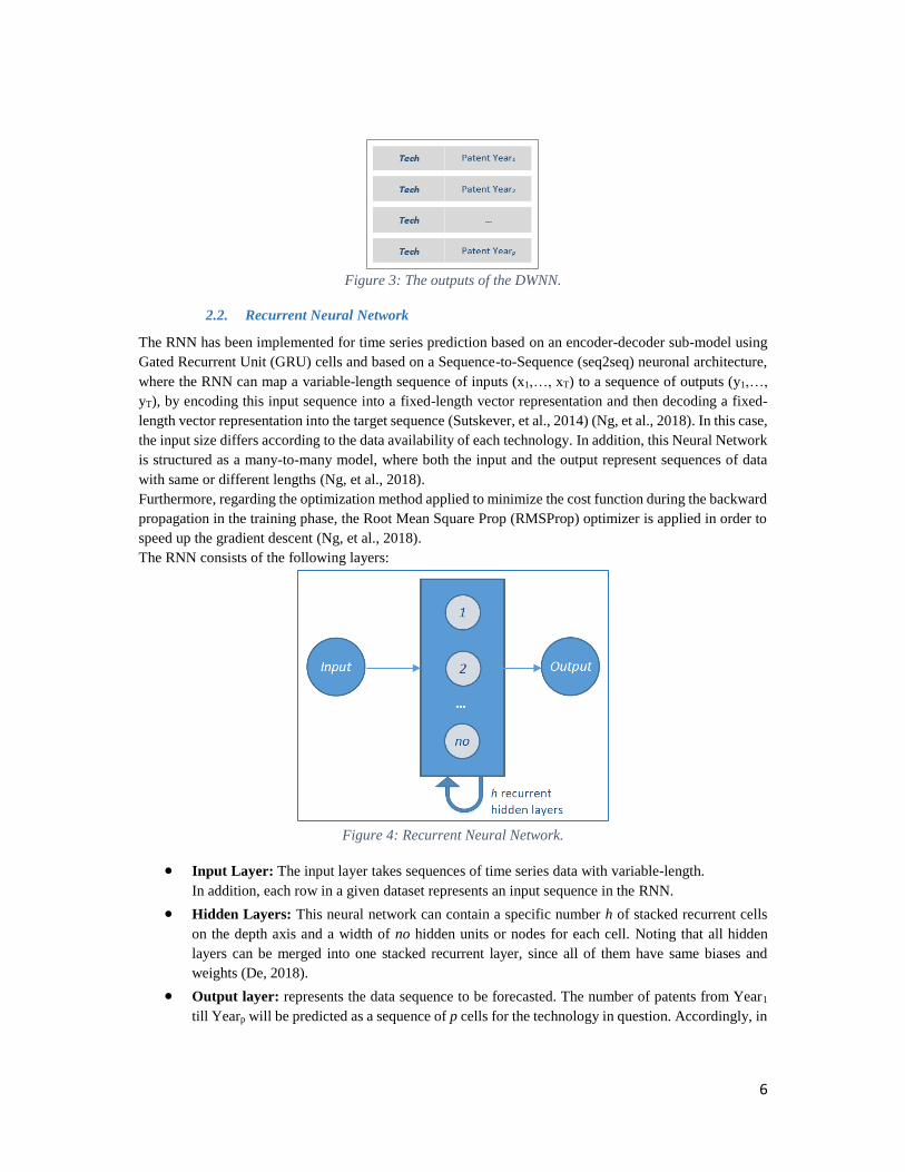
2.2. Recurrent Neural Network

The RNN has been implemented for time series prediction based on an encoder-decoder sub-model using

Gated Recurrent Unit (GRU) cells and based on a Sequence-to-Sequence (seq2seq) neuronal architecture,

where the RNN can map a variable-length sequence of inputs (x1,…, xT) to a sequence of outputs (y1,…,

yT), by encoding this input sequence into a fixed-length vector representation and then decoding a fixed-

length vector representation into the target sequence (Sutskever, et al., 2014) (Ng, et al., 2018). In this case,

the input size differs according to the data availability of each technology. In addition, this Neural Network

is structured as a many-to-many model, where both the input and the output represent sequences of data

with same or different lengths (Ng, et al., 2018).

Furthermore, regarding the optimization method applied to minimize the cost function during the backward

propagation in the training phase, the Root Mean Square Prop (RMSProp) optimizer is applied in order to

speed up the gradient descent (Ng, et al., 2018).

The RNN consists of the following layers:

Figure 4: Recurrent Neural Network.

Input Layer: The input layer takes sequences of time series data with variable-length.

In addition, each row in a given dataset represents an input sequence in the RNN.

Hidden Layers: This neural network can contain a specific number h of stacked recurrent cells

on the depth axis and a width of no hidden units or nodes for each cell. Noting that all hidden

layers can be merged into one stacked recurrent layer, since all of them have same biases and

weights (De, 2018).

Output layer: represents the data sequence to be forecasted. The number of patents from Year1

till Yearp will be predicted as a sequence of p cells for the technology in question. Accordingly, in

7

this case, Step 11 is not needed given that the prediction of the number of patents of all y years is

executed at a single step: that means y = p.

Figure 5: The output sequence of the RNN.

Experimentation

We collected patent data for 11 trending technologies over a period of time, in order to train and test the

neural network. The two Neural Networks models are applied on two candidate technologies to predict the

number of patents for the next five years: in this case the parameter p is equal to 5.

1. Data collection

1.1. Technologies listing

The selected technologies are listed based on several web sources, such as: IEEE (IEEE, 2016) (IEEE,

2015), Gartner (Cearley, et al., 2017), Elsevier (Peter Edelstein, 2017), Scientific American (Meyerson,

2015), MIT Technology Review (MIT Technology Review, 2018), etc. Therefore, their related keywords

are extracted manually using different references, such as “thesaurus” (Thesaurus, 2013), “TechTerms”

(Tech Terms, 2018), etc. and inserted in the integrated database.

1.2. Patent data Source

A CSV file containing the granted patents applications published until 2016 has been downloaded from the

USPTO website and imported into the ‘Patents’ table in the database.

Therefore, given that the patents data extracted from the USPTO are not grouped or categorized by

technology, a script has been developed under Python in order to extract the needed data by technology

from the ‘Patents’ table, based on technologies keywords matching. Specifically, patents were categorized

by technology based on the title of the patent application: the text analysis can be conducted by searching

each keyword or term of each technology in the title of all patents applications (Sunghae, 2011).

Finally, the number of patents were counted and grouped by year and by technology. The result was then

inserted into the ‘NumberOfPatents’ table.

The following figure represents the number of patents variation for a list of technologies:

Figure 6: Number of patents variation of different technologies from 1965 to 2016.

8

2. Training, Testing and Prediction datasets creation

The data in the ‘NumberOfPatents’ table have been split manually into training and validation datasets

based on the correlation between the number of patents of the technologies, since we have a limited amount

of data. The following figures illustrate samples of the original data:

Figure 7: A sample of the training data.

Figure 8: A sample of the testing data.

As per figure 6, 7 and 8, the number of patents of the “Autonomous Vehicles" technology in the testing

dataset is correlated with the "Big data and visualization" technology in the training dataset, since the

variation of their number of patents is approximately similar through the years. Moreover, the

“Cloud/Client computing" technology in the testing dataset is correlated as well with the "Augmented

Reality" technology that belongs to the training dataset.

Regarding the Prediction dataset, it contains the patent data related to the same technologies as the testing

dataset, in order to be able to compare the predicted values with the actual values, and therefore to visualize

the accuracy of the models. Accordingly, the prediction can be applied on any new technology using the

most accurate implemented model.

3. Neural Networks implementation

The implemented neural networks are based on different open source tutorials. The training parameters

have been tuned progressively, and the configurations in these experiments have been determined

experimentally based on the best obtained results, as suggested by Chevalier (Chevalier, 2018).

3.1. Wide and Deep Neural Network

In order to implement the WDNN, we have referred to the open source tutorial of TensorFlow under GitHub

(TensorFlow, 2017), with the following main parameters, as defined in the Proposed Methodology section:

a) Training

The training phase was processed by executing 10000 iterations, with a small learning rate equal to 0.001

in order to decrease the loss function and therefore to accelerate the training convergence (Ng, et al., 2018).

b) Validation and Prediction

In this section, the accuracy of this neural network was calculated as per the following steps and formulas:

p = 5 years; y = 1 year (as initial value); max = 45 years; n = 9; h = 5 hidden layers; no1 = 1000

nodes; no2 = 750 nodes; no3 = 500 nodes; no4 = 300 nodes; no5 = 150 nodes

9

i. First we normalized the expected and the predicted values on a scale from 0 to 100: the highest

value (max) in the expected values array was considered as 100, then the other expected (expected)

and predicted (pred) values was normalized accordingly:

ii. Then we calculated the absolute difference between the new normalized values of the expected

and the predicted arrays:

iii. Finally the accuracy was calculated by subtracting the average difference of the obtained values

from the total percentage:

3.2. Recurrent Neural Network

In order to implement the Sequence-to-Sequence neural network, we have referred to the open source code

of the “Signal prediction with a Sequence-to-Sequence Recurrent Neural Network model in TensorFlow”

(Chevalier, 2018), with the following main parameters, as defined in the Proposed Methodology section:

a) Training

The training phase was processed by executing 1000 iterations, with a small learning rate equal to 0.001 in

order to prevent divergent losses (Ravaut & Gorti, 2017) (Ng, et al., 2018).

b) Validation and Prediction

The accuracy of the RNN was calculated based on the same steps and formulas as for the WDNN.

4. Results

The graphs in the following subsections represent the obtained results for both candidate technologies in

the WDNN and the RNN, illustrating the quality of the prediction, where the abscissa axis represents the

time and the ordinate axis represents the number of patents.

As per the below results of the two neural networks, we note that the predicted numbers of patents for the

“Autonomous Vehicles" technology are following the same pattern as the "Big data and visualization"

technology, concluding that the correlation mentioned earlier between these two technologies was detected

by the neural networks during the prediction phase with a certain accuracy rate. The same applies to the

“Cloud/Client computing" and the "Augmented Reality" technologies.

4.1. Wide and Deep Neural Network

Table 2: Prediction accuracy for the WDNN.

Wide and Deep Neural Network

p = 5 years; max = 45 years; n = 5; h = 2 recurrent cells; no = 250 hidden units per cell

10

Figure 9: Actual and predicted number of patents in the WDNN for the "Cloud/Client computing"

technology from 1995 to 2016.

Figure 10: Actual and predicted number of patents in the WDNN for the "Autonomous Vehicles"

technology from 1991 to 2016.

4.2. Recurrent Neural Network

Table 3: Prediction accuracy for the RNN.

"Cloud/Client computing" (Figure 9) "Autonomous Vehicles" (Figure 10)

Actual or true

values

Predicted Values Actual or true values Predicted Values

114 126 96 53

180 113 61 43

173 154 28 32

169 222 10 22

98 265 5 22

Prediction accuracy: 64.66% Prediction accuracy: 80.41%

Average prediction accuracy: 72.53%

Recurrent Neural Network

"Cloud/Client computing" (Figure 11) "Autonomous Vehicles" (Figure 12)

Actual or true

values

Predicted Values Actual or true values Predicted Values

114 187 96 69

180 234 61 67

173 241 28 34

169 251 10 11

11

Figure 11: Actual and predicted number of patents in the RNN for the "Cloud/Client computing"

technology from 1995 to 2016.

Figure 12: Actual and predicted number of patents in the RNN for the "Autonomous Vehicles" technology

from 1991 to 2016.

Conclusion and discussion

The development of new and innovative technology-based products creates business value in today’s

economy, and therefore, forecasting technologies success becomes a crucial need. However, predicting

technologies success is a complex task in terms of prediction accuracy and data availability. Accordingly,

a novel method has been proposed in this paper, relying on patent analysis as a quantitative approach, and

using Neural Networks models in order to measure the candidate technologies power based on the

prediction of patents growth. Addressing this estimation is a necessary prerequisite before proceeding with

investments.

This method has been implemented using the USPTO Patent Database, with a comparative study of two

Neural Networks: a Wide and Deep Neural Network and a Recurrent Neural Network, and experimented

on 11 trending technologies to train and test these neural networks then applied on two candidate

technologies, "Cloud/Client computing” and “Autonomous Vehicles”, for the prediction phase.

The findings showed that RNN is more performing and accurate than WDNN.

Therefore, the proposed method answers questions related to technology success and appropriate prediction

models. Accordingly, it supports decision making of innovative technology-based product/service

development.

This study can be further enhanced by tackling its current limitations. The most challenging task faced in

our study is the access to accurate Big data, as the data are currently limited to a small dataset extracted

98 129 5 11

Prediction accuracy: 65.45% Prediction accuracy: 90.16%

Average prediction accuracy: 77.8%

12

only from the USPTO database and based uniquely on the granted patents applications, published until

2016. In addition, patent data are categorized by technology based on keywords matching of only the title

of the patent application. They can be queried as well in the application abstracts and other fields.

Furthermore, future works can further evolve the proposed research design to include additional factors or

dimensions affecting future technology success.

References

ALSHEIKH, M. A., LIN, S., NIYATO, D. & TAN, a. H.-P., 2014. Machine learning in wireless sensor

networks:Algorithms, strategies, and applications. IEEE Communications Surveys and Tutorials, Volume

16(4), pp. 1996-2018.

Altuntas, S., Dereli, T. & Kusiak, A., 2015. Forecasting technology success based on patent.

Technological Forecasting and Social Change, Volume 96, pp. 202-214.

Antonipillai, J., 2016. Intellectual Property and the U.S. Economy: 2016 Update. [Online]

Available at: https://www.uspto.gov/learning-and-resources/ip-motion/intellectual-property-and-us-

economy

Baller, S. et al., 2016. The Global Competitiveness Report 2016-2017, s.l.: World Economic Forum.

Banerjee, S., 2018. An Introduction to Recurrent Neural Networks. [Online]

Available at: https://medium.com/explore-artificial-intelligence/an-introduction-to-recurrent-neural-

networks-72c97bf0912

Bishop, C., 2006. Pattern Recognition and Machine Learning. 1 ed. New York: Springer.

Brownlee, J., 2017. How Does Attention Work in Encoder-Decoder Recurrent Neural Networks. [Online]

Available at: https://machinelearningmastery.com/how-does-attention-work-in-encoder-decoder-

recurrent-neural-networks/

Brownlee, J., 2017. Machine Learning Mastery. [Online]

Available at: https://machinelearningmastery.com/classification-versus-regression-in-machine-learning/

Brownlee, J., 2018. A Gentle Introduction to k-fold Cross-Validation. [Online]

Available at: https://machinelearningmastery.com/k-fold-cross-validation/

Cearley, D. W., Burke, B. & Samantha Searle, M. J. W., 2017. Top 10 Strategic Technology Trends for

2018. [Online]

Available at: https://www.gartner.com/doc/3811368?srcId=1-7251599992&cm_sp=swg-_-gi-_-dynamic

13

Cheng, H.-T., 2016. Wide & Deep Learning: Better Together with TensorFlow. [Online]

Available at: https://ai.googleblog.com/2016/06/wide-deep-learning-better-together-with.html

Cheng, H.-T.et al., 2016. Wide & Deep Learning for Recommender Systems, s.l.: Google.

Chen, H., Zhang, G., Zhu, D. & Lu, J., 2017. Topic-based technological forecasting based on patent data:

A case study of Australian patents from 2000 to 2014. Technological Forecasting and Social Change,

Volume 119, pp. 39-52.

Chevalier, G., 2018. seq2seq-signal-prediction. [Online]

Available at: https://github.com/guillaume-chevalier/seq2seq-signal-prediction

Cho, H. P. et al., 2018. Patent analysis for forecasting promising technology in high-rise building

construction. Technological Forecasting and Social Change, March, Volume 128, pp. 144-153.

Chung, J., Gulcehre, C., Cho, K. & Bengio, Y., 2014. Empirical Evaluation of Gated Recurrent Neural

Networks on Sequence Modeling. arXiv preprint arXiv:1412.3555.

Dean, J. et al., 2012. Large scale distributed deep networks. Advances in neural information processing

systems, pp. 1223-1231.

De, D., 2018. RNN or Recurrent Neural Network for Noobs. [Online]

Available at: https://hackernoon.com/rnn-or-recurrent-neural-network-for-noobs-a9afbb00e860

Dereli, T. & Kusiak, A., 2015. Forecasting technology success based on patent. Technological

Forecasting and Social Change, Volume 96, pp. 202-214.

Deshpande, A., 2016. A Beginner's Guide To Understanding Convolutional Neural Networks Part 2.

[Online]

Available at: https://adeshpande3.github.io/A-Beginner%27s-Guide-To-Understanding-Convolutional-

Neural-Networks-Part-2/

Duchi, J., Hazan, E. & Singer, Y., 2011. Adaptive Subgradient Methods for Online Learning. Journal of

Machine Learning Research, p. 12:2121–2159.

Elaraby, N., Elmogy, M. & Barakat, S., 2016. Deep Learning: Effective Tool for Big Data Analytics.

International Journal of Computer Science Engineering (IJCSE), Volume 5, pp. 254-262.

Foram Panchal, M. P., 2015. Optimizing Number of Hidden Nodes for Artificial Neural Network using

Competitive Learning Approach. International Journal of Computer Science and Mobile Computing, p.

358 – 364.

14

Geum, Y., Lee, S., Yoon, B. & Park, Y., 2013. Identifying and evaluating strategic partners for

collaborative R&D: Index-based approach using patents and publications. Technovation, pp. 211-224.

Hall, B. H., 2004. Patent Data as Indicators, Berkeley: OECD.

IEEE, 2015. TOP 10 COMMUNICATIONS TECHNOLOGY TRENDS IN 2015. [Online]

Available at: http://www.comsoc.org/ctn/ieee-comsoc-ctn-special-issue-ten-trends-tell-where-

communication-technologies-are-headed-2015

IEEE, 2016. Top 9 Computing Technology Trends for 2016. [Online]

Available at: https://www.scientificcomputing.com/news/2016/01/top-9-computing-technology-trends-

2016

Investopedia, 2018. Gross Domestic Product - GDP. [Online]

Available at: https://www.investopedia.com/terms/g/gdp.asp

Jneid, M. & Saleh, I., 2015. Improving start-ups competitiveness and innovation performance: the case of

Lebanon. s.l., The International Society for Professional Innovation Management (ISPIM).

Jo, K. G., Sung, P. S. & Sik, J. D., 2015. Technology Forecasting using Topic-Based Patent Analysis.

Journal of Scientific & Industrial Research, pp. 265-270.

Jun, S., Park, S. S. & Jang, D. S., 2012. Technology forecasting using matrix map and patent clustering.

Industrial Management and Data Systems, Volume 112(5), pp. 786-807.

Kim, J. & Lee, S., 2017. Forecasting and identifying multi-technology convergence based on patent data:

the case of IT and BT industries in 2020. S. Scientometrics, Volume 111, pp. 47-65.

Lee, C., Kwon, O., Kim, M. & Kwon, D., 2017. Early identification of emerging technologies: A machine

learning approach using multiple patent indicators. Technological Forecasting & Social Change, Volume

127, pp. 291-303.

Meyerson, B., 2015. Top 10 Emerging Technologies of 2015. [Online]

Available at: https://www.scientificamerican.com/article/top-10-emerging-technologies-of-20151/

MIT Technology Review, 2018. 10 Breakthrough Technologies 2015. [Online]

Available at: https://www.technologyreview.com/lists/technologies/2015/

Najafabadi, M. et al., 2015. Deep Learning applications and challenges in Big Data analytics. Journal of

Big Data, Volume 2(1), p. 1.

15

National Science Board, 2014. Science and Engineering Indicators, s.l.: National Science Foundation.

Ng, A., Katanforoosh, K. & Mourri, Y. B., 2018. Different types of RNNs. [Online]

Available at: https://www.coursera.org/lecture/nlp-sequence-models/different-types-of-rnns-BO8PS

Ng, A., Katanforoosh, K. & Mourri, Y. B., 2018. Learning rate decay. [Online]

Available at: https://www.coursera.org/lecture/deep-neural-network/learning-rate-decay-hjgIA

Ng, A., Katanforoosh, K. & Mourri, Y. B., 2018. Recurrent Neural Network Model. [Online]

Available at: https://www.coursera.org/lecture/nlp-sequence-models/recurrent-neural-network-model-

ftkzt

Ng, A., Katanforoosh, K. & Mourri, Y. B., 2018. RMSprop. [Online]

Available at: https://www.coursera.org/lecture/deep-neural-network/rmsprop-BhJlm

OECD, 2009. Innovation and Growth: Chasing a Moving Frontier. Paris: OECD.

Peter Edelstein, M., 2017. Top trends in health information & communications technology for 2017.

[Online]

Available at: https://www.elsevier.com/connect/top-trends-in-health-information-and-communications-

technology-for-2017

Prabhu, 2018. Understanding of Convolutional Neural Network (CNN) — Deep Learning. [Online]

Available at: https://medium.com/@RaghavPrabhu/understanding-of-convolutional-neural-network-cnn-

deep-learning-99760835f148

Ravaut, M. & Gorti, S. K., 2017. Faster gradient descent via an adaptive learning rate, Toronto: s.n.

Rizwan, M., 2018. RMSProp. [Online]

Available at:

https://engmrk.com/rmsprop/?utm_campaign=News&utm_medium=Community&utm_source=DataCam

p.com

Ruder, S., 2016. An overview of gradient descent optimization algorithms, s.l.: arXiv preprint

arXiv:1609.04747.

Sapna, S., 2016. Fusion of big data and neural networks for predicting thyroid. Mysuru, IEEE, pp. 243-

247.

Saunders, A. A., 2017. Top 5 Use Cases of TensorFlow. [Online]

Available at: https://www.digitaldoughnut.com/articles/2017/march/top-5-use-cases-of-tensorflow

16

Schmidhuber, J., 2015. Deep Learning in Neural Networks: An Overview. Neural Networks, Volume 61,

pp. 85-117.

Scikit Learn, 2018. sklearn.model_selection.KFold. [Online]

Available at: http://scikit-learn.org/stable/modules/generated/sklearn.model_selection.KFold.html

Shanmuganathan, S. & Samarasinghe, S., 2016. Artificial Neural Network Modelling. s.l.:Springer

International Publishing.

Sunghae, J., 2011. IPC Code Analysis of Patent Documents Using Association Rules and Maps – Patent

Analysis of Database Technology. Berlin, Heidelberg, Springer, pp. 21-30.

Surmenok, P., 2017. Estimating an Optimal Learning Rate For a Deep Neural Network. [Online]

Available at: https://towardsdatascience.com/estimating-optimal-learning-rate-for-a-deep-neural-network-

ce32f2556ce0

Sutskever, I., Vinyals, O. & Le, Q. V., 2014. Sequence to Sequence Learning with Neural Networks. s.l.,

Google, pp. 3104-3112.

Tech Terms, 2018. The Tech Terms Computer Dictionary. [Online]

Available at: https://techterms.com

TensorFlow, 2017. wide_n_deep_tutorial. [Online]

Available at: https://github.com/baidu-research/tensorflow-

allreduce/blob/master/tensorflow/examples/learn/wide_n_deep_tutorial.py

TensorFlow, 2018. About TensorFlow. [Online]

Available at: https://www.tensorflow.org/

TensorFlow, 2018. DNNLinearCombinedRegressor. [Online]

Available at:

https://www.tensorflow.org/api_docs/python/tf/contrib/learn/DNNLinearCombinedRegressor

TensorFlow, 2018. Linear Combined Deep Neural Networks. [Online]

Available at: https://tensorflow.rstudio.com/tfestimators/reference/dnn_linear_combined_estimators.html

Thesaurus, 2013. thesaurus. [Online]

Available at: http://www.thesaurus.com

17

Thrideep, S. K., 2017. Artificial Neural Networks - The Future of Airline Sales and Revenue forecasting.

[Online]

Available at: https://www.linkedin.com/pulse/artificial-neural-networks-future-airline-sales-krishnan-

thrideep?trk=portfolio_article-card_title

USPTO, 2018. USPTO. [Online]

Available at: https://www.uspto.gov/

WILDML, 2018. DEEP LEARNING GLOSSARY. [Online]

Available at: http://www.wildml.com/deep-learning-glossary/#rmsprop

Wu, F.-S., Lee, P.-C., Shiu, C.-C. & Su, H.-n., 2010. Integrated methodologies for mapping and

forecasting science and technology trends: A case of etching technology. Phuket, Thailand, IEEE, pp.

2159-5100.