Truax

1

Predicting Initial Production ofGranite Wash Horizontal Wells Using Old Well Logs and Cores

13 November 2014

Granite Wash Workshop

Authors: Narayan Nair, Matt Padgham, Jerome Truax

0

1000

2000

3000

4000

0.01 0.1 1

Oil In

itia

l P

rod

ucti

on

, S

TB

/D

Production Indicator from vertical logs

Strong correlation, eh?

Truax

2

Method and Outline for Talk• Determine production contribution log (IP FOM)

– Based on volumetrics and permeability

– Petrophysics and Log Analysis Steps

• Sum over a reservoir interval and upscale to reservoir-scale permeability derived from well production data (PI parameter)

• Use PI to predict initial production of potential horizontal wells– Generate maps of PI parameter

– Compare to production data

Note: more slides are included here than will be covered in the talk.

Twelve-Step Granite Wash Log Analysis

4

Groundwork1. Geology discussions2. Core & cuttings study3. Log triage and repair4. GR & neutron environmental corrections5. Facies analysis

Calculations6. VShale7. Total & effective porosity8. Saturation9. Permeability & production10. Flagging11. Summations12. Fraccability

Truax

3

1a

1b

Truax

4

1c

1d) Tx panhandle granite wash characteristics

• Source material is mostly uplifted Paleozoic sediments & carbonate, plus Precambrian granite, diabase, and granodiorite. There are a few thin beds of limestone and shale interspersed. Composition varies widely.

• The depositional environment is primarily stacked deltas, river channels, and turbidites. Paleoslopes range from steep to quiescent. There are many beds that contain re-worked material.

• Feldspar content, grain size, and alteration vary widely and wildly, vertically and areally. Chorite is ubiquitous.

• Reservoirs are often separated by 10-30 ft thick marine and terrestrial shales and flooding deposits.

Truax

5

1e) Tx panhandle granite wash exploitation

• There are about 100,000 vertical wells through the granite wash; many reach below to the Morrow and other horizons.

• Perms of present-day reservoirs are typically near 500 nd.

• Two or three 5000-ft laterals are typically drilled per section in one horizon. There are often stacked laterals.

• Slickwater fracs appear to be the most effective.

• Fraccing severely “bashes” adjacent producing wells where pressures have been lowered.

• Prospecting is done by sifting through production data and old logs.

• Recently there has been some drilling of “pilot” holes, or vertical holes before the turn, with coring and logging.

1g) box 12

Truax

6

1f) box 11

1h) box 10

Truax

7

1i) core and hi-res log

13

2a) Core permeability vs porosity

14

Slope: 3 p.u. per log cycle

Intercept:Tuning Parameter

Slope:5 p.u. per log cycle

y = 0.0001e51.4x

R² = 0.96

0.0001

0.0010

0.0100

0.1000

0.0000 0.0200 0.0400 0.0600 0.0800 0.1000

Co

re p

erm

(m

d)

Core PorosityKlinkenberg

Truax

8

2b) More core permeability

15

2c) What is core porosity?

Th

K

Truax

9

17

2d) What is core porosity?

RHOBNPHITPOREPOR

2e) Volume fractions of a formation

Hydrocarbons - VhcEffective water - VweShale - Vsh

Effective porosity - fe

Total porosity - ft

Total water - Vwt

Matrix

Vmatrix

Dry Clays & Silt

Vdcs

Clay-bound water

Vwb

Capillary-bound waterVcap

Free water

Vwf

Oil

Voil

Gas

Vgas

Wet Solids – Vwetsolids or 1- fe

1- Vsh - fe

Dry Solids Vdrysolids or 1- ft

Total irreducible water - BVIW

Swt = Vwt / ft

Swe = Vwe / fe

Free Fluid – FFI or ff

Truax

10

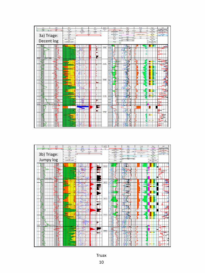
3a) Triage: Decent log

3b) Triage: Jumpy log

Truax

11

Proximal Distal

4e) Log Facies based on six wells

• Use Buckles plot to assess irreducible water for log facies

• Include results in Tixier or Coates perm calculations

Twelve-Step Granite Wash Log Analysis

22

Groundwork1. Geology discussions2. Core & cuttings study3. Log triage and repair4. GR & neutron environmental corrections5. Facies analysis

Calculations6. VShale7. Total & effective porosity8. Saturation9. Permeability & production10. Flagging11. Summations12. Fraccability

Truax

12

9) Definitions

Indicator i r hPI h k Sf

Log curve

Indicator i r hPI h k SfIP FOM =

Log summation across interval

24

Example 1a

Truax

13

25

Example 1b

Example 2

Th

K

Truax

14

Example 3

Example 4(sorry about thepoor resolution)

Truax

15

Reservoir Accounting1. The initial production rates of a horizontal well in linear flow will be

driven primarily by a lumped parameter Jlt, which is dependent on both

rock quality (perm – k) and stimulation effectiveness (total frac surface

area Af), and pressure drawdown imposed on the well.

2. For comparing wells of similar initial reservoir pressures we can skip

normalizing the initial formation volume factor Bi, initial viscosity μi, and

approximate initial total compressibility cti using hydrocarbon saturation

Sh. The permeability kr is effective to primary hydrocarbon phase.

3. The flow rate of each flow unit (i) will be proportional to the net pay h,

the fracture half-length propagated in each unit xf, and its flow capacity.

Fracture design related variations in xf can be modeled as needed, for simplicity assume rectangular geometry – equal in all units.

4. Early life total flow rate in in tight reservoirs is the sum of the individual flow units; ignore crossflow. The total well rate is the sum of the net pay and flow capacity of each flow unit. For simplicity, the flow units can be the log sampling interval ½ feet intervals.

5. The productivity index indicator is defined and in LINE’s experience is correlated to well performance; and can be used as a rock quality index.

6. The upscaled* values of permeability can be calculated from the PI indicator for the tuning to well production results.

Review SPE 139097, 166468, and 166468 for theory and methods to normalize pressure drawdown, and completion practices.29

IP ltQ J P

1lt f r ti

i i

J A k cB

f

i fi i r hq x h k Sf

T i r hq h k Sf

Indicator i r hPI h k Sf

2

*

* *

1 indicator

h

PIk

S hf

2

1

3

4

5

6

SPE 139097, 162843, 166468

Lookback – Hz. Kansas City Oil Program

• The Kansas City is a matrix-flow dominated prolific reservoir in the Granite Wash play in Wheeler TX.

• Identical completion practices and pressure drawdown was used in Linn operated wells.

• Clear correlation between highest oil production rates seen in these hz. wells compared to log-calculated productivity index.30

0

1000

2000

3000

4000

0.01 0.1 1

Oil I

P,

ST

B/D

P.I. Indicator

Truax

16

IP and Net Pay comparison

31

Net Pay Isopach

IP map

y = 19455xR² = 0.8579

0

2,000

4,000

6,000

8,000

10,000

12,000

14,000

0.0 0.1 0.2 0.3 0.4 0.5 0.6 0.7 0.8 0.9 1.0

Gas

IP (

Mcf

/d)

Productivity Indicator= Net Pay * Sqrt(Epor x K* x Shc)

Existing Wells Productivity Estimate Linear (Existing Wells)

Dyco Granite Wash ‘A’ ExampleIP vs. Productivity Indicator

Initial correlation based on 3 wells with data.

LOG BASED PRODUCTIVITY32

Truax

17

y = 36.612xR² = 0.7634

y = 19.429xR² = 0.398

0

5

10

15

20

25

30

0.0 0.1 0.2 0.3 0.4 0.5 0.6 0.7 0.8 0.9 1.0

Af*

Sqrt

(k)/

Mp

Productivity Indicator= Net Pay * Sqrt(Epor x K* x Shc)

Single Wells Increased Density Wells Linear (Single Wells) Linear (Increased Density Wells)

Dyco Granite Wash ‘A’ ExampleLog Estimated vs. Actual Productivity

WEL

L P

RO

DU

CTI

VIT

Y /

LB

PR

OP

PAN

T

LOG BASED PRODUCTIVITY

“Single” wells exhibit increased productivity that

suggests significant contribution from natural

fractures.

33

Dyco Granite Wash ‘B’Permeability Upscaling

0.000000

0.000200

0.000400

0.000600

0.000800

0.001000

0.000000 0.000200 0.000400 0.000600 0.000800 0.001000

Up

scal

edP

erm

eab

ility

fro

m 3

PU

/Dec

ade

Tra

nsf

orm

(mD

)

Permeability From Rate Transient Analysis (mD)

Most likely perms based

on 75% cluster

efficiency

𝑈𝑝𝑠𝑐𝑎𝑙𝑒𝑑 𝑃𝑒𝑟𝑚 = 10(33.3∗𝑃𝑜𝑟𝑜𝑠𝑖𝑡𝑦𝐸𝑓𝑓𝑒𝑐𝑡𝑖𝑣𝑒 −5.6)

Perm range of 200-600 nD observed

Truax

18

Dyco Granite Wash ‘B’PI Indicator vs. Peak Rate

35

y = 13749xR² = 0.5402

0

2000

4000

6000

8000

10000

12000

14000

16000

0 0.2 0.4 0.6 0.8 1

30

Day

Pe

ak G

as R

ate

(M

cfp

d)

Productivity Index= Net Pay x Sqrt(Epor x k* x SHC)

PI Indicator vs. Peak Gas Rate (Mcfpd)

Peak 30 Day Rate (Mcfpd) Linear (Peak 30 Day Rate (Mcfpd))

2009 Completion2nd or 3rd Well in SectionDamage (Low FCD)

Dyco Britt PI Indicator

36

0

2

4

6

8

10

12

14

16

0.2 0.4 0.6 0.8 1.0 1.2 1.4 1.6 1.8

2 St

ream

IP (

MM

CFE

/D)

PI Indicator (scaled)

2 Stream IP vs PI Indicator - Britt

First Wells

Second Wells

Linear (First Wells)

Truax

19

Stiles Ranch GWB Productivity Estimate- IP Indicator

37

y = 0.97xR² = 0.6166

0

1000

2000

3000

4000

5000

6000

7000

0 1000 2000 3000 4000 5000 6000 7000

30 D

ay IP

Rat

e (M

cfp

d)

Log Based IP Prediction (Mcfpd)

STILES RANCH GWB

PRODUCERS Linear (PRODUCERS)

Conclusions

• Maps based on PI can be used as supplements to more traditional net pay maps.

• PI is a valuable predictor of performance of proposed wells.

• This concept has been used over the past few years to improve bottom line success.