Important Notice

This copy may be used only for the purposes of research and

private study, and any use of the copy for a purpose other than research or private study may require the authorization of the copyright owner of the work in

question. Responsibility regarding questions of copyright that may arise in the use of this copy is

assumed by the recipient.

UNIVERSITY OF CALGARY

Predicting heavy oil and bitumen viscosity from well logs and calculated seismic properties

by

Eric Anthony Rops

A THESIS

SUBMITTED TO THE FACULTY OF GRADUATE STUDIES

IN PARTIAL FULFILMENT OF THE REQUIREMENTS FOR THE

DEGREE OF MASTER OF SCIENCE

GRADUATE PROGRAM IN GEOLOGY AND GEOPHYSICS

CALGARY, ALBERTA

APRIL, 2017

© Eric Anthony Rops 2017

ii

Abstract

Viscosity is the most important parameter influencing heavy oil production and

development. While heavy oil viscosities can be measured in the lab from core and wellhead

samples, it would be very useful to have a method to reliably estimate heavy oil viscosity

directly from well logs.

Multi-attribute analysis enables a target attribute (viscosity) to be predicted from other

known attributes (the well logs). The viscosity measurements were generously provided by

Donor Company, which allowed viscosity prediction equations to be trained.

Once the best method of training the prediction was determined, viscosity was

successfully predicted from resistivity, gamma-ray, NMR porosity, spontaneous potential, and

the sonic logs. The predictions modelled vertical viscosity variations throughout the reservoir

interval, while matching the true measurements with a 0.76 correlation.

Another set of viscosity predictions were generated using log-derived seismic properties.

The top viscosity-predicting seismic properties were found to be P-wave velocity and acoustic

impedance. They predicted viscosity with an average validation error less than one standard

deviation, however the predictions were less detailed with a correlation of only 0.35.

Also explored in this thesis was the effect of including depth as a viscosity predictor,

predicting viscosity from acoustic logs scaled to seismic frequencies, and bitumen-water contact

detection from acoustic logs.

iii

Acknowledgements

First and foremost, I want to thank my supervisor, Dr. Larry Lines, for taking me on as

his (potentially last) student. I am grateful to him for giving me the freedom to pursue a topic of

great interest to me, and for his constant encouragement and positivity. This thesis was an

interesting progression stemming from my GOPH 701 work in April 2015 and has evolved ever

since.

A special thank-you to Bob Everett who took an interest to this research at

GeoConvention 2016. Since then he has consistently offered his professional advice assisting me

with the well log analysis, and even gave me a two-week crash course in advanced petrophysical

interpretation. I cannot state enough how valuable that was for me.

I also want to thank David Gray, Scott Keating, Doug Clark, Rudy Strobl, Kevin Pyke,

and Xianfeng Zhang for their thoughts and suggestions related to this work. This thesis could not

have turned out as it did without the contributions from all these individuals.

A sincere thank-you to Dr. Brian Russell and Dr. Brij Maini for taking the time to be on

my defense committee and for actually having to read this whole thesis. Thank-you also to Dr.

Roy Lindseth for graciously assisting with the technical writing.

Thank-you to CREWES sponsors and NSERC for funding this research, to the

anonymous donor company for providing the viscosity data, and to CGG Hampson-Russell for

making their software available to CREWES students.

Finally, I want to acknowledge Bobby Gunning, Jason Levesque, Adriana Gordon,

Andrew Mills, and several others for helping make my graduate student experience as enjoyable

as it was!

iv

Table of Contents

Abstract .............................................................................................................................. ii

Acknowledgements .......................................................................................................... iii Table of Contents ............................................................................................................. iv List of Tables .................................................................................................................... vi List of Figures and Illustrations .................................................................................... vii List of Symbols, Abbreviations and Nomenclature ...................................................... xi

Chapter 1 – Introduction ..................................................................................................1 1.1 - Introduction to oil sands, heavy oil, and viscosity ..............................................1 1.2 – Shear properties of heavy oil ...............................................................................5

1.3 – Previous studies of estimating heavy oil viscosity ..............................................9 1.4 – Motivation and goals of this thesis ....................................................................11

Chapter 2 – Well Logging Principles .............................................................................13

2.1 – Overview of the well log measurement .............................................................13 2.2 – Overview of the total gamma ray tool ...............................................................14

2.3 – Overview of the induction resistivity tool .........................................................15 2.4 – Overview of the spontaneous potential (SP) tool .............................................17 2.5 – Overview of the density logging tool .................................................................19

2.6 – Overview of the sonic logging tool .....................................................................21 2.7 – Overview of Nuclear Magnetic Resonance (NMR) logging ............................25

Chapter 3 – Theory of Multilinear Regression .............................................................29

3.1 – Multi-Attribute Analysis ....................................................................................29

3.2 – Step-Wise Regression .........................................................................................32 3.3 – Cross-Validation .................................................................................................33

Chapter 4 – Study Area Geology and Dataset...............................................................36

4.1 – Introduction to Study Area ................................................................................36 4.2 – Study Area Geology ............................................................................................37

4.3 – Dataset ..................................................................................................................42

Chapter 5 – Problem Setup, and Viscosity Prediction Results ....................................45 5.1 – Well log normalization process ..........................................................................45

5.2 – Adding NMR logs as viscosity predicting attributes .......................................47

5.3 – Viscosity training model .....................................................................................49 5.4 – Viscosity prediction results from all logs, and seismic properties ..................51 5.5 – Visualizing the viscosity predictions .................................................................54

5.6 – Viscosity prediction from standard logs, and predicting log10(viscosity) .....61 5.7 – Blind test on a well from a nearby reservoir ....................................................65 5.8 – Adding depth as a viscosity predictor ...............................................................67 5.9 – Predicting viscosity using acoustic logs upscaled to seismic frequencies .......71 5.10 – Predicting resistivity from log-derived seismic properties ...........................74

v

Chapter 6 – Discussion and Conclusions .......................................................................78 6.1 – Comments regarding the well logs used to predict viscosity ..........................78 6.2 – Concluding remarks regarding viscosity prediction from all well logs .........80

6.3 – Concluding remarks regarding viscosity prediction from standard well

logs only.................................................................................................................81 6.4 – Concluding remarks regarding viscosity prediction from calculated

seismic properties .................................................................................................81 6.5 – Concluding remarks regarding depth as a viscosity predictor .......................82

6.6 – Concluding remarks regarding the potential of seismic data for viscosity

prediction ..............................................................................................................82 6.7 – Future Work ........................................................................................................83 6.8 – Final Remark .......................................................................................................84

References .........................................................................................................................86

Appendices ........................................................................................................................90

A.1. Viscosity prediction equations ............................................................................90 A.2. Other useful prediction equations not discussed in the main text ...................92

A.3. Viscosity - Depth relation from the ConocoPhillips Surmont project ............93

vi

List of Tables

Table 5-1: Emerge™ top predicting attributes for NMR Total Porosity. ..................................... 47

Table 5-2: Emerge™ top predicting attributes for NMR Free Porosity. ...................................... 47

Table 5-3: Emerge™ top predicting attributes for NMR Moveable Fluid Porosity. .................... 47

Table 5-4: Comparison of the three viscosity prediction methods ............................................... 64

Table 5-5: Emerge™ top viscosity predicting attributes using acoustic logs upscaled to ................

seismic frequencies ....................................................................................................................... 71

Table 5-6: Emerge™ top resistivity predicting attributes from calculated seismic properties. .... 75

vii

List of Figures and Illustrations

Figure 1-1: Oil grade categories, defined by their API gravity values. .......................................... 1

Figure 1-2: Viscosity concept from laminar shear of two plates………………………………….2

Figure 1-3: Oil viscosities by grade category, compared to typical kitchen items. ........................ 3

Figure 1-4: Temperature dependence of oil viscosity using the Beggs & Robinson (1975)

relation at API values of -5, 10, and 25 .................................................................................. 4

Figure 1-5: Ultrasonic compressional waveforms measured through a very heavy oil (API = -

5) at -12.5oC and 49.3oC. ........................................................................................................ 5

Figure 1-6: Bulk modulus and shear modulus for an API 8o heavy oil .......................................... 6

Figure 1-7: Frequency dependence of velocity for a heavy oil saturated carbonate rock from

Texas. ...................................................................................................................................... 6

Figure 1-8: Shear modulus – temperature – frequency relation from lab measurements of a

heavy oil saturated carbonate from Uvalde, Texas ................................................................. 8

Figure 1-9: Viscosity tomogram from Vasheghani & Lines (2012). .............................................. 9

Figure 1-10: A pseudo-viscosity log produced from two NMR logging parameters (T2 and

HI), calibrated to laboratory viscosity measurements from the Athabasca oil sands ........... 11

Figure 2-1: The elements of well logging ..................................................................................... 13

Figure 2-2: The life of a single gamma ray, which is emitted in the formation and ultimately

detected by a NaI detector in the borehole ............................................................................ 15

Figure 2-3: The principle of the induction tool. ............................................................................ 16

Figure 2-4: Borehole mud invasion profile: “step model” of invasion ......................................... 17

Figure 2-5: A schematic representation of the development of the spontaneous potential

signal in a borehole ............................................................................................................... 18

Figure 2-6: Schematic diagram of a density tool .......................................................................... 19

Figure 2-7: A typical acoustic waveform recorded in a borehole ................................................. 22

Figure 2-8: Simplified schematic of a sonic array logging system.. ............................................. 23

Figure 2-9: a) An array of waveforms showing increasing moveout from near to far receivers.

b) A slowness-time map in which coherent peaks correlate to different wave

components. c) A continuous log is built from repeating steps (a) and (b) at each depth

measurement point ................................................................................................................ 24

viii

Figure 2-10: A summary of the idealized interpretation of T2 distributions for water wet

clastic rocks ........................................................................................................................... 26

Figure 2-11: NMR T2 distributions as a function of depth ........................................................... 27

Figure 2-12: Oil sands well in the study area with NMR data ...................................................... 28

Figure 3-1: (Left): Cross-plotting against 1 attribute gives a line best fit. (Right): Cross-

plotting against 2 attributes gives a planar best fit. ............................................................... 29

Figure 3-2: Illustration of the basic multi-attribute regression problem ....................................... 29

Figure 3-3: Example: Cross-plot of predicted Vp against measured Vp ...................................... 31

Figure 3-4: An Emerge™ prediction error plot. ........................................................................... 34

Figure 3-5: Illustration of how a higher order polynomial can over-fit the training data ............. 35

Figure 4-1: Distribution of Alberta’s oil sands deposits ............................................................... 36

Figure 4-2: Stratigraphic chart for the McMurray oil sands system ............................................. 38

Figure 4-3: Log suite for an example well in the study area ........................................................ 39

Figure 4-4: Stratigraphic framework for the McMurray Formation ............................................. 41

Figure 4-5: Map of the oil sands study area. ................................................................................. 43

Figure 4-6: Histogram of all laboratory viscosity measurements throughout the study area. ...... 44

Figure 4-7: Distribution map of the base reservoir viscosity measurements ................................ 44

Figure 5-1: Distribution of the gamma ray values for the 40 training wells................................. 45

Figure 5-2: What the normalized logs look like (red) versus the un-normalized logs (blue). ...... 46

Figure 5-3: Distribution of the 25 NMR wells in the study area .................................................. 48

Figure 5-4: Predicting NMR porosities from Resistivity, P-wave sonic, Gamma Ray, and

Neutron Porosity. Validation results for two example wells are shown. .............................. 49

Figure 5-5: Illustrating the old and new viscosity training models using all well logs ................ 50

Figure 5-6: Viscosity training model using only log-derived seismic properties ......................... 51

Figure 5-7: Top: Emerge™ prediction error plot and cross-plot for viscosity using the new

training model, and all the available well logs as the predicting attributes. In the

crossplot, each color represents a different well. Bottom: The list of attributes with their

associated validation errors. .................................................................................................. 52

ix

Figure 5-8: Top: Emerge™ prediction error plot and cross-plot for viscosity using the new

training model, and calculated seismic properties as the predicting attributes. In the

cross-plot, each color represents a different well. Bottom: The list of attributes with their

associated validation errors. .................................................................................................. 53

Figure 5-9: Viscosity predictions (validation results) for an example well where the viscosity

trend continues 20m above the top measurement. ................................................................ 56

Figure 5-10: Viscosity predictions (validation results) for an example well where two

viscosity gradients are modelled from 440m to 460m, separated by a shaley zone. ............ 57

Figure 5-11: Viscosity predictions (validation results) for an example well where two

viscosity gradients are modelled throughout the reservoir interval. ..................................... 58

Figure 5-12: Viscosity predictions (validation results) for an example well with a smooth

increasing viscosity gradient with depth, and a beautiful inverse correlation with

resistivity. .............................................................................................................................. 59

Figure 5-13: Viscosity measurements at 20oC and API gravity measurements plotted versus

depth for two wells in a nearby bitumen reservoir................................................................ 60

Figure 5-14: Top: Emerge™ prediction error plot and cross-plot for viscosity using the new

training model, and only the standard logs as predicting attributes. In the crossplot, each

color represents a different well. Bottom: The list of attributes with their associated

validation errors. ................................................................................................................... 62

Figure 5-15: Comparison of the three viscosity prediction methods for an example well ........... 63

Figure 5-16: Comparison of the three viscosity prediction methods for an example well. .......... 63

Figure 5-17: Location of the blind test well (yellow star) relative to the study area wells .......... 65

Figure 5-18: Prediction results in the blind test well 10km north of the study area ..................... 66

Figure 5-19: Viscosity measurements from all 40 training wells plotted against depth. .............. 67

Figure 5-20: Top: Emerge™ viscosity prediction error plot and cross-plot, using all well logs

plus depth as predicting attributes. For the cross-plot, each color represents a different

well. Bottom: The list of attributes with their associated validation errors .......................... 68

Figure 5-21: Top: Emerge™ viscosity prediction error plot and cross-plot, using log-derived

seismic properties plus depth as predicting attributes. For the cross-plot, each color

represents a different well. Bottom: The list of attributes with their associated validation

errors. .................................................................................................................................... 69

Figure 5-22: Influence of depth as a viscosity predictor for three example wells ........................ 70

x

Figure 5-23: Predicting viscosity from upscaled acoustic logs for a well with a continuous

20m reservoir interval. .......................................................................................................... 72

Figure 5-24: Predicting viscosity from upscaled acoustic logs for a well with several

interbedded shale intervals. ................................................................................................... 73

Figure 5-25: Resistivity prediction from log-derived seismic properties for three example

wells. ..................................................................................................................................... 76

Figure 5-26: Histogram of all bitumen density measurements throughout the study area. .......... 77

Figure A3-1: Viscosity measurements plotted against reservoir depth for the ConocoPhillips

Surmont oil sands project ...................................................................................................... 93

xi

List of Symbols, Abbreviations and Nomenclature

Symbol Definition

API

cP

DT

DTS

GR

GR-API

API gravity, ratio of the fluid density of oil to pure

water. Used for classifying oil grade.

Centipoise. Unit of viscosity measurement.

1 cP = 1 mPa*s = 0.001 Pa*s

Water = 1cP. Bitumen = millions of cP.

Compressional sonic log. Measures P-wave

slowness

Shear sonic log. Measures S-wave slowness

Gamma-ray log. Measures formation radioactivity

Unit of measurement for the gamma ray log

NMR

RHOB

SAGD

SP

Vp

Vs

Nuclear Magnetic Resonance logging. Responds

to hydrogen protons in formation

Formation bulk density log

Steam-assisted gravity drainage

Spontaneous potential log. Responds to electric

potential differences across rock boundaries

P-wave velocity

S-wave velocity

1

Chapter 1 – Introduction

1.1 - Introduction to oil sands, heavy oil, and viscosity

Oil sands consist of unconsolidated sand that is held together by bitumen (soluble organic

matter). World resources of bitumen and heavy oil are estimated to be 5.6 trillion barrels (20% to

25% of which are recoverable), compared with the remaining conventional crude oil reserves of

1.02 trillion barrels (Hein, 2006). Of the heavy oil and bitumen resources, over 80% are in

Venezuela, Canada and the U.S.A. The largest oil-sands deposits are in Alberta, Canada, which

account for more than 70% of world’s bitumen in place (Hein, 2006). In 2001, raw bitumen

production in Alberta surpassed conventional crude production for the first time, and in 2014,

total oil sands production from Alberta reached 2.3 million barrels per day (Teare et. al., 2014).

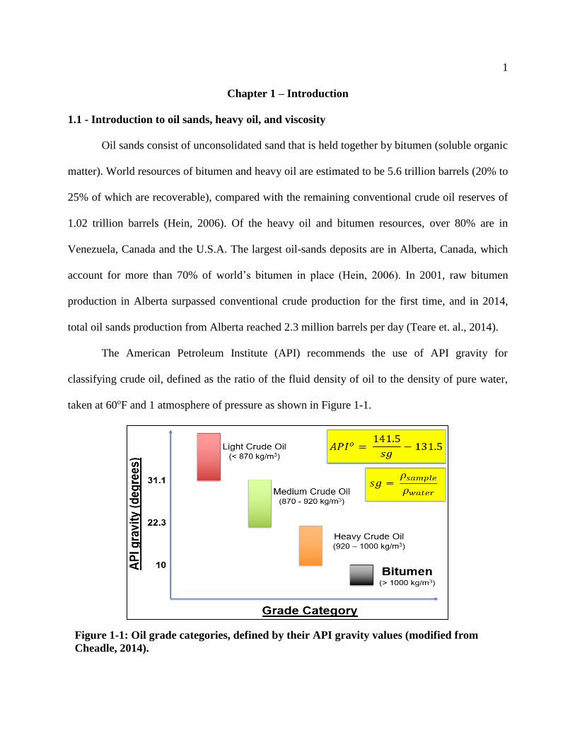
The American Petroleum Institute (API) recommends the use of API gravity for

classifying crude oil, defined as the ratio of the fluid density of oil to the density of pure water,

taken at 60oF and 1 atmosphere of pressure as shown in Figure 1-1.

Figure 1-1: Oil grade categories, defined by their API gravity values (modified from

Cheadle, 2014).

2

Heavy oil is defined as having 22.3°API gravity or less. Hydrocarbons of 10°API

(density of water) or less are defined as bitumen. In comparison, conventional crude oils have

densities greater than 22.3° API (Chopra et. al., 2010).

The fluid property that most greatly affects productivity and recovery is viscosity (Batzle

et. al., 2006). The more viscous the oil, more energy needs to be injected into the system to

reduce the viscosity to allow it to flow (ie. steam-assisted gravity drainage, or cyclic steam

stimulation).

Viscosity is a fluid’s resistance to deformation by shear stress, or more simply, a fluid’s

resistance to flow (McKennell, 1956). The definition of viscosity is given by Equation 1.1 and

illustrated in Figure 1-2 as laminar shear of fluid between two plates. From the diagram,

𝑉𝑖𝑠𝑐𝑜𝑠𝑖𝑡𝑦 =𝑆ℎ𝑒𝑎𝑟𝑆𝑡𝑟𝑒𝑠𝑠

𝑆ℎ𝑒𝑎𝑟𝑅𝑎𝑡𝑒=

𝜏

(𝜕𝑢𝜕𝑦

) 𝑈𝑛𝑖𝑡𝑠:

𝑁/𝑚2

𝑠−1=

𝑁 ∙ 𝑠

𝑚2= 𝑃𝑎 ∙ 𝑠 (1.1)

Figure 1-2: Viscosity concept. If a fluid is placed between two plates separated by 1m, and

one plate is pushed sideways with a shear stress of 1 Pa, and it moves at “u” m/s, then the

fluid has viscosity of “u” Pa∙s (Wikipedia user Duk, Own work, Public Domain,

https://commons.wikimedia.org/wiki/File%3ALaminar_shear.svg).

).

3

viscosity is the tangential force per unit area required to move one horizontal plate with respect

to another plate at a unit velocity, while maintaining a unit distance apart in the fluid.

The SI units for viscosity are N*s/m2, kg/(m*s), or Pa*s. For practical use, viscosity is

usually expressed in smaller units called centipoise (cP), where:

1 𝑐𝑃 = 1 𝑚𝑃𝑎 ∙ 𝑠 = 0.001 𝑃𝑎 ∙ 𝑠 = 0.001 𝑁 ∙ 𝑠

𝑚2= 0.001

𝑘𝑔

𝑚 ∙ 𝑠 (1.2)

Conventional oil viscosity can range from 1 centipoise (cP) [0.001 Pa*s] which is the

viscosity of water, to about 10 cP [0.01 Pa*s]. Viscosity of heavy and extra-heavy oils can range

from 10 cP [0.01 Pa*s] to 10,000 cP [10 Pa*s]. The most viscous hydrocarbon, bitumen, is a

solid at room temperature and softens readily when heated. Viscosity of bitumen can range from

10,000 cP [10 Pa*s] to more than 1,000,000 cP [1,000 Pa*s] (Hein, 2006). Figure 1-3 shows the

logarithmic scale of viscosity subdivided by the grade category of oil, and compares it to the

viscosities of typical items found in our kitchen.

Figure 1-3: Oil viscosities by grade category, compared to typical kitchen items. Note

that viscosity has a logarithmic scale (ConocoPhillips Oil Sands website).

4

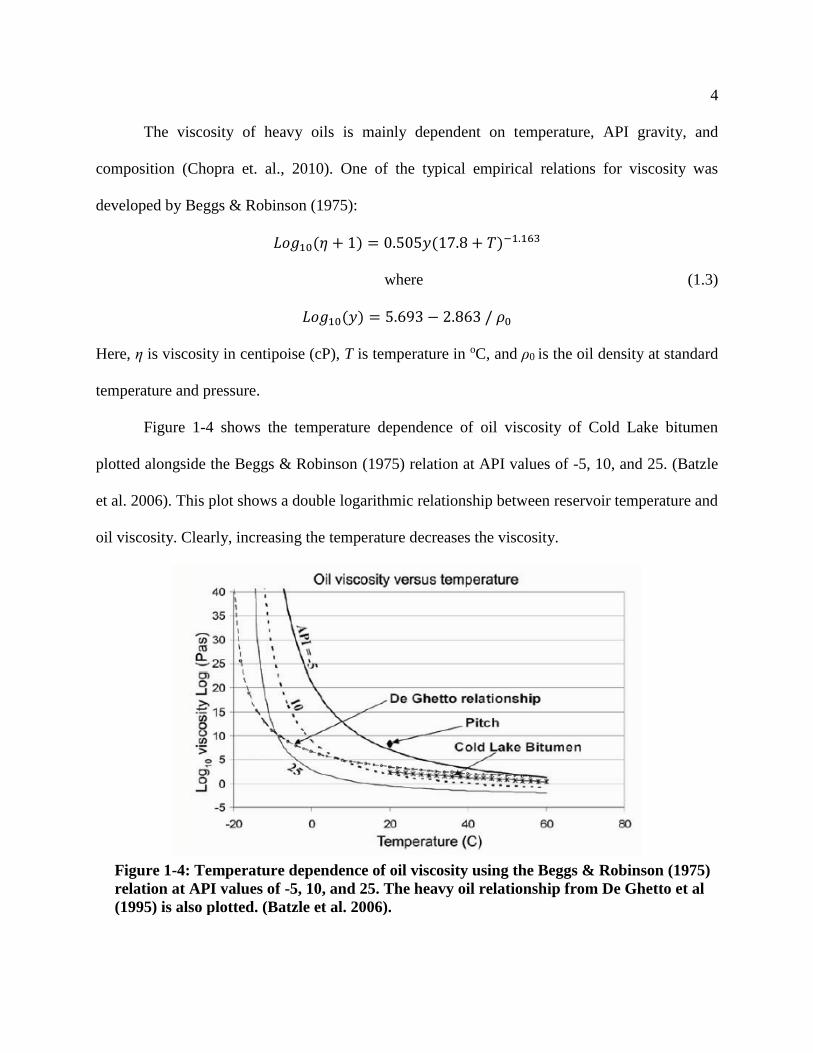
The viscosity of heavy oils is mainly dependent on temperature, API gravity, and

composition (Chopra et. al., 2010). One of the typical empirical relations for viscosity was

developed by Beggs & Robinson (1975):

𝐿𝑜𝑔10(𝜂 + 1) = 0.505𝑦(17.8 + 𝑇)−1.163

where (1.3)

𝐿𝑜𝑔10(𝑦) = 5.693 − 2.863 / 𝜌0

Here, η is viscosity in centipoise (cP), T is temperature in oC, and ρ0 is the oil density at standard

temperature and pressure.

Figure 1-4 shows the temperature dependence of oil viscosity of Cold Lake bitumen

plotted alongside the Beggs & Robinson (1975) relation at API values of -5, 10, and 25. (Batzle

et al. 2006). This plot shows a double logarithmic relationship between reservoir temperature and

oil viscosity. Clearly, increasing the temperature decreases the viscosity.

Figure 1-4: Temperature dependence of oil viscosity using the Beggs & Robinson (1975)

relation at API values of -5, 10, and 25. The heavy oil relationship from De Ghetto et al

(1995) is also plotted. (Batzle et al. 2006).

5

1.2 – Shear properties of heavy oil

As the viscosity of heavy oil becomes high, it develops a non-negligible shear modulus

(Chopra et. al., 2010). This transition can be tested in the laboratory by propagating a shear wave

through the fluid sample. Batzle et. al., (2006) noticed for a very heavy oil sample (-5o API) at

low temperatures (-12.5 oC), a sharp shear-wave arrival is detected (Figure 1-5 right).

At this temperature, the oil is almost a solid and therefore has a shear modulus. As the

temperature is increased and the heavy oil becomes more fluid-like, the shear-wave velocity

decreases as well as its amplitude.

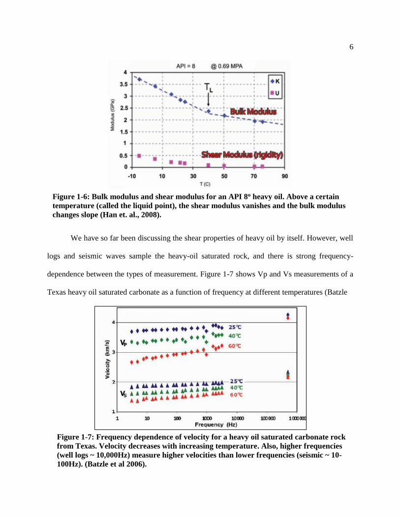
Figure 1-6 shows bulk and shear modulus lab measurements for an 8o API heavy oil (Han

et. at., 2008). At low temperatures, both bulk and shear moduli are present, but above a certain

temperature (called the liquid point), the shear modulus vanishes and the bulk modulus changes

slope. This analysis shows how heavy oil behaves like a viscoelastic material (semisolid) at

lower temperatures (high viscosities), and a viscous fluid at higher temperatures (Han et. al.,

2008).

Figure 1-5: Left – Ultrasonic compressional waveforms measured through a very heavy

oil (API = -5) at -12.5oC and 49.3oC. Right – Ultrasonic shear waveforms in the same

heavy oil at the same temperatures. Notice how in both cases, the waveform is both

delayed and attenuated at higher temperature (Batzle et. al., 2006).

6

We have so far been discussing the shear properties of heavy oil by itself. However, well

logs and seismic waves sample the heavy-oil saturated rock, and there is strong frequency-

dependence between the types of measurement. Figure 1-7 shows Vp and Vs measurements of a

Texas heavy oil saturated carbonate as a function of frequency at different temperatures (Batzle

Figure 1-6: Bulk modulus and shear modulus for an API 8o heavy oil. Above a certain

temperature (called the liquid point), the shear modulus vanishes and the bulk modulus

changes slope (Han et. al., 2008).

Figure 1-7: Frequency dependence of velocity for a heavy oil saturated carbonate rock

from Texas. Velocity decreases with increasing temperature. Also, higher frequencies

(well logs ~ 10,000Hz) measure higher velocities than lower frequencies (seismic ~ 10-

100Hz). (Batzle et al 2006).

7

et. al., 2006). Note the frequency dependence (dispersion) of both the P and S wave velocities,

which becomes more pronounced as temperatures increase. These observations clearly show how

velocities measured in the seismic band of 10–100 Hz do not agree with standard acoustic log

data (~10,000 Hz) nor with lab-measured ultrasonic (MHz-range) data (Batzle et. al., 2006).

This frequency-dependence (dispersion) of velocity is directly related to the attenuation

(Q factor) of the material. The Q factor can be related to the real and complex parts of the

dynamic shear modulus, as explained by Behura et. al. (2007), summarized below.

For a viscoelastic material subjected to a sinusoidal varying strain, the strain ε and

resulting stress σ can be represented by:

𝜖 = 𝜖0𝑒−𝑖𝜔𝑡 (1.4)

and

𝜎 = 𝜎0𝑒−𝑖(𝜔𝑡−𝛿) (1.5)

where ω = 2πf, 𝑖 = √−1, and δ is the phase lag. For an elastic material, the resulting stress is

instantaneous and so δ=0. For a purely viscous fluid, δ approaches π/2, whereas for a viscoelastic

body, δ lies in between the two limits. The complex dynamic shear modulus is given by:

�̃� =𝑠𝑡𝑟𝑒𝑠𝑠

𝑠𝑡𝑟𝑎𝑖𝑛= 𝐺′ + 𝑖𝐺′′ (1.6)

where

𝐺′ =𝜎0𝑐𝑜𝑠𝛿

𝜖0 (1.7)

and

𝐺′′ =𝜎0𝑠𝑖𝑛𝛿

𝜖0 (1.8)

G’ is the real part and is called the storage modulus, which represents the elastic component of

8

the material. G’’ is the imaginary part and is called the loss modulus, which represents the

viscous fluid component.

Integrating the out-of-phase component of stress over an entire cycle gives the energy

lost per cycle, and integrating the in-phase component of stress over a 1/4 full cycle gives the

maximum energy stored per cycle. As shown in Behura et. al. (2007), these integrations allow us

to derive Q as the ratio of the real and imaginary components of the complex shear modulus:

𝑄 =1

𝑡𝑎𝑛 𝛿=

𝑒𝑛𝑒𝑟𝑔𝑦

𝑒𝑛𝑒𝑟𝑔𝑦 𝑙𝑜𝑠𝑠(𝑝𝑒𝑟 𝑓𝑟𝑒𝑞𝑢𝑒𝑛𝑐𝑦 𝑐𝑦𝑐𝑙𝑒) =

𝐺′

𝐺′′ (1.9)

Behura et. al., (2007) performed lab measurements of G’ and Q (inversely proportional to

attenuation) of a heavy-oil saturated carbonate sample from Uvalde, Texas at varying

temperatures within the seismic frequency band. Their results are shown as color scaled three-

variable plots in Figure 1-8. G’ and Q show a moderate dependence on frequency but are

strongly influenced by temperature. G’ monotonically decreases with increasing temperature. As

for the quality factor, Q increases with frequency and initially decreases with temperature.

Figure 1-8: (Left): Storage modulus – temperature – frequency relation from lab

measurements of a heavy oil saturated carbonate from Uvalde, Texas. (Right): Quality

factor – temperature – frequency relation of the Uvalde heavy oil saturated carbonate.

Measurements were made at temperature increments of 10oC and frequency increments

of 0.1 on the Log10 scale (Behura et al 2007).

9

However, at higher temperatures, the Q trend reverses and begins to increase with increasing

temperatures. A likely explanation for this behavior is due to a loss of lighter hydrocarbon

components at high enough temperatures.

1.3 – Previous studies of estimating heavy oil viscosity

Several engineering-based empirical methods have been published to predict heavy oil

viscosity, such as the Beggs & Robinson (1975) relationship in Equation 1.3. However, the

author is only aware of two published methods where geophysical technology has been used to

predict heavy oil viscosity. Both of these methods are briefly summarized in this section.

Vasheghani & Lines (2012) developed a methodology to estimate viscosity from cross-

well seismic data between two wells by using traveltime tomography, attenuation tomography,

and rock physics (Figure 1-9). Since heavy oil is viscoelastic, the seismic energy attenuates with

propagation distance which can be measured in terms of the seismic quality factor Q. They

Figure 1-9: Viscosity tomogram from Vasheghani & Lines (2012).

10

related seismic Q to fluid viscosity in a two-stage process: First, they generated Q-tomograms

from the cross-well data using attenuation tomography with the frequency shift method.

Secondly, they related Q to fluid viscosity through the BISQ equations (Dvorkin et. al., 1994) to

create an estimated viscosity cross-section between the two study wells (Figure 1-9). There is

ambiguity, however, because for every Q value, two viscosity values can be calculated through

the BISQ equations. Also, there was no real viscosity data available for the authors to validate

their results against. Nevertheless, the work of Vasheghani & Lines (2012) demonstrates that

seismic data has potential to be used to estimate fluid viscosity in heavy oil reservoirs.

The second published method of estimating viscosity using geophysical technology is

through NMR well logging. Nuclear magnetic resonance (NMR) tools measure transverse

relaxation times (T2) of protons in rocks, and can be used to determine pore size distribution

(Rider & Kennedy 2011). A secondary parameter measured through NMR logging is the

Hydrogen Index (HI), which is a result of the signal amplitude being proportional to the amount

of hydrogen in the pore spaces (Rider & Kennedy 2011). Bryan et. al. (2005) demonstrated that

lab measured viscosities showed a correlation with these two NMR parameters (T2 and HI). They

showed that with increasing viscosity, T2 decreased, and at high viscosities T2 became less

sensitive to viscosity changes. However, increasing viscosities caused the decreasing HI to

become more sensitive to viscosity change at high viscosities. Based on these findings, Bryan et.

al. (2005) developed a new empirical relationship between the two NMR parameters and

viscosity, and adjusted it to provide the best possible fit to the database they were using, which

had oil viscosities from less than 1 cP to 3,000,000 cP. More studies (Sun et. al., 2007; Kantzas,

2009) have further developed on the NMR-viscosity correlation in the lab, all for the purpose of

11

developing a method to use downhole NMR measurements to predict viscosity down the

wellbore.

Figure 1-10 shows a heavy oil example from the Athabasca oil sands where lab viscosity

measurements were available from multiple samples down the wellbore. The empirical NMR-

viscosity relationship was used to generate a pseudo-viscosity log that showed fairly good

agreement with the lab viscosity measurements which ranged from 30,000 to 300,000 cP

(Alboudwarej et. al., 2006).

1.4 – Motivation and goals of this thesis

Reservoir fluid PVT (pressure-volume-temperature) properties, in particular fluid

viscosity, are crucial factors in selection of a recovery technique. For example, cold heavy-oil

production with sand (CHOPS) has been applied to reservoirs in Canada with oil viscosities

ranging from 50 to 15,000 cP (Alboudwarej et. al., 2006). However, recovery techniques cannot

Figure 1-10: A pseudo-viscosity log produced from two NMR logging parameters (T2

and HI), calibrated to laboratory viscosity measurements from the Athabasca oil sands

(Alboudwarej et. al. 2006).

12

be chosen solely based on viscosity ranges. Many factors must be taken into consideration such

as fluid properties, formation continuity, rock mechanics, drilling technology, completion

options, production simulation, surface facilities, reservoir thickness, and expected recovery and

production rates (Alboudwarej et. al., 2006). However, having an estimate of oil viscosity of a

reservoir beforehand will greatly aid in choosing the best recovery technique and determining

how to optimally produce the reservoir.

The only way to achieve a high degree of certainty on the viscosity of a heavy oil or oil

sands reservoir is by measuring the viscosity in the lab from core samples or wellhead oil

samples, which is an expensive undertaking (Miller et. al., 2006). It has been mentioned that the

signal from the NMR logging tool can be correlated to viscosity, however NMR logs are also

expensive and not commonly run. It would therefore be very useful to have a method to reliably

estimate viscosity using only standard well logs.

Donor Company has generously provided the author with lab viscosity measurements

from one of their major oil sands projects. The goal of this thesis is to investigate if a reasonable

correlation can be established between the measured viscosity values and the available well log

data, so that viscosity can be blindly predicted in nearby wells with a standard suite of well logs.

13

Chapter 2 – Well Logging Principles

2.1 – Overview of the well log measurement

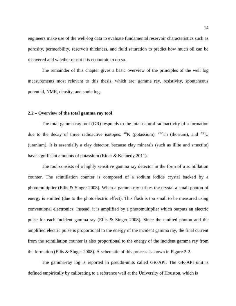
The continuous recording of a geophysical parameter down a borehole produces a

geophysical well log, more commonly referred as a well log. The logging tool is lowered down

the borehole by a spool and cable and measures different physical properties of the rocks as it is

pulled back up (Figure 2-1). For example, gamma-ray logs measure the natural radiation of the

formation, density and neutron logs calculate the porosity by measuring bulk density and

hydrogen concentrations, respectively, and resistivity logs measure the resistivities of the fluids

in the formation. From this data, geoscientists can infer lithological successions, depositional

environments, and fluid characteristics, which allow them to make predictions on where

petroleum accumulations are likely to exist. Once a reservoir is found, geoscientists and

Figure 2-1: The elements of well logging: the measurement tool (sonde) in a borehole,

the wireline pulled by a spool and cable, and the logging truck (Ellis & Singer, 2008).

14

engineers make use of the well-log data to evaluate fundamental reservoir characteristics such as

porosity, permeability, reservoir thickness, and fluid saturation to predict how much oil can be

recovered and whether or not it is economic to do so.

The remainder of this chapter gives a basic overview of the principles of the well log

measurements most relevant to this thesis, which are: gamma ray, resistivity, spontaneous

potential, NMR, density, and sonic logs.

2.2 – Overview of the total gamma ray tool

The total gamma-ray tool (GR) responds to the total natural radioactivity of a formation

due to the decay of three radioactive isotopes: 40K (potassium), 232Th (thorium), and 238U

(uranium). It is essentially a clay detector, because clay minerals (such as illite and smectite)

have significant amounts of potassium (Rider & Kennedy 2011).

The tool consists of a highly sensitive gamma ray detector in the form of a scintillation

counter. The scintillation counter is composed of a sodium iodide crystal backed by a

photomultiplier (Ellis & Singer 2008). When a gamma ray strikes the crystal a small photon of

energy is emitted (due to the photoelectric effect). This flash is too small to be measured using

conventional electronics. Instead, it is amplified by a photomultiplier which outputs an electric

pulse for each incident gamma-ray (Ellis & Singer 2008). Since the emitted photon and the

amplified electric pulse is proportional to the energy of the incident gamma ray, the final current

from the scintillation counter is also proportional to the energy of the incident gamma ray from

the formation (Ellis & Singer 2008). A schematic of this process is shown in Figure 2-2.

The gamma-ray log is reported in pseudo-units called GR-API. The GR-API unit is

defined empirically by calibrating to a reference well at the University of Houston, which is

15

made of large blocks of precisely known radioactivity’s ranging from very low to very high. The

scale is designed such that an “average shale” reads 100 GR-API (Rider & Kennedy 2011). Note

that the GR-API unit is completely unrelated to API gravity as discussed in chapter 1.

2.3 – Overview of the induction resistivity tool

The induction resistivity tool measures the conductivity of the invaded formation and

inverts it to obtain the resistivity value. The main application of the resistivity log is that it

provides information about the pore fluids (ie. if it is water or hydrocarbon bearing).

The tool consists of a transmitter coil and a receiver coil, illustrated in Figure 2-3. A high

frequency alternating current (AC) of about 20,000 Hz is applied to the transmitter coil, which

generates a magnetic field around it and induces secondary currents in the formation. These

currents flow in coaxial loops around the tool and create their own secondary magnetic field,

which induces currents in the receiver coil.

Figure 2-2: The life of a single gamma ray, which is emitted in the formation and

ultimately detected by a NaI detector in the borehole (Ellis & Singer 2008).

16

The voltage detected at the receiver is proportional to the conductivity of the formation

and to the square of the applied AC frequency, as given by (Ellis & Singer 2008):

𝑉𝑟𝑐𝑣𝑟 ∝ −𝜕(𝐵2)

𝜕𝑡∝ −𝜔2𝜎𝐼0𝑒−𝑖𝜔𝑡 (2.1)

where (B2)z is the vertical component of the secondary magnetic field in Teslas, ω is the

transmitter alternating current frequency in Hz, σ is the formation conductivity in mSiemens/m,

I0 is the transmitter current flow in Amperes, and 𝑖 = √−1.

As the hole gets drilled, the drilling mud can displace formation fluids in a

circumferential zone near the open borehole. This process is called invasion, which is illustrated

in Figure 2-4. The borehole wall acts like a filter, allowing the mud filtrate to invade the pores

immediately adjacent to the hole, and leaving the solid portion behind to coat the hole with “mud

cake.” Therefore, the completely invaded zone (“flushed zone”) will have different resistivity

Figure 2-3: The principle of the induction tool. The vertical component of the magnetic

field from the transmitter coil, Bt, induces ground current loops, J, in the formation.

These current loops in the conductive formation produce an alternating magnetic field,

B2, the vertical component of which is detected by the receiver coil (Ellis & Singer 2008).

17

characteristics than the uninvaded formation which is further away from the hole. Between these

two regions is a transitional zone of partial invasion (Schlumberger 2009).

The induction tool typically measures three resistivity curves: deep, medium, and

shallow. The deep curve measures the uninvaded zone (Rt), the medium curve measures the

transition zone, and the shallow curve measures the invaded zone RXO (Rider & Kennedy 2011).

In oil sands settings, invasion is minimal because of the highly viscous bitumen, and so

the three resistivity curves track each other closely (Cheng et. al., 2015).

2.4 – Overview of the spontaneous potential (SP) tool

The spontaneous potential (SP) log is a measurement of the natural potential differences

between an electrode in the borehole and a reference electrode at the surface. It can be used for

well-to-well correlation (though not as good as the gamma ray), estimating formation water

Figure 2-4: Borehole mud invasion profile:

“step model” of invasion

(adapted from Schlumberger 2009)

Nomenclature:

Borehole:

Rm = Resistivity of mud

Rmc = Resistivity of mud cake

Flushed (Invaded) Zone:

Rmf = Resistivity of mud filtrate

RXO = Resistivity of flushed zone

SXO = Water Saturation of flushed zone

Uninvaded or Virgin Zone:

Rt = True resistivity of formation

RW = Resistivity of formation water

SW = Formation water saturation

RS = Resistivity of adjacent (shoulder) bed

di = Diameter of invasion

dh = Borehole diameter

h = Bed thickness

18

resistivity (Rw), and as a permeability indicator (Rider & Kennedy, 2011).

Three factors are necessary to achieve an SP response: conductive drilling fluid in the

borehole, a porous and permeable bed surrounded by an impermeable formation, and a salinity

difference between the borehole fluid and the formation fluid (Rider & Kennedy 2011).

Consider a porous and permeable sandstone penetrated by a borehole, as shown in Figure

2-5. The mud filtrate is less saline than the sandstone formation water, therefore the mud filtrate

becomes negatively charged resulting in a negative SP deflection. Above the sandstone in the

semi-permeable shale, the borehole and formation salinities are similar and there is no SP

deflection. The greater the SP deflection, the greater the salinity contrast between the mud filtrate

and the formation water (Rider & Kennedy 2011).

Quantitatively, the SP can be used to estimate formation water resistivity using the

relationship between the resistivity and ionic activity (Rider & Kennedy 2011):

Figure 2-5: A schematic representation of the development of the spontaneous potential

signal in a borehole (modified from Ellis & Singer 2008).

19

𝑆𝑃 ≅ −𝐾𝑙𝑜𝑔𝑅𝑚𝑓

𝑅𝑤 (2.2)

where SP is the reading in mV, Rmf and Rw are the mud filtrate and formation water resistivities

in ohm*m, respectively, and K is a temperature constant (65 + 0.24(ToC)).

2.5 – Overview of the density logging tool

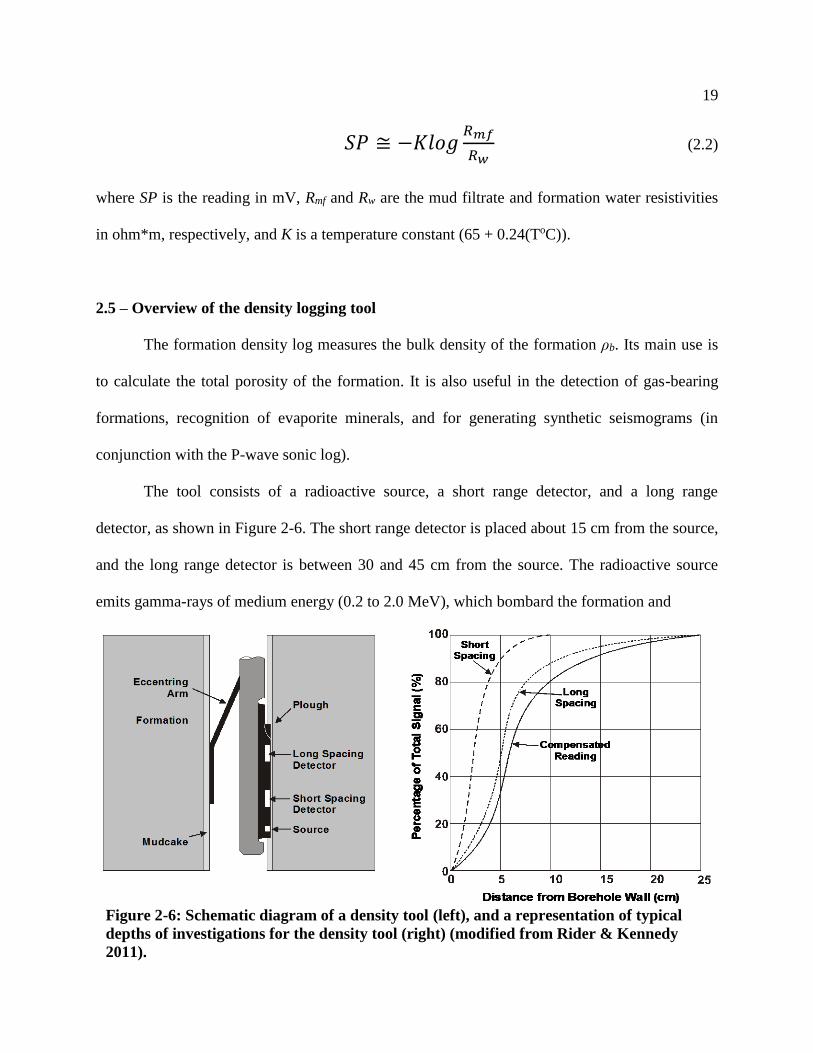
The formation density log measures the bulk density of the formation ρb. Its main use is

to calculate the total porosity of the formation. It is also useful in the detection of gas-bearing

formations, recognition of evaporite minerals, and for generating synthetic seismograms (in

conjunction with the P-wave sonic log).

The tool consists of a radioactive source, a short range detector, and a long range

detector, as shown in Figure 2-6. The short range detector is placed about 15 cm from the source,

and the long range detector is between 30 and 45 cm from the source. The radioactive source

emits gamma-rays of medium energy (0.2 to 2.0 MeV), which bombard the formation and

Figure 2-6: Schematic diagram of a density tool (left), and a representation of typical

depths of investigations for the density tool (right) (modified from Rider & Kennedy

2011).

20

undergo Compton scattering by interaction with the electrons inside the atoms of the formation.

This process reduces the energy of the gamma-rays and scatters them in all directions. The flux

of the gamma-rays returning to each of the two detectors is attenuated by an amount dependent

upon the electron density of the formation. Formations with a high bulk density have a high

electron density, which significantly attenuates the gamma rays to a low count rate being

recorded at the detectors. Formations with a low bulk density have a low electron density, which

attenuates the gamma-rays less resulting in a higher count rate (Rider & Kennedy 2011).

The electron density in a pure substance is directly related to its bulk density, described

the by relationship (Ellis & Singer 2008):

𝑛𝑒 =𝑁𝐴𝑍

𝐴𝜌𝑏 (2.3)

where ne is the electron number density of the substance in electrons/cm3, NA is Avogadro’s

number (6.022x1023), Z is the atomic number, A is the atomic weight in g/mol, and ρb is the bulk

density of the material in g/cm3. The gamma ray count at the detectors depends on the electron

density (related to the bulk density), as per the general attenuation relation (Ellis & Singer 2008):

𝑁 = 𝑁0𝑒−𝑛𝑒𝜎𝑥 (2.4)

where N is the counting rate of the detector at a distance x cm from the source, N0 is the natural

gamma-ray flux if there was no attenuation, and σ is the cross section for Compton scattering.

Figure 2-6 (right) also shows that over 80% of the signal from the short range detector

comes from within 5 cm of the borehole wall, which is mainly mudcake. For the long spacing

detector, about 80% of its signal comes from within 10 cm of the borehole wall. This is the

shallowest depth of investigation of all the standard logs (Rider & Kennedy 2011).

21

If the tool is flush against the borehole wall and there is no formation attenuation in the

near wellbore region, both detectors should give the same density. When the detectors measure

different densities, the difference is called the density correction, which arises due to mudcake or

mud filtrate invasion around the detectors. The density correction is applied to the raw

measurement and typically ranges from 0 to 1 g/cm3. In LAS files, the density correction curve is

usually available as a DRHO, ZCOR, or DENCOR curve name. Noisy behavior on the density

correction curve can indicate poor wellbore conditions, and potential for erroneous density

values (Rider & Kennedy 2011).

2.6 – Overview of the sonic logging tool

The sonic (or acoustic) log measures the slowness (reciprocal of velocity) of an acoustic

wave through a formation by recording the time for a pulse of sound to travel a known distance

through it. Sonic logs are primarily used for generating synthetic seismograms (in combination

with the density log) so that seismic data, measured in time, can be tied to wells, measured in

depth.

Three principal acoustic waves are detected in sonic logging: the compressional or P-

wave, the shear or S-wave, and the Stoneley wave, as shown in Figure 2-7 (Ellis & Singer 2008).

Compressional or P-waves are high in energy, low in amplitude, and caused by particle motion

in the direction of propagation. Shear waves or S-waves are associated with particle movement

perpendicular to the direction of propagation, and arrive after the compressional waves. The

Stoneley wave arrives after the shear wave, has less energy but a high amplitude which varies

with frequency, and is a complex type of surface wave. The Stoneley wave exists as a tube wave

22

in the cylindrical environment of the borehole (Rider & Kennedy 2011).

Older sonic tools (pre-1985) could measure only the P-wave arrival, but with the updated

technology of dipole sources, receiver arrays, and downhole digitization, the modern (array)

tools used today measure the full waveforms which provide the compressional, shear, and

Stoneley wave arrival times (Close et. al., 2009). The principles of the older tools will not be

discussed here.

The designs of sonic tools vary between logging companies, but all use an array of

receivers (between 8 and 13), and dipole transmitter sources. At each depth increment, the

transmitter emits a series of pulses at a frequency range exceeding 10,000 Hz. The refracted P-

and S-waves, and the borehole Stoneley waves are recorded by the receiver array (Figure 2-8).

The depth being sampled is at the midpoint of the array (Rider & Kennedy 2011).

Various signal processing algorithms exist to extract the slowness values from the series

Figure 2-7: A typical acoustic waveform recorded in a borehole. Three distinct arrivals

are indicated (Ellis & Singer 2008).

23

of waveforms, which make use of coherency methods. As an example, Schlumberger uses a

method called Slowness Time Coherency (STC), where a fixed-length time window is

incrementally advanced across the waveforms (Figure 2-9a). At each increment, the time-

window is rotated through the array in steps of increasing slowness (or increasing moveout) and

a coherency value is computed which represents how closely each moveout matches the

waveform. The coherency function is represented on the Z-axis of a slowness vs. time coherence

map for each measurement depth (Figure 2-9b). The coherence peaks are then plotted as points

on a log at each given depth (Figure 2-9c). Repeating this process at all depths is how P-wave

and S-wave slowness logs are created (Close et. al., 2009).

Computing the S-wave slowness values is less robust than calculating P-wave slowness

due to the problem of picking the shear-wave arrivals. In practice, the recorded waveforms are

not as clean as Figure 2-9a shows, and while the P-wave arrival is obtained from the first break

Figure 2-8: Simplified schematic of a sonic array logging system. At each sample depth, a

series of transmitter-common readings are made at different receiver offsets, where the

waveforms are digitally recorded by the receivers (modified from Smith et. al., 1991).

24

of each trace, the shear wave arrival is embedded in the mix of earlier arrivals. This introduces

more uncertainty into the S-wave slowness calculation (Lines et. al., 2010).

However, shear wave information has become critical in the last two decades for AVO

analysis, calculating reservoir geomechanical properties, detailed permeability analysis, and even

quantifying wellbore damage (Rider & Kennedy 2011). Despite the higher uncertainty in

measuring shear wave slowness, it is typically far superior to acquire a shear log instead of trying

to predict it from the compressional sonic log (Close et. al., 2009).

Figure 2-9: a) An array of waveforms showing increasing moveout from near to far

receivers. b) A slowness-time map in which coherent peaks correlate to different wave

components. c) A continuous log is built from repeating steps (a) and (b) at each depth

measurement point (modified from Close et. al., 2009).

25

2.7 – Overview of Nuclear Magnetic Resonance (NMR) logging

Unlike conventional logging measurements (ie. acoustic, density, and resistivity), which

respond to both the rock matrix and fluid properties and are strongly dependent on mineralogy,

NMR-logging measurements respond to the presence of hydrogen protons, which occur

primarily in pore fluids. NMR (nuclear magnetic resonance) provides information about the

quantities of fluids present, the properties of these fluids, and the pore size distributions

containing these fluids (Rider & Kennedy 2011).

The NMR measurement is extremely sensitive and complex. The heart of the

measurement involves measuring the characteristic decay time of protons, called the T2

relaxation time, by emitting a sequence of electromagnetic pulses at the correct Larmor

frequencies (Dunn et. al., 2002). In porous rocks, the protons lose their alignment (decay) by

surface relaxation as they collide with the solid, pore surface. In large pores, collisions will be

fewer and relaxation slower than in small pores. Essentially, the larger the pore, the longer the

decay time (Rider & Kennedy, 2011).

Figure 2-10 shows an idealized interpretation of the T2 distributions for water wet clastic

rocks (Ellis & Singer, 2008). Free, producible fluids (water or hydrocarbons) are found with T2

values greater than 33ms, while capillary bound water is found between 3ms and 33ms. The

components that decay faster than 3ms are attributed to clay-bound water, as illustrated in Figure

2-10 (Ellis & Singer, 2008). These T2 cutoff values are the basis for most NMR interpretation in

clastic reservoirs around the world.

26

Figure 2-11 shows a typical display of NMR data. The right side track shows the T2

distribution at each depth. The left track shows the three NMR porosities calculated from the T2

amplitudes. The rightmost curve is the sum of amplitudes greater than 33ms (moveable fluid

porosity). Between this lower limit and the middle dotted line, shaded in very light grey is the

additional contribution between 3 and 33 ms (capillary bound water). The dark shaded region

beyond corresponds to the porosity with T2 less than 3 ms (clay bound water).

Figure 2-10: A summary of the idealized interpretation of T2 distributions for water wet

clastic rocks (Ellis & Singer, 2008).

27

In bitumen settings, the NMR response is more complicated. Due to the extremely high

viscosities, the T2 decay times are so low (on the order of 1 ms) to the point where NMR cannot

detect the bitumen at all (Ellis & Singer, 2008). The simplest way to find bitumen is to compare

the density porosity log (which sees all porosity), to the NMR total porosity (which does not see

the bitumen), as shown in Figure 2-12.

Figure 2-12 shows an example well from the study area, with the NMR total, NMR free,

and moveable fluid porosities plotted. The dark grey area represents the bitumen in the smallest

pores and capillaries (not seen by the NMR). The magenta area represents hydrocarbon with

poor mobility in small pores and capillaries that the NMR can see. Green represents free

(moveable) fluid in the small to medium pores, and cyan represents free, moveable fluids in the

larger pores. However, these are not true representations of moveable porosities because NMR

cannot see most of the hydrocarbon porosity in bitumen settings (Bob Everett, retired

Schlumberger petrophysicist, personal communication, November 2016).

Figure 2-11: NMR T2 distributions as a function of depth are shown in the right track.

The left track shows the moveable-fluid (right curve), capillary-bound (middle curve),

and total (left curve) porosities calculated from the T2 amplitudes (Ellis & Singer, 2008).

28

Figure 2-12: Oil sands well in the study area with NMR data. The density porosity and

NMR total porosity curves diverge in the bitumen zones. The grey filled area is bitumen,

the magenta area is hydrocarbon in small pores and capillaries, the green area is free

hydrocarbon in medium pores, and blue represents free fluids in the larger pores (seen by

NMR). Figure generated in Hampson-Russell™ software.

29

Chapter 3 – Theory of Multilinear Regression

3.1 – Multi-Attribute Analysis

One way of measuring the correlation between a single attribute and the target attribute is

to cross-plot them, in which case the best fit is a 2D line. If we cross-plot two attributes against

the target attribute, the best fit is a plane, as shown in Figure 3-1. (Hampson-Russell 2016).

Figure 3-2 illustrates the basic multi-attribute problem, showing the target log and, in this

case, three attribute logs to be used to predict the target attribute (Hampson-Russell 2016).

Figure 3-1: (Left): Cross-plotting

against 1 attribute gives a line best fit.

(Right): Cross-plotting against 2

attributes gives a planar best fit

(Hampson-Russell 2016).

Figure 3-2: The basic multi-attribute regression problem showing the target log and in

this example, the 3 attributes to be used to predict the target (Hampson-Russell 2016).

30

To illustrate the theory of multi-attribute prediction, let us assume the target log is P-

wave velocity, attribute 1 is bulk density, attribute 2 is gamma-ray, and attribute 3 is resistivity.

The goal in this example is to predict P-wave velocity (in the depth domain) from the bulk

density, gamma-ray, and resistivity curves.

We can write the fundamental equation for linear prediction as:

𝑉𝑝(𝑧) = 𝑤0 + 𝑤1𝐷(𝑧) + 𝑤2𝐺(𝑧) + 𝑤3𝑅(𝑧) (3.1)

where Vp(z) is P-wave velocity in m/s, D(z) is bulk density in kg/m3, G(z) is gamma-ray in GR-

API units, and R(z) is resistivity in ohm*m. This can be written as a series of linear equations:

NNNN RwGwDwwVp

RwGwDwwVp

RwGwDwwVp

3210

23222102

13121101

(3.2)

where each row of equations represents a single depth increment. This can also be written in

matrix form:

[

𝑉𝑝1

𝑉𝑝2

⋮𝑉𝑝𝑁

] = [

1 𝐷1 𝐺1 𝑅1

1 𝐷2 𝐺2 𝑅2

⋮ ⋮ ⋮ ⋮1 𝐷𝑁 𝐺𝑁 𝑅𝑁

] [

𝑤0

𝑤1

𝑤2

𝑤3

]

or more compactly as:

𝑽𝒑 = 𝐴𝑾 (3.4)

We typically find that there are many more depth increments than the number of input

attributes. In other words, there are more rows in the A matrix than columns. This means that we

have an over-determined problem (more observations than unknowns), and the least-squares

solution is given by (Russell 2004):

(3.3)

31

𝑾 = [𝐴𝑇𝐴]−1𝐴𝑇𝑽𝒑 (3.5)

Applying these solved weights minimizes the squared error between Vp and AW:

|𝑽𝒑 − 𝐴𝑾|2 (3.6)

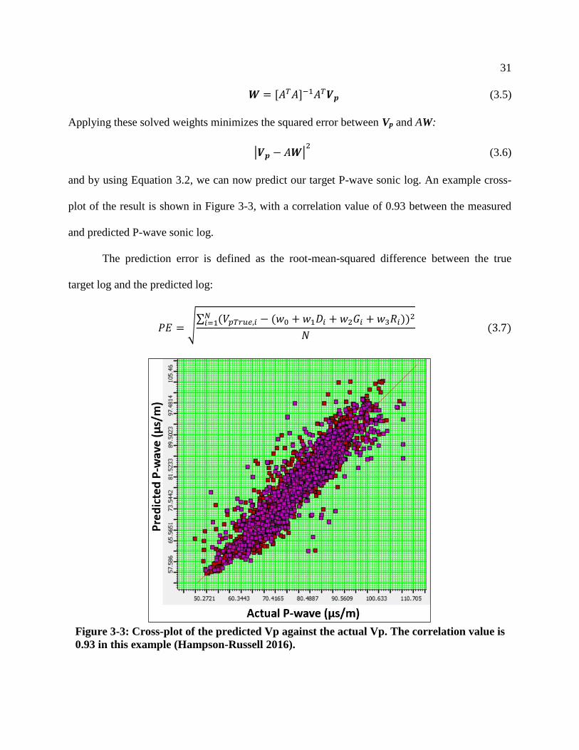
and by using Equation 3.2, we can now predict our target P-wave sonic log. An example cross-

plot of the result is shown in Figure 3-3, with a correlation value of 0.93 between the measured

and predicted P-wave sonic log.

The prediction error is defined as the root-mean-squared difference between the true

target log and the predicted log:

𝑃𝐸 = √∑ (𝑉𝑝𝑇𝑟𝑢𝑒,𝑖 − (𝑤0 + 𝑤1𝐷𝑖 + 𝑤2𝐺𝑖 + 𝑤3𝑅𝑖))2𝑁

𝑖=1

𝑁 (3.7)

Figure 3-3: Cross-plot of the predicted Vp against the actual Vp. The correlation value is

0.93 in this example (Hampson-Russell 2016).

32

or more simply:

𝑃𝐸 = √∑ (𝑉𝑝𝑇𝑟𝑢𝑒,𝑖 − 𝑉𝑝𝑃𝑟𝑒𝑑𝑖𝑐𝑡𝑒𝑑,𝑖)2𝑁

𝑖=1

𝑁 (3.8)

where N is the number of depth increments in the well that we use to train our correlation.

3.2 – Step-Wise Regression

In the previous section we showed that P-wave velocity could be predicted using three

attributes (density, gamma-ray, and resistivity). However, these might not be the best attributes

to use for the prediction. Hampson-Russell’s Emerge™ software uses a process called step-wise

regression to find the combination of attributes that is most useful for predicting the target log.

Step-wise regression can be nicely explained in a series of steps (Russell 2004):

1. Find the single best attribute by trial and error. In other words, calculate the prediction

error for each individual attribute. The best attribute is the one with the lowest prediction

error. Call this attribute A1.

2. Find the best pair of attributes. In other words, form all pairs of attributes including A1:

(A1, gamma-ray); (A1, resistivity); (A1, neutron porosity); and so on. The pair with the

lowest prediction error is the best pair. Call this second attribute A2.

3. Find the best triplet of attributes. In other words, form all triplets of attributes including

A1 and A2: (A1, A2, resistivity); (A1, A2, neutron porosity); and so on. The triplet with

the lowest prediction error is the best triplet. Call this third attribute A3.

4. Carry on this process until all the available attributes are used.

33

An important point to note is that the prediction error will always decrease (or stay the

same) as we increase the number of attributes (Russell 2004). However, the validation error does

not always decrease as we add attributes, which is addressed in the following section.

3.3 – Cross-Validation

Step-wise regression will give us a set of attributes that is guaranteed to reduce the total

error as the number of attributes goes up. So when do we stop? This is determined using a

technique called cross-validation, where we leave out a training well and predict it from the

remaining wells (Russell 2004).

Suppose we use five wells to train our correlation: Well1, Well2, Well3, Well4, Well5.

Cross-validation works in the following steps (Hampson-Russell 2016):

1. Leave out Well1, and solve for the regression coefficients using only data from (Well2,

Well3, Well4, Well5). In other words, solve the system of equations from Equation 3.2

where the rows contain no data from Well1.

2. With these coefficients, calculate the prediction error for Well1 (Equation 3.7 or 3.8),

where now only data points from Well1 are used. This gives us the validation error for

Well1. Denote it as VE1.

3. Repeat this process for Well2, Well3, Well4, and Well5, each time leaving the selected well

out in the calculation of regression coefficients, but using only that well for the error

calculation.

4. Calculate the average validation error for all wells:

𝑉𝐸𝑎𝑣𝑔 =𝑉𝐸1 + 𝑉𝐸2 + 𝑉𝐸3 + 𝑉𝐸4 + 𝑉𝐸5

5 (3.9)

34

In this example, the validation error computation was done using three attributes.

However, it is routinely performed after each stage of the step-wise regression procedure, so that

we have the average validation error as a function of the number of attributes. A validation plot

for an Emerge™ analysis is shown in Figure 3-4.

The horizontal axis shows the number of attributes used for the prediction, and the

vertical axis shows the root-mean-square prediction error for that number of attributes (Equation

3.8). The lower black curve shows the error calculated using the training data (all of the wells).

The upper red curve shows the error calculated using the validation data (by systematically

leaving out wells and calculating the average validation error). This particular example shows

that when greater than four attributes are used, the validation error starts to increase, which

means that any additional attributes will over-fit the data (Russell 2004).

Figure 3-4: An Emerge™ prediction error plot. (Hampson-Russell 2016).

35

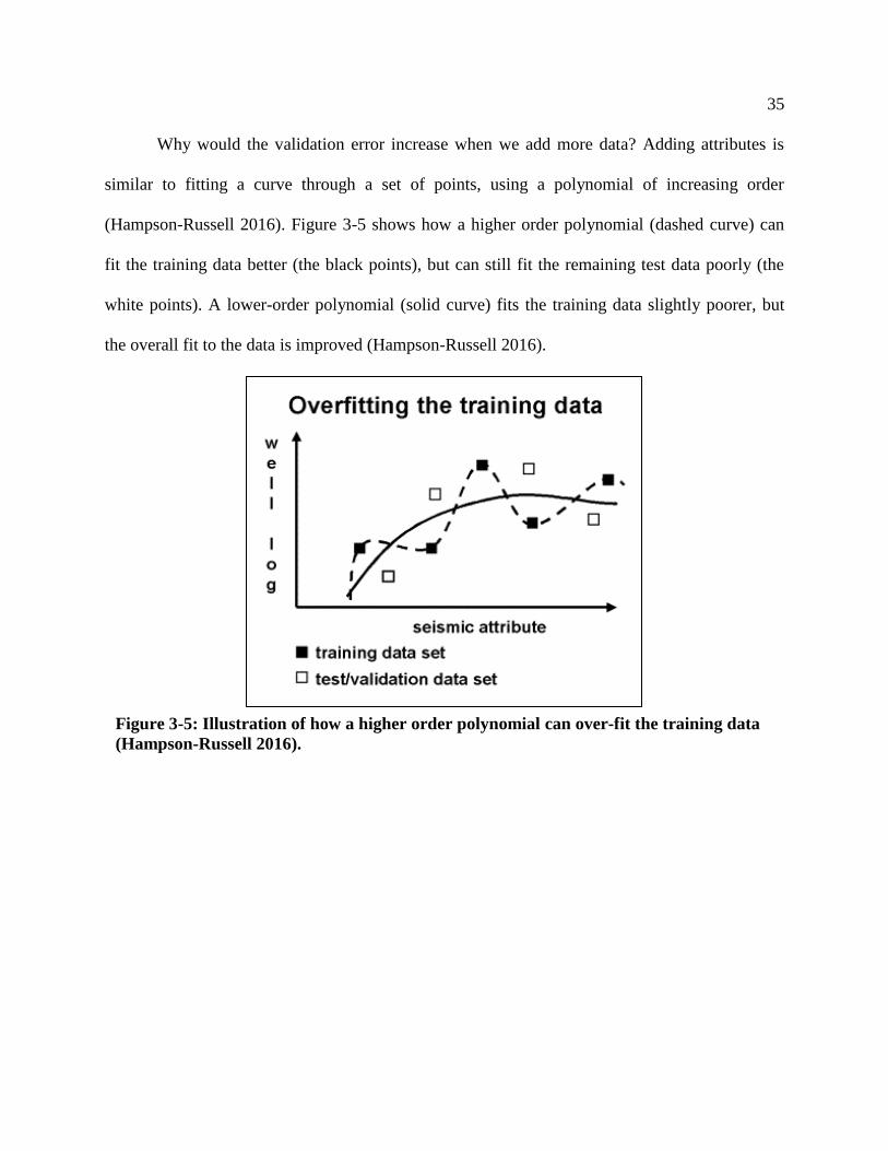
Why would the validation error increase when we add more data? Adding attributes is

similar to fitting a curve through a set of points, using a polynomial of increasing order

(Hampson-Russell 2016). Figure 3-5 shows how a higher order polynomial (dashed curve) can

fit the training data better (the black points), but can still fit the remaining test data poorly (the

white points). A lower-order polynomial (solid curve) fits the training data slightly poorer, but

the overall fit to the data is improved (Hampson-Russell 2016).

Figure 3-5: Illustration of how a higher order polynomial can over-fit the training data

(Hampson-Russell 2016).

36

Chapter 4 – Study Area Geology and Dataset

4.1 – Introduction to Study Area

The study area for this thesis is located within the Athabasca oil sands of Alberta, in the

vicinity of Fort McMurray. Athabasca is the largest oil sands deposit, followed by Cold Lake and

Peace River (Figure 4-1). The data donor has requested that the exact project location remain

confidential.

The reservoir of interest is the McMurray Formation, a bitumen saturated reservoir

situated about 200m to 350m below the surface. Production of the viscous bitumen is ongoing

Figure 4-1: Distribution of Alberta’s oil sands deposits (Norman Einstein, Own work,

Public Domain, https://commons.wikimedia.org/w/index.php?curid=773312).

37

through steam-assisted gravity drainage (SAGD) which uses pairs of horizontal steam injection

and producing wells drilled through the McMurray formation reservoir to mobilize the bitumen.

The reservoir sands are hosted in stacked channel deposits, separated by silty or muddy intervals

(Hein et. al. 2013).

Bitumen of the Athabasca region is heavy and largely immobile due to extensive

biodegradation, containing in-situ viscosities from 100,000 cP to over 1,000,000 cP, and API

gravities from 8o to 10o, in comparison to conventional oil with API gravities from 24o to 40o

(Mossop, 1980). The sand grains of the bitumen reservoir are water wet, a key element which

makes steam injection recovery possible. Oil saturation levels vary, containing up to 20%

bitumen by weight (Mossop, 1980).

Average reservoir effective porosities in the study area are on the order of 30%, with an

average shale volume of 11% and permeability in the range of 4800-6300 mD. Water saturation

levels average 32%, and in-situ reservoir temperatures are about 10oC at pressures from 1000-

1100 kPa (Kelly, 2012).

4.2 – Study Area Geology

The stratigraphic units of the Athabasca oil sands system comprise of the Cretaceous

siliciclastic rocks and the underlying Devonian carbonates. Figure 4-2 shows a simplified

stratigraphic column highlighting the three intervals of interest: the Beaverhill Lake Group

carbonates, the McMurray Formation reservoir, and the Clearwater Formation caprock. The units

will be described here from the bottom up, using the example well log suite from Figure 4-3 to

support the descriptions. This particular well was chosen because it is one of the few wells that

has log data reaching the top of the Devonian carbonates.

38

Below the bitumen reservoir sits the Beaverhill Lake Group carbonates, consisting of

Devonian age dolomites, limestones, and evaporates (Schneider et. al., 2012). They are

characterized by a high degree of deformation and karsting due to dissolution of the Prairie

Evaporite Formation salts (situated directly underneath the Beaverhill Lake Group). The result is

a complex surface with varying structural highs and lows (Schneider et. al., 2012). The upper

boundary of the Beaverhill Lake Group is defined by the sub-Cretaceous unconformity. It is an

angular unconformity representing an ~ 250Ma hiatus of sedimentation, with extensive erosion

and karsting (Hein et. al., 2013). The sub-Cretaceous unconformity represents an ancient

Figure 4-2: Stratigraphic chart for the McMurray oil sands system (Nexen AER Report,

2015).

39

paleo-geographic erosional surface containing escarpments, faults, sinkholes, and collapse

features (Schneider et. al., 2012). The structure of the sub-Cretaceous unconformity is important

to understand since it heavily influences the deposition of the overlying McMurray Formation

sediments.

The transition from the McMurray Formation sands to the Beaverhill Lake Group

carbonates is easily identified from logs (Figure 4-3 at 235m). There are abrupt decreases in the

P- and S-wave slownesses, and in the density porosity (meaning increasing density), plus an

increase on the photoelectric curve from 2 barns/electron (indicating sandstone) to 5

barns/electron (indicating limestone). Sonic logs are usually plotted with slowness increasing to

the left (ie. velocity increasing to the right). For an illustration of how the Vp/Vs ratio behaves,

refer to Figure 5-6 in chapter 5.

Figure 4-3: Log suite for an example well in the study area, from the Clearwater

Formation caprock down to the Beaverhill Lake Group carbonates. The depth units are

in meters. Figure plotted in MATLAB®.

40

The McMurray Formation is the main bitumen reservoir throughout the Athabasca region

and the focus point of this study. It is characterized by continental successions of fine to very

fine-grained sands with mixed-in conglomerates and mudstones (Mossop, 1980). It was

deposited in a N-S trending incised valley or depression on top of the sub-Cretaceous

unconformity, created from dissolution of the Prairie River Evaporite salts and resulting collapse

of the overlying formations (Hein et. al., 2013). In the Cretaceous period, a large fluvial system

shaped the underlying carbonates into a distribution of structural highs and lows. The lows play a

key role in the amount of reserves in the McMurray Formation, because the sediments that were

deposited in lows host most of the bitumen. The thickness of the McMurray is dependent on the

Devonian structure, varying from 150m thick in the centre of deposition to where it pinches out

in the west against a ridge of Devonian limestone (Flach, 1984). The stratigraphic framework of

the McMurray is shown in Figure 4-4.

The McMurray is usually divided into a Lower and an Upper section. The Lower

McMurray is comprised of fluvial sediments with sand dominated channels and point-bar

complexes with high porosities and permeabilities. These lowermost sediments are called the

McMurray C channel deposits. They directly overlay the sub-Cretaceous unconformity. In some

regions, channel fill from the Upper McMurray almost entirely erodes through the Lower

McMurray to the sub-Cretaceous unconformity. These sediments are simply called McMurray

channel sediments (Hein et. al., 2013).

The Upper McMurray is split into A and B sequences, which mainly consist of coastal

plain and estuarine successions, respectively, containing channel fill and point bar complexes

with lower porosities and permeabilities than in the Lower McMurray (Hein et. al., 2013). The

41

channel fills contain a mixture of mudstones and point bar sands, which are often bitumen-

saturated. The mudstones are commonly present in the form of inclined heterolithic stratification

(IHS), which are typically thick and discontinuous fills from abandoned channels, acting as

baffles to steam-chamber flow (Hein et. al., 2013). Due to the shallow depth of the McMurray

(lack of burial), the bitumen sands are unconsolidated (Mossop, 1980).

In the study area, the bitumen saturated zones are mostly confined in the mid to lower

levels of the McMurray. This is demonstrated in Figure 4-3 from the low (sand) gamma-ray

response, porosities greater than 30%, high resistivity readings, and the weight % bitumen

(WTAR) curve from 200m to 230m. Note that it is not a homogeneous sand unit, there are

several thin shaley zones in between the clean sands. Figure 4-2 shows a wet sand layer

underneath the oil sands layer because water is present underneath the bitumen in some, but not

all places throughout the study area. The well from Figure 4-3 does not have bottom water, but

Figure 4-4: Stratigraphic framework for the McMurray Formation and Wabiskaw

member in the Athabasca region of Alberta (Hein et. al., 2013).

42

several wells in the area do have bottom water ranging from thin to 20m thick.

Lastly, the viscosity samples in this study encompass the bitumen-saturated zones in the

mid to lower McMurray (Figure 4-3), and viscosity appears to increase with depth in most cases.

The Clearwater Formation conformably overlies the McMurray reservoir throughout the

Athabasca region. The base of the Clearwater Formation contains the Wabiskaw Member, a

glauconitic sandstone with interbedded shales, that acts as a secondary target for oil sands

extraction (Hein et. al., 2013). The rest of the Clearwater Formation is largely heterogeneous,

containing fine-grained marine shales with intermixed silt and sands (Flach, 1984). The fine-

grained shales form the caprock of the McMurray reservoir, providing a vertical seal for the oil

prior to biodegradation, and presently serves as a vertical barrier preventing steam from

migrating upward.

In the study area, there is a shaley-sand wet zone in the Upper Clearwater, seen from

120m to 130m depth in the example well (Figure 4-3). The caprock interval in the study area is

defined as the interval from the shale beneath this wet zone down to the Wabiskaw sand zone, as

annotated in Figure 4-3.

4.3 – Dataset

A focused map of the oil sands study area is shown in Figure 4-5. In the area, there are 78

total wells with viscosity measurements, shown by the large well symbols. 40 of these wells have

full suites of logs, highlighted by the large red symbols. These 40 wells were used to train the

viscosity prediction, as described in chapter 5. All wells here with viscosity measurements were

vertically drilled. The wells each have had cores taken from the McMurray formation. The

bitumen was extracted from the cores by a 3rd party laboratory and the kinematic viscosities were

43

measured at 35oC, 55oC, and 75oC. The measurements at 35oC were used for this study which

most closely resembles reservoir conditions. The majority of wells have 3 viscosity

measurements: shallow, middle, and base reservoir samples as in Figure 4-3.

Figure 4-6 shows a histogram of all the viscosity samples throughout the study area. The

viscosities range from 10,000 cP to 550,000 cP, with an average value of 121,000 cP and

standard deviation of 100,000 cP.

Figure 4-7 shows the distribution of the base reservoir viscosity measurements,

interpolated between wells using a standard minimum curvature algorithm in SeisWare™. There

are significant lateral viscosity variations throughout the reservoir. If we could predict these

variations from well logs before developing the reservoir (the focus for the next chapter), it

would greatly help in determining the optimal recovery method, amount of steam to inject, and

well placement.

Figure 4-5: Map of the oil sands study area. The large well symbols are the 78 wells with

viscosity measurements. The large red well symbols are the 40 corresponding wells that

also contain a full suite of logs. These 40 wells were used to train the viscosity prediction.

Figure generated in SeisWare™

44

Figure 4-6: Histogram of all laboratory viscosity measurements throughout the study area.

Figure 4-7: Distribution map of the base reservoir viscosity measurements. All the data

wells are shown in red (generated in SeisWare™).

45

Chapter 5 – Problem Setup, and Viscosity Prediction Results

5.1 – Well log normalization process

Before performing quantitative analysis on well logs (such as prediction), the logs should

all be normalized. Well log normalization identifies and removes systematic errors from well log

data so that reliable results may be obtained for reservoir evaluation, solving difficult correlation

and quantitative problems. Reasons for tool inaccuracies include varying borehole conditions

from well to well, improper wellsite tool calibrations, or logs from different logging companies

in the same area (Shier, 2004).

There are a number of methods for normalizing logs within a cluster of wells. For this

study the “Big Histogram Method” was used, which adjusts the logs within a zone of interest to

all have the same average and standard deviation value from well to well (Shier, 2004). Figure

5-1 illustrates this concept for the gamma ray logs. The histogram shows the distribution of

gamma ray values for the 40 project wells from top to base of the gross bitumen interval.

The gamma ray logs for each well were then adjusted so that the average and standard

deviation values matched the global average (44 and 15.5 GR-API respectively) using the

Figure 5-1: Distribution of the gamma ray values for the 40 training wells from top to

base of the gross bitumen interval. Each color represents a different well. Figure created

in Hampson-Russell™ software.

46

normalization equation at each depth sample:

𝑂𝑢𝑡𝑝𝑢𝑡(𝑖) =𝐿𝑜𝑔𝑉𝑎𝑙𝑢𝑒(𝑖) − 𝐴𝑣𝑒𝑟𝑎𝑔𝑒

𝑆𝑡𝑑𝐷𝑒𝑣(𝐷𝑒𝑠𝑖𝑟𝑒𝑑𝑆𝑡𝑑𝐷𝑒𝑣) + 𝐷𝑒𝑠𝑖𝑟𝑒𝑑𝑀𝑒𝑎𝑛 (5.1)

where Average and StdDev represent the average and standard deviation values of the log in a

specific well, and DesiredStdDev and DesiredMean represent the global values that each well is

adjusted to match.

Figure 5-2 shows an example well of how the normalized logs (red) compare to the un-

normalized logs (blue). The normalized logs resemble bulk shifted versions of the original logs

to match the global average, with some slight character changes to match the global standard

deviation. To normalize the resistivity logs, the base 10 logarithm of resistivity was normalized

and converted back to ohm*m units, since resistivity has a logarithmic scale.

Figure 5-2: What the normalized logs look like (red) versus the un-normalized logs (blue).

The normalization was focused from top to base of the gross bitumen interval. The gold

zones highlight the bitumen intervals.

47

5.2 – Adding NMR logs as viscosity predicting attributes

It is already known that the NMR logging response can be correlated to viscosity, as

discussed in section 1.3. The purpose of incorporating NMR data into this study was to see if

combining NMR with the other well logs improves the data-driven viscosity prediction.

Donor Company has generously provided all of their wells in the study area that have

NMR data. Unfortunately, none of the 25 provided NMR wells have viscosity measurements.

Therefore, the 25 NMR wells were used the find the best NMR prediction model from the

remaining well logs. The prediction model was then used to blindly predict the NMR logs in

each of the 40 viscosity wells to see if the predicted NMR logs would improve the viscosity

prediction. Quite an ambitious, and possibly laughable, task.

Table 5-1, Table 5-2, and Table 5-3 show the Emerge™ top predicting attributes for

NMR total porosity, NMR free porosity, and NMR moveable water, respectively. Note that each

row corresponds to a particular multi-attribute transform and includes all the rows above it.

Target (%) Attribute Units Validation Error (%)

1 NMR Total Porosity 1 / (Medium Resistivity) 1 / (ohmm) 3.47

2 NMR Total Porosity (P-wave sonic)1/2 (µs/m)1/2 3.23

3 NMR Total Porosity ln |Gamma Ray| ln|GR-API| 2.96

Table 5-1: Emerge™ top predicting attributes for NMR Total Porosity.

Target (%) Attribute Units Validation Error (%)

1 NMR Free Porosity 1 / (Medium Resistivity) 1 / (ohmm) 3.53

2 NMR Free Porosity (P-wave sonic)2 (µs/m)2 3.28

3 NMR Free Porosity Gamma Ray GR-API 3.09

Table 5-2: Emerge™ top predicting attributes for NMR Free Porosity.

Target (%) Attribute Units Validation Error (%)

1 NMR Moveable Fluid 1 / (Medium Resistivity) 1 / (ohmm) 3.45

2 NMR Moveable Fluid (Density)1/2 (kg/m3)1/2 3.17

3 NMR Moveable Fluid 1 / (Neutron Porosity) 1 / (decimal) 2.93

4 NMR Moveable Fluid (P-wave sonic)2 (µs/m)2 2.79

Table 5-3: Emerge™ top predicting attributes for NMR Moveable Fluid Porosity.

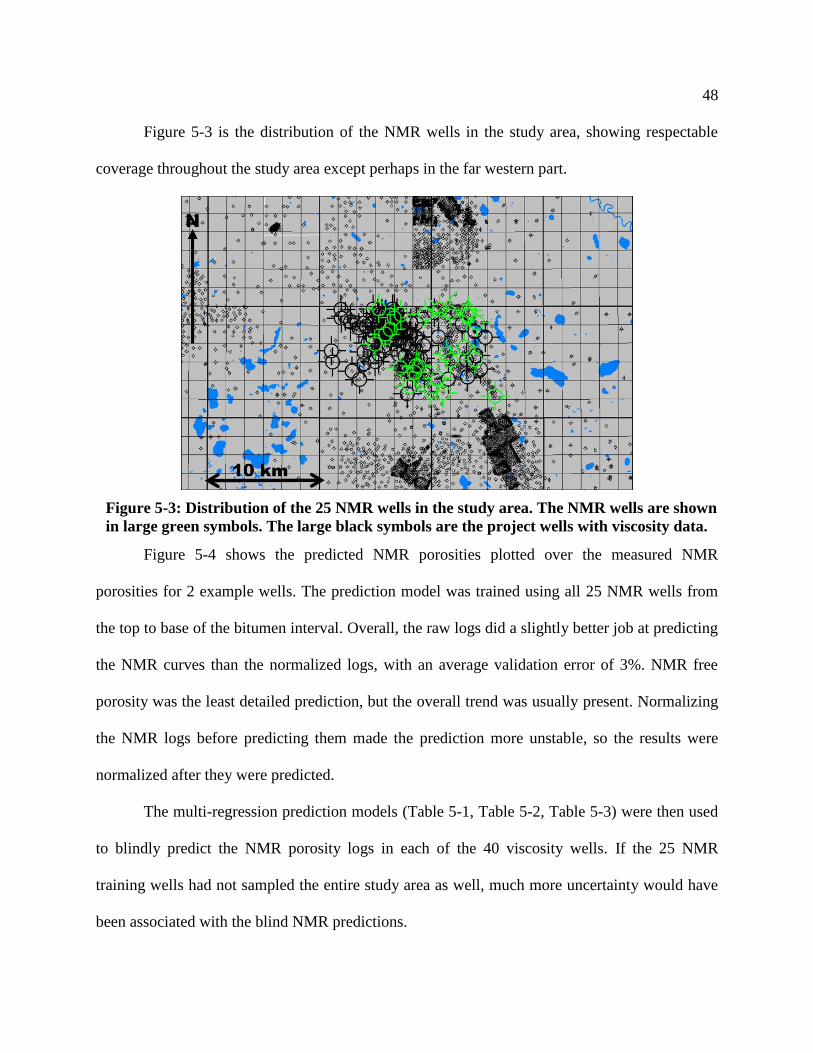
48

Figure 5-3 is the distribution of the NMR wells in the study area, showing respectable

coverage throughout the study area except perhaps in the far western part.

Figure 5-4 shows the predicted NMR porosities plotted over the measured NMR

porosities for 2 example wells. The prediction model was trained using all 25 NMR wells from

the top to base of the bitumen interval. Overall, the raw logs did a slightly better job at predicting

the NMR curves than the normalized logs, with an average validation error of 3%. NMR free

porosity was the least detailed prediction, but the overall trend was usually present. Normalizing

the NMR logs before predicting them made the prediction more unstable, so the results were

normalized after they were predicted.

The multi-regression prediction models (Table 5-1, Table 5-2, Table 5-3) were then used

to blindly predict the NMR porosity logs in each of the 40 viscosity wells. If the 25 NMR

training wells had not sampled the entire study area as well, much more uncertainty would have

been associated with the blind NMR predictions.

Figure 5-3: Distribution of the 25 NMR wells in the study area. The NMR wells are shown

in large green symbols. The large black symbols are the project wells with viscosity data.

49

5.3 – Viscosity training model

In order to train a multi-attribute relationship how to predict viscosity from other logs, we

had to create viscosity target logs for the Hampson-Russell Emerge™ database. This was done

for each of the 40 training wells (Figure 4-5) using two different methods: in the first method, the

target viscosity logs were created by linear interpolation between each viscosity measurement

point, and nulling the log everywhere outside of the reservoir interval. This is shown in the left

track of Figure 5-5 for an example well, where the three viscosity measurements are denoted by

the blocked red log, and the black curve shows the interpolated target viscosity log.

The second method creates the target viscosity log using a 1-meter training window

centered around the true measurement depths, as shown by the gold zones in Figure 5-5.

Figure 5-4: Predicting NMR porosities from Resistivity, P-wave sonic, Gamma Ray, and

Neutron Porosity. Validation results for two example wells are shown. Each of the 25

NMR wells were systematically left-out and predicted from the remaining 24 wells. The

black curves are the measured NMR porosities, the red curves are the predicted NMR

porosities using normalized logs, and the green curves are the predicted NMR porosities

using the un-normalized (raw) logs. Credit: Hampson-Russell Emerge™

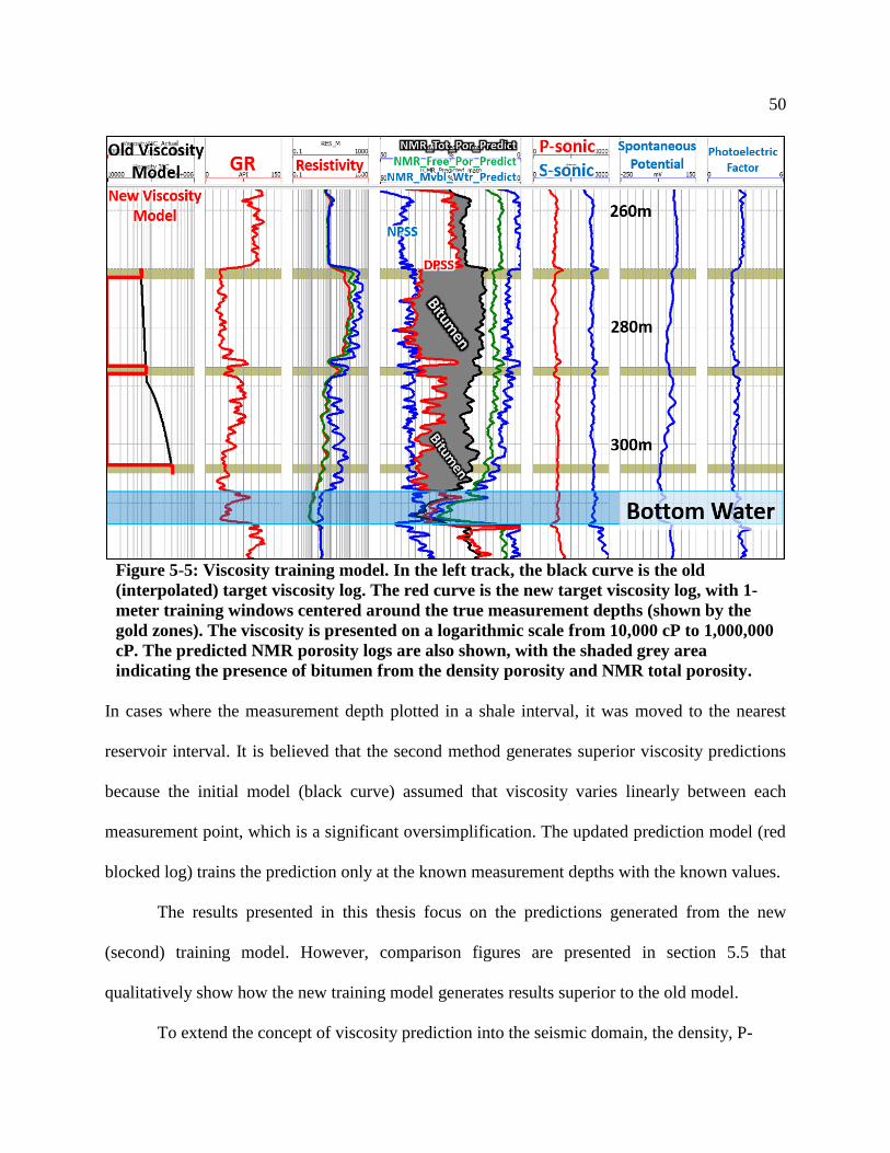
50

In cases where the measurement depth plotted in a shale interval, it was moved to the nearest

reservoir interval. It is believed that the second method generates superior viscosity predictions

because the initial model (black curve) assumed that viscosity varies linearly between each

measurement point, which is a significant oversimplification. The updated prediction model (red

blocked log) trains the prediction only at the known measurement depths with the known values.

The results presented in this thesis focus on the predictions generated from the new

(second) training model. However, comparison figures are presented in section 5.5 that

qualitatively show how the new training model generates results superior to the old model.

To extend the concept of viscosity prediction into the seismic domain, the density, P-

Figure 5-5: Viscosity training model. In the left track, the black curve is the old

(interpolated) target viscosity log. The red curve is the new target viscosity log, with 1-

meter training windows centered around the true measurement depths (shown by the

gold zones). The viscosity is presented on a logarithmic scale from 10,000 cP to 1,000,000

cP. The predicted NMR porosity logs are also shown, with the shaded grey area

indicating the presence of bitumen from the density porosity and NMR total porosity.

separation.

51

wave, and the S-wave sonic logs were used to calculate the following seismic properties in the

40 project wells: P-impedance, S-impedance, Bulk Modulus, Shear Modulus, Vp/Vs, Young’s

Modulus, Poisson’s Ratio, P-Elastic Impedance, and PS-Elastic Impedance. These properties

were used as predicting attributes to generate a separate viscosity prediction in each well, using

only log-derived seismic properties. The setup of the training model was exactly the same as the

one described above, only the predicting attributes have changed (Figure 5-6).

5.4 – Viscosity prediction results using all logs, and calculated seismic properties

Upon running the multi-linear regression analysis in Hampson-Russell’s Emerge™

software (as explained in chapter 3), the top viscosity predicting attributes were determined.

Figure 5-6: Viscosity training model using only log-derived seismic properties. In the left

track, the black curve is the old (interpolated) target viscosity log. The red curve is the

new target viscosity log, with 1-meter training windows centered around the true

measurement depths (shown by the gold zones). The viscosity is presented on a

logarithmic scale from 10,000 cP to 1,000,000 cP.

52

Figure 5-7 shows the graphical training and validation errors from using all available well

logs as predicting attributes, along with the list of the attributes in descending order of

importance. The results show the optimum viscosity prediction is made using the top six

attributes. The validation error curve remains almost flat beyond six attributes, indicating that the

prediction would be over-trained beyond six attributes. The average validation error is 69,300 cP,

which is 0.693 of one standard deviation of all measured viscosity values. The correlation value

of the predicted viscosities versus the measured viscosities is 0.76.

Target (cP) Final Attribute Units Validation Error (cP)

1 Viscosity 1 / (Medium Resistivity) 1 / (ohmm) 84,200

2 Viscosity ln(Gamma Ray) ln(GR-API) 76,600

3 Viscosity (NMR TotalPor – FreePor)1/2 (decimal)1/2 74,300

4 Viscosity 1 / (SP) 1 / (mV) 71,800

5 Viscosity 1 / (P-wave sonic) 1 / (μs/m) 71,100

6 Viscosity 1 / (S-wave sonic) 1 / (μs/m) 69,300

Figure 5-7: Top: Emerge™ prediction error plot and cross-plot for viscosity using the new

training model, and all the available well logs as the predicting attributes. In the

crossplot, each color represents a different well. Bottom: The list of attributes with their

associated validation errors. Note that each row in the list corresponds to a particular

multi-attribute transform and includes all the attributes above it. Explicit prediction

equation is A1.1 in appendix A1.

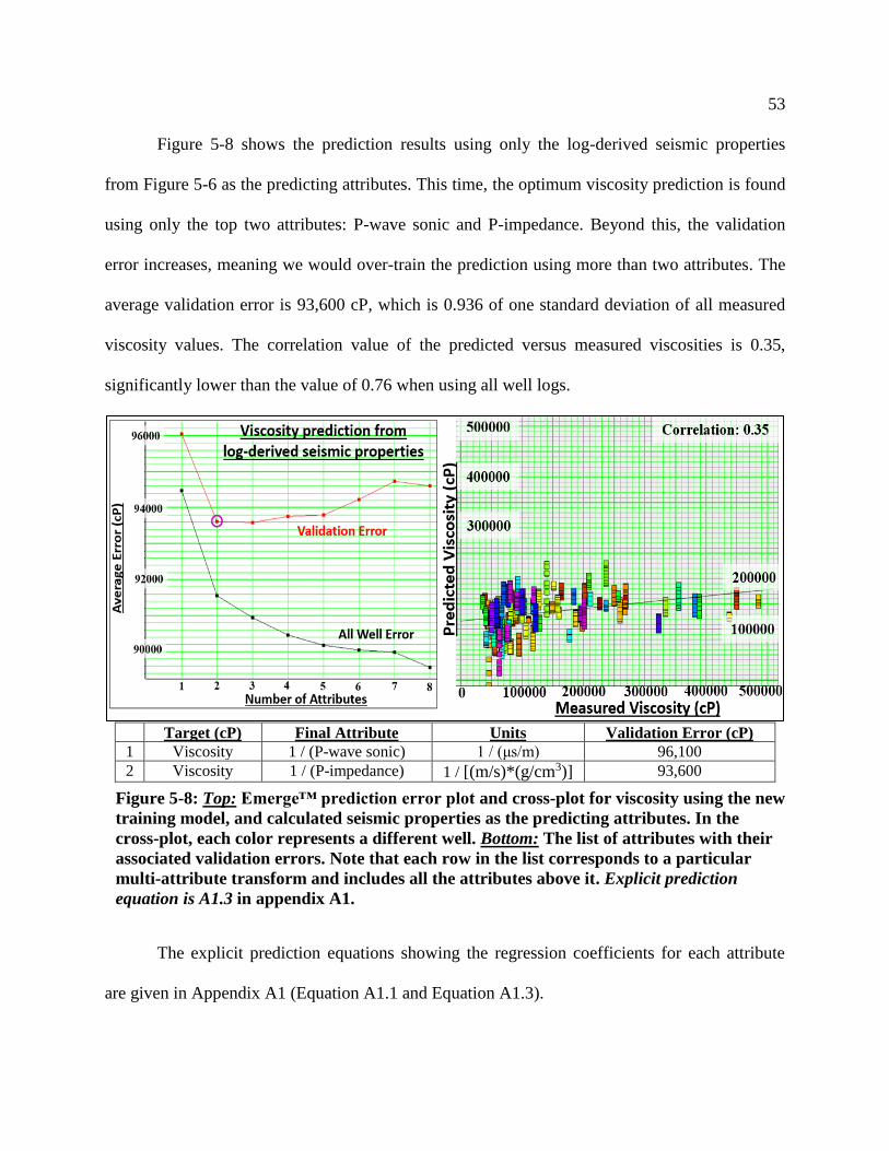
53

Figure 5-8 shows the prediction results using only the log-derived seismic properties

from Figure 5-6 as the predicting attributes. This time, the optimum viscosity prediction is found

using only the top two attributes: P-wave sonic and P-impedance. Beyond this, the validation

error increases, meaning we would over-train the prediction using more than two attributes. The

average validation error is 93,600 cP, which is 0.936 of one standard deviation of all measured

viscosity values. The correlation value of the predicted versus measured viscosities is 0.35,

significantly lower than the value of 0.76 when using all well logs.

Target (cP) Final Attribute Units Validation Error (cP)

1 Viscosity 1 / (P-wave sonic) 1 / (μs/m) 96,100

2 Viscosity 1 / (P-impedance) 1 / [(m/s)*(g/cm3)] 93,600

The explicit prediction equations showing the regression coefficients for each attribute

are given in Appendix A1 (Equation A1.1 and Equation A1.3).

Figure 5-8: Top: Emerge™ prediction error plot and cross-plot for viscosity using the new

training model, and calculated seismic properties as the predicting attributes. In the

cross-plot, each color represents a different well. Bottom: The list of attributes with their

associated validation errors. Note that each row in the list corresponds to a particular

multi-attribute transform and includes all the attributes above it. Explicit prediction

equation is A1.3 in appendix A1.

54

5.5 – Visualizing the viscosity predictions

This section is a series of figures to illustrate how the viscosity predictions actually

behave in a few example wells. In each figure, the leftmost track shows the viscosity predictions

using all well logs (from Figure 5-7), and the rightmost track shows the predictions using

calculated seismic properties (from Figure 5-8). The true viscosities are superimposed in black

for comparison. The gold zones highlight the reservoir intervals, and the magenta colored area is

the separation between the predicted NMR Total and NMR Free porosity logs (the 3rd top

predictor). For terminology, the “old prediction” refers to predictions using the old, interpolated

training model (Figure 5-5 black curve). The “new prediction” refers to predictions using the

updated, blocked training model (Figure 5-5 red log).

Figure 5-9 shows a well with bitumen extending 20m above the shallowest viscosity

measurement. Both predictions (using well logs and calculated seismic properties) show good

agreement with the measured viscosities, and they both predict a smooth trend of decreasing

viscosity to the top of the bitumen reservoir. The spikes in the predicted viscosity logs occur in

non-reservoir intervals, which makes sense because the predictions are only trained at the

measurement points, all occurring in reservoir intervals. There is relatively little difference

between the old and new viscosity predictions in this well.

Figure 5-10 shows a well with more dynamic behavior of the modeled viscosity. On the

left side (prediction using well logs), the new viscosity prediction shows more variation than the

old prediction. The new model shows a shallow decreasing viscosity profile from 410m to 420m,

and three separate profiles of increasing viscosity in three reservoir intervals (430m to 460m)

separated by shalier intervals, showing good agreement with the measured viscosities. This

behavior of increasing viscosity gradients has been documented in other areas of the

55

Athabasca oil sands (Larter et. al., 2008). It is encouraging that similar behavior is modelled here

from well logs in the study area. In the right track of Figure 5-10, the viscosity prediction from

calculated seismic properties shows less variation, and does not see the same trends. Note that

most of the spikes in the predicted viscosities occur in the shaley zones. This is not a problem

because we care only about the viscosity in the reservoir intervals.

Figure 5-11 shows a well with two viscosity gradients predicted from well logs (left

side). One from 215m to 233m, and the other from 235m to 245m. The predicted viscosity

closely matches the true viscosity at each of the three measurement depths. On the right side, the

viscosity prediction from calculated seismic properties detects less variation than the well logs

see, but still matches the true viscosities within reason.

Figure 5-12 shows a well where the predicted viscosity from well logs (left side) models

a smooth increasing gradient from the top to base of the reservoir. There is a beautiful inverse

correlation between the resistivity curve and the viscosity values. This inverse trend is

observable in most wells (though not in Figure 5-9), and is the reason why resistivity emerged as

the most important viscosity predicting attribute (Figure 5-7). The viscosity prediction from

calculated seismic properties (right side) unfortunately does not model this trend so nicely.

In general, it has been observed that the new predictions yield greater viscosity variations

than the old predictions. These variations are those we might expect to see in stacked bitumen

intervals separated by shale layers. On the other hand, the viscosity predictions using calculated

seismic properties detect less vertical variation than the well logs see, with higher validation

error. This is not surprising since the prediction from seismic properties had a correlation value

of only 0.35, compared to 0.76 when using all the well logs.

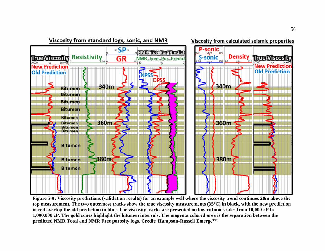
56

Figure 5-9: Viscosity predictions (validation results) for an example well where the viscosity trend continues 20m above the

top measurement. The two outermost tracks show the true viscosity measurements (350C) in black, with the new prediction

in red overtop the old prediction in blue. The viscosity tracks are presented on logarithmic scales from 10,000 cP to

1,000,000 cP. The gold zones highlight the bitumen intervals. The magenta colored area is the separation between the

predicted NMR Total and NMR Free porosity logs. Credit: Hampson-Russell Emerge™

57

Figure 5-10: Viscosity predictions (validation results) for an example well where three viscosity gradients are modelled

from 430m to 460m, separated by shaley zones. The two outermost tracks show the true viscosity measurements (350C) in

black, with the new prediction in red overtop the old prediction in blue. The viscosity tracks are presented on logarithmic

scales from 10,000 cP to 1,000,000 cP. The gold zones highlight the bitumen intervals. The magenta colored area is the

separation between the predicted NMR Total and NMR Free porosity logs. Credit: Hampson-Russell Emerge™

58

Figure 5-11: Viscosity predictions (validation results) for an example well where two viscosity gradients are modelled

throughout the reservoir interval. The two outermost tracks show the true viscosity measurements (350C) in black, with the

new prediction in red overtop the old prediction in blue. The viscosity tracks are presented on logarithmic scales from

10,000 cP to 1,000,000 cP. The gold zones highlight the bitumen intervals. The magenta colored area is the separation

between the predicted NMR Total and NMR Free porosity logs. Credit: Hampson-Russell Emerge™

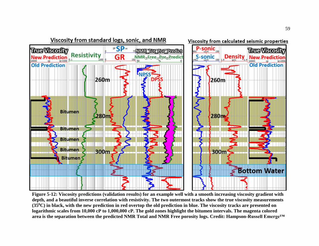
59

Figure 5-12: Viscosity predictions (validation results) for an example well with a smooth increasing viscosity gradient with

depth, and a beautiful inverse correlation with resistivity. The two outermost tracks show the true viscosity measurements

(350C) in black, with the new prediction in red overtop the old prediction in blue. The viscosity tracks are presented on

logarithmic scales from 10,000 cP to 1,000,000 cP. The gold zones highlight the bitumen intervals. The magenta colored

area is the separation between the predicted NMR Total and NMR Free porosity logs. Credit: Hampson-Russell Emerge™

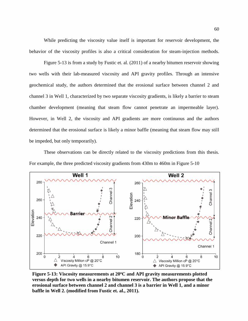
60

While predicting the viscosity value itself is important for reservoir development, the

behavior of the viscosity profiles is also a critical consideration for steam-injection methods.

Figure 5-13 is from a study by Fustic et. al. (2011) of a nearby bitumen reservoir showing

two wells with their lab-measured viscosity and API gravity profiles. Through an intensive

geochemical study, the authors determined that the erosional surface between channel 2 and

channel 3 in Well 1, characterized by two separate viscosity gradients, is likely a barrier to steam

chamber development (meaning that steam flow cannot penetrate an impermeable layer).

However, in Well 2, the viscosity and API gradients are more continuous and the authors

determined that the erosional surface is likely a minor baffle (meaning that steam flow may still

be impeded, but only temporarily).

These observations can be directly related to the viscosity predictions from this thesis.

For example, the three predicted viscosity gradients from 430m to 460m in Figure 5-10

Figure 5-13: Viscosity measurements at 20oC and API gravity measurements plotted

versus depth for two wells in a nearby bitumen reservoir. The authors propose that the

erosional surface between channel 2 and channel 3 is a barrier in Well 1, and a minor

baffle in Well 2. (modified from Fustic et. al., 2011).

61

resemble the gradients from Well 1 of Fustic et. al. (2011), which suggests that the shaley zones

at 440m and 450m could act as steam barriers. These viscosity gradients were hardly seen from

the old prediction of Figure 5-10 (blue curve), which further supports that the new prediction is

superior to the old prediction.

The smooth predicted viscosity gradient from Figure 5-12 resembles Well 2 from Fustic

et. al. (2011), which suggests the shaley zones throughout the reservoir could act more as minor

steam baffles, only temporarily impeding steam flow. A similar conclusion can be made

regarding the shaley zone at 240m in Figure 5-11.

5.6 – Viscosity prediction using only standard logs, and predicting log10(viscosity)

Due to cost, most wells do not have sonic logs, and far fewer have NMR logs. Therefore,

another set of viscosity predictions were generated using only the standard, most commonly-run

logs as the predicting attributes: gamma-ray, resistivity, density, neutron porosity, spontaneous

potential, and the photoelectric curve.

This section also compares the prediction of viscosity versus the prediction of

log10(viscosity). Since viscosity is a logarithmic variable (with respect to temperature),

predicting the log10(viscosity) might be a more robust approach. This was done by forcing

Emerge™ to predict log10(viscosity) as the target attribute, then converting back to linear space

by 10^[predicted log10(viscosity)] to compare with the absolute viscosity predictions.

Figure 5-14 shows the graphical training and validation errors from using only the

standard well logs as predicting attributes, along with the list of attributes in descending order of

importance. The result shows that the optimum viscosity prediction is made using the top three

attributes. Beyond this, the validation error increases, meaning we would over-train the

62

prediction using more than three attributes. The average validation error is 74,600 cP, which is

0.75 of one standard deviation of all the measured viscosity values, and only 5,300cP greater

than using all the well logs. The correlation value is 0.70, not much worse than the 0.76 value

from using all well logs. The prediction equation is given in appendix A1 (Equation A1.2).

Target (cP) Final Attribute Units Validation Error (cP)

1 Viscosity 1 / (Medium Resistivity) 1 / (ohmm) 84,200

2 Viscosity ln(Gamma Ray) ln(GR-API) 76,600

3 Viscosity 1 / (SP) 1 / (mV) 74,600

Figure 5-15 and Figure 5-16 show comparisons of the three viscosity prediction methods:

using all available well logs (from Figure 5-7), using only standard well logs (from Figure 5-14),

and using log-derived seismic properties (from Figure 5-8). Also plotted as the green curves are

the log10(viscosity) predictions converted back to linear space.

There is little noticeable difference between the prediction using all well logs (left track)

and the prediction using standard well logs (middle track). Using all well logs gives a slightly

more accurate prediction, as seen by inspecting the viscosity measurement at 230m in

Figure 5-14: Top: Emerge™ prediction error plot and cross-plot for viscosity using the

new training model, and only the standard logs as predicting attributes. In the crossplot,

each color represents a different well. Bottom: The list of attributes with their associated

validation errors. Note that each row in the list corresponds to a particular multi-

attribute transform and includes all the attributes above it. Explicit prediction equation is

A1.2 in appendix A1.

63

Figure 5-15: Comparison of the three viscosity prediction methods for an example well.

The predicted log10(viscosity) converted back to linear space is shown in green. The

bitumen intervals are highlighted in gold.

Figure 5-16: Comparison of the three viscosity prediction methods for an example well.

The predicted log10(viscosity) converted back to linear space is shown in green. The

bitumen intervals are highlighted in gold.

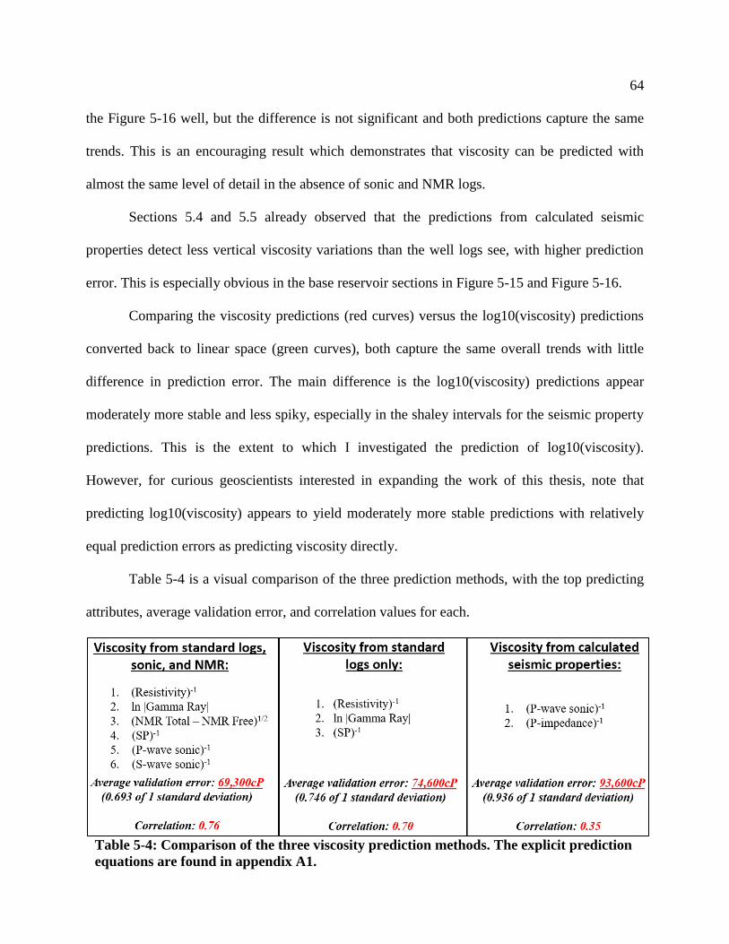
64

the Figure 5-16 well, but the difference is not significant and both predictions capture the same

trends. This is an encouraging result which demonstrates that viscosity can be predicted with

almost the same level of detail in the absence of sonic and NMR logs.

Sections 5.4 and 5.5 already observed that the predictions from calculated seismic

properties detect less vertical viscosity variations than the well logs see, with higher prediction

error. This is especially obvious in the base reservoir sections in Figure 5-15 and Figure 5-16.

Comparing the viscosity predictions (red curves) versus the log10(viscosity) predictions

converted back to linear space (green curves), both capture the same overall trends with little

difference in prediction error. The main difference is the log10(viscosity) predictions appear

moderately more stable and less spiky, especially in the shaley intervals for the seismic property

predictions. This is the extent to which I investigated the prediction of log10(viscosity).

However, for curious geoscientists interested in expanding the work of this thesis, note that

predicting log10(viscosity) appears to yield moderately more stable predictions with relatively

equal prediction errors as predicting viscosity directly.

Table 5-4 is a visual comparison of the three prediction methods, with the top predicting

attributes, average validation error, and correlation values for each.

Table 5-4: Comparison of the three viscosity prediction methods. The explicit prediction

equations are found in appendix A1.

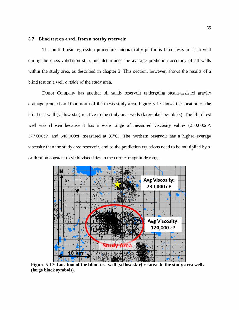
65

5.7 – Blind test on a well from a nearby reservoir

The multi-linear regression procedure automatically performs blind tests on each well

during the cross-validation step, and determines the average prediction accuracy of all wells

within the study area, as described in chapter 3. This section, however, shows the results of a

blind test on a well outside of the study area.

Donor Company has another oil sands reservoir undergoing steam-assisted gravity

drainage production 10km north of the thesis study area. Figure 5-17 shows the location of the

blind test well (yellow star) relative to the study area wells (large black symbols). The blind test

well was chosen because it has a wide range of measured viscosity values (230,000cP,

377,000cP, and 640,000cP measured at 35oC). The northern reservoir has a higher average

viscosity than the study area reservoir, and so the prediction equations need to be multiplied by a

calibration constant to yield viscosities in the correct magnitude range.

Figure 5-17: Location of the blind test well (yellow star) relative to the study area wells

(large black symbols).

66

Figure 5-18 shows the viscosity predictions in the blind test well by applying a

calibration constant of 4.0 to the well log prediction equations, and a calibration constant of 2.8

to the log-derived seismic properties prediction. The measured viscosities are shown by the black

dots, with the predicted viscosities superimposed. Unlike the wells in the study area, here, the

best prediction comes from log-derived seismic properties, which models an increasing viscosity

gradient with depth matching the measured values reasonably well. Most of the spikes in the

prediction occur within interbedded shale intervals.

Through correspondence with Donor Company geoscientists, the resistivity, SP, and S-

wave sonic logs are less consistent and less reliable throughout this northern reservoir than in the

study area. The prediction equation from log-derived seismic properties (P-wave sonic and

Figure 5-18: Prediction results in the blind test well 10km north of the study area. This

northern reservoir has a higher average viscosity than the study area reservoir, so the

predictions were multiplied by constants to yield viscosities in the correct magnitude

ranges.

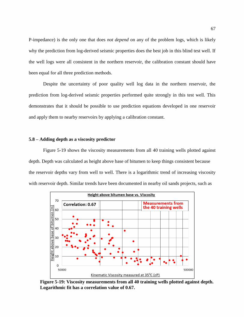
67

P-impedance) is the only one that does not depend on any of the problem logs, which is likely

why the prediction from log-derived seismic properties does the best job in this blind test well. If

the well logs were all consistent in the northern reservoir, the calibration constant should have

been equal for all three prediction methods.

Despite the uncertainty of poor quality well log data in the northern reservoir, the

prediction from log-derived seismic properties performed quite strongly in this test well. This

demonstrates that it should be possible to use prediction equations developed in one reservoir

and apply them to nearby reservoirs by applying a calibration constant.

5.8 – Adding depth as a viscosity predictor

Figure 5-19 shows the viscosity measurements from all 40 training wells plotted against

depth. Depth was calculated as height above base of bitumen to keep things consistent because

the reservoir depths vary from well to well. There is a logarithmic trend of increasing viscosity

with reservoir depth. Similar trends have been documented in nearby oil sands projects, such as

Figure 5-19: Viscosity measurements from all 40 training wells plotted against depth.

Logarithmic fit has a correlation value of 0.67.

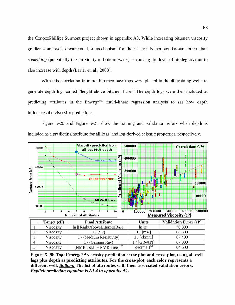
68

the ConocoPhillips Surmont project shown in appendix A3. While increasing bitumen viscosity

gradients are well documented, a mechanism for their cause is not yet known, other than

something (potentially the proximity to bottom-water) is causing the level of biodegradation to

also increase with depth (Larter et. al., 2008).

With this correlation in mind, bitumen base tops were picked in the 40 training wells to

generate depth logs called “height above bitumen base.” The depth logs were then included as

predicting attributes in the Emerge™ multi-linear regression analysis to see how depth

influences the viscosity predictions.

Figure 5-20 and Figure 5-21 show the training and validation errors when depth is

included as a predicting attribute for all logs, and log-derived seismic properties, respectively.

Target (cP) Final Attribute Units Validation Error (cP)

1 Viscosity ln |HeightAboveBitumenBase| ln |m| 70,300

2 Viscosity 1 / (SP) 1 / [mV] 68,300

3 Viscosity 1 / (Medium Resistivity) 1 / [ohmm] 67,400

4 Viscosity 1 / (Gamma Ray) 1 / [GR-API] 67,000

5 Viscosity (NMR Total – NMR Free)1/2 [decimal]1/2 64,600

Figure 5-20: Top: Emerge™ viscosity prediction error plot and cross-plot, using all well

logs plus depth as predicting attributes. For the cross-plot, each color represents a

different well. Bottom: The list of attributes with their associated validation errors.

Explicit prediction equation is A1.4 in appendix A1.

69

Target (cP) Final Attribute Units Validation Error (cP)

1 Viscosity ln |HeightAboveBitumenBase| ln |m| 70,300

2 Viscosity 1 / (P-wave sonic) 1 / [μs/m] 69,700

From Figure 5-20, including depth has improved the overall viscosity prediction using all

logs from 69,300cP to 64,600cP, and improved the correlation value from 0.75 to 0.79.

From Figure 5-21, including depth has improved the prediction using log-derived seismic

properties from 93,600cP to 69,700cP. However, the scaling on the error plot shows that

including seismic properties after depth does little to improve the overall prediction error.

Figure 5-22 shows visually how depth influences the viscosity prediction for three

example wells. It is generally observed that the predictions including depth (the red curves) are

closer to the true values than the predictions without depth (blue curves). The exception is the

well on the right, which has a low measured viscosity at the base (66,000cP at 440m depth),

whereas the depth predictor always expects viscosity to increase with depth (the green curve).

Figure 5-21: Top: Emerge™ viscosity prediction error plot and cross-plot, using log-

derived seismic properties plus depth as predicting attributes. For the cross-plot, each

color represents a different well. Bottom: The list of attributes with their associated

validation errors. Explicit prediction equation is A1.5 in appendix A1.

70

Figure 5-22: Influence of depth as a viscosity predictor for three example wells. In each well, the black blocked log shows

the true viscosity measurements, and the green logarithmic curve is the prediction using only depth. In the left tracks, the

viscosity predictions from all logs are plotted in blue, and the predictions from all logs plus depth are plotted in red. In the

right tracks, the viscosity predictions from calculated seismic properties are plotted in blue, and the predictions from seismic

plus depth are plotted in red. All tracks are presented on logarithmic scales from 10,000cP to 1,000,000cP. The gold zones

highlight the bitumen intervals. Credit: Hampson-Russell Emerge™

71

It is interesting to note for the left and middle wells in Figure 5-22, depth alone predicts the

measured viscosities almost perfectly as a logarithmic function (the green curves). However, this

loses all the high resolution detail obtained from well logs. Combining depth with the well logs

(red curves) captures the high resolution detail, while including the depth-viscosity trend from

Figure 5-19. This is somewhat a similar concept to adding the low frequency component for

seismic impedance inversions.

In summary, it was observed that including depth usually yields predictions closer to the

measured values, however depth will always overestimate viscosity in the special cases where

the base reservoir viscosity is low (as seen in the right well).

The results up to this point comprise the majority of the work done for this thesis. The

next sections outline two quick experiments I did to investigate how applicable seismic data

might be for predicting viscosity, and in detecting bitumen-water contacts.

5.9 – Predicting viscosity using acoustic logs filtered to seismic frequencies

This chapter has already shown the accuracy of using log-derived seismic properties to

predict viscosity. However, this was done at well logging frequencies on the order of 10,000Hz.

The P-wave sonic, S-wave sonic, and density logs were therefore low-pass filtered to 0–100/120

Hz as a proxy for what might be extracted from seismic inversion volumes. This process is

informally known as “upscaling” of well logs.

Table 5-5 shows the top viscosity predictors when the three upscaled acoustic logs are

Target (cP) Attribute Units Validation Error (cP)

1 Viscosity (upscaled P-wave sonic)2 (µs/m)2 95,700

2 Viscosity (upscaled S-wave sonic)2 (µs/m)2 94,700

3 Viscosity (upscaled density)2 (kg/m3)2 94,400

Table 5-5: Emerge™ top viscosity predicting attributes using acoustic logs upscaled to

seismic frequencies (lowpass filtered from 0 – 100/120 Hz, 1 ms sample rate).

72

input as the predicting attributes, using the same 40 training wells. Each attribute in turn slightly

reduces the validation error.

Figure 5-23 and Figure 5-24 show how the upscaled acoustic logs look relative to the

original logs, and how the viscosity predictions from upscaled acoustic logs look relative to the

original acoustic predictions (from Figure 5-8) for two example wells.

The well in Figure 5-23 has a fairly continuous 20m thick bitumen interval, seen from the

density log. The upscaled logs are smoothed versions of the originals. However, since this well

has a relatively continuous reservoir interval (which is rare for the study area), the upscaled logs

Figure 5-23: Predicting viscosity from upscaled acoustic logs for a well with a continuous

20m reservoir interval. The left track shows the true viscosity measurements in black,

with the upscaled acoustic prediction in blue overlaying the original acoustic prediction in

red. The other tracks show the upscaled acoustic logs in black overtop their original logs.

The bitumen interval is highlighted in gold. The logs were lowpass filtered from 0-

100/120Hz, with a 1ms sample rate.

73

still capture the main trends of the originals and the upscaled viscosity prediction is very similar

to the original acoustic viscosity prediction. This result suggests that using Vp, Vs, and density

inversion volumes may provide an estimate of viscosity variations in areas with relatively

continuous, thick reservoir.

Figure 5-24 shows the same results for a well with several interbedded shales throughout

the reservoir, seen from the density log spikes. In this well, the upscaled logs lose considerable

resolution because the frequent lithology changes are too thin to be detected at seismic

frequencies. As a result, the upscaled viscosity prediction is considerably less detailed than the

Figure 5-24: Predicting viscosity from upscaled acoustic logs for a well with several

interbedded shale intervals. The left track shows the true viscosity measurements in

black, with the upscaled acoustic prediction in blue overtop the original acoustic

prediction in red. The other tracks show the upscaled acoustic logs in black overtop their

original logs. The bitumen intervals are highlighted in gold. The logs were lowpass

filtered from 0-100/120Hz, with a 1ms sample rate.

74

original acoustic prediction. However, the upscaled prediction still matches the bottom two

measurements, and the curve itself appears to be a believable, smoothed gradient of increasing

viscosity with depth: still valuable information to have. The top reservoir prediction failed

because the thin, clean sand response at the top measurement point was completely filtered out in

each of the upscaled acoustic logs.

Both these examples suggest that using Vp, Vs, and density inversion volumes could

yield viscosity predictions that are considerably-smoothed versions of the true variations

depending on the seismic frequencies in the reservoir.

Seismic properties, unfortunately, will never yield predictions as detailed as obtained by

using all well log types (because they are all combinations of Vp, Vs, and density). This fact is

clear from the figures in section 5.5. However, from this quick investigation, it appears seismic

inversion volumes could be capable of detecting large scale (low frequency) viscosity variations

throughout the reservoir: still valuable information for development planning.

5.10 – Predicting resistivity from log-derived seismic properties

Some of the study area wells have bottom water directly underneath the bitumen, as

labeled in several figures from this chapter. A critical component of characterizing oil sands

reservoirs is recognizing where the bitumen-water contact occurs: easily identified from well

logs but difficult to detect in seismic data (Kelly, 2012).

The resistivity log is the most obvious indicator of a bitumen-water transition, and so

another set of predictions were generated in Emerge™ using resistivity as the target log, and the

log-derived seismic properties from Figure 5-6 as the predicting attributes. All 40 training wells,

with the training window defined from top bitumen to 20m below base bitumen, were used to

75

adequately sample both the bitumen and the rock underneath (with or without bottom water).

The results are shown in Table 5-6. The validation error begins to increase beyond two attributes

which means using two attributes gives the optimal resistivity prediction.

Target (ohmm) Attribute Units Validation Error (ohmm)

1 Resistivity 1 / Density 1 / kg/m3 42.8

2 Resistivity (P-wave sonic)1/2 (µs/m)1/2 42.3

Table 5-6: Emerge™ top resistivity predicting attributes from calculated seismic

properties. All 40 training wells were used, with the training windows defined from top

bitumen to 20m below base bitumen in each well.

Since resistivity behaves logarithmically, predictions for log10(resistivity) were also

generated, similar to the procedure of section 5.6 for viscosity. This was done by forcing

Emerge™ to predict log10(resistivity) as the target attribute, then converting back to resistivity

units using 10^[predicted log10(resistivity)] to compare with the absolute viscosity predictions.

Figure 5-25 shows the resistivity prediction results for three example wells. The left

tracks show the true resistivities in black with the predictions overlain in red. The

log10(resistivity) predictions converted back to resistivity units are shown in green.

It was observed that the resistivity predictions lose detail in the bitumen zone, but do a

pretty good job above and below the reservoir interval. This is not unexpected because there is

already a known, rough correlation between resistivity and Vp, first given by Faust (1953). Also,

there is little difference between the log10(resistivity) predictions and the original predictions,

except that the log10 prediction is a smoother, left-shifted version of the original.

Notably, the left and middle wells in Figure 5-25 have bottom water directly underneath

the bitumen, as highlighted in blue. However, the resistivity predictions are essentially

unchanged above and below the bitumen-water contact, as are the sonic and density logs. An

explanation for this is shown in Figure 5-26, which shows the distribution of the bitumen

76

Figure 5-25: Resistivity prediction from log-derived seismic properties for three example wells. In the left track for each

well, the true resistivity log is black, and the predicted resistivity is red. Also shown is the predicted log10(resistivity)

converted back to linear space plotted in green. The resistivity logs are presented on logarithmic scales from 0.1 ohmm to

1,000 ohmm. The gold zones highlight the bitumen intervals. Credit: Hampson-Russell Emerge™

77

density measurements for all 78 project wells (from Figure 4-5). The average bitumen density is

1,010 kg/m3, which is so similar to the density of water (1,000 kg/m3) that the acoustic

impedance contrast is likely too small to be measured by the sonic and density logs. Therefore, it

is unlikely that 3D seismic data over this reservoir will reveal any sort of bitumen-water contact

response.

Figure 5-26: Histogram of all bitumen density measurements throughout the study area.

78

Chapter 6 – Discussion and Conclusions

6.1 – Comments regarding the well logs used to predict viscosity

The well log types that emerged as viscosity predictors throughout this thesis (see Table

5-4) were: resistivity, gamma ray, SP, predicted NMR total porosity, predicted NMR free

porosity, P-wave sonic, and S-wave sonic. Possible physical relations to viscosity are explored in

this section.

Resistivity was overall the top viscosity predictor due to their apparent inverse

relationship (most clearly seen in Figure 5-12). Resistivity is the only log that is directly sensitive

to changing reservoir fluid properties, so it seems logical that some sort of viscosity-resistivity

correlation should exist, although the exact mechanism is not known. Decreasing resistivity with

depth implies an increasing degree of freshwater. This could mean that biodegradation is

leaching out salt at greater depths, and that the resistivity log is detecting the biodegradation, and

hence viscosity, variations.

The degree of bitumen saturation might influence the viscosity, in which case the

formation water resistivity (Rw), which varies vertically and laterally, would be important.

Through consultation with Donor Company petrophysicists, a first-pass bitumen saturation is

calculated for all wells in the study area using the Poupon-Leveaux model for porous shaley

sands:

𝑆𝑤 = {[(𝑉𝑆𝐻

2−𝑉𝑆𝐻

𝑅𝑆𝐻)

1/2

+ (𝜙𝐸

𝑚

𝑎 ∗ 𝑅𝑊)

1/2

] 𝑅𝑇}

−1/𝑛

(6.1)

where Sw is bitumen saturation as a volume fraction, VSH is the volume of shale determined from

the gamma-ray, density, and neutron logs, RSH is the resistivity value of pure shale in ohmm, Rw

is the formation water resistivity in ohmm, ϕE is effective porosity in porosity fraction units, RT is

79

the true formation resistivity in ohmm (usually taken as the deep resistivity curve), and a, m, and

n are the Archie constants, which Donor Company has tweaked to match core data. It is quite

possible that Sw and Rw could each influence viscosity in their own way, but detailed core

analysis would be needed to explore this further.

Gamma-ray was another common viscosity predictor. The gamma-ray log measures the

total natural radioactivity of the formation (potassium, thorium, and uranium concentrations), is

commonly used to calculate shale volumes, and to differentiate between sand and shale units

(Rider & Kennedy 2011). The physical reason why the gamma ray log would be related to

viscosity is unclear, perhaps some unique bug deposits or uranium variations with viscosity?

Perhaps the loss of lighter hydrocarbon chains with depth alters the potassium, thorium, or

uranium concentrations? Spectral gamma ray logs, which have separate curves for potassium,

thorium, and uranium would be critical in helping to determine if any real correlation to viscosity

exists.

The SP log was another top viscosity predictor. As discussed in section 2.4, SP is

sensitive to large changes in permeability, so perhaps it could also respond to viscosity variations

in a similar manner. The SP signal is also sensitive to varying Rw (as in Equation 2.2), and Rw

might be a viscosity-influencing factor as discussed above. Detailed core analysis would be

needed to explore this further.

It is known that both Vp and Vs decrease with increasing temperature (Kato et. al., 2008).

Since temperature and viscosity are closely related (see Figure 1-3), it follows for Vp and Vs to

be sensitive to viscosity variations as well. However, it is surprising the shear-wave sonic log did

not appear more often, because bitumen has a non-zero shear modulus compared to both water

and conventional hydrocarbons. One might think the shear-wave sonic log should detect the

80

shear modulus variations caused by the varying viscosity. The questionable quality of the shear

sonic data in the project area could explain why this was not the case. With better shear-wave

sonic data, the viscosity predictions would likely be improved further.

Finally, it is well known that the NMR signal can be correlated to viscosity (as discussed

in section 1.3). However, none of the project viscosity wells had NMR data, so the NMR logs

were blindly predicted in the viscosity wells by training prediction equations using 25 nearby

NMR wells (Figure 5-4). The fact that NMR Total – NMR Free separation (which was in itself

predicted from resistivity, P-wave sonic, and gamma-ray) came up as the third top predictor is

very encouraging. If the viscosity wells had real NMR data, the predictions would almost

certainly have been improved further.

6.2 – Concluding remarks regarding viscosity prediction from all well logs

The multi-attribute analysis determined that when all well log types are used as

predicting attributes, viscosity can be predicted with a 0.76 correlation value from: resistivity,

gamma-ray, NMR (Total – Free) separation, SP, P-wave sonic, and S-wave sonic. These

predictions modelled detailed vertical viscosity variations between the measurement points, as

seen from the figures in section 5.5.

It was also demonstrated that this technique might even help distinguish between barriers

and baffles to steam propagation based on the predicted viscosity gradients (ie. Figure 5-10

appears to be a barrier at 440m and 450m, and Figure 5-12 looks more like baffles throughout

the lower section).

81

6.3 – Concluding remarks regarding viscosity prediction from standard well logs only

Since most wells do not have sonic logs, and far fewer have NMR logs due to their high

cost, separate viscosity predictions were generated using only the standard, most commonly-run

logs. The multi-attribute analysis determined that viscosity can be predicted with a 0.70

correlation value from: resistivity, gamma-ray, and SP.

There were only minor differences between the predictions using all well logs versus

only standard well logs. This is encouraging because it demonstrates that vertical viscosity

profiles can be predicted with almost the same level of detail with only resistivity, gamma-ray,

and SP logs, normally available in almost all logged wells.

6.4 – Concluding remarks regarding viscosity prediction from calculated seismic properties

To extend the concept of viscosity prediction into the seismic domain, the sonic and

density logs were used to calculate the various seismic properties shown in Figure 5-6. Separate

viscosity predictions were then generated using the log-derived seismic properties as input

attributes. The best viscosity prediction was found using P-wave sonic and P-impedance,

resulting in an average prediction error of 93,000cP (within one standard deviation of all

measured viscosities). However, the correlation value was only 0.35, compared to 0.76 from

using all well logs.

It was observed throughout the study that log-derived seismic properties cannot yield as

accurate or detailed viscosity predictions as from using all well log types. This is because seismic

properties are all different combinations of Vp, Vs, and density, and all the other petrophysical

properties are not available.

82

6.5 – Concluding remarks regarding depth as a viscosity predictor

Given the strong evidence of a correlation of increasing viscosity with depth (Figure 5-19

and appendix A3), depth logs were generated in each well and included as predicting attributes to

see how depth influenced the viscosity predictions.

It was found that combining depth with the well logs and the log-derived seismic

properties improved the prediction accuracy in almost all cases, except for the special case where

the base reservoir has a low measured viscosity. Combining depth with the well logs captures the

high resolution detail of the logs, while including the low-frequency, depth-viscosity trend from

Figure 5-19. This approach achieved the highest correlation between the measured and predicted

viscosities, and the lowest prediction error (Figure 5-20). The correlation value was 0.79, and I

believe that combining depth with the well logs is indeed the best approach in predicting

viscosity from well logs.

However, the main limitation using depth is that viscosity will always be overestimated

in the special case where the base reservoir has a low viscosity, as seen in the right well of Figure

5-22.

6.6 – Concluding remarks regarding the potential of seismic data for viscosity prediction

This thesis focused on predicting viscosity from well logs, which have frequencies on the

order of ~ 10,000Hz. Therefore, the P-wave sonic, S-wave sonic, and density logs were low-pass

filtered to 0–100/120 Hz as a proxy for what might be extracted from seismic inversion volumes.

The results from Figure 5-23 and Figure 5-24 suggest that using Vp, Vs, and density seismic

inversion volumes might be capable of detecting large scale (low frequency) viscosity variations

throughout the reservoir, which is still valuable information for development planning.

83

Finally, section 5.10 explored the question of whether sonic and density logs could detect

the bitumen-water contact in the study area. Figure 5-25 shows that the sonic and density log

responses are virtually unchanged across the bitumen-water contact. This is likely because the

average bitumen density in the study area (1,010 kg/m3) is too similar to the density of water

(1,000 kg/m3) to yield a detectable acoustic impedance contrast. Therefore, it is unlikely that 3D

seismic survey data from this reservoir will reveal any sort of bitumen-water contact response.

6.7 – Future Work

There is an abundance of future work that could be done to expand and to better

understand the results of this thesis. This section explores a few key ideas:

Incorporating spectral gamma-ray logs, which split the total gamma ray log into the

potassium, thorium, and uranium components, could help explain why the total gamma-ray log

comes up as the second-best viscosity predictor.

There is a chance that using a neural network approach to predict viscosity from well logs

may improve prediction accuracy. The multi-linear regression approach as described in chapter 3

uses combinations of linear regressions in crossplot space, however a neural network might

account directly for potential non-linear relationships between viscosity and the well logs.

It should be very interesting for a similar study to be carried out in a different oil sands

reservoir. If the same attributes come up as the best viscosity predictors (resistivity, gamma-ray,

SP, and sonic), that would be a large step toward the ultimate goal of developing a generalized

viscosity prediction equation applicable to any oil sands reservoir, albeit with a unique

calibration constant for each (as explored in section 5.7). If no viscosity measurements are

available in the reservoir of interest, the prediction equations developed in this thesis (Appendix

84

A1 and Appendix A2) should reveal qualitative vertical viscosity variations without the need of

a calibration constant.

Finally, the million-dollar question is whether seismic survey data can detect large-scale

viscosity variations throughout the reservoir. Pre-stack 3D (and 4D) seismic data exists

throughout the study area. By using a multi-attribute approach relating the measured viscosities

to seismic inversion volumes, we would begin to see the potential of seismic data for viscosity

prediction. The results from section 5.9 demonstrate that there is a possibility. Another approach

would be to predict all the well logs from seismic inversion volumes, and use the resulting well-

log volumes to predict viscosity.

6.8 – Final Remark

This thesis demonstrated that multi-attribute analysis of well logs can successfully predict

bitumen viscosity with correlations of 70% and greater, given sufficient in-situ samples of

laboratory viscosity measurements to train the model. Blind predictions within about 0.7

standard deviations of accuracy can now be performed on any nearby well that has a reliable,

standard suite of well logs. Note that, for uniform comparison, all prediction results leading to

the conclusions of this thesis were calibrated to lab-measured well viscosities at 350C. At virgin

reservoir conditions, where temperatures may be around 10oC, viscosities are on the order of

millions of centipoise.

Reliable estimation of bitumen viscosity adds value to any heavy oil or oil sands project

because viscosity is the “most important parameter influencing production and development”

(Batzle et. al., 2006). A reliable estimate of oil viscosity variations throughout a reservoir will

greatly aid in determination of a development plan for optimal recovery from the reservoir.

85

The ultimate goal would be to expand the analysis of this thesis from one reservoir to

several reservoirs, and develop a general viscosity prediction equation that, with a unique

calibration constant, would apply to any reservoir. A similar concept to the Gardner (1974)

relation for predicting P-wave velocity from the density log.

86

References

Alboudwarej, H., Felix, J., Taylor, S., Badry, R., Bremner, C., Brough, B., Skeates, C., Baker,

A., Palmer, D., Pattison, K., Beshry, M., Krawchuk, P., Brown, G., Calvo, R., Triana, J.,

Hathcock, R., Koerner, K., Hughes, T., Kundu, D., Cardenas, J., & West, C. (2006).

Highlighting heavy oil. Schlumberger Oilfield review, 18(2), 34-53.

Batzle, M., Hofmann, R., & Han, D. H. (2006). Heavy oils—Seismic properties. The Leading

Edge, 25(6), 750-756.

Beggs, H. D., & Robinson, J. R. (1975). Estimating the viscosity of crude oil systems. Journal of

Petroleum technology, 27(09), 1-140.

Bryan, J., Kantzas, A., & Bellehumeur, C. (2005). Oil-viscosity predictions from low-field NMR

measurements. SPE Reservoir Evaluation & Engineering, 8(01), 44-52.

Cheadle, B. (2014). Heavy Future. ES4472 Course Notes. The University of Western Ontario.

London, Ontario.

Cheng, M., Kotov, A., Pyke, K., & Hanif, A. (2015). Improvement in Heavy-Oil Reservoir

Evaluation Using Nuclear Magnetic Resonance: Long Lake and Kinosis SAGD Projects,

Alberta, Canada. Petrophysics, 56(03), 239-250.

Chopra, S., Lines, L. R., Schmitt, D. R., & Batzle, M. L. (Eds.). (2010). Heavy oils: reservoir

characterization and production monitoring. Society of Exploration Geophysicists.

Close, D., Cho, D., Horn, F., & Edmundson, H. (2009). The sound of sonic: A historical

perspective and introduction to acoustic logging. CSEG Recorder, 34(5), 34-43.

ConocoPhillips AER Annual Performance Presentation (2015). Subsection 3.1.1 (2f), p.30.

Accessed on November 12, 2015.

https://www.aer.ca/documents/oilsands/insitu-presentations/2015AthabascaConocoSurmontSAGD94609426.pdf

87

De Ghetto, G., Paone, F., & Villa, M. (1995, January). Pressure-volume-temperature correlations

for heavy and extra heavy oils. In SPE International Heavy Oil Symposium. Society of

Petroleum Engineers.

Dunn, K. J., Bergman, D. J., & LaTorraca, G. A. (Eds.). (2002). Nuclear magnetic resonance:

Petrophysical and logging applications (Vol. 32). Elsevier. Danville, California, U.S.A.

Dvorkin, J., Nolen-Hoeksema, R., & Nur, A. (1994). The squirt-flow mechanism: Macroscopic

description. Geophysics, 59(3), 428-438.

Ellis DV, Singer JM. (2008). Well Logging for Earth Scientists (2nd Edition). Springer.

Dordrecht, The Netherlands.

Faust, L. Y. (1953). A velocity function including lithologic variation. Geophysics, 18(2), 271-

288.

Flach, P. D. (1984). Oil sands geology: Athabasca deposit north. Geological Survey Department,

Alberta Research Council.

Fustic, M., Bennett, B., Adams, J., Huang, H., MacFarlane, B., Leckie, D. A., & Larter, S.

(2011). Bitumen and heavy oil geochemistry: a tool for distinguishing barriers from

baffles in oil sands reservoirs. Bulletin of Canadian Petroleum Geology, 59(4), 295-316.

Gardner, G. H. F., Gardner, L. W., & Gregory, A. R. (1974). Formation velocity and density—

The diagnostic basics for stratigraphic traps. Geophysics, 39(6), 770-780.

Hampson-Russell (2016). Emerge: Multi-Attribute Analysis [Course notes].

Hein, F. J. (2006). Heavy oil and oil (tar) sands in North America: an overview & summary of

contributions. Natural Resources Research, 15(2), 67-84.

Hein, F. J., & Cotterill, D. K. (2006). The Athabasca oil sands—a regional geological

perspective, Fort McMurray area, Alberta, Canada. Natural Resources Research, 15(2),

88

85-102.

Hein, F. J., Dolby, G., & Fairgrieve B. (2013). A regional geologic framework for the

Athabasca oil sands, northeastern Alberta, Canada, In Heavy-oil and oil-sand petroleum

systems in Alberta and beyond: AAPG Studies in Geology 64, p. 207 – 250.

Kato, A., Onozuka, S., & Nakayama, T. (2008). Elastic property changes in a bitumen reservoir

during steam injection. The Leading Edge, 27(9), 1124-1131.

Kantzas, A. (2009). Advances in magnetic resonance relaxometry for heavy oil and bitumen

characterization. Journal of Canadian Petroleum Technology, 48(03), 15-23.

Kelly, B. M. (2012). Processing and Interpretation of Time-Lapse Seismic Data from a heavy

oil field, Alberta, Canada. M.Sc. thesis, Department of Geoscience, University of

Calgary, Calgary, AB.

Larter, S., Adams, J., Gates, I. D., Bennett, B., & Huang, H. (2008). The origin, prediction and

impact of oil viscosity heterogeneity on the production characteristics of tar sand and

heavy oil reservoirs. Journal of Canadian Petroleum Technology, 47(01).

Lines, L. R., Daley, P. F., & Ibna-Hamid, L. (2010). The accuracy of dipole sonic logs and its

implications for seismic interpretation. Journal of Seismic Exploration, 19(1), 87-102.

McKennell, R. (1956). Cone-plate viscometer. Analytical Chemistry, 28(11), 1710-1714.

Miller, K. A., Nelson, L. A., & Almond, R. M. (2006). Should you trust your heavy oil viscosity

measurement? Journal of Canadian Petroleum Technology, 45(04).

Mossop, G. D. (1980). Geology of the Athabasca oil sands. Science, 207(4427), 145-152.

Nexen AER Annual Performance Presentation (2015). p.9-13. Accessed on February 14, 2017.

https://www.aer.ca/documents/oilsands/insitu-presentations/2015AthabascaNexenLongLakeSAGD9485.pdf

89

Rider, M., & Kennedy, M. (2011). The Geological Interpretation of Well Logs. 3rd Edition.

Rider-French Consulting Ltd., Glasgow, Scotland.

Russell, B. H. (2004). The application of multivariate statistics and neural networks to the

prediction of reservoir parameters using seismic attributes. Ph.D. thesis, Department of

Geoscience, University of Calgary, Calgary, AB.

Schlumberger. (2009). Log Interpretation Charts: 2009 Edition. Schlumberger. Sugar Land,

Texas.

Schneider, C. L., Mei, S., Grobe, M., & Haug, C. (2012). Beneath the oil sands: stratigraphy

and structural features of the Devonian of northeast Alberta. Canadian Society of

Petroleum Geologists, GeoConvention 2012 Abstracts, 14-18.

Shier, D. E. (2004). Well log normalization: methods and guidelines. Petrophysics, 45(03).

Smith, M. L., & Norris, J. O., & Sondergeld, C. H. (1991). The Amoco Array Sonic Logger. The

Log Analyst, 32(03).

Sun, B., Liu, C., Menard, G., Dunn, K. J., & LaTorraca, G. A. (2007). Apparent hydrogen index

and its correlation with heavy oil viscosity. In 48th Annual Logging Symposium.

Society of Petrophysicists and Well-Log Analysts.

Teare, M., Burrowes, A., Baturin-Pollock, C., Rokosh, D., Evans, C., Gigantelli, P., & Marsh,

R. (2012). ST98-2012: Alberta’s energy reserves 2011 and supply/demand outlook

2012– 2021. Calgary, Alberta: Energy Resources Conservation Board.

Vasheghani, F., & Lines, L. R. (2012). Estimating heavy oil viscosity from crosswell seismic

data. Journal of Seismic Exploration, 21(3), 247-266

90

Appendices

A.1. Viscosity prediction equations (derived using Hampson-Russell Emerge™)

Viscosity from standard logs, sonic, and (predicted) NMR logs:

𝜂 = 168100 +1808200

𝑅𝑒𝑠𝑀𝑒𝑑𝑖𝑢𝑚− 282150 ∗ ln(|𝐺𝑅|) + 84000(𝑁𝑀𝑅𝑡𝑜𝑡𝑎𝑙 − 𝑁𝑀𝑅𝑓𝑟𝑒𝑒)

12

+4588000

𝑆𝑃+

398515000

𝑃𝑤𝑎𝑣𝑒 𝑠𝑜𝑛𝑖𝑐−

315901000

𝑆𝑤𝑎𝑣𝑒 𝑠𝑜𝑛𝑖𝑐 (𝐀𝟏. 𝟏)

where η is viscosity in centipoise, ResMedium is the medium resistivity curve in ohmm,

GR is gamma ray curve in GR-API units, (NMRtotal – NMRfree) is the separation

between the predicted NMR total and predicted NMR free porosity curves in porosity

decimal units, SP is the spontaneous potential curve in mV, Pwave sonic and Swave sonic

are the compressional and shear sonic logs in μs/m, respectively. All predicting logs are

normalized (section 5.1).

Number of training wells: 40

Average Validation Error: 69,300cP (0.693 of 1 standard deviation)

Correlation: 0.76

Viscosity from standard logs only:

𝜂 = 473300 +1756600

𝑅𝑒𝑠𝑀𝑒𝑑𝑖𝑢𝑚− 139800 ∗ ln(|𝐺𝑅|) +

4503600

𝑆𝑃 (𝐀𝟏. 𝟐)

where η is viscosity in centipoise, ResMedium is the medium resistivity curve in ohmm,

GR is gamma ray curve in GR-API units, and SP is the spontaneous potential curve in

mV. All predicting logs are normalized (section 5.1).

Number of training wells: 40

Average Validation Error: 74,600cP (0.746 of 1 standard deviation)

Correlation: 0.70

Viscosity from calculated seismic properties:

𝜂 = −4672100 +1284750000

𝑃𝑤𝑎𝑣𝑒 𝑠𝑜𝑛𝑖𝑐+

8611560000

𝑃𝑖𝑚𝑝𝑒𝑑𝑎𝑛𝑐𝑒 (𝐀𝟏. 𝟑)

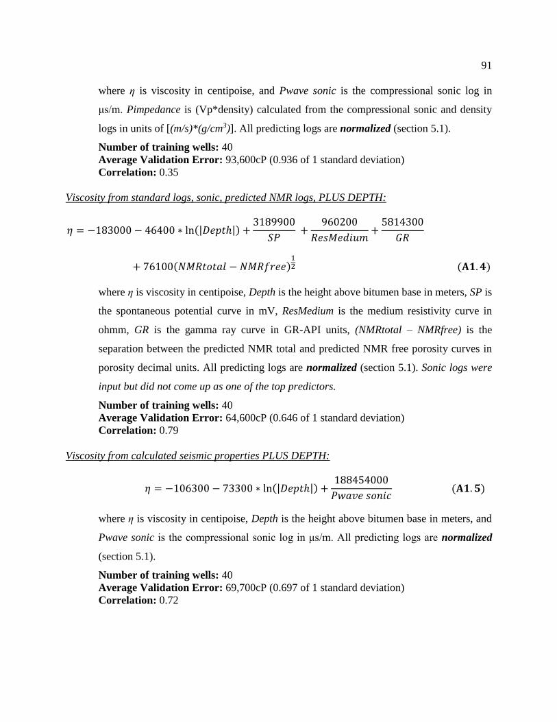
91

where η is viscosity in centipoise, and Pwave sonic is the compressional sonic log in

μs/m. Pimpedance is (Vp*density) calculated from the compressional sonic and density

logs in units of [(m/s)*(g/cm3)]. All predicting logs are normalized (section 5.1).

Number of training wells: 40

Average Validation Error: 93,600cP (0.936 of 1 standard deviation)

Correlation: 0.35

Viscosity from standard logs, sonic, predicted NMR logs, PLUS DEPTH:

𝜂 = −183000 − 46400 ∗ ln(|𝐷𝑒𝑝𝑡ℎ|) +3189900

𝑆𝑃 +

960200

𝑅𝑒𝑠𝑀𝑒𝑑𝑖𝑢𝑚+

5814300

𝐺𝑅

+ 76100(𝑁𝑀𝑅𝑡𝑜𝑡𝑎𝑙 − 𝑁𝑀𝑅𝑓𝑟𝑒𝑒)12 (𝐀𝟏. 𝟒)

where η is viscosity in centipoise, Depth is the height above bitumen base in meters, SP is

the spontaneous potential curve in mV, ResMedium is the medium resistivity curve in

ohmm, GR is the gamma ray curve in GR-API units, (NMRtotal – NMRfree) is the

separation between the predicted NMR total and predicted NMR free porosity curves in

porosity decimal units. All predicting logs are normalized (section 5.1). Sonic logs were

input but did not come up as one of the top predictors.

Number of training wells: 40

Average Validation Error: 64,600cP (0.646 of 1 standard deviation)

Correlation: 0.79

Viscosity from calculated seismic properties PLUS DEPTH:

𝜂 = −106300 − 73300 ∗ ln(|𝐷𝑒𝑝𝑡ℎ|) +188454000

𝑃𝑤𝑎𝑣𝑒 𝑠𝑜𝑛𝑖𝑐 (𝐀𝟏. 𝟓)

where η is viscosity in centipoise, Depth is the height above bitumen base in meters, and

Pwave sonic is the compressional sonic log in μs/m. All predicting logs are normalized

(section 5.1).

Number of training wells: 40

Average Validation Error: 69,700cP (0.697 of 1 standard deviation)

Correlation: 0.72

92

A.2. Other useful prediction equations not discussed in the main text

(For practical use, none of the equations in this appendix contain predicted NMR logs)

Viscosity from standard logs and sonic logs (gives very similar results to Eq. A1.1):

𝜂 = −268800 +1717200

𝑅𝑒𝑠𝑀𝑒𝑑𝑖𝑢𝑚− 146100 ∗ ln(|𝐺𝑅|) +

4219800

𝑆𝑃+

456157000

𝑃𝑤𝑎𝑣𝑒 𝑠𝑜𝑛𝑖𝑐

−311075000

𝑆𝑤𝑎𝑣𝑒 𝑠𝑜𝑛𝑖𝑐 (𝐀𝟐. 𝟏)

where η is viscosity in centipoise, ResMedium is the medium resistivity curve in ohmm,

GR is gamma ray curve in GR-API units, SP is the spontaneous potential curve in mV,

Pwave sonic and Swave sonic are the compressional and shear sonic logs in μs/m,

respectively. All predicting logs are normalized (section 5.1).

Number of training wells: 40

Average Validation Error: 71,200cP (0.712 of 1 standard deviation)

Correlation: 0.74

Viscosity from standard logs, sonic logs, PLUS DEPTH (gives very similar results to Eq. A1.4):

𝜂 = −508300 − 41400 ∗ ln(|𝐷𝑒𝑝𝑡ℎ|) +3414000

𝑆𝑃 +

954600

𝑅𝑒𝑠𝑀𝑒𝑑𝑖𝑢𝑚+

2518700

𝐺𝑅

+314070000

𝑃𝑤𝑎𝑣𝑒 𝑠𝑜𝑛𝑖𝑐−

167706000

𝑆𝑤𝑎𝑣𝑒 𝑠𝑜𝑛𝑖𝑐 (𝐀𝟐. 𝟐)

where η is viscosity in centipoise, Depth is the height above bitumen base in meters, SP is

the spontaneous potential curve in mV, ResMedium is the medium resistivity curve in

ohmm, GR is gamma ray curve in GR-API units, Pwave sonic and Swave sonic are the

compressional and shear sonic logs in μs/m, respectively. All predicting logs are

normalized (section 5.1).

Number of training wells: 40

Average Validation Error: 65,900cP (0.659 of 1 standard deviation)

Correlation: 0.78

93

Viscosity from standard logs PLUS DEPTH (extension of Eq. A1.2):

𝜂 = 99100 − 47800 ∗ ln(|𝐷𝑒𝑝𝑡ℎ|) +3452000

𝑆𝑃+

876200

𝑅𝑒𝑠𝑀𝑒𝑑𝑖𝑢𝑚+

2168300

𝐺𝑅 (𝐀𝟐. 𝟑)

where η is viscosity in centipoise, Depth is the height above bitumen base in meters, SP is

the spontaneous potential curve in mV, ResMedium is the medium resistivity curve in

ohmm, and GR is gamma ray curve in GR-API units. All predicting logs are normalized

(section 5.1).

Number of training wells: 40

Average Validation Error: 67,000cP (0.670 of 1 standard deviation)

Correlation: 0.77

A.3. Viscosity versus depth measurements from the ConocoPhillips Surmont project

Figure A3-1: Viscosity measurements plotted against reservoir depth for the

ConocoPhillips Surmont oil sands project (2015 AER presentation).