Predicting Game Level Difficulty Using Deep Neural...

IN DEGREE PROJECT COMPUTER SCIENCE AND ENGINEERING,SECOND CYCLE, 30 CREDITS

, STOCKHOLM SWEDEN 2017

Predicting Game Level Difficulty Using Deep Neural Networks

SAMI PURMONEN

KTH ROYAL INSTITUTE OF TECHNOLOGYSCHOOL OF ARCHITECTURE AND THE BUILT ENVIRONMENT

Predicting Game Level Difficulty Us-ing Deep Neural Networks

SAMI PURMONEN

Master in Computer ScienceDate: October 29, 2017Supervisor: Karl MeinkeExaminer: Olov EngwallSwedish title: Uppskattning av spelbanors svårighetsgrad med djupaneurala nätverkSchool of Computer Science and Communication

i

Abstract

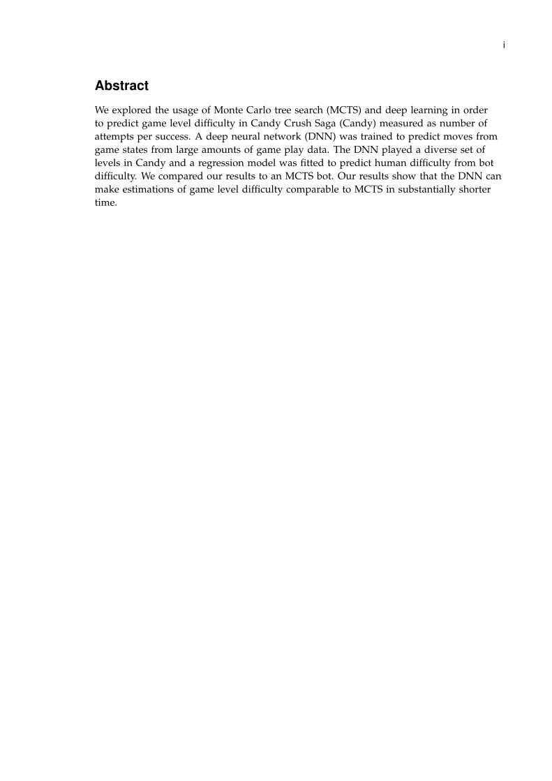
We explored the usage of Monte Carlo tree search (MCTS) and deep learning in orderto predict game level difficulty in Candy Crush Saga (Candy) measured as number ofattempts per success. A deep neural network (DNN) was trained to predict moves fromgame states from large amounts of game play data. The DNN played a diverse set oflevels in Candy and a regression model was fitted to predict human difficulty from botdifficulty. We compared our results to an MCTS bot. Our results show that the DNN canmake estimations of game level difficulty comparable to MCTS in substantially shortertime.

ii

Sammanfattning

Vi utforskade användning av Monte Carlo tree search (MCTS) och deep learning för attuppskatta banors svårighetsgrad i Candy Crush Saga (Candy). Ett deep neural network(DNN) tränades för att förutse speldrag från spelbanor från stora mängder speldata.DNN:en spelade en varierad mängd banor i Candy och en modell byggdes för att för-utse mänsklig svårighetsgrad från DNN:ens svårighetsgrad. Resultatet jämfördes medMCTS. Våra resultat indikerar att DNN:ens kan göra uppskattningar jämförbara medMCTS men på substantiellt kortare tid.

Acknowledgements

I would like to thank Prof. Karl Meinke at School of Computer Science and Communica-tion (CSC) for supervising my thesis. I would like to thank Stefan Freyr, Erik Poromaaand Alex Nodet from the AI team at King without whom this thesis work would nothave been possible. I would also like to thank John Pertoft, Philipp Eisen and Lele Caofrom the AI team at King for continuously providing feedback on my work. I would liketo thank Prof. Olov Engwall for examining my thesis.

Contents

Contents v

1 Introduction 11.1 Bot . . . . . . . . . . . . . . . . . . . . . . . . . . . . . . . . . . . . . . . . . . . 1

1.1.1 Handmade Heuristic . . . . . . . . . . . . . . . . . . . . . . . . . . . . . 11.1.2 Monte Carlo tree search . . . . . . . . . . . . . . . . . . . . . . . . . . . 21.1.3 Deep Neural Network . . . . . . . . . . . . . . . . . . . . . . . . . . . . 2

1.2 Problem . . . . . . . . . . . . . . . . . . . . . . . . . . . . . . . . . . . . . . . . 21.3 Delimitation . . . . . . . . . . . . . . . . . . . . . . . . . . . . . . . . . . . . . . 2

2 Relevant Theory 32.1 Related Work . . . . . . . . . . . . . . . . . . . . . . . . . . . . . . . . . . . . . 32.2 Monte Carlo Tree Search . . . . . . . . . . . . . . . . . . . . . . . . . . . . . . . 42.3 Machine Learning . . . . . . . . . . . . . . . . . . . . . . . . . . . . . . . . . . . 5

2.3.1 Classification . . . . . . . . . . . . . . . . . . . . . . . . . . . . . . . . . 52.3.2 Artificial Neural Network . . . . . . . . . . . . . . . . . . . . . . . . . . 62.3.3 Convolutional Neural Network . . . . . . . . . . . . . . . . . . . . . . 9

2.4 Candy Crush Saga . . . . . . . . . . . . . . . . . . . . . . . . . . . . . . . . . . 102.4.1 Basic Game Play . . . . . . . . . . . . . . . . . . . . . . . . . . . . . . . 102.4.2 Game Modes . . . . . . . . . . . . . . . . . . . . . . . . . . . . . . . . . 10

3 Method 133.1 Simplified Candy . . . . . . . . . . . . . . . . . . . . . . . . . . . . . . . . . . . 13

3.1.1 Simplified Candy . . . . . . . . . . . . . . . . . . . . . . . . . . . . . . . 133.1.2 Deterministic Greedy Bot . . . . . . . . . . . . . . . . . . . . . . . . . . 133.1.3 Generate Dataset . . . . . . . . . . . . . . . . . . . . . . . . . . . . . . . 153.1.4 Neural Network Architecture . . . . . . . . . . . . . . . . . . . . . . . . 153.1.5 Neural Network Evaluation . . . . . . . . . . . . . . . . . . . . . . . . 17

3.2 Candy . . . . . . . . . . . . . . . . . . . . . . . . . . . . . . . . . . . . . . . . . 173.2.1 Monte Carlo Tree Search . . . . . . . . . . . . . . . . . . . . . . . . . . 183.2.2 Generate Dataset . . . . . . . . . . . . . . . . . . . . . . . . . . . . . . . 183.2.3 DNN Architecture . . . . . . . . . . . . . . . . . . . . . . . . . . . . . . 203.2.4 Using DNN . . . . . . . . . . . . . . . . . . . . . . . . . . . . . . . . . . 203.2.5 Neural Network Evaluation . . . . . . . . . . . . . . . . . . . . . . . . 203.2.6 Prediction Models . . . . . . . . . . . . . . . . . . . . . . . . . . . . . . 22

3.3 Software . . . . . . . . . . . . . . . . . . . . . . . . . . . . . . . . . . . . . . . . 223.4 Hardware . . . . . . . . . . . . . . . . . . . . . . . . . . . . . . . . . . . . . . . 23

v

vi CONTENTS

4 Results 244.1 Training Neural Networks . . . . . . . . . . . . . . . . . . . . . . . . . . . . . . 244.2 Bot Performance . . . . . . . . . . . . . . . . . . . . . . . . . . . . . . . . . . . 274.3 Difficulty Predictions . . . . . . . . . . . . . . . . . . . . . . . . . . . . . . . . . 27

5 Discussion & Conclusions 295.1 Practical Usefulness . . . . . . . . . . . . . . . . . . . . . . . . . . . . . . . . . . 295.2 Method Applicability Outside Candy Crush Saga . . . . . . . . . . . . . . . . 295.3 Deep Neural Network and Monte Carlo tree search comparison . . . . . . . 295.4 Ethics of Artificial Intelligence . . . . . . . . . . . . . . . . . . . . . . . . . . . 305.5 Future Work . . . . . . . . . . . . . . . . . . . . . . . . . . . . . . . . . . . . . . 305.6 Conclusions . . . . . . . . . . . . . . . . . . . . . . . . . . . . . . . . . . . . . . 31

Bibliography 32

Chapter 1

Introduction

Playing games can be fun, but only if the game levels are not too hard nor too easy. Ifa game is too hard, players become frustrated and stop playing. If a game is too easy,players become bored and stop playing. Predicting how difficult a game level is beforereleasing it to players is difficult. In absence of any technical tools a level designer canmanually play a level many times and then make a guess of how difficult it will be forplayers in general given how difficult it was for the level designer. However, playing agame manually takes a lot of time which leads to fewer iterations before release.

It would be useful for game companies and level designers to have fast and accu-rate tools for predicting game level difficulty automatically. It is especially important forgames that continuously release new levels such as King’s Candy Crush Saga (Candy). Itwould allow level designers to tweak a level many times before release to ensure that ithas an appropriate difficulty.

1.1 Bot

One automated way of predicting game level difficulty is to create a program, a bot, thatplays the game according to some strategy. The bot can play a level many times and es-timate how difficult it is for the bot according to a difficulty measurement such as thenumbers of attempts per success. If we let the bot play many levels and estimate the botdifficulty for each of those we can compare that to how difficult those levels were for hu-mans and try to relate the bot difficulty with human difficulty. If it is the case that whena level is comparably hard for a human, it is also comparably hard for the bot, and whenit is comparably easy for a human it is comparably easy for the bot, then we might beable to create a useful regression model to predict human difficulty from bot difficulty.The difficulty of new levels can then be predicted by playing it many times with the botto measure the bot difficulty and then predicting human difficulty from bot difficulty us-ing the prediction model. There are many methods to create a strategy.

1.1.1 Handmade Heuristic

One strategy the bot can use is a handmade heuristic that ranks the available moves andthen select the best one. The heuristic can look at the current game state to judge howdesirable each available move is. The drawback of this approach is that it is not gen-eral or maintainable. When the game changes, for example a new game element is intro-

1

2 CHAPTER 1. INTRODUCTION

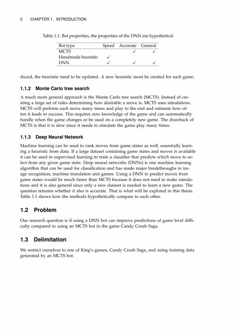
Table 1.1: Bot properties, the properties of the DNN are hypothetical

Bot type Speed Accurate GeneralMCTS X XHandmade heuristic XDNN X X X

duced, the heuristic need to be updated. A new heuristic must be created for each game.

1.1.2 Monte Carlo tree search

A much more general approach is the Monte Carlo tree search (MCTS). Instead of cre-ating a large set of rules determining how desirable a move is, MCTS uses simulations.MCTS will perform each move many times and play to the end and estimate how of-ten it leads to success. This requires zero knowledge of the game and can automaticallyhandle when the game changes or be used on a completely new game. The drawback ofMCTS is that it is slow since it needs to simulate the game play many times.

1.1.3 Deep Neural Network

Machine learning can be used to rank moves from game states as well, essentially learn-ing a heuristic from data. If a large dataset containing game states and moves is availableit can be used in supervised learning to train a classifier that predicts which move to se-lect from any given game state. Deep neural networks (DNNs) is one machine learningalgorithm that can be used for classification and has made major breakthroughs in im-age recognition, machine translation and games. Using a DNN to predict moves fromgame states would be much faster than MCTS because it does not need to make simula-tions and it is also general since only a new dataset is needed to learn a new game. Thequestion remains whether it also is accurate. That is what will be explored in this thesis.Table 1.1 shows how the methods hypothetically compare to each other.

1.2 Problem

Our research question is if using a DNN bot can improve predictions of game level diffi-culty compared to using an MCTS bot in the game Candy Crush Saga.

1.3 Delimitation

We restrict ourselves to one of King’s games, Candy Crush Saga, and using training datagenerated by an MCTS bot.

Chapter 2

Relevant Theory

In this chapter we provide the theoretical foundation that our work is based on. We takea deeper look into how neural networks work and how they are trained since it is themost important part of this thesis and where a large part of the work has been invested.

2.1 Related Work

The primary source of inspiration comes from Google Deepminds AlphaGo paper andErik Poromaas master thesis. Other sources of inspiration comes from image recognitionsince the problem of predicting moves from game states can be seen as an image recog-nition problem. Broader sources of inspiration is anything related to machine learning orAI in games.

In "Mastering the game of Go with deep neural networks and tree search" a computerGo program using a combination of supervised learning, reinforcement learning andMCTS is invented. It is the first computer Go program that could beat professional Goplayers on a full-sized board [1]. Our work is heavily inspired by the supervised learn-ing part from AlphaGo but we use it to predict game difficulty instead of creating thestrongest possible bot.

In "Crushing Candy Crush" Erik Poromaa predicts game level difficulty in CandyCrush using MCTS. He finds that this method outperforms previous state-of-the-art meth-ods of manual testing [2]. We compare our results with the MCTS bot he created.

In "ImageNet Classification with Deep Convolutional Neural Networks" a large deepconvolutional neural network is trained on millions of high-resolution images substan-tially improving previous state-of-the-art in the ImageNet LSVRC-2010 contest [3]. Eventhough the aim here is to decide what kind of object is visible in an image it is similarto our problem since the game board can be seen as an image with many more chan-nels than 3 as for RGB and the object we are trying to identify is one of the possible 144moves, therefore a convolutional neural network is suitable for our problem as well.

In "Move Evaluation in Go Using Deep Convolutional Neural Networks" a 12-layerdeep convolutional neural network is trained on a dataset of human professional Goplayers to predict moves. It predicts professional moves with 55% accuracy and couldbeat traditional search programs without any search [4]. This paper inspired AlphaGoand is very similar to what we have done in that they create a DNN bot for Go based ononly supervised learning, however we take one step further and use the bot to predictgame level difficulty.

3

4 CHAPTER 2. RELEVANT THEORY

In "Predicting moves in chess using convolutional neural networks" a deep convolu-tional neural network is trained to predict moves from game states in chess. The prob-lem with chess is that a move is defined by the position a piece is moved from and theposition it is moved to so there are 64*64 or 4096 different moves that a classifier needsto distinguish between. In order to reduce the number of moves they used a novel ap-proach of creating two separate networks, one which predicts which piece to move andone which predicts where to move it thus reducing the class space to 64 for each net-work. They managed to predict which piece to move with 38.3% accuracy [5]. Their aimto predict moves is the same as ours except we did not need to be creative in order to re-duce the class space as the number of moves in our problem is 144 which is tractable, inGo there are 361 moves.

In "Playing Atari with Deep Reinforcement Learning" a model based on convolutionalneural networks and reinforcement learning was created to play seven Atari 2600 games.It outperformed all previous approaches on six of the games and performs better than ahuman expert on three of them [6]. A similar reinforcement method would be interestingto apply on our problem but we decided to go for supervised learning instead becausewe think the best way to predict game level difficulty would be to create a bot that mim-ics human players. We could not do that since we did not have human play data at thetime this thesis was written but could do that in the future.

2.2 Monte Carlo Tree Search

It is common to use different game tree search algorithms when creating agents playinggames. The Minimax algorithm is a tree search algorithm that has reached state-of-the-art performance in games such as Chess, Checkers and Othello where good heuristics forevaluating game states are available [1]. In games such as Go where it is hard to comeup with heuristics, MCTS has instead been the most successful game search algorithmuntil AlphaGo [4].

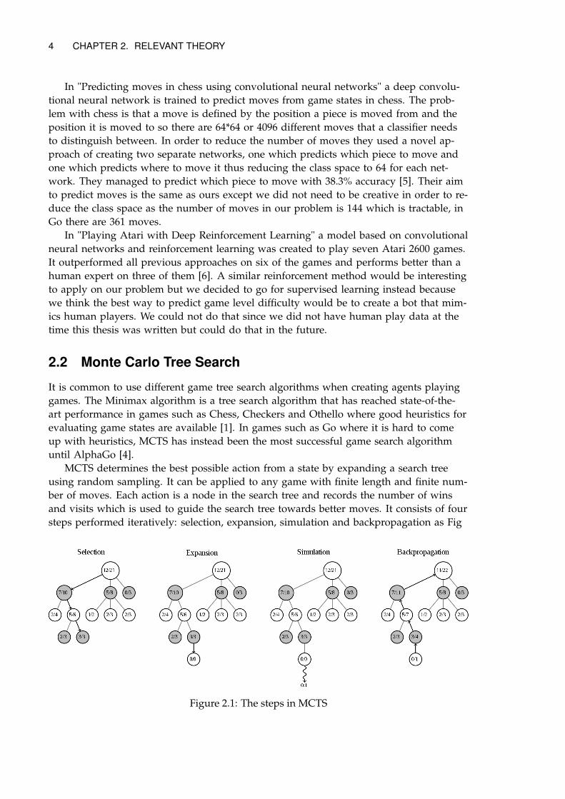
MCTS determines the best possible action from a state by expanding a search treeusing random sampling. It can be applied to any game with finite length and finite num-ber of moves. Each action is a node in the search tree and records the number of winsand visits which is used to guide the search tree towards better moves. It consists of foursteps performed iteratively: selection, expansion, simulation and backpropagation as Fig

Figure 2.1: The steps in MCTS

CHAPTER 2. RELEVANT THEORY 5

2.1. Doing this many times converges to optimal play [7].

Selection

The selection starts at current state which is the root of the search tree then it selectschild nodes until it reaches a leaf node. The selection of child nodes is done in a waythat will expand the tree towards the most promising move using the number of winsand visits but also allows exploration.

Expansion

When a leaf node is reached, the search tree is expanded with a new child node unlessthe game has reached the end.

Simulation

The game is simulated to the end by randomly selecting actions.

Backpropagation

The result of the playout is backpropagated through all visited nodes back to the rootupdating the number of wins and visits.

2.3 Machine Learning

Machine learning encompasses algorithms that learn from experience. Supervised learn-ing is the most common form of machine learning. A supervised learning algorithmlearn a function F : RN → RM from a training set of examples of such mappings andthen its predictions on unseen data becomes better, meaning that it is generalizing.

2.3.1 Classification

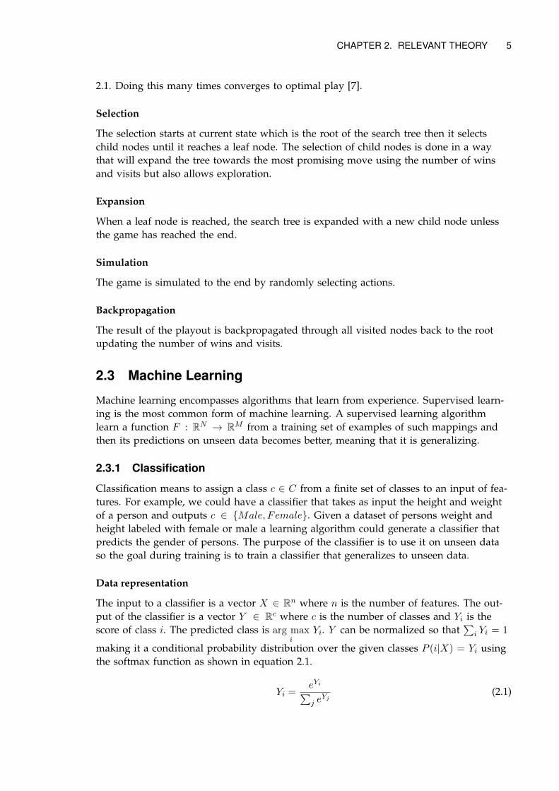
Classification means to assign a class c ∈ C from a finite set of classes to an input of fea-tures. For example, we could have a classifier that takes as input the height and weightof a person and outputs c ∈ {Male, Female}. Given a dataset of persons weight andheight labeled with female or male a learning algorithm could generate a classifier thatpredicts the gender of persons. The purpose of the classifier is to use it on unseen dataso the goal during training is to train a classifier that generalizes to unseen data.

Data representation

The input to a classifier is a vector X ∈ Rn where n is the number of features. The out-put of the classifier is a vector Y ∈ Rc where c is the number of classes and Yi is thescore of class i. The predicted class is arg max

iYi. Y can be normalized so that

∑i Yi = 1

making it a conditional probability distribution over the given classes P (i|X) = Yi usingthe softmax function as shown in equation 2.1.

Yi =eYi∑j e

Yj(2.1)


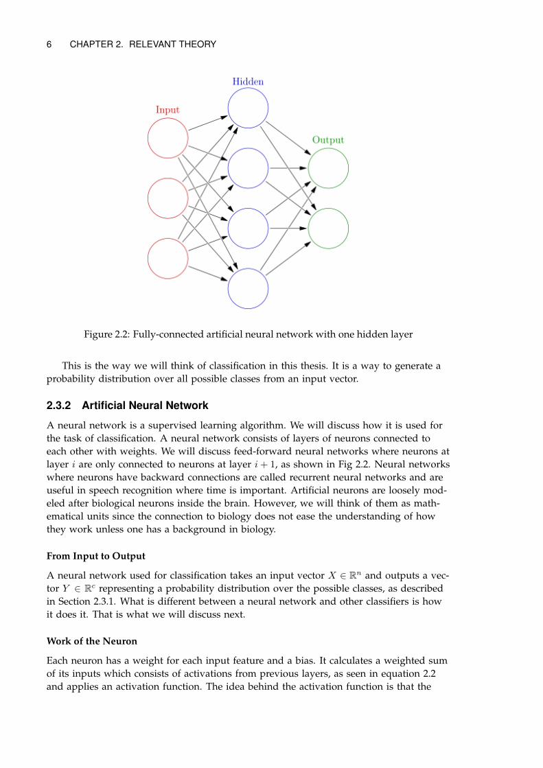
Figure 2.2: Fully-connected artificial neural network with one hidden layer

This is the way we will think of classification in this thesis. It is a way to generate aprobability distribution over all possible classes from an input vector.

2.3.2 Artificial Neural Network

A neural network is a supervised learning algorithm. We will discuss how it is used forthe task of classification. A neural network consists of layers of neurons connected toeach other with weights. We will discuss feed-forward neural networks where neurons atlayer i are only connected to neurons at layer i+ 1, as shown in Fig 2.2. Neural networkswhere neurons have backward connections are called recurrent neural networks and areuseful in speech recognition where time is important. Artificial neurons are loosely mod-eled after biological neurons inside the brain. However, we will think of them as math-ematical units since the connection to biology does not ease the understanding of howthey work unless one has a background in biology.

From Input to Output

A neural network used for classification takes an input vector X ∈ Rn and outputs a vec-tor Y ∈ Rc representing a probability distribution over the possible classes, as describedin Section 2.3.1. What is different between a neural network and other classifiers is howit does it. That is what we will discuss next.

Work of the Neuron

Each neuron has a weight for each input feature and a bias. It calculates a weighted sumof its inputs which consists of activations from previous layers, as seen in equation 2.2and applies an activation function. The idea behind the activation function is that the


neuron has a binary output, it either fires or not. Each neuron detects patterns in the in-puts from previous layers and fires when it sees it. It also introduces non-linearity in thenetwork which is necessary to be able to approximate non-linear functions.

Aj = g((∑i

WjiXi) + bj) (2.2)

A common activation function is the sigmoid as seen in equation 2.3.

sigmoid(x) =1

1 + e−x(2.3)

Another common activation function is TanH.

tanh(x) =2

1 + e−2x− 1 (2.4)

Backpropagation uses the gradients of the cost function to update the weights of theneural network so there is a problem if the gradients become very small as that makesthe updates small and learning slow. Both the sigmoid and tanh have a problem with di-minishing gradients as they map inputs to a small range. The rectified linear unit shownin Eq. 2.5 is another activation function that has less problems with diminishing gradi-ents as it only truncates negative values to zero. It is several times faster to train becauseit is non-saturating meaning that outputs are not bounded upwards and can become ar-bitrarily large [3]. It is currently the most popular activation function used in deep learn-ing [8].

ReLU(x) = max(x, 0) (2.5)

The rectified linear unit has a problem when the input becomes truncated to zero asthat makes the gradients zero and no learning is possible. The exponential linear unit(ELU) seen in Eq. 2.6 was introduced to handle this problem by allowing negative values[9]. It is however more computationally expensive than the ReLU.

ELU(x) =

{x, for x ≥ 0

α(ex − 1), for x ≤ 0

}(2.6)

Cost Function

In order to improve the neural network there must be an objective measurement of howgood or bad the network performs. This is captured with a cost function. If the networksoutput is close to the desired output, the cost is low, otherwise it is high. A commonlyused cost function is mean square error as shown in equation 2.7.

C =1

2(f(x)− y)2 (2.7)

Another commonly used cost function is cross entropy which has significant practicaladvantages as better local optimums can be found when weights are randomly initialized[10, 11]. Using cross entropy cost function instead of mean square error together with thesoftmax activation function leads to more accurate results [12].

C = −∑c

yc log f(x)c + (1− yc) log (1− f(x)c) (2.8)


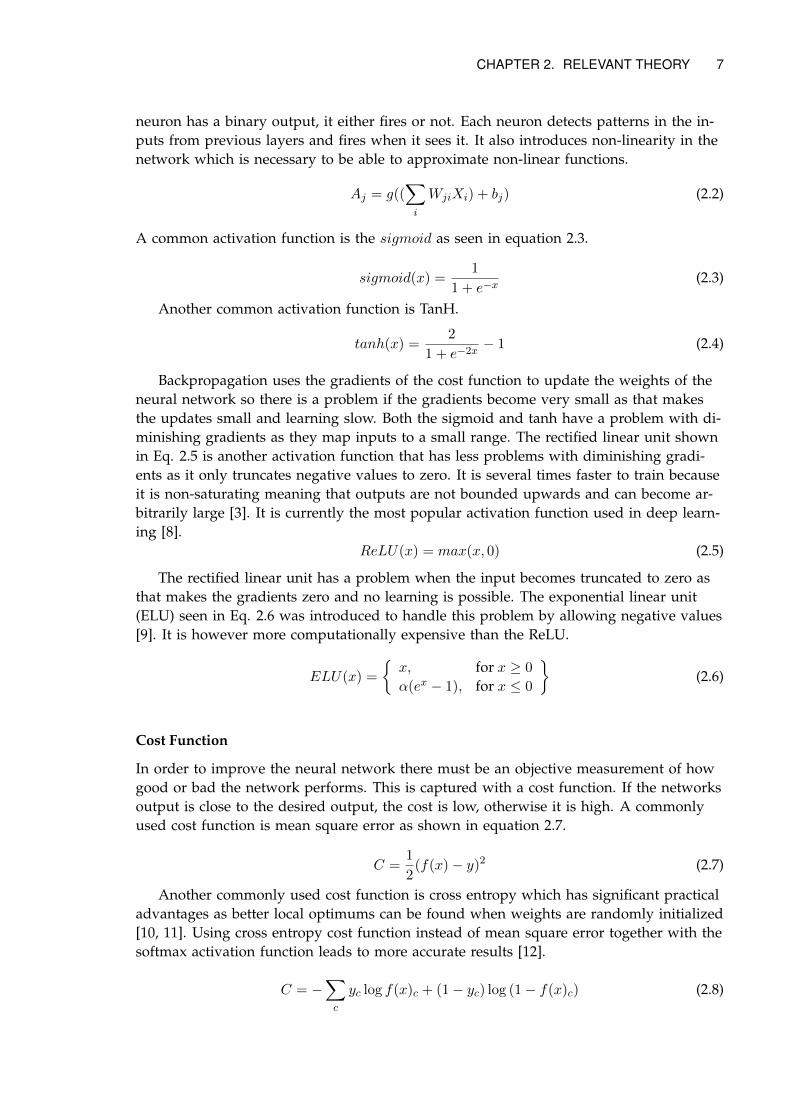
(a) Sigmoid function (b) TanH function

(c) ReLU function (d) ELU function

Figure 2.3: Activation functions

Learning

The network learns by calculating the cost function and updating its weights in orderto minimize the cost function. The learning process is thus an optimization problem.The cost function is a function of the weights. In order to minimize it gradient descentis used. Gradient descent calculates the gradient of the cost function with respect to tothe weights. It then updates the weights in the opposite direction as to make the costsmaller as seen in 2.9. How big the weight differences are is decided by the learning rate.In practice gradient descent is not feasible with large amounts of data so instead stochas-tic gradient descent is used where only a small subset of the training data is used to cal-culate an estimate of the cost function which makes the training time faster [13].

wi = wi − λ∂C

∂wi(2.9)

Hyper Parameters

When a neural network is trained it learns what weights it should have. Parameters thataffect the training such as the network architecture but are not learned during trainingare called hyperparameters. A neural network has a lot of hyperparameters.

• Learning rate

• Number of hidden layers

• Number of hidden nodes

• Choice of activation function

• Choice of error measurement

• Learning rate decay

• Regularization


• Initial weights

These can be decided by manually testing different combinations. A more rigorous wayto choose them is a grid search or random search. In a grid search a finite set of val-ues for each parameter is chosen then all combinations are tried. The one yielding thehighest accuracy is selected as the best parameter combination. A random search selectsparameters randomly which has shown to be more efficient than grid search [14]. Ge-netic algorithms breeding new combinations by combining previous successful combi-nations can also be applied. A novel approach based on reinforcement learning for gen-erating architectures using the validation accuracy on the validation set as feedback hasbeen demonstrated to be capable of generating architectures that rivals the best human-invented architectures on the CIFAR-10 dataset [15].

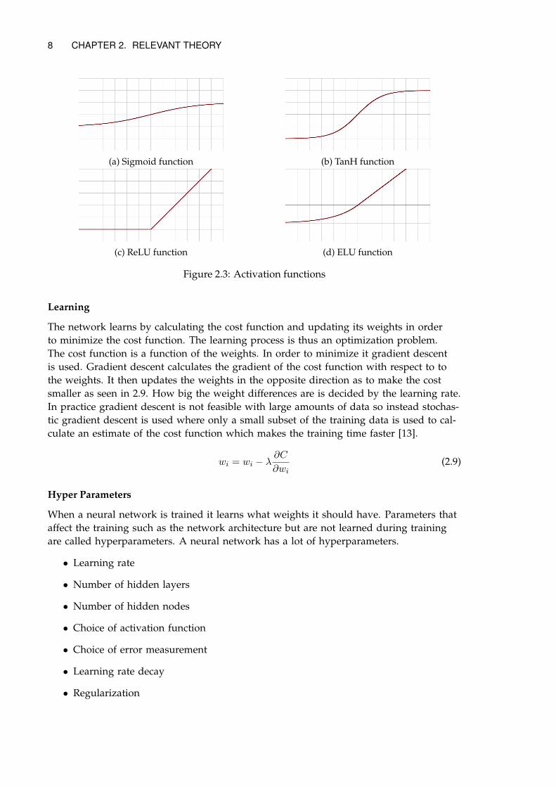
2.3.3 Convolutional Neural Network

Convolutional neural networks (CNN) have dramatically improved object recognitionand is the current state-of-the-art for this task [16]. In a CNN each neuron is connectedin overlapping tiles giving the network locality in a two-dimensional space. This workswell for input data that can be treated as images or grids [16].

Input

Instead of treating input data as a 1-dimensional vector it is treated as 3-dimensionalvector. An rgb image of size 9 × 9 would have dimensions 9 × 9 × 3 since it has 3 colorchannels.

Patch Size

The patch size determines how large area a neuron covers. A 3 × 3 patch is the mostcommon size and means that each neuron in layer i + 1 is connected to a 3 × 3 tile ofneurons in layer i.

Stride

The stride determines the distance between each input to the filter.

Filter

The number of filters determines how many features can be detected in each layer sincethe filters share weights.

Pooling

Pooling means reducing the dimensions of the input by summarizing its inputs. A 2 × 2

max pooling for example would take an input of 2 × 2 and output 1 × 1 with the highestvalue found in the input and stride over data.


2.4 Candy Crush Saga

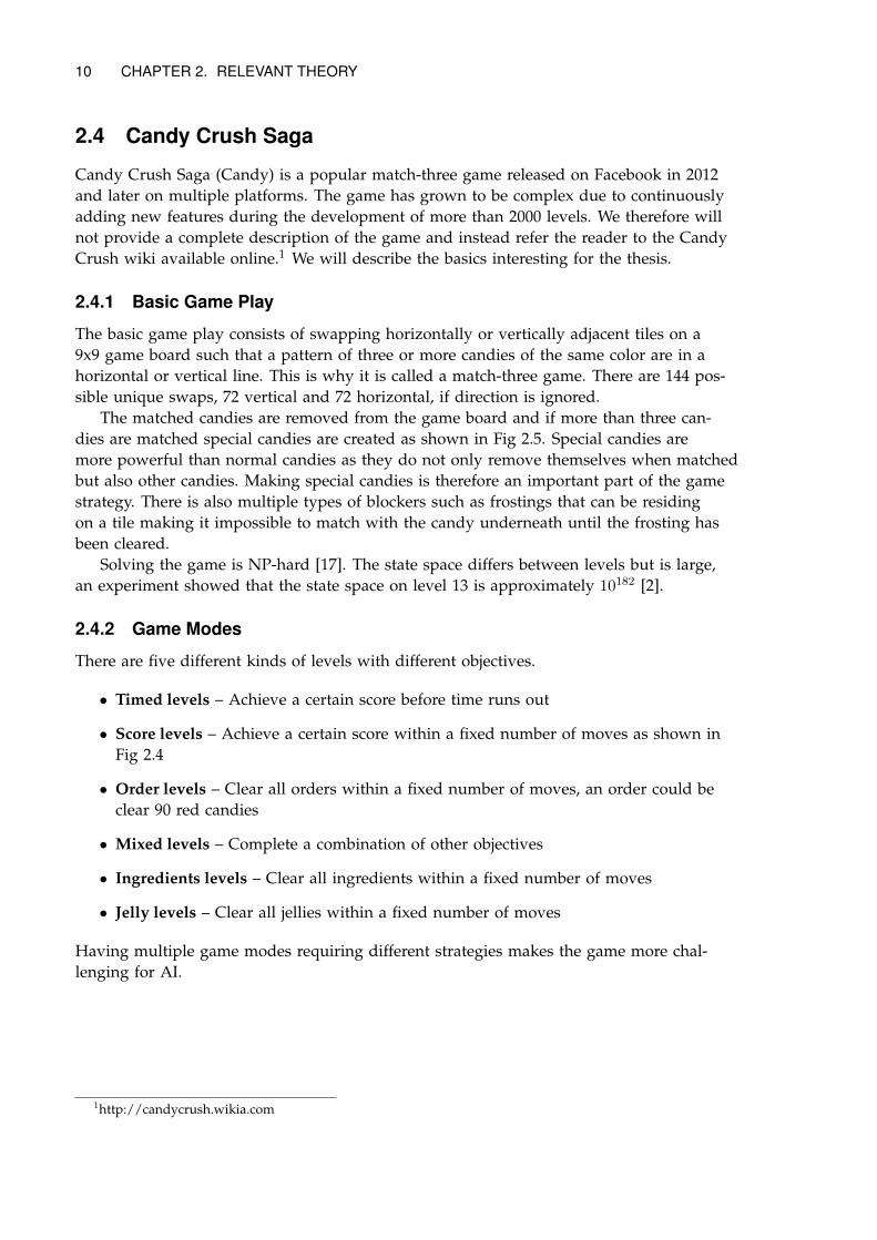
Candy Crush Saga (Candy) is a popular match-three game released on Facebook in 2012and later on multiple platforms. The game has grown to be complex due to continuouslyadding new features during the development of more than 2000 levels. We therefore willnot provide a complete description of the game and instead refer the reader to the CandyCrush wiki available online.1 We will describe the basics interesting for the thesis.

2.4.1 Basic Game Play

The basic game play consists of swapping horizontally or vertically adjacent tiles on a9x9 game board such that a pattern of three or more candies of the same color are in ahorizontal or vertical line. This is why it is called a match-three game. There are 144 pos-sible unique swaps, 72 vertical and 72 horizontal, if direction is ignored.

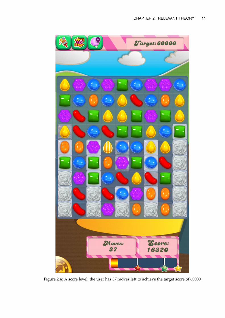
The matched candies are removed from the game board and if more than three can-dies are matched special candies are created as shown in Fig 2.5. Special candies aremore powerful than normal candies as they do not only remove themselves when matchedbut also other candies. Making special candies is therefore an important part of the gamestrategy. There is also multiple types of blockers such as frostings that can be residingon a tile making it impossible to match with the candy underneath until the frosting hasbeen cleared.

Solving the game is NP-hard [17]. The state space differs between levels but is large,an experiment showed that the state space on level 13 is approximately 10182 [2].

2.4.2 Game Modes

There are five different kinds of levels with different objectives.

• Timed levels – Achieve a certain score before time runs out

• Score levels – Achieve a certain score within a fixed number of moves as shown inFig 2.4

• Order levels – Clear all orders within a fixed number of moves, an order could beclear 90 red candies

• Mixed levels – Complete a combination of other objectives

• Ingredients levels – Clear all ingredients within a fixed number of moves

• Jelly levels – Clear all jellies within a fixed number of moves

Having multiple game modes requiring different strategies makes the game more chal-lenging for AI.

1http://candycrush.wikia.com


Figure 2.4: A score level, the user has 37 moves left to achieve the target score of 60000


Figure 2.5: Three different swaps, the leftmost creates a color bomb, the center creates ahorizontal striped candy, the rightmost creates no special candy

Chapter 3

Method

In this chapter we give a detailed description of our method. It is divided into two parts,experiments on a simplified version of Candy and experiments on Candy.

3.1 Simplified Candy

When the thesis started we did not yet have training data available from Candy and wewanted to explore deep learning on a simplified problem to get a notion of how power-ful and suitable it is for our space of problems. Therefore we decided to:

1. Build a simplified version of Candy

2. Create a deterministic greedy bot

3. Generate dataset from the greedy bot playing Candy

4. Train a DNN

5. Evaluate classification performance

Since we do not have any human difficulty data for simplified Candy we do not at-tempt to predict difficulty for this experiment. We only explore the classification task.

3.1.1 Simplified Candy

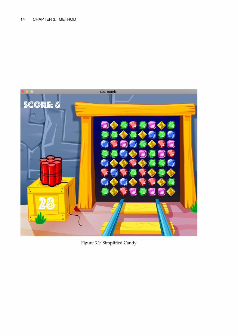
Simplified Candy was implemented in C++ and can be played with or without a GUI.It can be seen in Fig 3.1. It has a slightly smaller game board of 8 × 8 compared to thereal game which has 9 × 9. It has 5 different candy colors instead of 6. It has no specialcandies or blockers. It has no objectives. The game automatically stops after a 60 secondsand the score increases proportionally to the number of candies cleared. New candies aregenerated randomly from a uniform distribution.

3.1.2 Deterministic Greedy Bot

We created a deterministic greedy bot that always selects the move which clears the mostcandies. It will always prefer a five-match to a four-match and a four-match to a three-match. If there are multiple moves that clears equally many candies, it prefers horizontalswaps to vertical swaps and north-west positions to south-east positions. This makes the

13

14 CHAPTER 3. METHOD

Figure 3.1: Simplified Candy

CHAPTER 3. METHOD 15

2 0 1 4 3 0 0 11 4 0 3 2 2 3 44 1 2 2 3 1 4 11 3 0 1 4 2 0 31 0 3 0 1 3 1 32 2 4 0 4 1 1 44 3 0 3 0 4 2 12 1 1 4 1 2 4 4

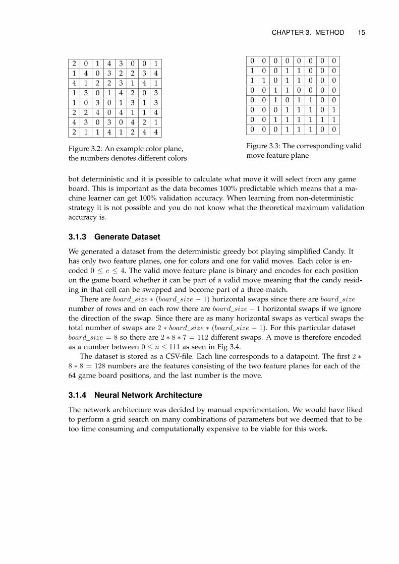
Figure 3.2: An example color plane,the numbers denotes different colors

0 0 0 0 0 0 0 01 0 0 1 1 0 0 01 1 0 1 1 0 0 00 0 1 1 0 0 0 00 0 1 0 1 1 0 00 0 0 1 1 1 0 10 0 1 1 1 1 1 10 0 0 1 1 1 0 0

Figure 3.3: The corresponding validmove feature plane

bot deterministic and it is possible to calculate what move it will select from any gameboard. This is important as the data becomes 100% predictable which means that a ma-chine learner can get 100% validation accuracy. When learning from non-deterministicstrategy it is not possible and you do not know what the theoretical maximum validationaccuracy is.

3.1.3 Generate Dataset

We generated a dataset from the deterministic greedy bot playing simplified Candy. Ithas only two feature planes, one for colors and one for valid moves. Each color is en-coded 0 ≤ c ≤ 4. The valid move feature plane is binary and encodes for each positionon the game board whether it can be part of a valid move meaning that the candy resid-ing in that cell can be swapped and become part of a three-match.

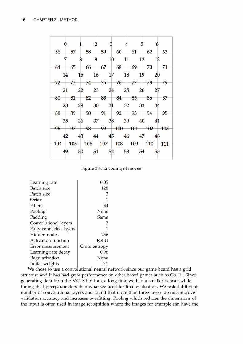
There are board_size ∗ (board_size − 1) horizontal swaps since there are board_sizenumber of rows and on each row there are board_size − 1 horizontal swaps if we ignorethe direction of the swap. Since there are as many horizontal swaps as vertical swaps thetotal number of swaps are 2 ∗ board_size ∗ (board_size − 1). For this particular datasetboard_size = 8 so there are 2 ∗ 8 ∗ 7 = 112 different swaps. A move is therefore encodedas a number between 0 ≤ n ≤ 111 as seen in Fig 3.4.

The dataset is stored as a CSV-file. Each line corresponds to a datapoint. The first 2 ∗8 ∗ 8 = 128 numbers are the features consisting of the two feature planes for each of the64 game board positions, and the last number is the move.

3.1.4 Neural Network Architecture

The network architecture was decided by manual experimentation. We would have likedto perform a grid search on many combinations of parameters but we deemed that to betoo time consuming and computationally expensive to be viable for this work.


Figure 3.4: Encoding of moves

Learning rate 0.05Batch size 128Patch size 3Stride 1Filters 34Pooling NonePadding SameConvolutional layers 3Fully-connected layers 1Hidden nodes 256Activation function ReLUError measurement Cross entropyLearning rate decay 0.96Regularization NoneInitial weights 0.1

We chose to use a convolutional neural network since our game board has a gridstructure and it has had great performance on other board games such as Go [1]. Sincegenerating data from the MCTS bot took a long time we had a smaller dataset whiletuning the hyperparameters than what we used for final evaluation. We tested differentnumber of convolutional layers and found that more than three layers do not improvevalidation accuracy and increases overfitting. Pooling which reduces the dimensions ofthe input is often used in image recognition where the images for example can have the


size 256x256. We chose not to use pooling since our 9x9 game board already is small.

3.1.5 Neural Network Evaluation

The dataset was divided into a training set and a validation set. The training set is usedduring training to update the weights of the network. The validation set is used for eval-uation. The performance measured used during training is validation accuracy as seen inequation 3.1. We also calculated validation top 2 accuracy and validation top 3 accuracymeaning how often the correct move was found in the top 2 and top 3 moves.

correct

total(3.1)

The validation accuracy is not a perfect measurement of game strategy since the se-lected action in a game state is non-deterministic, meaning that a player in certain gamestate multiple times may choose different actions. If a player is in a state with 10 legalactions and the player selects one out of two actions with 50% probability then the theo-retical maximum validation accuracy would be 50%, but if the network learned the cor-rect probability distribution it would have perfectly learned the game strategy. The idealwould be to use a measurement between the distance of the real and predicted probabil-ity distributions rather than validation accuracy such as the Kullback–Leibler divergenceshown in equation 3.2.

∑i

P (i) lnP (i)

Q(i)(3.2)

However, since the state space is so large it is very rare that there are multiple train-ing samples from a specific state making it impossible to estimate a probability distribu-tion in the specific state. Validation accuracy is therefore chosen for pragmatic reasons.

Having no other benchmarks this is compared to the expected accuracy of randomlyselecting moves in each game state calculated as shown in equation 3.3 where Si is thenumber of moves available in state i.

1

n

n∑i

1

Si(3.3)

3.2 Candy

The experiment on Candy consists of the following steps.

1. Generate dataset from an MCTS bot playing Candy

2. Train a DNN

3. Play different Candy levels with different bots using DNN and MCTS

4. Evaluate performance measured as cumulative success rate and mean success rate

5. Create a regression models to predict human difficulty from bot difficulty measuredas attempts per success


Just as for simplified Candy we generate training data and then train a neural net-work but then we proceed to use the neural network to actually play the game and mea-sure the bots performance in terms of success rate and create a model to predict humandifficulty from bot difficulty measured as attempts per success.

3.2.1 Monte Carlo Tree Search

MCTS algorithm used was provided by King. It is written in C++ on top of the Candysource code. The implementation has a few novelties. Instead of only using win or lossas the signal a continuous signal is used based on partial goals such as the number ofjellies cleared and/or the score. We treat it as a black box that can be configured to use atrained DNN during playouts hence a more detailed description is not necessary but isavailable in Erik Poromaas master thesis [2].

3.2.2 Generate Dataset

Since we want to use the neural network to predict difficulty for players it would makemost sense to use game play data from players. However, that data was not availableand we could not get it for the thesis. We did have an MCTS bot that could play thegame very well. We let the MCTS bot using 1000 simulations per move play a diverseset of levels between level 1000 and level 2000 and added logging of all (state, action)pairs during game play in a CSV-format directly usable for training a neural network.We gathered close to 2 million data points. 50k data points was used for validation andthe rest was used for training.

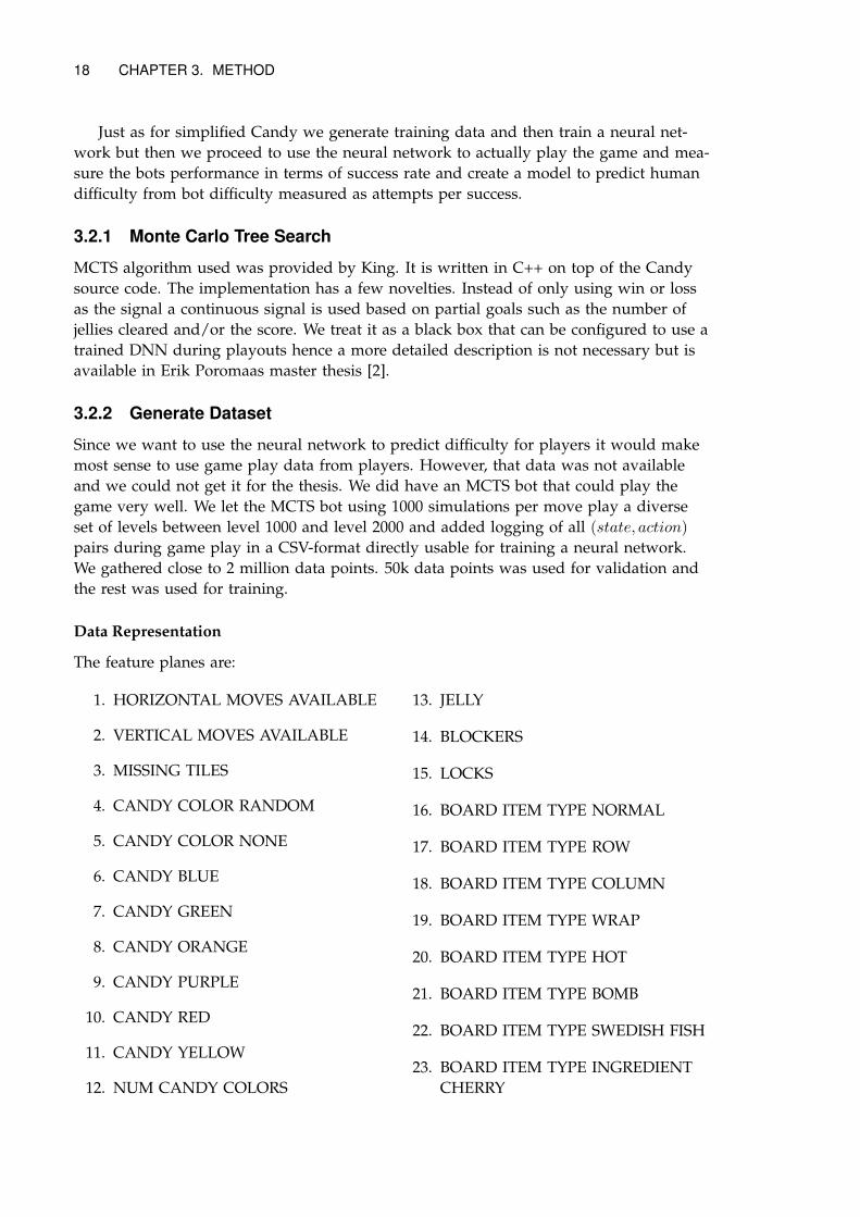
Data Representation

The feature planes are:

1. HORIZONTAL MOVES AVAILABLE

2. VERTICAL MOVES AVAILABLE

3. MISSING TILES

4. CANDY COLOR RANDOM

5. CANDY COLOR NONE

6. CANDY BLUE

7. CANDY GREEN

8. CANDY ORANGE

9. CANDY PURPLE

10. CANDY RED

11. CANDY YELLOW

12. NUM CANDY COLORS

13. JELLY

14. BLOCKERS

15. LOCKS

16. BOARD ITEM TYPE NORMAL

17. BOARD ITEM TYPE ROW

18. BOARD ITEM TYPE COLUMN

19. BOARD ITEM TYPE WRAP

20. BOARD ITEM TYPE HOT

21. BOARD ITEM TYPE BOMB

22. BOARD ITEM TYPE SWEDISH FISH

23. BOARD ITEM TYPE INGREDIENTCHERRY


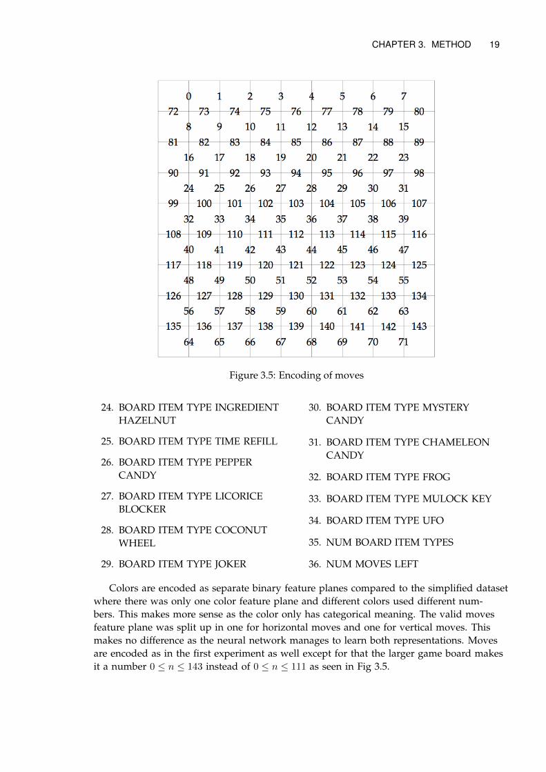
Figure 3.5: Encoding of moves

24. BOARD ITEM TYPE INGREDIENTHAZELNUT

25. BOARD ITEM TYPE TIME REFILL

26. BOARD ITEM TYPE PEPPERCANDY

27. BOARD ITEM TYPE LICORICEBLOCKER

28. BOARD ITEM TYPE COCONUTWHEEL

29. BOARD ITEM TYPE JOKER

30. BOARD ITEM TYPE MYSTERYCANDY

31. BOARD ITEM TYPE CHAMELEONCANDY

32. BOARD ITEM TYPE FROG

33. BOARD ITEM TYPE MULOCK KEY

34. BOARD ITEM TYPE UFO

35. NUM BOARD ITEM TYPES

36. NUM MOVES LEFT

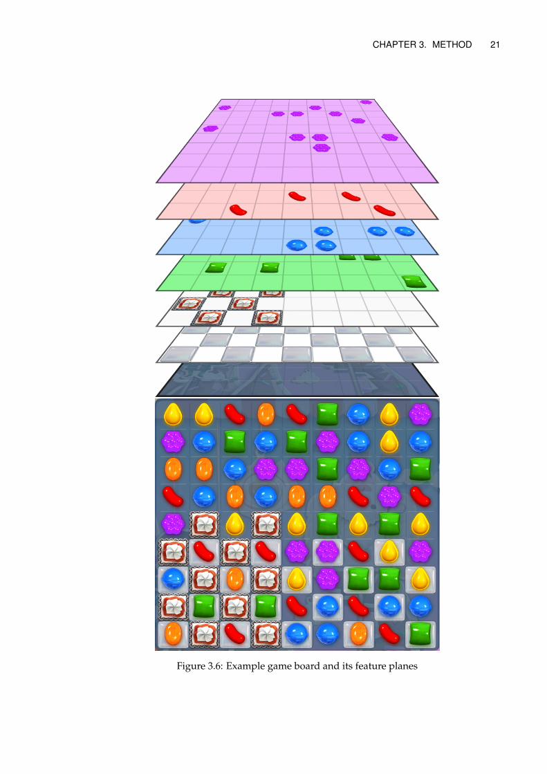
Colors are encoded as separate binary feature planes compared to the simplified datasetwhere there was only one color feature plane and different colors used different num-bers. This makes more sense as the color only has categorical meaning. The valid movesfeature plane was split up in one for horizontal moves and one for vertical moves. Thismakes no difference as the neural network manages to learn both representations. Movesare encoded as in the first experiment as well except for that the larger game board makesit a number 0 ≤ n ≤ 143 instead of 0 ≤ n ≤ 111 as seen in Fig 3.5.


Drawbacks

While direction of the move does not matter in the simplified Candy, it does matter inCandy. When matching two special candies the impact on the game board will be dif-ferent depending on direction. In order to capture this we would need to distinguish be-tween 288 moves instead of 144. This may make it impossible to learn advanced strate-gies where certain combinations of special candies and directions are necessary to clearthe level. However, we do note that we have a 50% chance of making the swap in thebest direction and that having two adjacent striped candies is not a common situationso we decided to discard the direction as having twice as many classes would make itharder to train the DNN.

There are a few other drawbacks with the dataset. The biggest one is that there is nofeature plane for the goal of the level. If the goal is clearing jellies the data does not con-tain the number of jellies to be cleared or if the goal is to clear ingredients there is nofeature plane containing the number ingredients left to be cleared. This will likely makeit harder for the network to learn to prioritize the goal when the number of moves leftare few rather than creating fancy special candies.

3.2.3 DNN Architecture

We used the same DNN as for simple Candy.

3.2.4 Using DNN

The DNN was used through an HTTP server written in Python because we deemed it tocumbersome to embed it inside the MCTS C++ source code using the immature Tensor-Flow C++ API. Having the HTTP server running on the same physical machine as thebot made the networking overhead insignificant.

We tested to let the DNN play by itself and during MCTS playouts. The highest prob-able move according to the DNN was selected.

3.2.5 Neural Network Evaluation

Training is evaluated the same as for simple Candy. We used in total 4 bots for compar-isons. The bots are also compared to human players. We compare the cumulative suc-cess rates of the bots to measure their performance. We also fit models to predict humanattempts per success from the bots attempts per success in order to measure their pre-dictive power. MCTS performs 100 attempts per level and DNN performs both 100 and1000 attempts per level because it is much faster.

Random Bot

The random bot selects moves randomly from a uniform distribution. It is the defaultbaseline.

DNN Bot

The DNN bot selects the most probable move according to the deep neural network. Itdoes not do any search.


Figure 3.6: Example game board and its feature planes


MCTS + Random Bot

The MCTS + Random bot uses MCTS with random playouts. It serves as a baseline forMCTS + DNN bot.

MCTS + DNN Bot

The MCTS + DNN bot uses MCTS with DNN during playouts where the highest proba-ble move according to the DNN was selected.

3.2.6 Prediction Models

We played 361 levels with the bots to calculate the bot difficulty measured as attemptsper success. We let each bot make 100 attempts on each level except for the DNN whichwe allowed to make 1000 attempts because it is much faster. Player data was availablefor those levels so we could also calculate human attempts per success. Bot difficulty isnot the same as human difficulty but they are correlated. We fit a regression model topredict human attempts per success from bots attempts per success. We use mean abso-lute error as a measure of predictive accuracy which intuitively means how wrong thepredictions were on average.

We divide the levels into three groups, green, yellow and red depending on how hardthey are for each because we saw that the relationship between human attempts per suc-cess and bot attempts per success differed for easier levels and harder levels. We fit aseparate prediction model for each group for each bot. The green levels have an attemptsper success lower than or equal to a preselected cutoff. The yellow levels have a higherattempts per success than the cutoff. Red levels have zero successes so attempts per suc-cess is undefined. We used the mean of human attempts per success as predicted valuefor red levels.

3.3 Software

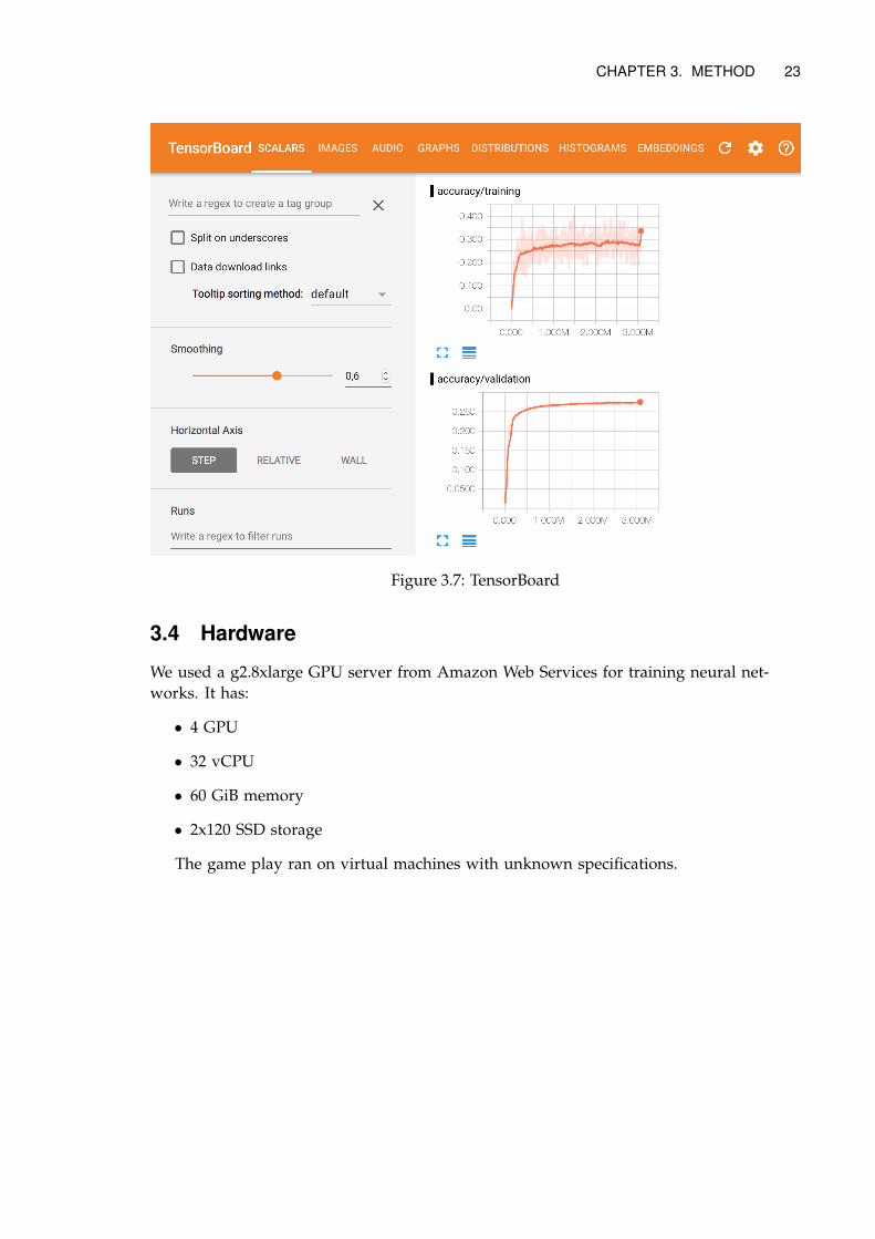
We used the deep learning library TensorFlow to implement the DNN. Google createdTensorFlow to replace DistBelief which is widely used within Google [18]. TensorFlow iswritten in C++ with an API available in Python. It is not as fast as other deep learning li-braries available such as Torch and Theano [19], but comes with many helpful tools. Ten-sorBoard is a web interface that visualizes training. When creating a TensorFlow graphit is possible to add nodes for logging measurements such as validation accuracy, crossentropy and learning rate. TensorBoard can display the logged measurements in graphsdynamically created during training as seen in Fig 3.7.


Figure 3.7: TensorBoard

3.4 Hardware

We used a g2.8xlarge GPU server from Amazon Web Services for training neural net-works. It has:

• 4 GPU

• 32 vCPU

• 60 GiB memory

• 2x120 SSD storage

The game play ran on virtual machines with unknown specifications.

Chapter 4

Results

4.1 Training Neural Networks

This part shows the performance of the DNN during training. The validation accuracyshows how the DNN is expected to perform on unseen data. We also include how of-ten the correct move was in the top 2 and top 3. The end result of training and detailsof datasets used is shown in Table 4.1. Plots of validation accuracies during training isshown in Fig 4.1 and Fig 4.2.

The validation accuracy on the simplified dataset is high and reaches 92.2% as seenin Table 4.1. Given more data, more training time and a bigger model it would likely beable to become even better. Perhaps close to 100%.

The validation accuracy on the MCTS data is much lower at 28.3%. This is not sur-prising as it is generated from a non-deterministic algorithm. 28.3% is still a lot higherthan 16.3% which random guessing would give. Given that we do not know how pre-dictable the MCTS data is it is hard to know how good our network has been on learn-ing it. It could be that 30% is the theoretical maximum validation accuracy, in which case28.3% is good, or it could be much higher, in which case 28.3% might be pretty bad. Inorder to get an understanding of how well the DNN has learned to play like MCTS weneed to play the game with the DNN and compare its performance with MCTS. We dothat in the next section.

The training accuracy jumps up and down a lot in the graphs. That is because it iscalculated on a small randomly selected batch of 128 datapoints. The training accuracyappears to be close to the validation accuracy for both datasets. This implies that theneural network has not overfitted which suggests that there is room for increasing themodel size. We would have done that but ran out of time. During the thesis work wecontinuously collected more data and the DNN overfitted until the last dataset whichwas large enough to make it not overfit.

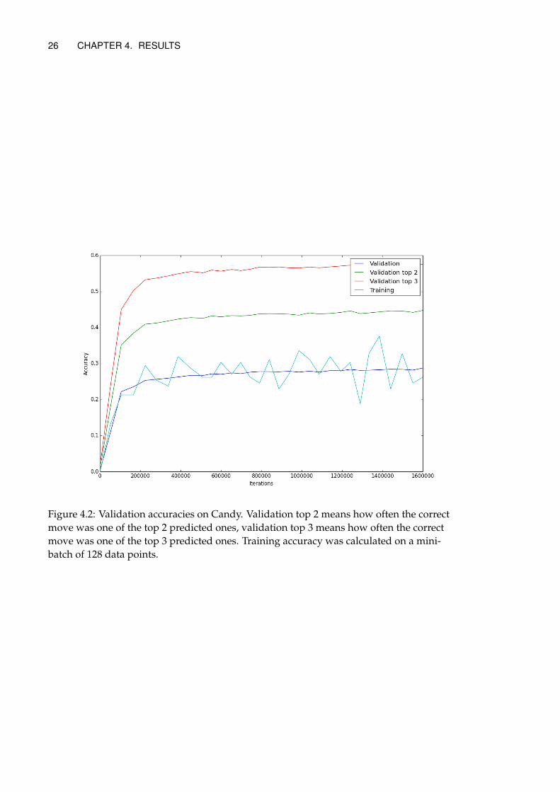
Looking at validation, validation top-2 and validation top-3 accuracies we note thatthe DNN trained on MCTS data improves from 28.3% to 44.4% to 57.3%. This impliesthat even when it fails to select the correct move the correct move is often in the top-3.Considering that there are many situations in Candy where multiple moves appear to beequally good it is not surprising if it is hard to distinguish between them.

24

CHAPTER 4. RESULTS 25

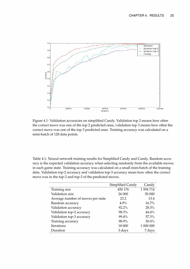
Figure 4.1: Validation accuracies on simplified Candy. Validation top 2 means how oftenthe correct move was one of the top 2 predicted ones, validation top 3 means how often thecorrect move was one of the top 3 predicted ones. Training accuracy was calculated on amini-batch of 128 data points.

Table 4.1: Neural network training results for Simplified Candy and Candy. Random accu-racy is the expected validation accuracy when selecting randomly from the available movesin each game state. Training accuracy was calculated on a small mini-batch of the trainingdata. Validation top-2 accuracy and validation top-3 accuracy mean how often the correctmove was in the top-2 and top-3 of the predicted moves.

Simplified Candy CandyTraining size 450 176 1 594 714Validation size 26 000 50 000Average number of moves per state 23.2 13.4Random accuracy 4.9% 16.7%Validation accuracy 92.2% 28.3%Validation top-2 accuracy 98.3% 44.4%Validation top-3 accuracy 99.4% 57.3%Training accuracy 98.9% 30.4%Iterations 18 000 1 000 000Duration 3 days 7 days

26 CHAPTER 4. RESULTS

Figure 4.2: Validation accuracies on Candy. Validation top 2 means how often the correctmove was one of the top 2 predicted ones, validation top 3 means how often the correctmove was one of the top 3 predicted ones. Training accuracy was calculated on a mini-batch of 128 data points.

CHAPTER 4. RESULTS 27

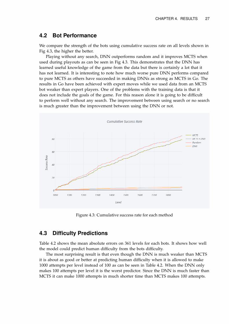
4.2 Bot Performance

We compare the strength of the bots using cumulative success rate on all levels shown inFig 4.3, the higher the better.

Playing without any search, DNN outperforms random and it improves MCTS whenused during playouts as can be seen in Fig 4.3. This demonstrates that the DNN haslearned useful knowledge of the game from the data but there is certainly a lot that ithas not learned. It is interesting to note how much worse pure DNN performs comparedto pure MCTS as others have succeeded in making DNNs as strong as MCTS in Go. Theresults in Go have been achieved with expert moves while we used data from an MCTSbot weaker than expert players. One of the problems with the training data is that itdoes not include the goals of the game. For this reason alone it is going to be difficultto perform well without any search. The improvement between using search or no searchis much greater than the improvement between using the DNN or not.

Figure 4.3: Cumulative success rate for each method

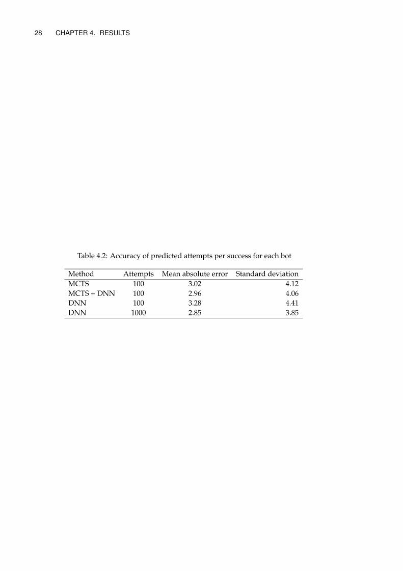
4.3 Difficulty Predictions

Table 4.2 shows the mean absolute errors on 361 levels for each bots. It shows how wellthe model could predict human difficulty from the bots difficulty.

The most surprising result is that even though the DNN is much weaker than MCTSit is about as good or better at predicting human difficulty when it is allowed to make1000 attempts per level instead of 100 as can be seen in Table 4.2. When the DNN onlymakes 100 attempts per level it is the worst predictor. Since the DNN is much faster thanMCTS it can make 1000 attempts in much shorter time than MCTS makes 100 attempts.

28 CHAPTER 4. RESULTS

Table 4.2: Accuracy of predicted attempts per success for each bot

Method Attempts Mean absolute error Standard deviationMCTS 100 3.02 4.12MCTS + DNN 100 2.96 4.06DNN 100 3.28 4.41DNN 1000 2.85 3.85

Chapter 5

Discussion & Conclusions

5.1 Practical Usefulness

The fact that the DNN can make comparable difficulty predictions to MCTS if it is al-lowed to make 1000 attempts instead of 100 attempts is a practically useful result. Itmeans that comparable estimations of human difficulty can be obtained in minutes in-stead of hours. This can change the level designers work flow giving them a much fasterfeedback loop making more tweaks possible before release.

5.2 Method Applicability Outside Candy Crush Saga

The method we used to predict game level difficulty in Candy Crush Saga should be ap-plicable to other games as well. The game need to have a finite action space so it can beinterpreted as a classification problem and since we only looked at the current game stateto select a move, move selection must only depend on the current game state and not theprevious ones. At King we have applied the same method in two other games as wellbut those were very similar to Candy Crush Saga. The method is most useful for gamesthat release new levels frequently.

5.3 Deep Neural Network and Monte Carlo Tree Search Compari-son

The main advantage the DNN approach has is speed, comparable difficulty predictionscan be made in much shorter time. Another benefit with the DNN is that it could betrained on human game play data making it play more like a human could lead to moreaccurate predictions. The main disadvantage with the DNN is that it requires game playdata and retraining. For every new game a game state representation must be createdand data collected. The DNN must be retrained whenever new game elements are addedto the game and new data collected in order to remain accurate. MCTS does not requireany knowledge of the game board and therefore the same algorithm can be applied tonew games without modification.

29

30 CHAPTER 5. DISCUSSION & CONCLUSIONS

5.4 Ethics of Artificial Intelligence

There are two main concerns of Artificial Intelligence (AI). The threat of super intelli-gence and the economic impact of automation.

Super Intelligence

AI can be divided into three categories depending on how powerful it is. Today all AIavailable is in the category artificial narrow intelligence (ANI) which means that it is taskspecific. DeepBlue is better than any human at chess but playing chess is all it can do.The second category is artificial general intelligence (AGI) and includes AI that is aboutas capable as a human, meaning that it is capable of doing general things that humanscan do. The third category is artificial super intelligence (ASI) and consists of AI superiorto human beings. Once AGI is invented, it might be able to recursively improve its soft-ware in order to make it more capable and eventually reach ASI [20]. If ASI turns malig-nant it might send humans to extinction. In this thesis we explore yet another applicationof ANI which in its current state does not pose an existential threat to humanity.

Economic Impact

AI capable of replacing human labor at cheaper prices will cause unemployment, at leasttemporarily while redundant workers find replacement work [21]. Some workers mayfind it hard to transition to new occupations as they may not have or be capable of ac-quiring skills demanded. This thesis might make manual testers of games redundant andunemployed.

Environmental Impact

The method described need computational power and storage on cloud servers but hav-ing a computer program play a level in a few seconds should have a much smaller en-vironmental impact than having a human being playing it in a few minutes so we arguethat successfully replacing manual play testers with an automated solution is good forthe environment.

5.5 Future Work

Improve Architecture

As we were heavily restricted by time we did not investigate the space of possible neuralnetworks very much. There is an almost infinite number of things one could try. If onehas time then training a deeper DNN with more data would likely show better results.We did not overfit with our architecture so training a deeper DNN would be the nextthing to try.

Improve Data

The data we used excluded important information such as the goal of the level. It alsodid not contain the direction of moves. Using better data would likely show better re-sults.

CHAPTER 5. DISCUSSION & CONCLUSIONS 31

Real User Data

We initially intended to use real user data for this thesis. We spent a lot of time collect-ing it for Candy Crush Soda Saga which required adding code to the code base and get-ting it released. It was however aborted as there were problems replaying the games out-side of our control. It would be interesting to continue this experiment and train on ex-pert players and see what that does for performance.

Reinforcement Learning

In this thesis we only attempted to make the neural network learn how someone elseplays, in this case an MCTS bot. The performance metric being minimized is how wellthe neural network can predict how someone else would play. It could be interestingto change the aim to play as good as possible. Using reinforcement learning the DNNweights could be altered after having been trained on a dataset to maximize its perfor-mance. Play a level, see how well it performed, update the weights in order to make itplay better the next time.

Qualitative Exploration of Learning

We only made quantitative measurements of performance. What kind of moves andstrategies does the neural network learn? We have no idea, we only know that it gets acertain validation accuracy and that it gets a certain success rate in a game. Exploringwhat kind of moves it learns and does not learn could perhaps give some interesting in-sights.

5.6 Conclusions

We investigated using a bot based on a DNN playing the game Candy Crush Saga in or-der to predict game level difficulty and compared it to a bot based on MCTS. We trainedthe DNN on data generated by the MCTS bot. The DNN bot is much weaker than theMCTS bot but it could be used to make predictions of human difficulty comparable tothe MCTS bot in much shorter time. The DNN can also be used to make the MCTS boteven stronger by using it during playouts instead of random playouts but the predictionsof human difficulty made from it were not more accurate. The three most important con-clusions are:

• MCTS is much stronger than DNN

• DNN can make MCTS even stronger if used during playouts

• DNN can make comparable predictions of human difficulty in substantially shortertime

Bibliography

[1] David Silver, Aja Huang, Christopher J. Maddison, Arthur Guez, Laurent Sifre,George van den Driessche, Julian Schrittwieser, Ioannis Antonoglou, Veda Pan-neershelvam, Marc Lanctot, Sander Dieleman, Dominik Grewe, John Nham,Nal Kalchbrenner, Ilya Sutskever, Timothy Lillicrap, Madeleine Leach, Ko-ray Kavukcuoglu, Thore Graepel, and Demis Hassabis. Mastering the gameof go with deep neural networks and tree search. Nature, 529:484–503, 2016. URLhttp://www.nature.com/nature/journal/v529/n7587/full/nature16961.html.

[2] Erik Poromaa. Crushing candy crush. Master’s thesis, Royal Institute of Technology,Brinellvägen 8, 2016.

[3] Alex Krizhevsky, Ilya Sutskever, and Geoffrey E Hinton. Imagenet classification withdeep convolutional neural networks. In Advances in neural information processing sys-tems, pages 1097–1105, 2012.

[4] Chris J. Maddison, Aja Huang, Ilya Sutskever, and David Silver. Move evaluationin go using deep convolutional neural networks. CoRR, abs/1412.6564, 2014. URLhttp://arxiv.org/abs/1412.6564.

[5] Barak Oshri and Nishith Khandwala. Predicting moves in chess using convolutionalneural networks.

[6] Volodymyr Mnih, Koray Kavukcuoglu, David Silver, Alex Graves, IoannisAntonoglou, Daan Wierstra, and Martin Riedmiller. Playing atari with deep rein-forcement learning. arXiv preprint arXiv:1312.5602, 2013.

[7] Levente Kocsis and Csaba Szepesvári. Bandit based monte-carlo planning. In Euro-pean conference on machine learning, pages 282–293. Springer, 2006.

[8] Yann LeCun, Yoshua Bengio, and Geoffrey Hinton. Deep learning. Nature, 521(7553):436–444, 2015.

[9] Djork-Arné Clevert, Thomas Unterthiner, and Sepp Hochreiter. Fast and accuratedeep network learning by exponential linear units (elus). CoRR, abs/1511.07289,2015. URL http://arxiv.org/abs/1511.07289.

[10] Pavel Golik, Patrick Doetsch, and Hermann Ney. Cross-entropy vs. squared errortraining: a theoretical and experimental comparison. In Interspeech, pages 1756–1760,2013.

32

BIBLIOGRAPHY 33

[11] Douglas M Kline and Victor L Berardi. Revisiting squared-error and cross-entropyfunctions for training neural network classifiers. Neural Computing & Applications, 14(4):310–318, 2005.

[12] Rob A Dunne and Norm A Campbell. On the pairing of the softmax activation andcross-entropy penalty functions and the derivation of the softmax activation func-tion. In Proc. 8th Aust. Conf. on the Neural Networks, Melbourne, 181, volume 185, 1997.

[13] Michael A. Nielsen. Neural Networks and Deep Learning. Determination Press, 2015.

[14] James Bergstra and Yoshua Bengio. Random search for hyper-parameter optimiza-tion. Journal of Machine Learning Research, 13(Feb):281–305, 2012.

[15] Barret Zoph and Quoc V. Le. Neural architecture search with reinforcement learning.CoRR, abs/1611.01578, 2016. URL http://arxiv.org/abs/1611.01578.

[16] Christian Szegedy, Wei Liu, Yangqing Jia, Pierre Sermanet, Scott Reed, DragomirAnguelov, Dumitru Erhan, Vincent Vanhoucke, and Andrew Rabinovich. Goingdeeper with convolutions. In Proceedings of the IEEE Conference on Computer Visionand Pattern Recognition, pages 1–9, 2015.

[17] Toby Walsh. Candy crush is np-hard. CoRR, abs/1403.1911, 2014. URLhttp://arxiv.org/abs/1403.1911.

[18] Martín Abadi, Paul Barham, Jianmin Chen, Zhifeng Chen, Andy Davis, Jeffrey Dean,Matthieu Devin, Sanjay Ghemawat, Geoffrey Irving, Michael Isard, et al. Tensorflow:A system for large-scale machine learning. In Proceedings of the 12th USENIX Sympo-sium on Operating Systems Design and Implementation (OSDI). Savannah, Georgia, USA,2016.

[19] Soheil Bahrampour, Naveen Ramakrishnan, Lukas Schott, and Mohak Shah.Comparative study of deep learning software frameworks. arXiv preprintarXiv:1511.06435, 2015.

[20] Nick Bostrom. How long before superintelligence? 1998.

[21] Nils J Nilsson. Artificial intelligence, employment, and income. AI magazine, 5(2):5,1984.

www.kth.se

Predicting Game Level Difficulty Using Deep Neural...

Documents

Transcript of Predicting Game Level Difficulty Using Deep Neural...