1

Paper 9820-2016

Predicting Current Market Value of a Housing Unit across the Four Census Regions of the United States Using SAS® Enterprise Miner™

Mostakim Tanjil and Goutam Chakraborty, Oklahoma State University

ABSTRACT

In early 2006, the United States experienced a housing bubble that affected over half of the American states. It was one of the leading causes of the 2007-2008 financial recession. Primarily, the overvaluation of housing units resulted in foreclosures and prolonged unemployment during and after the recession period. The main objective of this study is to predict the current market value of a housing unit with respect to fair market rent, census region, metropolitan statistical area, area median income, household income, poverty income, number of units in the building, number of bedrooms in the unit, utility costs, other costs of the unit, and so on, to determine which factors affect the market value of the housing unit. For the purpose of this study, data was collected from the Housing Affordability Data System of the US Department of Housing and Urban Development. The data set contains 20 variables and 36,675 observations. To select the best possible input variables, several variable selection techniques were used. For example, LARS (least angle regression), LASSO (least absolute shrinkage and selection operator), adaptive LASSO, variable selection, variable clustering, stepwise regression, (PCA) principal component analysis only with numeric variables, and PCA with all variables were all tested. After selecting input variables, numerous modeling techniques were applied to predict the current market value of a housing unit. An in-depth analysis of the findings revealed that the current market value of a housing unit is significantly affected by the fair market rent, insurance and other costs, structure type, household income, and more. Furthermore, a higher household income and median income of an area are associated with a higher market value of a housing unit.

INTRODUCTION

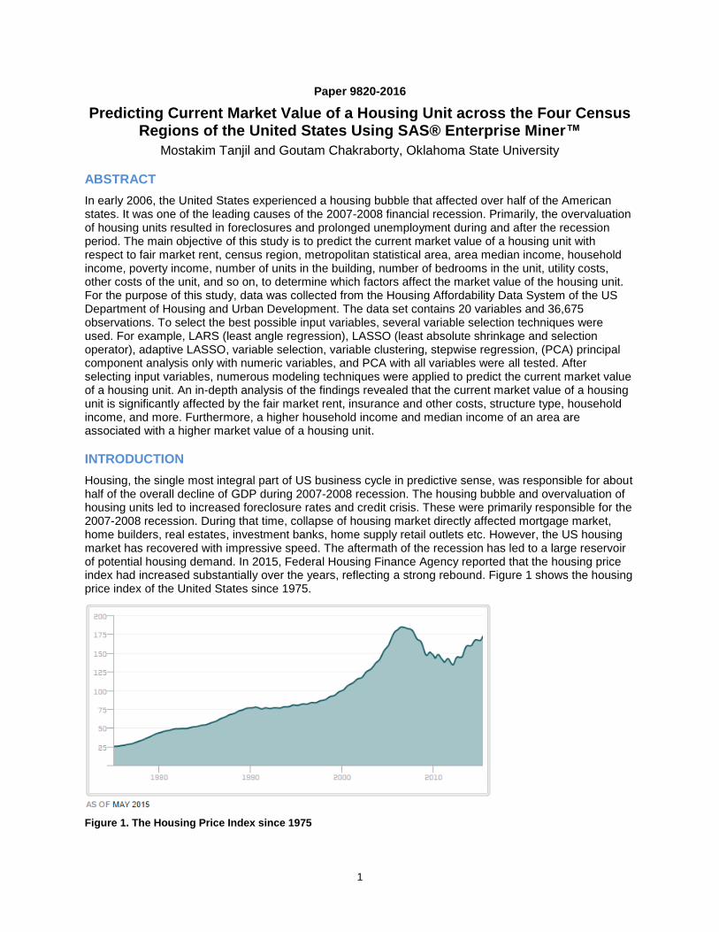
Housing, the single most integral part of US business cycle in predictive sense, was responsible for about half of the overall decline of GDP during 2007-2008 recession. The housing bubble and overvaluation of housing units led to increased foreclosure rates and credit crisis. These were primarily responsible for the 2007-2008 recession. During that time, collapse of housing market directly affected mortgage market, home builders, real estates, investment banks, home supply retail outlets etc. However, the US housing market has recovered with impressive speed. The aftermath of the recession has led to a large reservoir of potential housing demand. In 2015, Federal Housing Finance Agency reported that the housing price index had increased substantially over the years, reflecting a strong rebound. Figure 1 shows the housing price index of the United States since 1975.

Figure 1. The Housing Price Index since 1975

2

Although the housing market has a steady growth for last few years, proper valuation of housing units is mandatory to keep the upward momentum stable and to avoid disastrous subprime defaults. Therefore, the purposes of the study are

To predict current market value of a housing unit across the five metropolitan statistical areas (MSA) in the four census regions of the United States.

To determine factors that affect current market value of a housing unit.

Figure 2. The Four Census Regions of the United States

Figure 2 depicts how the states are grouped by the United States Census Bureau into four regions.

SIGNIFICANCE OF THE STUDY

The main objective of the study is to provide a real life price estimation of a housing unit in all the MSA areas in the four census regions of the United States. The findings of the study will primarily help avoid over valuation of a housing unit both from borrowers’ and lenders’ perspective. Proper application of the outcomes of this research will help lending companies, banks etc. to evaluate a housing unit in relation to geographical location, fair market rent, median income of an area, household income etc. and to fix appropriate mortgage rate. From owners’ standpoint, they will know how much to ask for their houses in relation to the vicinity. The findings of the study will also help people to estimate housing costs as fraction of their income when they consider relocating to different places.

DATA COLLECTION AND PREPARATION

The data was collected from The Housing Affordability Data System of the US Department of Housing and Urban Development. The main data sources are the American Housing Survey (AHS) national sample micro data and AHS metropolitan sample micro data which are conducted every odd year. The data used in this study was collected from the latest AHS survey conducted in 2013. The final dataset has 36,675 observations with 19 predictor variables and one interval target variables. Details are given in the data dictionary in the

Table 1.

3

Variable Level Description

CONTROL ID Each housing unit has a 12-digit unique ID

METRO3 Nominal 1 - 5, 1=Central city of Metropolitan Statistical Areas (MSA), 2 = Inside MSA-urban, 3 = Inside MSA-rural, 4 = Outside MSA-urban, 5 = Outside MSA-rural

REGION Nominal 1 - 4 Census Region, 1 = Northeast, 2 = Midwest, 3 = South, 4 = West

BUILT Nominal Year the unit was built, 29 levels

ZADEQ Nominal 1 - 4, 1 = Adequate, 2 = Moderately inadequate, 3 = Severely inadequate, 4 = Not applicable

STRUCTURE_TYPE Nominal 1 - 6, 1 = Single house, 2 = 2-4 units apartment complex, 3 = 5-19 units apartment complex, 4 = 20-49 units apartment complex, 5 = 50+ units apartment complex, 6 = Mobile home

LMED Interval Area median income in US dollars

FMR Interval Fair market rent in US dollars

L80 Interval Low income limit of the area in US dollars

IPOV Interval Poverty income of the area in US dollars

BDRMS Interval Number of bedrooms in the unit

NUNITS Interval Number of units in the building

ROOMS Interval Total number of rooms in the unit

UTILITY Interval Monthly utility cost of the unit in US dollars

OTHER_COST Interval Monthly insurance, condo, land rent, mobile home fees in US dollars

APLMED Interval Median income adjusted for number of person in the family in US dollars

BURDEN Interval Housing cost as a fraction of income

ZINC2 Interval Household income in US dollars

VALUE Interval Current market value of the unit in US dollars

Table 1. Data Dictionary for the Final Dataset

Four of the variables had missing values which were imputed using decision tree method based on higher similarities and attribute correlations to maximize utilization of observations during model building step. The

Table 2 shows the number of observations and method of imputation of the four variables.

Table 2. Imputation Summary of Missing Values

4

DATA EXPLORATION

Visual data exploration was conducted as the first step of data analysis. Visualization helped to explore implicit patterns and relationships between variables that helped in the model building approach later on.

Figure 3. Mean of Current Market Value of Housing Units Plotted against Central City/Suburban Status (left) and Number of Bedrooms (right) for Four Census Regions

Current mean market values of units are higher for the Northeast and West region of the US compared to the Midwest and South region. For both the Northeast and West region, housing units inside a metropolitan urban area are the most expensive followed by units in metropolitan central city and metropolitan rural area. Although downtowns are the central business districts and considered commercial heart of a city, people tend to pay higher for housing units which are inside metropolitan areas but not within downtown areas. For Midwest and South region, housing prices do not vary substantially depending on the location of housing units. However, regardless of region, prices of housing units increase gradually with the number of bedrooms in a unit. The only exception is efficiency/studio (zero bedroom) housing units in the West region which value more than one, two and three-bedroom housing units (

Figure 3). Furthermore, irrespective to census region and location, three-bedroom housing units are the most common and their accumulated prices are the highest followed by four bedroom units (

Figure 4).

Figure 4. Total Market Value of Housing Units across the Four Census Regions

Figure 5 illustrates that FMR (fair market rent) is slightly higher for the Northeast and West region of The United States, and inside MSA urban areas it is the highest for all census regions. However, plotting of

5

current market values of units against FMR and urban status did not reveal any obvious association and pattern.

Figure 5. FMR in Relation to Census Regions and Current Market Value of a Unit

Monthly utility bills go up with the number of bedrooms in the unit, however, other costs (insurance, condo, land rent and other mobile home fees) are higher for fewer bedroom housing units, especially inside central city and metropolitan urban areas. In addition, visual exploration also illustrates that monthly utility cost is not strongly related to current market value of units, nevertheless, lower other costs appear to be associated with higher current market value of units (

Figure 6).

Figure 6. Monthly Utility Bills and Other Costs in Relation to Current Market Value and Number of Bedrooms

Figure 7 depicts that irrespective to census region, number of units in the building is the highest for central cities. It is reasonable for central cities to have higher number of units in a building as skyscrapers and high-rise buildings are predominantly in the central cities. On the other hand, most of the buildings in urban areas are single-unit residential buildings.

6

Figure 7. Number of Units in a Building across the Five Urban Areas

MODEL BUILDING

At first, the imputed dataset was split into 40% training, 30% validation and 30% test. Making three partitions provided fairly large number of observations to perform honest assessment in terms of validation and test. Six of the variables: IPOV, BURDEN, ZINC2, NUNITS, OTHER_COST, UTILITY and VALUE were transformed to obtain symmetric distribution with respect to lower skewness and kurtosis values.

One of the core assumptions of most parametric multivariate techniques is the absence of multivariate outliers. However, multivariate outliers may not be outliers in univariate distribution, and they are hard to detect when dimension exceeds two. For this study, the basis for multivariate outlier detection was the Mahalanobis distance which was computed by the following formula for each data point Xi.

MD = √(𝑋𝑖 − 𝑇(𝑋)) 𝐶(𝑋)−1(𝑋𝑖 − 𝑇(𝑋))

Where, T(X) is the arithmetic mean of the dataset X and C(X) is the sample covariance matrix. The distance MD shows how far Xi is from center of the cloud, taking into account the shape of the cloud.

Following SAS code is used to detect outliers based on Mahalanobis distance to mean. The code is taken from SAS® support web site.

Title 'Find Mahalanobis distance from each point to the mean';

proc princomp data=&em_import_data std out=out outstat=outstat noprint;

var %EM_INTERVAL;

run;

data mahalanobis_to_mean;

set out;

mahalanobis_distance_to_mean = sqrt(uss(of prin:));

Dist_df= mahalanobis_distance_to_mean/12;

Prob_Chisq = 1-CDF('CHISQUARE',mahalanobis_distance_to_mean,12);

proc sort ;

by Prob_Chisq;

run;

Data temp;

set mahalanobis_to_mean ;

if dist_df ne '.';

options firstobs=1 obs=2000;

7

proc print data=temp uniform noobs;

id control;

run;

Multivariate outlier detection showed that only one observation can be considered outlier with respect to probability of Chi-square and Mahalanobis distance. Hence, the observation was left unchanged.

To reduce the number of levels of the categorical input variable BUILT, it was consolidated using decision tree method. Consolidation of the variable BUILT resulted in reduction of levels to 5 from 29.

To reduce the number of input variables, LARS, LASSO, Adaptive LASSO, Variable Selection, Stepwise regression with both entry and stay significance level 5%, Variable Clustering, PCA only with numeric variables and PCA with all variables were tested. However, different techniques/nodes provided different number of inputs ranging from 4 to 17. Therefore, to select the best inputs, all the variable selection nodes were connected to the modelling nodes and results of the modelling nodes were compared using the model comparison node.

As the primary target of the study is to predict current market value of a housing unit, test average/mean squared error (ASE) is used as the primary selection criterion. ASE is computed using the following formula.

ASE = 1

𝑛∑ (��𝑖 − 𝑌𝑖)

2𝑛𝑖=1

Where �� is the prediction and 𝑌𝑖 is the observed value.

Different modelling techniques: decision tree with different number of branches and depth, neural network with different number of hidden units and different network architecture (multilayer perceptron, ordinary radial, normalized radial and generalized liner model), Polynomial Regression (two factor interaction with polynomial degree 3), PLS (NIPALS, SVD, Eigenvalue and RLGW algorithm), Gradient Boosting (square error and Huber M-regression loss function), Memory Based Reasoning (MBR) with only numeric variables passed through PCA, MBR with both categorical and numeric variables passed through PCA were applied to predict current market value of a housing unit. For accuracy optimization, each model was iterated several times using different features. However, the model comparison node selected the two neural networks (construction architecture – multilayer perceptron) passed through Adaptive LASSO and Stepwise Regression with single hidden layer with three hidden units as the best model based on test ASE. The same 14 input variables are selected by both Adaptive LASSO and Stepwise Regression – ZADEQ, STRUCTURE_TYPE, UTILITY, IPOV, ROOMS, BUILT, REGION (1,2,3), ZINC2, METRO3, OTHER_COST, BURDEN, L80, APLMED, FMR and BDRMS.

Adaptive LASSO is a specialized regression technique that can be used for both model fitting and prediction, and variable selection. Adaptive LASSO can handle both numeric and categorical variables. In this study, it is used for the purpose of variable selection. Adaptive LASSO fits a constrained form of Ordinary Least Squares Regression where weights are applied to the parameter in the LASSO constraint. The constraint is that the sum of absolute values of all regression coefficients must be smaller than a certain value. The adaptive LASSO estimates are defined as

= 𝑎𝑟𝑔 𝑚𝑖𝑛 ||𝑌 − ∑ 𝑥𝑗𝑗𝑝𝑗=1 ||2 + 𝑛 ∑ ��𝑗|

𝑗|

𝑝𝑗=1

Where 𝑛is the non-negative regularization parameter and ��𝑗 is the adaptive weight.

8

Figure 8. Parameter Estimate (Absolute Values) of the Adaptive LASSO

The above figure illustrates the absolute values of parameter estimates of Adaptive LASSO. The variable L80 (low income limit) has the highest estimate of 0.473. Low income limit, structure type, household income, monthly insurance cost, number of rooms, fair market rent, housing cost as a fraction of income and monthly utility costs have positive effect on current market value of a housing unit. On the other hand, poverty income, median income, MSA areas, year the unit was built, census region (1, 2 & 3), adequacy/condition of a housing unit and number of bedrooms have negative effect on current market value.

Table 3 illustrates comparison of the top eight models based on validation and test ASE. Neural network outperformed all the other models.

Model Validation ASE

Test ASE

Neural Network (Stepwise Regression) 0.311388 0.322367

Neural Network (Adaptive LASSO) 0.311388 0.322367

Polynomial Regression 0.348389 0.351355

Partial Least Square (PLS) 0.354991 0.360689

Decision Tree 0.385548 0.394083

MBR (all variables) 0.401272 0.410471

MBR (numeric variables) 0.423757 0.44369

Gradient Boosting 0.423372 0.445096

9

Table 3. Comparison of Top Eight Models

MODEL FINDINGS

The convergence criteria were satisfied and optimization was achieved at 10 iterations for training for the neural network (Figure 9).

Figure 9. Iteration Plot for the Neural Network

Figure 10 Elucidates that The graph of predicted mean against target mean for the selected neural network for test dataset shows that predicted values lie very close to actual values, implying high efficiency of the neural network.

0

0.05

0.1

0.15

0.2

0.25

0.3

0.35

0.4

0.45

Validation ASE Test ASE

Neural Network (Stepwise Regression) Neural Network (Adaptive LASSO)

Polynomial Regression PLS

Decision Tree MBR (all variables)

MBR (numeric variables) Gradient Boosting

10

Figure 10. Mean Predicted Vs Mean Target Values for the Selected Neural Network Model

To explain architecture of the selected neural network, it was passed through a surrogate decision tree. The order of importance of the variables selected by the surrogate decision trees is: FMR (fair market rent), OTHER_COST (monthly insurance cost etc.), STRUCTURE_TYPE (number of units in the building), ZINC2 (household income), ROOMS (total number of rooms in the unit), BUILT (the year unit was built), BURDEN (housing cost as fraction of income), REGION (census regions), APLMED (median income), BEDRMS (number of bedrooms), L80 (low income limit), METRO3 (MSA area), IPOV (poverty income), ZADEQ (adequacy or condition of the unit) and UTILITY (monthly utility cost of the unit). General explanation of some of the identified rules about the current market value of a unit are as follows:

Housing units which has fair market rent more than $1,892.5, and insurance and other costs less than $54, will have market value of around $261,000.

Mobile homes with fair market rent between $1,231.5 and $1,793.5, and insurance and other costs more than $54 will have market value of around $48,400.

Mobile homes with fair market rent between $1,231.5 and $1,892.5, and insurance and other costs between $28 and $54 will have market value of around $61,800.

Single houses and apartment complex in the census region Northeast and West will have similar market values if fair market rent, and insurance and other costs are similar. Similarly, single houses and apartment complex in Midwest and South region will have comparable market values.

Average household income and median income of the area affect market value of housing units. Higher household and median income are associated with higher market value of housing a unit when all other features are controlled.

Number of units in the building does not affect current market value of a housing unit.

Fair market rent, and insurance and other costs are the two most important factors that are used several times to determine market value of a housing unit.

CONCLUSION

In today’s world, all businesses are interconnected. Contraction in one business sector directly affects all other sectors. Therefore, any collapse or downfall of the US housing market in the future will directly affects nation’s mortgage market, home builders, real estate etc. and overall unemployment rate. In order to account for the uncertainty in property valuation, this paper presents an approach to estimate current market value of a housing unit in the four census regions across the United States based on different factors that highly influence market values. To avoid onset of a housing bubble, which led to the economic recessions in the US in both 1930 and 2008, proper valuation of housing units cannot be overlooked.

11

REFERENCES

Leamer, E. 2015. “Housing Really is the Business Cycle: What Survives the Lessons of 2008-09?”. Journal of Money, Credit and Banking, 47(S1): 43-50.

Reuters. 2015. “Strong U.S. Groundbreaking, Building Permits Boost Housing Outlook”. Accessed July 17, 2015. http://www.reuters.com/article/us-usa-eonomy-housing-idUSKCN0PR1CM20150717.

Federal Reserve Bank of St. Louis. 2015. “All-Transactions Housing Price Index for the United States”. Accessed, July 1, 2015. https://research.stlouisfed.org/fred2/series/USSTHPI.

Federal Housing Finance Agency. 2015. “Housing Price Index”. Accessed July 17, 2015. http://www.fhfa.gov/DataTools/Downloads/Pages/House-Price-Index.aspx.

U.S. Department of Housing and Urban Development. 2016. “American Housing Survey: Housing Affordability Data System”. Accessed May 10, 2015. https://www.huduser.gov/portal/datasets/hads/hads.html.

Rahman, M.G. and Islam, M. Z. 2013. “Missing Value Imputation Using Decision Trees and Decision Forests by Splitting and Merging Records: Two Novel Techniques”. Knowledge Based System. 53: 51-65.

Rousseeuw, P. J. and Van Zomeren, B. C. 1990. “Unmasking Multivariate Outliers and Leverage Points”. Journal of the American Statistical Association, 85(411): 633-639.

SAS. 2008. “Sample 30662: Mahalanobis Distance: From Each Observation to the Mean, from Each Observation to a Specific Observation, between all Possible Pairs”. Accessed July 15, 2015. http://support.sas.com/kb/30/662.html.

Freund, R. J. and Wilson, W. J. 2003. Statistical Methods. 2nd ed. San Diego, CA: Academic Press

Zou, H. 2006. “The Adaptive LASSO and its Oracle Properties”. Journal of the American Statistical Association, 101(476): 1418-1429.

12

CONTACT INFORMATION

Your comments and questions are valued and encouraged. Contact the authors at:

Mostakim Tanjil Oklahoma State University Stillwater, OK, 74078 Email: imran.tanjil@okstate.edu Work Phone: 313-603-1678

Mostakim Tanjil is a master’s student in Design, Housing and Merchandising at College of Human Sciences of Oklahoma State University (OSU). He is also pursuing Graduate Certificate in Business

Datamining, and SAS and OSU Predictive Analytics Certification from Spears School of Business, OSU. He works as an analyst (graduate assistant) at Center of Health Systems Innovation of OSU. He has a Bachelor of Science in Textile Engineering. Before joining the graduate program, he worked five and a half years for two textile manufacturing industries in Bangladesh as a Senior Engineer. He holds SAS

Certified Base Programmer for SAS9, SAS Certified Statistical Business Analyst Using SAS 9:

Regression and Modeling, SAS Certified Predictive Modeler Using SAS Enterprise Miner 13 credentials. He presented a paper in AATCC International Conference 2015 and a poster in Analytics Conference 2015.

Goutam Chakraborty, Ph. D. Oklahoma State University Stillwater, OK, 74078 Email: goutam.chakraborty@okstate.edu

Dr. Goutam Chakraborty is a Ralph A. and Peggy A. Brenneman professor of marketing and director of Master of Science in Business Analytics at Oklahoma State University. He is the founder of SAS and OSU Datamining Certificate and SAS and OSU Marketing Analytics Certificate. He has published in many journals including Journal of Interactive Marketing, Journal of Advertising Research, Journal of Advertising, Journal of Business Research etc. He has over 25 years of experience in using SAS® for data analysis. He is also a business knowledge instructor for SAS®.