NATIONALEKONOMISKA INSTITUTIONEN Uppsala Universitet Examensarbete D Författare: Gabriel Söderberg Handledare: Nils Gottfries Termin och år: Vårterminen 2005

Predicting Currency Crises – Possible or Impossible?

Abstract

This paper is an assessment of the possibility to predict currency crises. Different methods are

explored. A discrete-choice model is estimated with an underlying intuition that is far more

simple than traditional estimations of this kind. The results suggest that currency crises are

complex phenomenas that cannot be predicted by just using a few variables. I then turn to a

descriptive analysis, that first focuses on macroeconomic fundamentals and then on domestic

troubles in the banking sectors of crisis-struck countries. Finally some possible contributing

factors lying outside the control of crisis countries are discussed. The final conclusion is that

the exact timing of a currency crisis cannot be predicted, but that vulnerability – that is a high

probablity that a crisis can occur – can be detected. Further research on what finally triggers a

crisis in a vulnerable situation is therefore needed.

Acknowledgements

I would like to thank the following people (in alphabetical order): Nils Gottfries for generally

being a good supervisor; Per Johansson for statistical support; Peter Nilsson for useful

suggestions and statistical support; Erik Post for literature tips

2

Contents

1. Introduction...........................................................................................................................4

2. Theoretical models................................................................................................................5

2.1 First generation...................................................................................................................5

2.2 Second generation...............................................................................................................6

2.3 Third generation..................................................................................................................6

3. Discrete-choice regression....................................................................................................7

3.1 Methodology.......................................................................................................................7

3.2 Empirical specifications......................................................................................................8

3.3 Data&sources......................................................................................................................9

3.4 Results...............................................................................................................................11

4. Descriptive analysis.............................................................................................................13

4.1 Macroeconomic fundamentals..........................................................................................14

4.2 The banking sector............................................................................................................22

4.3 External factors.................................................................................................................31

5. Conclusion and summary...................................................................................................35

References................................................................................................................................37

Appendix..................................................................................................................................40

3

1. Introduction The last decades have seen the frustration of many countries as they battle against pressure on

their fixed exchange rates. Often this pressure is overpowering, forcing the country to devalue

or let the currency float. The costs involved in these crises can potentially be enormous.

Indonesia for instance lost 13.5 percent of its GDP the year following the crisis 19971, and the

portion of the population qualified as poor increased from 12 to 22 percent.2 With the 1998

population of Indonesia at 213 millions, this means that approximately 21.3 million people

were thrown into poverty. Learning how and why such crises occur, is thus of extreme

importance. And much more important still: if it is possible to predict that given the current

situation a crisis will occur, it might theoretically be possible to prevent it. This paper is an

attempt to evaluate this possibility to predict a currency crisis.

Since the late 1970’s economists have used different approaches for this end.

Each “wave” of crises spawned its very own generation of theoretical models.3 Models in

each generation all share similar assumptions based on the types of crises they were

constructed to explain.Thus the “first generation” models are based on the Latin American

experience of the late seventies and early eighties, the second on the European and Mexican

crises of 1992 and 1995, and the third generation more or less on the Asian crisis of 1997.

More recently a fourth generation is also being introduced. This constant creation of new

models is a reflection of the complex and versatile structure of currency crises. One

explanation is simply not enough, and each of the models that have been suggested has its

own flaws.

In part as a response to the empirical troubles of the theoretical models, the so

called “leading indicator” approach has been suggested.4 In this the researcher tries different

means to measure a country’s vulnerability to a crisis, or to predict one, using a set of

indicators that reflects all possible causes of the theoretical models mentioned above. This

approach thus tries to “side step” the theoretical literature, instead using some sort of

underlying intuition in choosing its indicators. There are three main methods for doing this.

The signaling method (i) tries to find a crisis “alarm clock” that goes off when one or more

variables exceed a certain threshold. The discrete-choice method (ii) instead uses binary

1 Perkins et al (2001) 2 There might be a problem of causality here: does the crisis cause the downfall or does the downfall cause the crisis? 3 Breuer(2004) 4 Chui(2002)

4

regression models in order to estimate the probability that a crisis occurs given a set of

indicators. And finally the third method is a more descriptive analysis of different case studies

(iii), sometimes by creating a statistical model but often by non-quantitative evaluations of a

country’s situation.

In this paper – as means to assess the possibility to predict currency crises – the

discrete-choice and the descriptive methods will be used. First two separate logit models are

estimated – one for developing and one for industrialized countries. I then turn to a

descriptive analysis first of macroeconomic fundamentals and then on the general status of the

banking sector in different countries. This yields the conclusion that the exact timing of a

currency crisis is probably impossible to predict, but that vulnerability to crisis should be

possible to detect. Therefore predicting crisis seems to be equivalent to finding situations

were crises can suddenly erupt, although the triggering causes are not fully understood at this

time.

The rest of this paper is organized as follows. In section 2, I briefly describe the

theoretical models. Section 3 describes and presents the results of a discrete-choice

regression. Section 4 is a descriptive analysis of a number of cases, analyzing whether the

crisis in Asia 1997 could have been predicted by finding similarities with the then rather

recently crisis-struck countries of Finland, Mexico, and Sweden. Finally, section 5 includes

summary and a conclusion.

2.Theoretical models There are mainly three different types of models, often called the first, second, and third

generations. Each of these generations contains a number of different models that share

several similarities, and are generally based on a certain wave of crises that hit a region in a

particular time period. I here very briefly describe these three generations.5

2.1 First generation

The experiences of the Latin American countries in the 1970’s and 1980’s served as

foundation for the earliest models. These countries typically had large budget deficits which

the government financed by borrowing from the central bank. This together with large current

account deficits followed by large capital outflows led to problems that ended with a drop in

the fixed rate. The first generation models thus try to explain how and why this happens. For

5 The following is based on Breuer(2004) and Saxena(2004)

5

example the Krugman model (1979), assumes that the government is financing its debt by

borrowing from the central bank while the central bank must use its foreign reserve to keep

the exchange rate at a fixed level. This situation is unsustainable: sooner or later the central

bank must run out of foreign currency. Speculators – assumed to have perfect foresight –

realize this and will stage an attack in order to profit from the discrete jump in the exchange

rate as it is depreciated. Competition among these speculators, however, pushes the timing of

the attack backwards, so that it will occur before the central bank has run out of reserves. This

means that there is no jump in the exchange rate although it starts to depreciate continuously.

2.2 Second generation

The European crises in 1992 and 1993 were different from the ones in Latin America. There

were no severe macroeconomic problems, and no inconsistencies between the keeping of a

fixed exchange rate and financing of the budget deficit. Instead these countries were hit by

massive speculative attacks, leading them to devaluate or float their currencies long before

their central banks were insolvent. Most of these countries had the means to continue

protecting their exchange rates but chose not to. The prevalent model – Obstfeld (1994) - thus

focuses on self-fulfilling crises, that is crises created by people’s expectations, and the fact

that the government chooses whether to defend the exchange rate or not out of the perspective

of optimizing utility. Currency crisis can therefore theoretically occur in a relatively good

economic environment, simply because pessimistic investors withdraw their money and the

government finds that protecting the exchange rate is more costly than letting it go.

2.3 Third generation

The Asian crises in 1997, and the fact that none of the earlier models were sufficient to

explain it, created interest in the workings of the banking sector. Thus the “twin crisis”

concept was introduced, underlining the connection between banking and currency crises.

Here there is a huge number of different models and no one has become prevalent in the way

that the Krugman and Obstfeld models have. Often these models cointain elements from the

earlier generations, mainly the concept self-fulfilling crisis.6 Most of them focus on over-

lending to risky projects which makes the country vulnerable to external shocks. In this way

the occurrence of a banking crisis – a large amount of non-performing loans that hurt the

banking sector – can trigger a currency crisis for example through capital flight as investors

6 Chui(2002)

6

realize the weakness of the country. Also a situation with highly debt-levered firms raises the

cost for protecting the fixed exchange rate through interest rate increases and thus increasing

the government incentive to devalue if faced with pressure. This might lead to a speculative

attack.

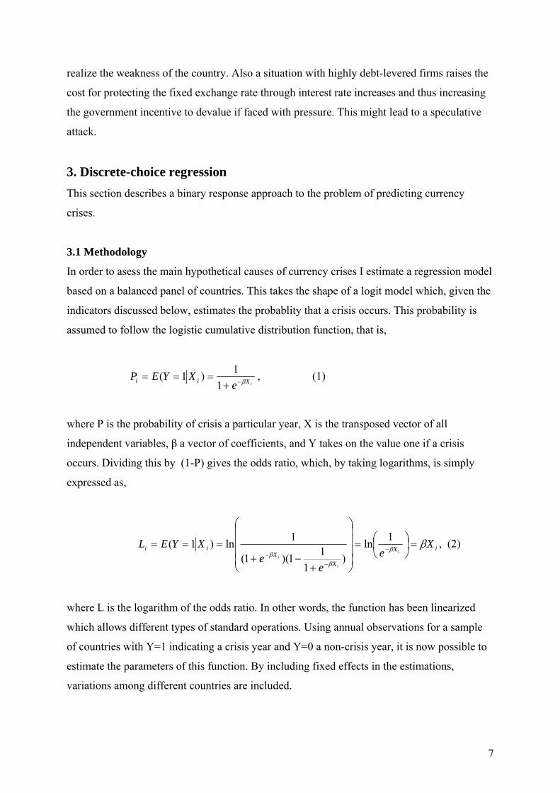
3. Discrete-choice regression This section describes a binary response approach to the problem of predicting currency

crises.

3.1 Methodology

In order to asess the main hypothetical causes of currency crises I estimate a regression model

based on a balanced panel of countries. This takes the shape of a logit model which, given the

indicators discussed below, estimates the probablity that a crisis occurs. This probability is

assumed to follow the logistic cumulative distribution function, that is,

iXii e

XYEP β−+===

11)1( , (1)

where P is the probability of crisis a particular year, X is the transposed vector of all

independent variables, β a vector of coefficients, and Y takes on the value one if a crisis

occurs. Dividing this by (1-P) gives the odds ratio, which, by taking logarithms, is simply

expressed as,

iX

XX

ii Xe

ee

XYELi

i

i

ββ

ββ

=⎟⎠⎞

⎜⎝⎛=

⎟⎟⎟⎟

⎠

⎞

⎜⎜⎜⎜

⎝

⎛

+−+

=== −

−−

1ln)

111)(1(

1ln)1( , (2)

where L is the logarithm of the odds ratio. In other words, the function has been linearized

which allows different types of standard operations. Using annual observations for a sample

of countries with Y=1 indicating a crisis year and Y=0 a non-crisis year, it is now possible to

estimate the parameters of this function. By including fixed effects in the estimations,

variations among different countries are included.

7

3.2 Empirical specifications

Earlier theories and observations leads me to focus on four factors: current

account deficits, government budget deficits, poor growth of domestic output, and worsening

international competitiveness. Current account and budget deficits are scaled by expressing

them as percentage of GDP. The other two hypothesized causes are trickier to deal with. In

order to model the impact of possible problems within the domestic economy, I created an

index of actual output compared to its trend. This “output gap” is defined as the difference

between the logarithm of real GDP and its Hodrick-Prescott trend. Also, international

competitiveness is measured by the percent increase in real effective exchange rate over a

period of three years7. The included indicators and their theoretical motivations are thus as

follows. Current account: A current account deficit means that a country is having a foreign

debt that might lead to strain on the currency reserves if creditors choose to withdraw their

investments. Budget balance: A budget deficit might mean that the government is tempted to

use inflation as a source of revenue, also putting pressure on the foreign reserves. Output gap:

Low domestic output means a signal of economic weakness, suggesting to investors that the

country is not worthy of the funds invested in it. Real effective exchange rate appreciation:

Worsening competitiveness might suggest that a devaluation is needed in order to put the

export industry back on track.

All indicators were lagged one period in the regression. Thus the function to

be estimated is:

ttt

ttt

tt

REERGAP

GDPBBGDPCAP

PL

εββ

ββα

+∆++

++=−

=

−−

−−

1413

12111 //1

ˆ (3)

where (CA/GDP) denotes current account as percentage of GDP, (BB/GDP) government

budget balance as percentage of GDP, GAP the output gap, and ∆REER the percent three

year change in real effective exchange rate8.

Table 1 summarizes the expected signs of the estimated coefficients. The current

account as percentage of GDP should be negative, that is a deficit increases the chance of a

crisis. For the same reason budget balance as percentage of GDP and output gap should have

7 The real effective exchange rate is calculated by giving other countries a weight according to their importance as trade partners. 8 Estimating with fixed effects means giving each country but one a dummy variable that influences the intercept. The full function to be estimated is thus:

tttnnt REERGAPGDPBBGDPCADDL εββββααα +∆+++++++= −−− 1413211121 //...ˆ

8

negative coefficients. The coefficient for the real effective exchange, though, should be

positive since a high value on this suggests hard times for the export industry.

Table 1. Expected signs of estimated coefficients

Indicator Expected sign

CA/GDP -

BB/GDP -

GAP -

∆REER +

3.3 Data&sources

My approach to the discrete-choice method of predicting currency crises, and therefore the

underlying causes, is in several ways different from similar estimations in the past. First of all,

it is very parsimonious: I include only four explaining variables, whereas Frankel and Rose

(1996) include seventeen, Kumar, Moorthy, and Perraudin (1998) thirty-two, and

Komulainen (2004) twenty-three. Secondly, my model – in relation to its modest size – is

based on the simplest possible intuition. The underlying intuitions in other empirical models

are far more complex, including such variables as short term debt, central bank currency

reserves, and foreign direct investment. One can be sceptical about these approaches, since

including so many different variables entails great risk of multicollinearity. Also, variables

with weak intuitive justification are sometimes included. Thus, if the estimated parsimonous

model is inadequate to predict crises, the use of more complex models is to some extent

justified.

Thirdly, there is the difficult question of defining a crisis. This generally

includes some arbitrariness. Frankel and Rose for instance use a more than twenty-five

percent depreciation of the nominal exchange rate together with an increase of ten percent in

the rate of depreciation. I instead use a depreciation of more than eight percent of the nominal

effective exchange rate for a country with fixed exchange rate. This value was chosen after

reviewing “known” crises and their percent depreciations. Still the reader should bear in mind

that both my approach and the others are bound to miss some crises, since the floating of a

previously fixed exchange rate does not necessarily mean that it depreciates to a great extent.

The French experience during 1992 is an example of this situation: the country was forced to

9

abandon its peg and let the Franc float, but its nominal value only depreciated a few

percentage points. This crisis can not be detected using a measure of depreciation. Other

definitions have similar types of problems.

I estimate two different panel regression models: one for industrialized

countries, and one for developing countries. The reason for this is that one could assume that

these two groups would behave differently when faced with crisis pressure and thus be

inequally sensitive. An industrialized country might for example avoid crisis in spite of a huge

current account or budget deficit while a development country might not. Investors might for

example have lower confidence in the ability of developing countries to deal with their

problems and thus withdraw their money before assumed chaos erupts. Thus it seems a good

idea to keep these two groups separate, although still including newly industrialized countries,

such as South Korea, in the development country category.

In both groups I only include periods with fixed exchange rate regimes. The

definitions of these are taken from Reinhart and Rogoff (2002). I characterize “fixed

exchange rate regime” as everything apart from managed floating and freely floating, that is I

include moving pegs, bands around other currencies, and so on. None of the other studies

seem to have done this, trading a greater number of observations against the unreliability of

including observations where a currency crisis in the usual sense cannot occur – simply

because there is no peg to come under pressure.

The quality of the data can be questioned. For many countries – especially

developing countries – there are large gaps in the time series. Furthermore there are a few

extremely peculiar observations that seem safer to remove than to include in an estimation.

Concerning the frequency of observations used, several researchers – among

them Kumar et al and Komulainen – suggest that monthly data better capture the volatile

nature of financial crises. Most of the data are however only available in annual or quarterly

frequency. The observations used in models with monthly frequence are interpolated. While

this is “allowed” I still feel – as do Frankel and Rose – that the benefits of manipulating the

data in this way do not outweigh the potential drawbacks of it. In the words of Gujarati9: “All

such data ‘massaging’ techniques might impose upon the data a systematic pattern that might

not exist in the original data.”

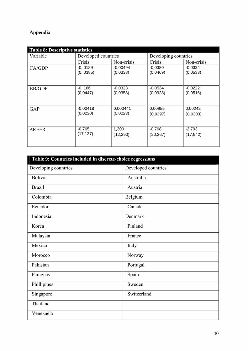
The complete data set used consisted of 15 developing countries, and 13

developed countries, containing time series of the chosen indicators stretching from 1970 to

9 Gujarati(2003)

10

2000. Most of it was taken from IFS Financial Statistics, while some of the development

countries’ real effective exchange rates were taken from J.P Morgan10. Descriptive statistics

and a full list of countries included are found in the appendix.

3.4 Results

The results are somewhat disappointing. In the developing country estimation, only the

intercept and deficit as percentage of GDP are statistically significant, while only the intercept

is significant for industrialized countries. However, the null hypothesis that all variables

collectively have no impact on the probablity of crisis occuring in developing countries is

rejected at 10% level of significance. The same does not hold for industrializes countries

though. In both cases, furthermore, the measure of goodness of fit – McFadden R² - is very

low. The result is summarized in table 2 and 3.

Table 2: Results for Developing Countries

Variable Coefficient (s.e) P-value11 Estimated sign (and

expected)

C -1.205 (0.244) 0.000***

CA/GDP 3.155(4.545) 0.488 +

(-)

BB/GDP -8.567(4.003) 0.0324** -

(-)

GAP 3.714 (7.130) 0.603 +

(-)

∆REER 0.015336 (0.0110) 0.161 +

(+)

P-value (LR-stat) 0.0984* McFadden R² 0.0496

Observations

included: 137

10 The exact definitions in IFS are: CA/GDP=line 78ald/line 99b, BB/GDP=line 80g/line 99b, GDP in fixed prices=lines 99b.p or 99b.r, REER= line rec 11 *** indicates 1% significance, ** 5%, and * 10%

11

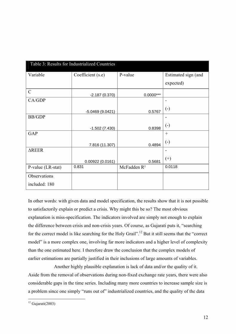
Table 3: Results for Industrialized Countries

Variable Coefficient (s.e) P-value Estimated sign (and

expected)

C -2.187 (0.370) 0.0000***

CA/GDP

-5.0469 (9.0421) 0.5767

-

(-)

BB/GDP

-1.502 (7.430) 0.8398

-

(-)

GAP

7.816 (11.307) 0.4894

+

(-)

∆REER

0.00922 (0.0161) 0.5681

-

(+)

P-value (LR-stat) 0.831 McFadden R² 0.0118

Observations

included: 180

In other words: with given data and model specification, the results show that it is not possible

to satisfactorily explain or predict a crisis. Why might this be so? The most obvious

explanation is miss-specification. The indicators involved are simply not enough to explain

the difference between crisis and non-crisis years. Of course, as Gujarati puts it, “searching

for the correct model is like searching for the Holy Grail”.12 But it still seems that the “correct

model” is a more complex one, involving far more indicators and a higher level of complexity

than the one estimated here. I therefore draw the conclusion that the complex models of

earlier estimations are partially justified in their inclusions of large amounts of variables.

Another highly plausible explanation is lack of data and/or the quality of it.

Aside from the removal of observations during non-fixed exchange rate years, there were also

considerable gaps in the time series. Including many more countries to increase sample size is

a problem since one simply “runs out of” industrialized countries, and the quality of the data 12 Gujarati(2003)

12

detoriates when dealing with smaller and smaller developing countries. Another possible

solution is to estimate the model on a data set consisting of both developed and developing

countries. I did this – including 317 observations – but the results were rather similar to the

ones above.

Since few or none of the indicators were statistically significant analyzing their

estimated coefficent might be a worthless exercise. Still it might be interesting to see if their

signs and sizes are consistent with intution. The only significant indicator – the budget

balance of developing countries – is negative as expected, as is its industrialized counterpart.

The current account however only has the expected sign in the case of industrialized

countries, while outputgap in both cases are positive instead of negative as expected. Finally

the percent increase in real effective exchange rate has expected sign in both estimations.

4. Descriptive analysis The results of the discrete-choice models highlight an important lesson: the phenomenon of

currency crisis is a very complex one. In this section the possibility of prediction is analyzed

in a more qualitiative way.

In this part of the study I will investigate if the crisis in Asia 1997 could have

been predicted. This crisis is interesting mainly for two reasons. First, it was a complete

anomaly in the framework of existing theoretical models13, and thus impossible to predict

applying these. Second, it set off a series of currency crises that followed in its wake – Russia

1998, Argentina and Brazil in 1999. The method used is to compare Asian characteristics the

years preceeding the crisis with those of other countries earlier hit by crises. To this end I

have chosen three reference points: Finland 1992, Mexico 1994, and Sweden 1992. The

reason for choosing these countries is deliberate, since a superficial glance at the crises in

these countries suggests some similarites that should be explored. Given what we knew from

these countries, could the crisis in Asia have been predicted? If this is the case, there have to

important similarities between what happened in Asia 1997 and what happened in Europe

1992 and/or Mexico 1994. Finding such similarities is thus the main aim of my study.

First I evaluate the macroeconomic fundamentals that were extant the years

before the crisis. Then I analyze the suggestions prevalent in third generation models that the

crisis was linked to problems in the banking sector. After that I consider various events lying

outside the control of the crisis countries, such as random events and policy changes in other

13 Saxena(2004)

13

countries. Throughout, the Asian countries will be represented by Thailand. This is for two

reasons. First, the crisis began in Thailand which might mean that all the rest of the countries

were affected in a process of contamination. Second, before the crisis the Thai policies on

attracting foreign capital were widely copied in Asian countries14. Each following sector will

first describe the Thai characteristic, and then more briefly those of the other countries.

4.1 Macroeconomic fundamentals

The East Asian crisis is famous for occurring in a region with stable macroeconomic

indicators. In December 1996 an IMF report titled “Thailand: The Road to Sustained Growth”

apart from a considerable current account deficit found no cause to worry about the country’s

future.15 This was 3 months before speculators attacked the Thai currency in February 199716

- the first of a series of attacks that would finally force the country off its peg. Facts like these

have made some researchers doubt “the usefulness of...macroeconomic variables as warning

signals of vulnerability”.17 I will here investigate this suggestion.

In some cases countries’ paths towards currency crisis from the late 70’s and

onwards had been clearly visible in macroeconomic indicators.18 First the Latin American

experiences, with huge budget deficits financed by high growth rate of money and massive

current account deficits. Then the European crises of the early 90’s typically with

“manageable” budget and current account deficits, but with increasing problems with

unemployment and competitiveness due to falling demand and real exchange rate

appreciations. Finally the Mexican crisis only two years before the Asian, which was

preceded by years of budget surplus, but high inflation, real exchange rate appreciation,

falling growth rate, negative trade balance, and large current account deficits.19

The fundamentals chosen here are: budget balance, current account, growth rate

of GDP, and real effective exchange rate.

Budget balance

First of all Thailand had no problems with government budget deficits. On the contrary, the

Thai government followed an unusually strict spending policy20, perhaps trying to avoid the

14 Allen(1999) 15 Dornbusch(1997) 16 Lauridsen(1998) 17 Lim et al(2004) 18 Saxena(2004) 19 Dornbusch et al(1995) 20 Dornbusch(1997)

14

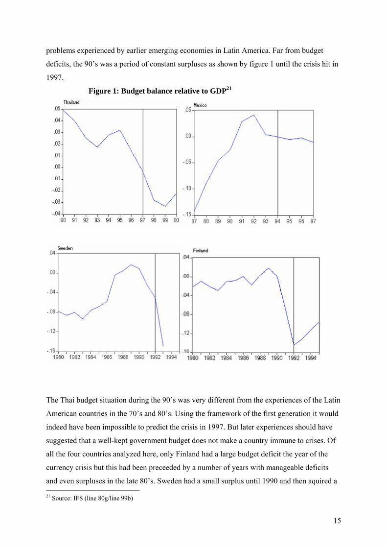
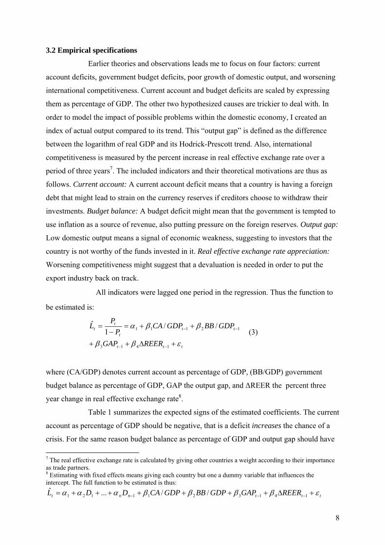
problems experienced by earlier emerging economies in Latin America. Far from budget

deficits, the 90’s was a period of constant surpluses as shown by figure 1 until the crisis hit in

1997.

Figure 1: Budget balance relative to GDP21

The Thai budget situation during the 90’s was very different from the experiences of the Latin

American countries in the 70’s and 80’s. Using the framework of the first generation it would

indeed have been impossible to predict the crisis in 1997. But later experiences should have

suggested that a well-kept government budget does not make a country immune to crises. Of

all the four countries analyzed here, only Finland had a large budget deficit the year of the

currency crisis but this had been preceeded by a number of years with manageable deficits

and even surpluses in the late 80’s. Sweden had a small surplus until 1990 and then aquired a 21 Source: IFS (line 80g/line 99b)

15

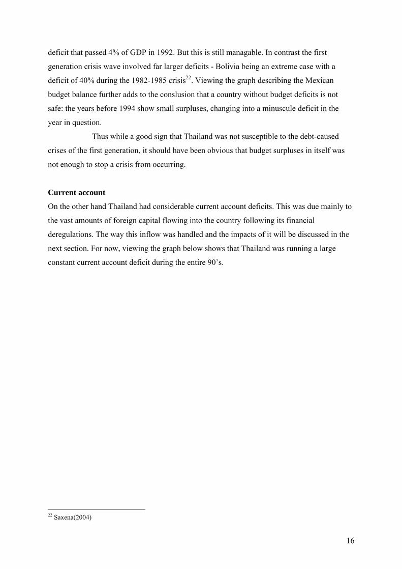
deficit that passed 4% of GDP in 1992. But this is still managable. In contrast the first

generation crisis wave involved far larger deficits - Bolivia being an extreme case with a

deficit of 40% during the 1982-1985 crisis22. Viewing the graph describing the Mexican

budget balance further adds to the conslusion that a country without budget deficits is not

safe: the years before 1994 show small surpluses, changing into a minuscule deficit in the

year in question.

Thus while a good sign that Thailand was not susceptible to the debt-caused

crises of the first generation, it should have been obvious that budget surpluses in itself was

not enough to stop a crisis from occurring.

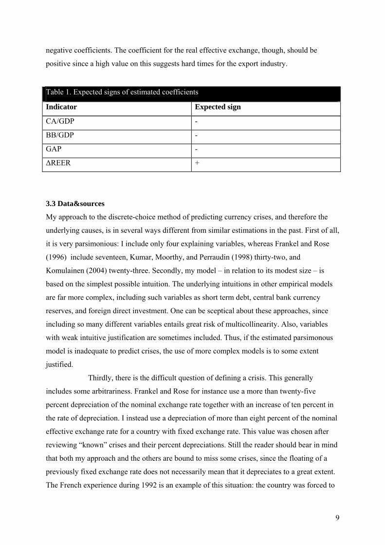
Current account

On the other hand Thailand had considerable current account deficits. This was due mainly to

the vast amounts of foreign capital flowing into the country following its financial

deregulations. The way this inflow was handled and the impacts of it will be discussed in the

next section. For now, viewing the graph below shows that Thailand was running a large

constant current account deficit during the entire 90’s.

22 Saxena(2004)

16

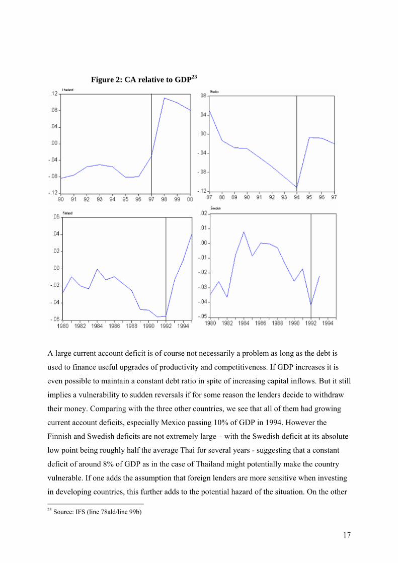
Figure 2: CA relative to GDP23

A large current account deficit is of course not necessarily a problem as long as the debt is

used to finance useful upgrades of productivity and competitiveness. If GDP increases it is

even possible to maintain a constant debt ratio in spite of increasing capital inflows. But it still

implies a vulnerability to sudden reversals if for some reason the lenders decide to withdraw

their money. Comparing with the three other countries, we see that all of them had growing

current account deficits, especially Mexico passing 10% of GDP in 1994. However the

Finnish and Swedish deficits are not extremely large – with the Swedish deficit at its absolute

low point being roughly half the average Thai for several years - suggesting that a constant

deficit of around 8% of GDP as in the case of Thailand might potentially make the country

vulnerable. If one adds the assumption that foreign lenders are more sensitive when investing

in developing countries, this further adds to the potential hazard of the situation. On the other 23 Source: IFS (line 78ald/line 99b)

17

hand Thailand had been running this deficit for years. A large deficit does not necessarily

have to lead to crisis.

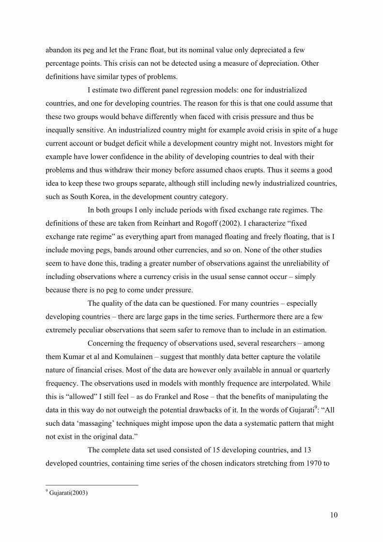
Growth rate of GDP

Both from theory and observation we know that a situation with huge current account deficits

can become a problem if the lenders lose confidence in the country’s ability to repay its debts

in the future or maintain high returns. The indebted country will therefore need to show strong

growth and competitiveness statistics to prove that it is indeed worthy of the capital invested

in it. Also speculators considering launching an attack might draw the conclusion that the

country cannot allow itself to raise interest rates in order to protect the fixed exchange rate.

Looking at the growth rate of GDP for Thailand, one can see that the rate was increasing

slightly for several years and then dropped rather drastically the year before the crisis, from

9.2% to 5.9%.

18

Figure 3: Growth rate of GDP24

The Thai downfall in growth rate might suggest that 1996 was the year in which investors lost

confidence in the country’s ability to handle its debt. But although it fell, a growth rate of

5,9% is a rather healthy one. Finland and Sweden in contrast had much more severe problems.

We see in the graphs that the sharp downfall of growth rate that appeared after the crisis in

Thailand and Mexico appeared before in Finland and Sweden. But although Finland had a

devaluation in 1991 the speculative attacks did not occur until 1992. In Mexico the situation

was slightly different as seen from its graph. Here there was a slow growth rate for many

years and the inflow of capital does not seem to have been able to speed up development.

Thus the slow growth pace of Mexican economic activity was probably one of the reasons for

the problems in 1994.

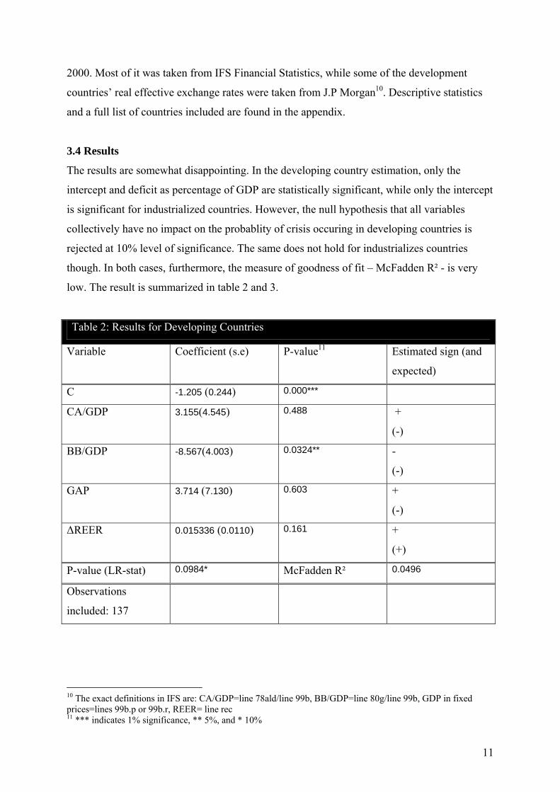
Real effective exchange rate

24 Source IFS (Lines 99 b.p and 99 b.r)

19

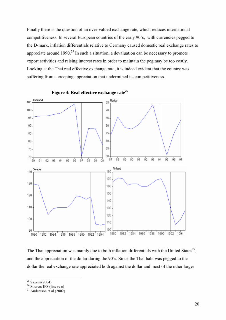
Finally there is the question of an over-valued exchange rate, which reduces international

competitiveness. In several European countries of the early 90’s, with currencies pegged to

the D-mark, inflation differentials relative to Germany caused domestic real exchange rates to

appreciate around 1990.25 In such a situation, a devaluation can be necessary to promote

export activities and raising interest rates in order to maintain the peg may be too costly.

Looking at the Thai real effective exchange rate, it is indeed evident that the country was

suffering from a creeping appreciation that undermined its competitiveness.

Figure 4: Real effective exchange rate26

The Thai appreciation was mainly due to both inflation differentials with the United States27,

and the appreciation of the dollar during the 90’s. Since the Thai baht was pegged to the

dollar the real exchange rate appreciated both against the dollar and most of the other larger

25 Saxena(2004) 26 Source: IFS (line re c) 27 Andersson et al (2002)

20

currencies. This led to harder times for the export industry, as its main advantage of low

wages was undermined, probably contributing to the drop in growth rate we saw in the

previous graph. Finland and Sweden had appreciations in the late 80’s, but it would be wrong

to ascribe all of the following downfall in growth rate to worsening competitiveness, since

there were also problems with falling demand in importing countries – due in large part to the

fall of the Soviet Union, a major trade partner. Visible here is also the Finnish devaluation in

1991. In the case of Mexico, the appreciation was far more severe. The real effective

exchange rate had appreciated rapidly the years before the crisis. This was not enough to send

the growth rate down to negative numbers, but the slow growth rate might well to a great deal

be explained by this, as the stimulation of a profitable export was undermined

Summary and comparison

Comparing Thailand, Finland, Mexico, and Sweden shows several similarities: sound budget

balance (with the exclusion of Finland), current account deficits, some sort of trouble with

growth rate, and real effective exchange rate appreciations. I therefore do not agree that

analyzing the Thai fundamentals “leads one to question the usefulness of...macroeconomic

variables as warning signals of vulnerability”.28 On the contrary, if one defines “vulnerability”

as a setup of macroeconomic variables similar to the setup of a country that afterwards was hit

by a crisis, then I would say that Thailand was indeed becoming vulnerable. Table 5

summarizes some of the similarities.

Table 4: Similarities of compared countries Country Large or

growing budget deficit

Large or growing current account deficit

Low or falling growth rate

Loss of competitiveness

Thailand No Yes Yes Yes Mexico No Yes Yes Yes Sweden No Yes Yes Yes Finland Yes Yes Yes Yes

However, there is a big difference and that is the early response of speculators and investors

following visible troubles. Finland and Sweden had had severe problems since 1990, and

Mexico had had slow growth for several years, while the troubles in Thailand only started to

manifest themselves one year before the crisis. I must therefore conclude that even though

fundamentals suggest that Thailand was heading for a crisis, they are not enough to explain

28 Lim et al(2004)

21

why it finally occurred when it did. From analyzing just fundamentals in 1996, one would

have thought that Thailand had at least two or three years before crisis, while speaking about

“sustained growth” would have been wishful thinking.

4.2 The Banking Sector

Following the Asian crisis was a considerable number of analyses to discern why it had

occurred in spite of manageable macroeconomics.29 Amid many suggested explanations, the

main discussion soon focused on links between banking and currency crises. The banking

sector in the Asian countries was having severe problems, manifested in large amounts of

non-performing loans that sent many banks into bankrupcies. The abundance of theoretical

third generation models make different suggestions on the nature of this link, but in general

one could assume that the correllation is due to three things. First, turmoil in the banking

sector might accentuate troubles in the country which scares away investors.30 Second, raising

interest rates in order to protect a fixed exchange rate in a capital flight, might hurt firms with

high debt-leverage which might further increase the amounts of non-performing loans making

the problems even worse. Thus, just as in the case of a recession, the cost of raising the

interest rate can be prohibitingly large, signalling that a speculative attack is a good idea.

Third, government bail-outs of insolvent banks can increase inflation. Therefore the presence

of weak banks might increase inflation expectations, raising costs of maintaining the peg

through higher wage settings.

Was East Asia rotten inside, just waiting to collapse in spite of manageable

macroeconomics? I here follow the same procedure as earlier. First I describe the situation in

Thailand, and then I briefly discuss the other countries. Finally, I compare the experiences of

the countries and assess whether the vulnerability in Asia could have been predicted by

looking at the past.

The following is an overview of existing literature on the subject. Since each

description is based on its own setup of sources, that all have focused on different aspects and

observations, this section will be rather assymetric. The described cases are separate stories,

which at the end of the section will be bound together in a study of similarities.

Thailand31

29 As mentioned earlier, the situation was deteriorating though. 30 Saxena(2004) 31 The following is based on Alba(1999), Andersson et al(2002), and Lauridsen(1998)

22

In the late 1980’s the Thai authorities launched a program of extensive liberalization of both

capital accounts and the financial system. Already a rather “open” country in 1985, the

restrictions on foreign borrowing, lending, and ownership were further loosened. This was in

accommodation of both foreign eagerness to invest in a promising country, and the domestic

wish to fuel an already rapid growth rate. These liberalizations were formalized in 1990, when

Thailand officially accepted the IMF article VIII obligations. Also, as an attempt to turn the

capital of Bangkok into a financial centre the Bangkok International Banking Facility (BIBF)

was established in 1993. This heavily subsidized institution, aimed at creating a financial

infrastructure for international banking activities, was to have a great impact on the

composition of external debt. Most of the funding of licensed banks operating under the BIBF

was short-term and foreign. The tax-exempted status of these banks meant that this short-term

capital with lower borrowing costs replaced other types of debt, thereby increasing the

proportion of short-term capital flows. At the same time the authorities were implementing a

deep-going financial reform in order to make sure that enough capital was available. In a

series of reforms the interest rate ceilings of banks were removed, allowing the rate to be set

by supply and demand. Furthermore the restrictions of financial institutions were loosened up.

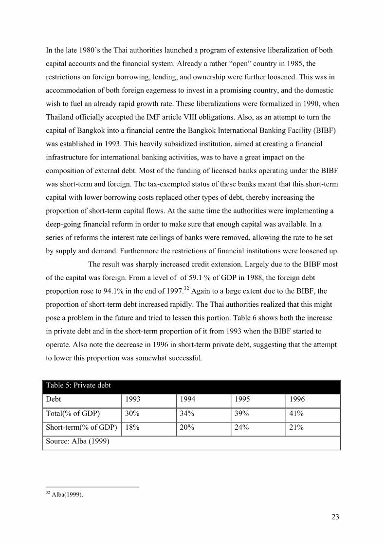
The result was sharply increased credit extension. Largely due to the BIBF most

of the capital was foreign. From a level of of 59.1 % of GDP in 1988, the foreign debt

proportion rose to 94.1% in the end of 1997.32 Again to a large extent due to the BIBF, the

proportion of short-term debt increased rapidly. The Thai authorities realized that this might

pose a problem in the future and tried to lessen this portion. Table 6 shows both the increase

in private debt and in the short-term proportion of it from 1993 when the BIBF started to

operate. Also note the decrease in 1996 in short-term private debt, suggesting that the attempt

to lower this proportion was somewhat successful.

Table 5: Private debt

Debt 1993 1994 1995 1996

Total(% of GDP) 30% 34% 39% 41%

Short-term(% of GDP) 18% 20% 24% 21%

Source: Alba (1999)

32 Alba(1999).

23

Who were the people that took these loans? Afterwards it is evident that the financial

institutions in Thailand were not prepared for the challenges of selecting and monitoring the

projects applying for loans. Evaluating the risk of potential projects as well as monitoring

these after the loan has been granted, was simply something that financial people were

inexperienced at after years of government regulations. This meant that there was a tendency

to lend money to risky businesses that were vulnerable to external shocks and perhaps also of

dubious potential productivity. Also, banks had a large willingness to take on considerable

risks. The reason for this might be the presence of what has been called “implicit guarantees”,

that is the banks assumed that the government would bail them out if they ran into trouble.

This “moral hazard” gave banks the incentive to engage in reckless lending, contributing to

the vulnerability of the situation. In addition there have been empirical studies performed in

Canada that show that competition among banks increases sharply following a deregulation of

markets33. This increased competition implies that “a typical bank extends financial services

more aggressively in the short run than it would in the long run”34. Banks simply try to

conquer parts of a newly open market as quickly as possible, expecting high revenues in the

future. Evidence in Thailand is consistent with this view. Official figures – probably

understating the true situation - suggest increased of credit extension in many traditonal high

risk sectors35. The appearence of 19 foreign banks who established themselves under the aegis

of the BIBF, further added to this process.

This lending fuelled a continuing expansion, and “expansion” often meant

acquisition of assets, especially real estate and land, which given inelastic supply meant a

sharp rise in the prices of such assets. From 1994 to 1996, fixed assets of the Thai companies

rose on average 30% per year36. This was also visible in increasing prices on the Thai stock

market. That these increases were in fact an asset bubble without stability became clear in

1996 when prices dropped suddenly - first in the real estate sector as supply exceeded

demand and tenants were becoming difficult to find. Since this led to troubles for highly debt-

levered firms the amount of non-performing loans increased. In March 1997 the size of non-

performing loans was officially 100 billion Bhats or 2.5 billion US dollars, but the true size of

“bad loans” has been estimated to three times this number.37 This fact became apparent later

as official figures set the percentage of non-performing loans to total outstanding loans at

33 Gruben et al.(1997) 34 ibid. 35 Ibid. 36 Alba(1999) 37 ibid.

24

47%38. It does seem however that the worst times for the banking sector came after the

currency crisis in June 1997, as the huge debt in foreign currency grew when the exchange

rate depreciated.

Finland39

Finland had considerable regulations of current account and financial markets before the early

80’s. Capital in- and outflows were restricted and in fact controlled by the central bank, and

interest rates were regulated at low levels. There were also considerable deposit requirements,

further slowing down the credit growth. Banks were granted tax exemptions which together

with a number of other factors - such as a small and inefficient securities market – implied

that firms to a great extent relied on the banking sector for financing. Gradually a process of

liberalization was undertaken. Restrictions on capital in- and outflows were loosened, causing

an increasing deficit in the current account as capital settled in Finland. Control over the

interest rates that banks charged was relaxed together with more lenient rules for deposits.

Banks were now freer to decide how much money to lend. While this process of liberalization

took place, there were no changes in supervision of banks and financial institutions, leaving

them a great deal of freedom to explore their new opportunities. Tighter supervision was not

introduced until 1991. For a number of years fairly unregulated banks thus operated within the

supervisional framework of regulated banks.

Following these liberalizations – which in effect were more or less completed in

1987 – the private sector started to borrow heavily. For years regulations had kept a large

demand for credit unsatisfied and now it was available in abundance. Previously the rationed

credit had been primarily allocated to the export sector. Now the sharp increase in borrowing

mainly went to households and producers for the domestic market. Households borrowed

above all in order to finance housing, while firms invested heavily. All this meant a boom in

the construction sector, a sharp increase in the pricing of land and real estate, and a large

increase in stock prices. With hindsight it is easy to see that the situation was not stable. “In

general, a bubble economy existed in Finland in the late 1980’s that was fuelled by a growing

debt burden.”40

38 Vassiliou(2001) 39 The following is based on Vihriälä(1999), and Anali et al(2002) 40 Anali et al.(2002)

25

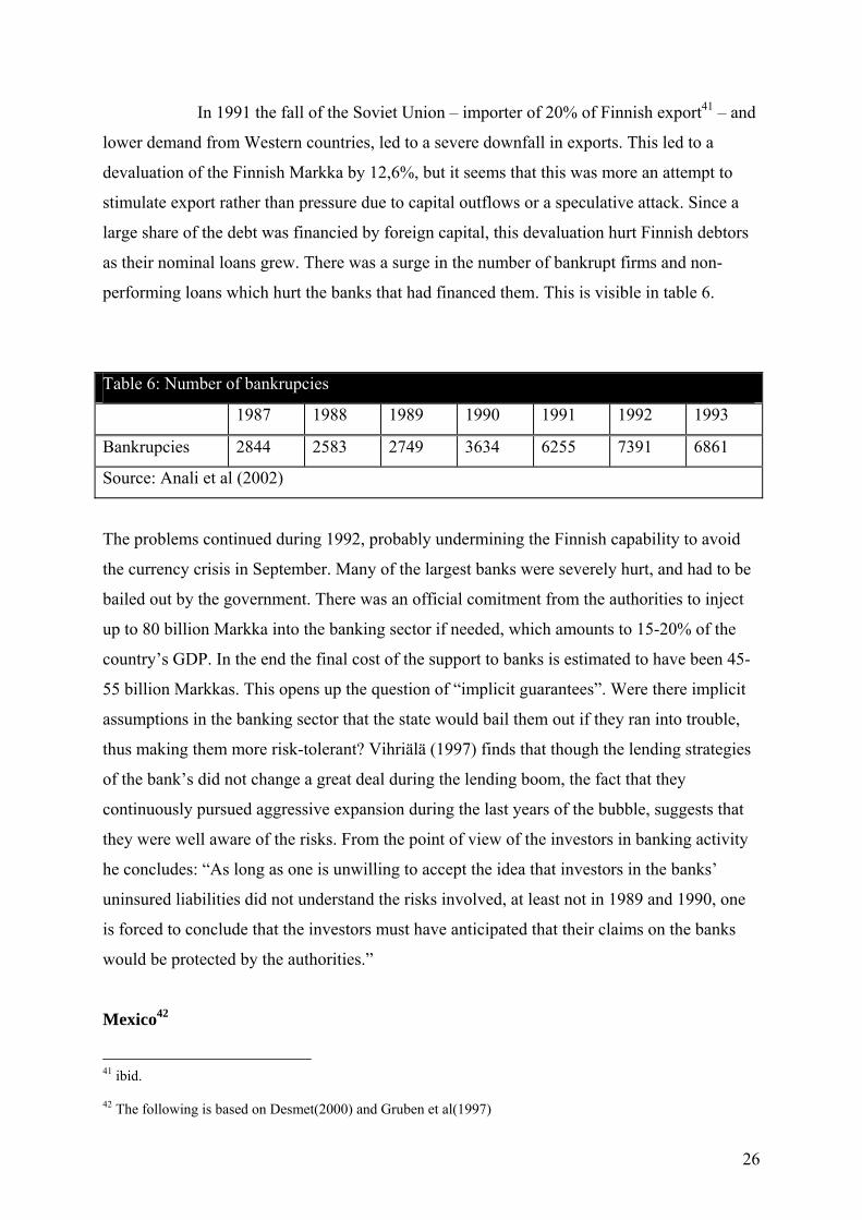
In 1991 the fall of the Soviet Union – importer of 20% of Finnish export41 – and

lower demand from Western countries, led to a severe downfall in exports. This led to a

devaluation of the Finnish Markka by 12,6%, but it seems that this was more an attempt to

stimulate export rather than pressure due to capital outflows or a speculative attack. Since a

large share of the debt was financied by foreign capital, this devaluation hurt Finnish debtors

as their nominal loans grew. There was a surge in the number of bankrupt firms and non-

performing loans which hurt the banks that had financed them. This is visible in table 6.

Table 6: Number of bankrupcies

1987 1988 1989 1990 1991 1992 1993

Bankrupcies 2844 2583 2749 3634 6255 7391 6861

Source: Anali et al (2002)

The problems continued during 1992, probably undermining the Finnish capability to avoid

the currency crisis in September. Many of the largest banks were severely hurt, and had to be

bailed out by the government. There was an official comitment from the authorities to inject

up to 80 billion Markka into the banking sector if needed, which amounts to 15-20% of the

country’s GDP. In the end the final cost of the support to banks is estimated to have been 45-

55 billion Markkas. This opens up the question of “implicit guarantees”. Were there implicit

assumptions in the banking sector that the state would bail them out if they ran into trouble,

thus making them more risk-tolerant? Vihriälä (1997) finds that though the lending strategies

of the bank’s did not change a great deal during the lending boom, the fact that they

continuously pursued aggressive expansion during the last years of the bubble, suggests that

they were well aware of the risks. From the point of view of the investors in banking activity

he concludes: “As long as one is unwilling to accept the idea that investors in the banks’

uninsured liabilities did not understand the risks involved, at least not in 1989 and 1990, one

is forced to conclude that the investors must have anticipated that their claims on the banks

would be protected by the authorities.”

Mexico42

41 ibid. 42 The following is based on Desmet(2000) and Gruben et al(1997)

26

Following troubles in the early 80’s Mexico had nationalized its banks, and imposed strict

regulations, including interest rate ceilings and dictated allocation of credit. A process of

liberalization was begun in order to increase availability of capital to speed up development.

In a number of moves leading up to re-privatization of banks in 1991, the interest rate ceilings

were abandoned, reserve deposit requirements reduced and dictated allocation eliminated. The

effects were the usual ones: foreign capital inflow, and easier access to credit leading to a

lending boom in the private sector. Again, a great deal of inflow and and domestic credit

expansion was channeled into a debt-based growth in the private sector. The total debt of the

private sector increased from the equivalent to 20% of GDP in 1989 to 55.3% in 1994.43 It has

been suggested – on good grounds – that many of the projects financed by banks were in fact

credit risks which were accepted due to aggressive lending policies. Apart from the usual

claims of implicit guarantees, Gruben et al (1997) have performed a study which concludes

that hard competition among banks was also a contributor to this. Liberalization meant the

establishment of many new banks as well as a struggle to conquer parts of a mostly new

market previously locked by regulations. This meant that banks had a tendency to follow

more short-term strategies, thereby being more risk-tolerant. Also the inexperience of the

Mexican banking system in operating in a deregulated climate, where for years investment

decisions had been dictated by the authorities, led to poor selection of projects. In relation to

this, the Mexican accounting standards were quite insufficent, masking some of the

vulnerability of the situation.

As the competitiveness of the export sector worsened, and harder times hit

Mexico, the typical problems of a highly debt-leveraged economy appeared. Bankrupted firms

led to a high degree of non-performing loans – from roughly 0% of all loans in 1990 to 8% in

late 1994.44 Already in September 1994 the government had bailed out two banks and Desmet

(2000) suggests that the expectation that further bail-outs were coming might have triggered

the currency crisis in December through increasing expected inflation. The devaluation on 20

December – an adjustment according to authorities – further increased the growth of non-

performing loans as nominal debt in foreign currency grew. Two days later the Mexican Peso

was floated after massive capital outflows. As the currency depreciated these problems

became even worse. The government finally ended up bailing out several banks.

43 Desmet(2000) 44 Ibid.

27

Sweden45

In the first part of the 1980’s, Sweden - like many other countries at this time - deregulated

the financial and banking systems. This was after decades of tight regulation, with the central

bank giving directions for banking acitivites in weekly meetings with representatives of larger

banks. Lending and interest rate ceilings together with placement requirements – a portion of

bank assets had to be in the form of government bonds with long maturity and low interest

rates – led to a situation where “banks were, in effect, transformed into repositories for

illiquid bonds, crippled in their key function in screening and monitoring loans”.46 This meant

that the banking sector had very little experience in evaluating different projects, a fact that

might have led to bad decisions in a more liberal climate. Deregulations had been resisted for

a long time, yet when the process started it proceeded with surprisingly high speed. By 1985

ceilings and placement requirement had been lifted. The effects were immediate. During the

period between 1985 and 1990 total lending by domestic institutions increased 136%.

Meanwhile an asset price bubble was forming. This was probably not triggered by the large

credit expansion since the price increases before liberalization were bigger than after. But it

still seems that the price bubble was augmented by the banks’ investment policies: “Both

inexperience in a new environment and competition among credit institutions unleashed by

deregulation played important roles in this process.”47 The stock market index rose 118%

between 1985 and 1988, and the rate of price increase of commercial real estates in

Stockholm was the highest in Europe. The first signs of troubles emerged in 1989 as rents for

housing in Stockholm were so high that tenants could not easily be found. In a year the real

estate stock price fell by 25% and in 1990 it had fallen by 52%. The troubles in the real estate

sector together with a number of external shocks – including rising interest rates – revealed

the vulnerability in the banking sector. Banks and institutions that had invested heavily in real

estate now faced problems of non-performing loans and falling stock values. Credit losses

increased, from 1% av total lending in the end of 1990 to 3,5% in 1991 and 7,5% in 1992. In

1991 two of the six biggest banks, Första Sparbanken and Nordbanken, were insolvent. The

state injected capital into Nordbanken – being one of the major owners – and guaranteed

subsidized loans to Första Sparbanken. Before the end of the bank crisis, the state had paid

out 65 billion kronor or 4-5% of GDP to the banking sector.

45 The following is based on Andersson et al(2002) and Englund(1999) 46 Englund(1999) 47 Englund(1999)

28

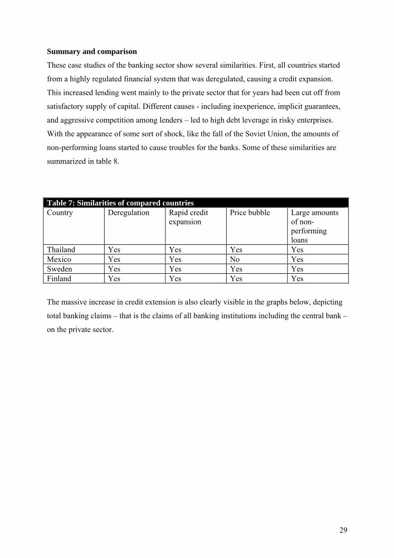
Summary and comparison

These case studies of the banking sector show several similarities. First, all countries started

from a highly regulated financial system that was deregulated, causing a credit expansion.

This increased lending went mainly to the private sector that for years had been cut off from

satisfactory supply of capital. Different causes - including inexperience, implicit guarantees,

and aggressive competition among lenders – led to high debt leverage in risky enterprises.

With the appearance of some sort of shock, like the fall of the Soviet Union, the amounts of

non-performing loans started to cause troubles for the banks. Some of these similarities are

summarized in table 8.

Table 7: Similarities of compared countries Country Deregulation Rapid credit

expansion Price bubble Large amounts

of non-performing loans

Thailand Yes Yes Yes Yes Mexico Yes Yes No Yes Sweden Yes Yes Yes Yes Finland Yes Yes Yes Yes

The massive increase in credit extension is also clearly visible in the graphs below, depicting

total banking claims – that is the claims of all banking institutions including the central bank –

on the private sector.

29

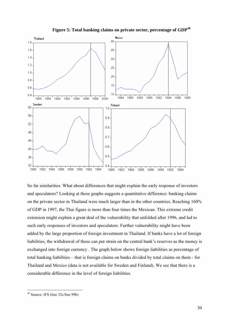
Figure 5: Total banking claims on private sector, percentage of GDP48

So far similarities. What about differences that might explain the early response of investors

and speculators? Looking at these graphs suggests a quantitative difference: banking claims

on the private sector in Thailand were much larger than in the other countries. Reaching 160%

of GDP in 1997, the Thai figure is more than four times the Mexican. This extreme credit

extension might explain a great deal of the vulnerability that unfolded after 1996, and led to

such early responses of investors and speculators. Further vulnerability might have been

added by the large proportion of foreign investment in Thailand. If banks have a lot of foreign

liabilities, the withdrawal of these can put strain on the central bank’s reserves as the money is

exchanged into foreign currency . The graph below shows foreign liabilities as percentage of

total banking liabilities – that is foreign claims on banks divided by total claims on them - for

Thailand and Mexico (data is not available for Sweden and Finland). We see that there is a

considerable difference in the level of foreign liabilities.

48 Source: IFS (line 32c/line 99b)

30

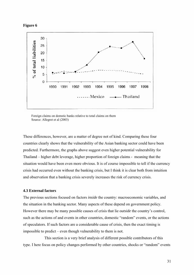
Figure 6

Foreign claims on domstic banks relative to total claims on them

Source: Allegret et al (2003)

These differences, however, are a matter of degree not of kind. Comparing these four

countries clearly shows that the vulnerability of the Asian banking sector could have been

predicted. Furthermore, the graphs above suggest even higher potential vulnerability for

Thailand – higher debt leverage, higher proportion of foreign claims - meaning that the

situation would have been even more obvious. It is of course impossible to tell if the currency

crisis had occurred even without the banking crisis, but I think it is clear both from intuition

and observation that a banking crisis severely increases the risk of currency crisis.

4.3 External factors

The previous sections focused on factors inside the country: macroeconomic variables, and

the situation in the banking sector. Many aspects of these depend on government policy.

However there may be many possible causes of crisis that lie outside the country’s control,

such as the actions of and events in other countries, domestic “random” events, or the actions

of speculators. If such factors are a considerable cause of crisis, then the exact timing is

impossible to predict – even though vulnerability to them is not.

This section is a very brief analysis of different possible contributors of this

type. I here focus on policy changes performed by other countries, shocks or “random” events

31

that might cause capital flight, and the role of large speculators. Once more the countries

discussed are Thailand, Finland, Mexico, and Sweden. It should be noted that none of the

events discussed below could possibly cause a crisis in themselves. But together with

vulnerability visible in macroeconomic variables and/or the banking sector, they might well

become the igniting spark that sets off the fire.

Policy changes in other countries

The ERM-crisis in Europe in 1992, the Mexican in 1994-1995, and the Asian in 1997 all

share one common denominator: the countries’ exchange rates were to some extent pegged to

the currency of a country that prior to the crisis began to pursue a restrictive monetary policy.

In Europe the German unification 1989 led the government to follow a path of large fiscal

spendings.49 The effects of this were resisted by the German central bank which pursued

restrictive monetary policies. Interest rates were raised and capital started to flow to Germany

from other European countries. To maintain their pegs in the long run these countries would

have to raise their interest rates as well. But given domestic problems of varying degrees,

could the countries really afford to do so if the pressure kept growing? The speculators

presumely did not think so and launched their attacks. In the Swedish and Finnish cases the

problems in the banking sector might have strenghtened this suspicion.

In Mexico the peg (de facto) was against the US dollar.50 There were large

inflows of capital, much of it in dollar-denominated bonds with short maturity. In this

situation “unfortunately for Mexico, contractionary monetary policies began in the US in

February 1994, which were reciprocated in the other hard-currency money centers.”51 This

meant that the flow of foreign investment into Mexico “could not be sustained”52 at the same

time as the peso followed the dollar’s appreciation. Capital already in Mexico furthermore,

should have been more prone to slip away in order to benefit from high interest rates in these

hard-currencies centers.

This same contractionary policy in the US was to cause troubles for the Asian

countries. Most of these countries had pegs to the dollar and had copied the Thai strategy for

attracting large amounts of foreign capital, which in effect meant that it was very easy for

investors to convert local currencies for dollars. Thus the US monetary policy should not just

49 Saxena(1996) 50 Reinhart et al.(2002) 51 Allen(1999) 52 ibid.

32

have been a cause of the creeping real appreciation of Asian currencies, but also served as an

incentive to shift investments to the US.

All three of these crisis were thus in some way connected to restrictive monetary

policies in another country. This suggests a moral dilemma: is a country responsible for the

effects of its monetary policies in other parts of the world? Delving into this is of course not

possible here.

“Random” events

Here the cases of Sweden and Finland might not be of use as reference points. Throughout

this paper there has always been an assumption that emerging market countries are more

vulnerable than established ones. The assasinations of Swedish or Finnish opposition

politicians would probably not have triggered capital outflows as it did in Mexico. Investors

simply appear to have lower confidence in the stability of developing countries and their

ability to maintain a healthy economic climate when faced with such events. Therefore I will

not go into the Scandinavian experiences.

In the first quarter of 1994 the Mexican foreign reserves were close to 30 billion

dollars.53 The country was having some internal troubles manifested in the Chiapas uprising.

Investors were concerned but not panicked by this as is evident in the following internal

memo in a “major US bank”54: “While Chiapas, in our opinion, does not pose a fundamental

threat to Mexican political stability, it is perceived to be so by many in the investment

community.” Still as the rebels achieved a symbolic victory in January 1994 by occupying the

city of San Cristobal, there were no capital outflows. On the contrary capital continued to

pour in.55 But only two months later an opposition politician was assassinated. There were

considerable capital outflows, although it is impossible to know for sure that this was really

caused by the assassination. The fixed exchange rate was maintained without greater troubles,

but foreign reserves were nearly halfed in the process: from 29.3 billion dollars in February to

16.5 billions in June undermining future ability to maintain the peg. A period of calm

followed and reserves grew somewhat. Then another assassination of an opposition politician

occurred in October, followed by suggestions that the government itself was somehow

involved. In one month the reserves fell from 17. 667 billions in October to 12. 889 in

November. Dollar-denominated bonds worth around 17 billion dollars were to mature in

53 Gruben et al. (1997) 54 Allen(1999) 55 Gruben et al.(1997)

33

1995. If all investors wanted to get out of Mexico this meant that the peg would become

impossible to maintain.

Thailand on the other hand had for long been famous for being stable. But 1996

the country was rocked by a financial scandal that cast doubts over the entire banking sector.56

One of the banks – Bangkok Bank of Commerce – was suspected of fraud.57 Investigations

revealed that banking personnel had been using bank assets for their own ends. When the

Bank of Thailand took over the bank there were no immediate consequences. But this event

hurt confidence of investors in the way the central bank – being after all supervisor of

financial activities – was running things.58 From this moment investors and speculators were

probably more attentive to what was happening in the banking sector. This occurred

simultaneously with the bursting of the asset price bubble and other problems. Still it cannot

be ruled out that these acts of a few dishonest individuals in a highly sensitive environment

acted as a catalyst or even ignition of the crisis.

Large speculators

During the Asian crisis Malaysian prime minister Mahathir more or less put the entire blame

on the irresponsible and ruthless acts of one person: speculator George Soros: “All these

countries have spent forth years to build up their economies and a moron like Soros comes

along.”59 As political as this saying might well be, it still warrants some attention. Are large

speculators not just a mechanism of currency crisis, as in the theoretical models, but also a

causing factor in themselves? Or in more specified words: can the actions of large speculators

create herding effects, inciting a flood of capital outpour as investors panic? Although

speculators have been an important assumed mechanism in all theoretical generations, little

research has been invested into the role of large players. Following accusations like that of

Mahathir, the IMF performed a study that concluded that large speculators such as Soros –

following the analogy of predators attacking a prey - were “at the rear rather then the head of

the pack”.60 Still we know that Soros was involved in the ERM crisis, and that the asset value

of his Quantum Fund increased by 25% following the fall of the British pound. With this

background, is it really believable that minor speculators and investors did not react when the

56 Andersson et al (2002) 57 Vasililou(2001) 58 Andersson et al (2002) 59 Wang(1999) 60 Corsetti(2001)

34

Quantum Fund took a short position against the Thai baht in January 1997?61 If not, to what

extent might it have influenced the chances of a crisis occuring? The study of Corsetti et al

(2001) analyzes the contention that “the activity of large players in small markets...may

trigger crises that are not justified by fundamentals, destabilizing foreign exchange and other

asset markets”.62 Although avoiding to infer too strong a role for large players, it is here still

concluded that the IMF report’s contention is not supported by actual data. On the contrary

there is nothing to contradict the assumption that the hedging funds – such as Soros’ Quantum

Fund – were key players that were the first to move and that “their presence made other

investors more aggressive in their trading strategies.” Yet I cannot see that there is really

anything supporting this claim either, so the question is still open, and the literature on this

subject still in its “infancy”.63

While it is intuitive that large players should have an impact on the chances of a

crisis occurring, it seems unlikely that are the sole underlying cause. There has to be some

sort of vulnerability that both causes traders to act and makes the country more vulnerable to

them in a feedback process.

5. Conclusion and summary This paper analyzed the possibility to predict currency crises. To this end a number of

attempts were tried and/or evaluated. First a logit model was estimated, which was unable to

explain and predict crises. This indicates that just a few variables are not enough to predict a

crisis and that more complex approaches are both justified and needed. In the next sections, a

number of possible underlying causes were analyzed using a more descriptive and qualitative

approach. The aim here was to analyze if it had been possible to predict the Asian crisis in

1997 by looking at recent history. Thus similarities within a chosen setup of countries,

Thailand – representing Asia – Finland, Sweden and Mexico were sought. First

macroeconomic fundamentals from Finland, Mexico, Sweden, and Thailand did share some

similarities. More specifically, they all had substantial or growing current account deficits,

and had suffered a loss of competitiveness in the previous 5-year period. However the main

difference was the early respone of speculators and investors in Asia following visible

problems. This suggests that there was some underlying factor not captured by macroecomic

fundamentals. I also consider banking activities in the above mentioned countries. A similar

61 ibid. 62 Ibid. 63 ibid

35

pattern emerged in all four countries. Deregulations resulted in rapid credit extension, and a

banking sector exposed to risky businesses. Harder times hurt a lot of businesses, that

damaged the banks through large amounts of non-performing loans. This situation made the

countries vulnerable to currency crises. The similarites between the different countries

suggests that it would indeed have been possible to predict that Asian countries would

become vulnerable to currency crises through an overextended banking sector. Still there was

the difference in the time it took for investors and speculators to respond. Two important

factors were the larger extent of debt leverage and large proportion of foreign debt in Asian

countries. Although it is evident that each of the analyzed countries was vulnerable, the

question about what finally triggers a crisis remains unanswered. This led to a brief discussion

about shocks and events that might intreact with vulnerability and set off a crisis. The ultimate

effect of such factors remains an open question, but they cannot be ruled out as contributors to

crisis although the contention that they are causes of crisis in themselves – that is not

interacting with inherent vulnerability – can rather safely be dismissed.

So is it possible to predict a crisis? That depends on what we mean by “predict”.

It seems that a country’s vulnerability can indeed be detected. However, there is also the

mysterious question of the triggering of the crisis. Is this deterministic? Does the vulnerability

move closer and closer to a point in time where a crisis occurs, like a branch under increased

pressure that sooner or later snaps? Or is it instead the case that vulnerability exists and some

type of event sets off the crisis? The risk of a forest fire occurring is high in a season of

drought, but it is still the careless camper that sets it off. What is the careless camper in the

case of currency crises? I would suggest that future research separates the field in two areas:

one area focusing on vulnerability and the other on the triggering. At this point I think that

vulnerability – the drought season that makes the forest highly flammable – is possible to

sense, but that the triggering factor – the careless camper - is far more elusive. That means

that predicting a crisis in the sense of specifying an exact point in time is probably impossible.

All that we can do is detect vulnerability.

36

References

Alba, P., Hernandez, L., Klingebiel, D., 1999, Financial Liberalization and the capital

account: 1988-1997, World Bank Policy Research Paper

Allegret, J., Courbis, B., Dulbecco, P., 2003, Financial liberalization and stability of the

financial system in emerging markets: the institutional dimension of financial crises, Review

of International Political Economy

Allen, R., 1999, Financial Crises and Recession in the Global Economy, Edward Elgar

Publishing, Cheltenham

Anali, A., Kolari, J., Pynnönen, S., Suvanto, A., 2002, Further evidence on the credit view:

the case of Finland, Applied Economics 34

Andersson, V., Bergman, M., 2002, Currency crisis in Sweden and Thailand – same but

different?

Breuer, J., 2004, An Exegesis on Currency and Banking Crises, Journal of Economic Surveys,

vol 18, no 3

Chui, M., 2002, Leading Indicators of Balance-of-payment Crisis: A Partial Rewiew,

Working paper no 171, Bank of England

Corsetti, G., Pesenti, P., Roubini, N., 2001, The role of large players in currency crises,

Working Paper no 8303, National Bureau of Economic Research

Desmet, K., 2000, Accounting for the Mexican banking crisis, Emerging Market Review no 1

2002

Dornbusch, R., 1997, A Thai-Mexico primer, The International Economy, September/Oktober

1997

37

Dornbusch, R., Goldfajn, I., Valdés, R., 1995, Currency crises and collaps, The Brooking

Institution

Englund, P., 1999, The Swedish banking crisis: roots and consequences, Oxford Review of

Economic Policy, vol 15, no 3

Frankel, J., Rose, A., 1996, Currency crashes in emerging markets, Working Paper no 5437,

National Bureau of Economic Research

Gillis, M., Perkins, D., Radelet, S., Roemer, M., Snodgrass, D., 2003, Economics of

Development, Norton&Company, New York

Gruben, W., McComb, R., 1997, Liberalization, Privatization, and Crash: Mexico’s Banking

System in the 1990s, Federal Reserve Bank of Dallas Economic Review

Gujarati, D., 2003, Basic Econometrics, McGraw Hill, New York

Komulainen, T., 2004, Essays on financial crises in emerging markets, Bank of Finland

Studies E.29

Kumar, M., Moorthy, U., Perraudin, W., 2003, Predicting emergent market currency crises,

Journal of Economic Finance no 10 2003

Lauridsen, L., 1998, The financial crisis in Thailand: causes, conduct, and consequences?,

World Development Report vol 26, no 8

Lim, G., Stein, J., 2004, Asian crises :theory, evidence, warning signals, CESifo working

paper no 1159

Reinhart, C., Rogoff, K., 2002, The modern history of exchange rate arrangements: a

reinterpretation, Working Paper 8963, National Bureau of Economic Research

Saxena, S., 2004, The changing nature of currency crises, Journal of Economic Surveys vol

18 no 3

38

Vassiliou, L., 2001, Legal issue: Thailand, Pricewaterhouse Coopers

Vihriälä, V., 1997, The Finnish Credit Cycle 1986-1995, Bank of Finland Studies E:7

Wang, V., 1999, Whither (or wither) the developmental state?

39

Appendix

Table 8: Descriptive statistics Developed countries Developing countries Variable Crisis Non-crisis Crisis Non-crisis

CA/GDP -0, 0189 (0, 0385)

-0,00494 (0,0338)

-0,0380 (0,0469)

-0,0324 (0,0533)

BB/GDP -0, 166 (0,0447)

-0,0323 (0,0358)

-0,0534 (0,0928)

-0,0222 (0,0516)

GAP -0,00418 (0,0230)

0,000441 (0,0223)

0,00955 (0,0397)

0,00242 (0,0303)

∆REER -0,765 (17,137)

1,300 (12,290)

-0,768 (20,367)

-2,793 (17,942)

Table 9: Countries included in discrete-choice regressions

Developing countries Developed countries

Bolivia Australia

Brazil Austria

Colombia Belgium

Ecuador Canada

Indonesia Denmark

Korea Finland

Malaysia France

Mexico Italy

Morocco Norway

Pakistan Portugal

Paraguay Spain

Phillipines Sweden

Singapore Switzerland

Thailand

Venezuela

40

41