
Predicting Component Failures at Early Design...
158
Saarland University Faculty of Natural Sciences and Technology I Department of Computer Science Master’s Program in Computer Science Master’s Thesis Predicting Component Failures at Early Design Time submitted by Melih Demir on November 17, 2006 Supervisor Prof. Dr. Andreas Zeller Advisor Thomas Zimmermann Reviewers Prof. Dr. Andreas Zeller Prof. Dr. Reinhard Wilhelm
Transcript of Predicting Component Failures at Early Design...

Saarland UniversityFaculty of Natural Sciences and Technology I
Department of Computer ScienceMaster’s Program in Computer Science
Master’s Thesis
Predicting Component Failures atEarly Design Time
submitted by
Melih Demir
on November 17, 2006
SupervisorProf. Dr. Andreas Zeller
AdvisorThomas Zimmermann
ReviewersProf. Dr. Andreas Zeller
Prof. Dr. Reinhard Wilhelm


Statement
Hereby I confirm that this thesis is my own work and that I have docu-mented all sources used.
Saarbrucken, 17.11.2006
Melih Demir


Acknowledgements
Hereby, I would like to express my gratitude to Turkish Education Foun-dation and German Academic Exchange Service. Without their financialsupport, a master’s study in Germany would have never been possible.
I’d like to thank my supervisor Prof. Andreas Zeller for his guidance, andhis inspiring courses that motivated me to work in this field. I’d also like tothank Tom Zimmermann, who has always kept an eye on the progress of mywork and guided me in every stage of my thesis.
I am thankful to Adrian Schroter, who provided me with his R-scripts andthe details of his study, both of which played an important role in the secondpart of my work. I’d like to thank Valentin Dallmeier for providing me withthe SIBRELIB library. I’d also like to thank Daniel Schreck and NicolasBettenburg for their helpful comments on the earlier versions of this thesis.
The members of the Software Engineering Chair, especially ‘Diplomanden’and ‘Mitarbeiter’ with whom I shared the same office, also contributed tomy work significantly by providing me with a friendly working atmosphere.It was a great pleasure to work within this chair.
For the acceptance to the International Max Planck Research School, whereI’ve also found a similar working environment; support; and friendship, I’mthankful to Kerstin Meyer-Ross. Being part of the IMPRS family was one ofthe most important experiences I’ve had in Germany.
I’d like to thank Prof. Reinhard Wilhelm, who has accepted to spend hisvaluable time to be the second examiner for this thesis.
Studying and living in Saarbrucken wouldn’t be possible without my friends,who have always supported and motivated me. Having them by my side, Ihave felt at home for the last two years.
My family have supported me in every moment of my life, and simple thankswould never suffice for what they’ve done.
5

6

Abstract
For the effective prevention and elimination of defects and failures in a soft-ware system, it is important to know which parts of the software are morelikely to contain errors, and therefore, can be considered as “risky”. To in-crease reliability and quality, more effort should be spent in risky componentsduring design, implementation, and testing.
Examining the version archive and the code of a large open-source project,we have investigated the relation between the risk of components as measuredby post-release failures, and different code structures; such as method calls,variables, exception handling expressions and inheritance statements. Wehave analyzed the different types of usage relations between components,and their effects on the failures. We utilized three commonly used statisticaltechniques to build failure prediction models. As a realistic opponent toour models, we introduced a “simple prediction model” which makes use ofthe riskiness information from the available components, rather than makingrandom guesses.
While the results from the classification experiments supported the use ofcode structures to predict failure-proneness, our regression analyses showedthat the design time decisions also affected component riskiness. Our modelswere able to make precise predictions, with even only the knowledge of theinheritance relations. Since inheritance relations are defined earliest at designtime; based on the results of this study, we can say that it may be possibleto initialize preventive actions against failures even early in the design phaseof a project.
7

8

Contents
1 Introduction 171.1 Risky Components . . . . . . . . . . . . . . . . . . . . . . . . 181.2 What We Can Do . . . . . . . . . . . . . . . . . . . . . . . . . 191.3 How to Proceed . . . . . . . . . . . . . . . . . . . . . . . . . . 21
2 Related Work 222.1 Faults or Failures? . . . . . . . . . . . . . . . . . . . . . . . . 222.2 Related Work . . . . . . . . . . . . . . . . . . . . . . . . . . . 23
2.2.1 Software Metrics . . . . . . . . . . . . . . . . . . . . . 232.2.2 Project History . . . . . . . . . . . . . . . . . . . . . . 292.2.3 Software Repositories . . . . . . . . . . . . . . . . . . . 31
A Tokens and Risk Classes 36
3 Initial Hypothesis 37
4 Collecting Data 404.1 Project under Inspection . . . . . . . . . . . . . . . . . . . . . 404.2 Determining Failure-Prone Entities . . . . . . . . . . . . . . . 41
4.2.1 CVS and Bugzilla . . . . . . . . . . . . . . . . . . . . . 414.2.2 Modified Entities . . . . . . . . . . . . . . . . . . . . . 424.2.3 Searching Problem Reports for Failures . . . . . . . . . 434.2.4 Matching Changes and Failures . . . . . . . . . . . . . 454.2.5 Defective/Failure-Prone Entities . . . . . . . . . . . . . 45
4.3 Token Information . . . . . . . . . . . . . . . . . . . . . . . . 46
5 Preliminaries 515.1 Statistical Methods . . . . . . . . . . . . . . . . . . . . . . . . 51
5.1.1 Linear Regression . . . . . . . . . . . . . . . . . . . . . 515.1.2 Logistic Regression . . . . . . . . . . . . . . . . . . . . 54
9

5.1.3 Support Vector Machines . . . . . . . . . . . . . . . . . 565.2 Evaluating Model Accuracy . . . . . . . . . . . . . . . . . . . 61
6 Classification Models and Results 636.1 R System . . . . . . . . . . . . . . . . . . . . . . . . . . . . . 636.2 Input Format . . . . . . . . . . . . . . . . . . . . . . . . . . . 636.3 Joining Failure and Token Information . . . . . . . . . . . . . 646.4 Token Groups . . . . . . . . . . . . . . . . . . . . . . . . . . . 666.5 Random Classifier . . . . . . . . . . . . . . . . . . . . . . . . . 686.6 Building Classification Models . . . . . . . . . . . . . . . . . . 696.7 Results from Classification Models . . . . . . . . . . . . . . . 69
6.7.1 Cross-Validation Experiments . . . . . . . . . . . . . . 706.7.2 Complement Method Experiments . . . . . . . . . . . . 72
6.8 Conclusion . . . . . . . . . . . . . . . . . . . . . . . . . . . . . 73
B Usage Relations and Failures 75
7 Revised Hypothesis 767.1 Design Time Relations and Failures . . . . . . . . . . . . . . . 767.2 Design Evolution . . . . . . . . . . . . . . . . . . . . . . . . . 777.3 Revised Hypothesis . . . . . . . . . . . . . . . . . . . . . . . . 80
8 Tokens for Usage Relations & Further Failure Mappings 828.1 Tokens for Usage Relations . . . . . . . . . . . . . . . . . . . . 828.2 More Components with Failures . . . . . . . . . . . . . . . . . 85
9 Regression Models and Results 909.1 Differences in Input . . . . . . . . . . . . . . . . . . . . . . . . 90
9.1.1 Failure Counts as Dependent Variable . . . . . . . . . . 909.1.2 Inputs at Fine and Coarse Granularities . . . . . . . . 919.1.3 Excluding Project Independent Classes . . . . . . . . . 93
9.2 Differences in Evaluation . . . . . . . . . . . . . . . . . . . . . 949.2.1 Random Splitting and Complement Method . . . . . . 949.2.2 Riskiness Rankings . . . . . . . . . . . . . . . . . . . . 959.2.3 Simple Prediction Model . . . . . . . . . . . . . . . . . 97
9.3 Building Regression Models . . . . . . . . . . . . . . . . . . . 999.4 Results from Regression Experiments . . . . . . . . . . . . . . 99
9.4.1 Files as Instances and Classes as Features . . . . . . . 1009.4.2 Files as Instances and Packages as Features . . . . . . 1059.4.3 Packages as Instances and Classes as Features . . . . . 108
10

9.4.4 Packages as Instances and Packages as Features . . . . 1149.4.5 Comparison of Methods . . . . . . . . . . . . . . . . . 117
9.5 Usage Relations: General or Detailed? . . . . . . . . . . . . . 1219.6 Conclusion . . . . . . . . . . . . . . . . . . . . . . . . . . . . . 122
10 Conclusion and Future Work 12510.1 Conclusion . . . . . . . . . . . . . . . . . . . . . . . . . . . . . 12510.2 Future Work . . . . . . . . . . . . . . . . . . . . . . . . . . . . 126
A Regression Experiments Results 128A.1 Linear Regression Models . . . . . . . . . . . . . . . . . . . . 129A.2 Support Vector Machines Models . . . . . . . . . . . . . . . . 137A.3 Simple Prediction Models . . . . . . . . . . . . . . . . . . . . 145
Bibliography 153
11
List of Figures
1.1 Our Failure-Proneness Prediction Method . . . . . . . . . . . 21
4.1 Effects of Changes on Entities . . . . . . . . . . . . . . . . . . 43
5.1 Linear Least Squares Fitting in R2 . . . . . . . . . . . . . . . 535.2 Logit Function . . . . . . . . . . . . . . . . . . . . . . . . . . 545.3 Logistic Regression Function . . . . . . . . . . . . . . . . . . . 555.4 Separating Hyperplanes . . . . . . . . . . . . . . . . . . . . . 565.5 Support Vectors and Maximum Margin Hyperplane . . . . . . 565.6 Transformation from Instance Space to Feature Space . . . . . 585.7 10-Fold Cross Validation . . . . . . . . . . . . . . . . . . . . . 615.8 Complement Method . . . . . . . . . . . . . . . . . . . . . . . 61
6.1 Classification Experiments Input Format . . . . . . . . . . . . 646.2 Joining Failure and Token Databases . . . . . . . . . . . . . . 656.3 Precision-Recall Values from Cross-Validation Experiments . . 716.4 Precision-Recall Values from Complement Experiments . . . . 71
8.1 Different Levels of Usage Relations . . . . . . . . . . . . . . . 848.2 Mapping Failures to Correct Releases . . . . . . . . . . . . . . 868.3 Failure Frequencies in Eclipse Release 2.0 - Initial Mappings . 888.4 Failure Frequencies in Eclipse Release 2.0 - Improved Mappings 888.5 Failure Frequencies in Eclipse Release 2.1 - Initial Mappings . 898.6 Failure Frequencies in Eclipse Release 2.1 - Improved Mappings 89
9.1 Regression Experiments Input Format . . . . . . . . . . . . . 919.2 Overestimation of Number of Failures in Packages . . . . . . . 929.3 Data Splitting Combined with Complement Method . . . . . . 959.4 Simple Prediction Model Example . . . . . . . . . . . . . . . . 989.5 Precision-Recall Values for Linear Regression Models (Instances:
Files, Features: Classes) . . . . . . . . . . . . . . . . . . . . . 1019.6 Precision-Recall Values for SVM Models (Instances: Files,
Features: Classes) . . . . . . . . . . . . . . . . . . . . . . . . . 102
12

9.7 Precision-Recall Values for Simple Prediction Models (Instances:Files, Features: Classes) . . . . . . . . . . . . . . . . . . . . . 104
9.8 Precision-Recall Values for Linear Regression Models (Instances:Files, Features: Packages) . . . . . . . . . . . . . . . . . . . . 106
9.9 Precision-Recall Values for SVM Models (Instances: Files,Features: Packages) . . . . . . . . . . . . . . . . . . . . . . . . 107
9.10 Precision-Recall Values for Simple Prediction Models (Instances:Files, Features: Packages) . . . . . . . . . . . . . . . . . . . . 109
9.11 Precision-Recall Values for Linear Regression Models (Instances:Packages, Features: Files) . . . . . . . . . . . . . . . . . . . . 110
9.12 Precision-Recall Values for SVM Models (Instances: Packages,Features: Files) . . . . . . . . . . . . . . . . . . . . . . . . . . 112
9.13 Precision-Recall Values for Simple Prediction Models (Instances:Packages, Features: Files) . . . . . . . . . . . . . . . . . . . . 113
9.14 Precision-Recall Values for Linear Regression Models (Instances:Packages, Features: Packages) . . . . . . . . . . . . . . . . . . 115
9.15 Precision-Recall Values for SVM Models (Instances: Packages,Features: Packages) . . . . . . . . . . . . . . . . . . . . . . . . 116
9.16 Precision-Recall Values for Simple Prediction Models (Instances:Packages, Features: Packages) . . . . . . . . . . . . . . . . . . 118
9.17 Comparison of Regression Models (Instances: Files, Features:Classes) . . . . . . . . . . . . . . . . . . . . . . . . . . . . . . 119
9.18 Comparison of Regression Models (Instances: Packages, Fea-tures: Classes) . . . . . . . . . . . . . . . . . . . . . . . . . . . 120
9.19 Comparison of Regression Models (Instances: Packages, Fea-tures: Packages) . . . . . . . . . . . . . . . . . . . . . . . . . . 121
13

List of Tables
2.1 Summary of Related Studies without Historical Data . . . . . 342.2 Summary of Related Studies with Historical Data . . . . . . . 35
4.1 Eclipse Project Failure History . . . . . . . . . . . . . . . . . . 444.2 HelloWorld.java Source File . . . . . . . . . . . . . . . . . . . 464.3 Possible AST for HelloWorld.java File (Without Method Body) 474.4 Possible AST for HelloWorld.java File (Method Body) . . . . 484.5 Tokens for HelloWorld.java at Source File Level . . . . . . . . 50
5.1 Summary of Statistical Methods . . . . . . . . . . . . . . . . . 605.2 Correspondence of Real and Predicted Results . . . . . . . . . 62
6.1 Number of Instances in Token Groups under Examination . . 67
7.1 AntCorePlugin.java Source File from the Eclipse Project . . . 78
8.1 Tokens in AntCorePlugin.java Source File . . . . . . . . . . . 838.2 Number of Files with At Least One Failure . . . . . . . . . . . 87
9.1 Distribution of Normal & Filtered Tokens in Eclipse Release 2.0 939.2 Rank Correlation Example . . . . . . . . . . . . . . . . . . . . 969.3 Spearman, Top-5% Spearman, and Top-5% Precision Values
for Linear Regression Models (Instances: Files, Features: Classes)1019.4 Spearman, Top-5% Spearman, and Top-5% Precision Values
for SVM Models (Instances: Files, Features: Classes) . . . . . 1029.5 Spearman, Top-5% Spearman, and Top-5% Precision Values
for Simple Prediction Models (Instances: Files, Features: Classes)1049.6 Spearman, Top-5% Spearman, and Top-5% Precision Values
for Linear Regression Models (Instances: Files, Features: Pack-ages) . . . . . . . . . . . . . . . . . . . . . . . . . . . . . . . . 106
9.7 Spearman, Top-5% Spearman, and Top-5% Precision Valuesfor SVM Models (Instances: Files, Features: Packages) . . . . 107
14

9.8 Spearman, Top-5% Spearman, and Top-5% Precision Valuesfor Simple Prediction Models (Instances: Files, Features: Pack-ages) . . . . . . . . . . . . . . . . . . . . . . . . . . . . . . . . 109
9.9 Spearman, Top-5% Spearman, and Top-5% Precision Valuesfor Linear Regression Models (Instances: Packages, Features:Files) . . . . . . . . . . . . . . . . . . . . . . . . . . . . . . . . 110
9.10 Spearman, Top-5% Spearman, and Top-5% Precision Valuesfor SVM Models (Instances: Packages, Features: Files) . . . . 112
9.11 Spearman, Top-5% Spearman, and Top-5% Precision Valuesfor Simple Prediction Models (Instances: Packages, Features:Files) . . . . . . . . . . . . . . . . . . . . . . . . . . . . . . . . 113
9.12 Spearman, Top-5% Spearman, and Top-5% Precision Valuesfor Linear Regression Models (Instances: Packages, Features:Packages) . . . . . . . . . . . . . . . . . . . . . . . . . . . . . 115
9.13 Spearman, Top-5% Spearman, and Top-5% Precision Valuesfor SVM Models (Instances: Packages, Features: Packages) . . 116
9.14 Spearman, Top-5% Spearman, and Top-5% Precision Valuesfor Simple Prediction Models (Instances: Packages, Features:Packages) . . . . . . . . . . . . . . . . . . . . . . . . . . . . . 118
A.1 Results of Linear Regression Models - Release 2.0 Testing Data- Instances: Files, Features: Classes . . . . . . . . . . . . . . . 129
A.2 Results of Linear Regression Models - Release 2.1 Testing Data- Instances: Files, Features: Classes . . . . . . . . . . . . . . . 130
A.3 Results of Linear Regression Models - Release 2.0 Testing Data- Instances: Files, Features: Packages . . . . . . . . . . . . . . 131
A.4 Results of Linear Regression Models - Release 2.1 Testing Data- Instances: Files, Features: Packages . . . . . . . . . . . . . . 132
A.5 Results of Linear Regression Models - Release 2.0 Testing Data- Instances: Packages, Features: Classes . . . . . . . . . . . . . 133
A.6 Results of Linear Regression Models - Release 2.1 Testing Data- Instances: Packages, Features: Classes . . . . . . . . . . . . . 134
A.7 Results of Linear Regression Models - Release 2.0 Testing Data- Instances: Packages, Features: Packages . . . . . . . . . . . . 135
A.8 Results of Linear Regression Models - Release 2.1 Testing Data- Instances: Packages, Features: Packages . . . . . . . . . . . . 136
A.9 Results of Support Vector Machines Models - Release 2.0 Test-ing Data - Instances: Files, Features: Classes . . . . . . . . . . 137
A.10 Results of Support Vector Machines Models - Release 2.1 Test-ing Data - Instances: Files, Features: Classes . . . . . . . . . . 138
15
A.11 Results of Support Vector Machines Models - Release 2.0 Test-ing Data - Instances: Files, Features: Packages . . . . . . . . . 139
A.12 Results of Support Vector Machines Models - Release 2.1 Test-ing Data - Instances: Files, Features: Packages . . . . . . . . . 140
A.13 Results of Support Vector Machines Models - Release 2.0 Test-ing Data - Instances: Packages, Features: Classes . . . . . . . 141
A.14 Results of Support Vector Machines Models - Release 2.1 Test-ing Data - Instances: Packages, Features: Classes . . . . . . . 142
A.15 Results of Support Vector Machines Models - Release 2.0 Test-ing Data - Instances: Packages, Features: Packages . . . . . . 143
A.16 Results of Support Vector Machines Models - Release 2.1 Test-ing Data - Instances: Packages, Features: Packages . . . . . . 144
A.17 Results of Simple Prediction Models - Release 2.0 Testing Data- Instances: Files, Features: Classes . . . . . . . . . . . . . . . 145
A.18 Results of Simple Prediction Models - Release 2.1 Testing Data- Instances: Files, Features: Classes . . . . . . . . . . . . . . . 146
A.19 Results of Simple Prediction Models - Release 2.0 Testing Data- Instances: Files, Features: Packages . . . . . . . . . . . . . . 147
A.20 Results of Simple Prediction Models - Release 2.1 Testing Data- Instances: Files, Features: Packages . . . . . . . . . . . . . . 148
A.21 Results of Simple Prediction Models - Release 2.0 Testing Data- Instances: Packages, Features: Classes . . . . . . . . . . . . . 149
A.22 Results of Simple Prediction Models - Release 2.1 Testing Data- Instances: Packages, Features: Classes . . . . . . . . . . . . . 150
A.23 Results of Simple Prediction Models - Release 2.0 Testing Data- Instances: Packages, Features: Packages . . . . . . . . . . . . 151
A.24 Results of Simple Prediction Models - Release 2.1 Testing Data- Instances: Packages, Features: Packages . . . . . . . . . . . . 152
16

Chapter 1
Introduction
According to a market research report [18] from 2004, the number of comput-ers-in-use worldwide in 2005 was estimated to be 938 million, whereas thisnumber was expected to reach to 1.6 billion by 2010. Today, computers areintrinsic parts of almost every industry, ranging from telecommunications tomedical research. As the programs that control the functioning of computersand enable them to perform specific tasks, software is an indispensable partof computers, and our daily lives as well.
With the rapid increase in computer use, software development has becomea big industry. In this growing market, where the total software sales werereported to have reached up to $180 billion in 2000 [51], software developmentcompanies are always in competition. One of the key factors that determinewhether a software project will be successful is quality, and every softwarecompany tries to provide its customers with high quality software. Withsoftware becoming more and more crucial to the operation of the systems onwhich we depend, as a part of the quality expectations, users and projectmanagers expect their software to have reliability, the ability of a systemto perform its required functions under specified conditions for a specifiedperiod of time [13].
During the software development process, developers try to increase reliabil-ity by eliminating the errors inside the programs with the help of activitiessuch as reviews and testing. Despite all efforts, some errors may still remainin the product, and they are discovered later by the users, as they experi-ence failures. In addition to user dissatisfaction, software failures may causeexpensive or unrecoverable damages:
17

• Therac-25, a radiation therapy machine, was involved between 1985and 1987 in at least six known accidents in which patients were givenmassive overdoses of radiation due to “software errors” [35]. At leastfive patients died of the overdoses.
• In 2003, a local outage that went undetected due to a “race condi-tion” [45] in General Electric Energy’s monitoring software caused apower-outage in North America, affecting 10 million people in Canadaand 40 million people in the U.S.A., with an estimated financial loss of$6 billion [22].
• According to a federal study [51], the cost of software failures to theU.S. economy was estimated to be around $60 billion annually.
1.1 Risky Components
With our increasing dependency on computers and software, our vulnerabilityto the damages caused by software failures is also increasing. In order toavoid software failures and such damages, and to deliver reliable softwareto customers, developers have to spend more effort on software projects.However, providing reliability via debugging, verification, and testing mayalready take between 50% and 70% of the total development costs [24], andany extra work to improve reliability would naturally increase this rate. Withthe additional care taken in order not to introduce defects into the system inthe first place, the time spent on the individual elements of a project wouldalso increase. Under these circumstances, the additional time and resourcesneeded to prevent and eliminate defects may become as questionable as thedamages that might be caused by the failures.
With the problems described above, the knowledge about the parts of thesoftware which are more open to errors, the elements which may cause morefailures than others, and the number of such failure-prone components in thesystem becomes more valuable than ever. The managers’ ability to makebetter decisions about how to allocate the available resources depends onthis knowledge. Such information also enables an optimal distribution ofthe developer’s time and effort to the problematic parts of the system, fromwhich the developers would definitely profit.
Taking these issues into consideration, in this study, we tried to help the man-agers and developers by estimating the failure-proneness of software compo-nents, and detecting those parts of software systems which need more effort.
18

We focused our attention on the post-release failures because it takes moretime to correct these failures [29], resulting in higher costs, and the users aremore concerned about the number of post-release failures.
We believe that the large number of post-release failures detected in a com-ponent may be explained by either the component’s high cognitive complex-ity [7], or the problems in the development process. The cognitive complexityof a component, in other words, the mental burden of the individuals whohave to deal with that part of the system, explains how difficult it would befor the developers to understand, realize, and verify the requirements or thefunctionality of that component. Components with high cognitive complex-ity would be more difficult to design, implement, test, and maintain; andtherefore more likely to contain defects and cause failures.
Identification of those complex components, which which we also call asrisky components due to their complex nature and openness to errors, beforethe deployment of the product (preferably at the earlier stages) would helpplanning the execution of development activities; increase quality; and finallysave money, time, and work. Having such an identification available at thedesign phase of the project, developers can carefully reconsider the designdecisions, evaluate the gains brought by the use of different alternatives, andtake extra caution for the risky components for which no alternatives exist.During implementation, programmers with more experience may be given thetask of coding risky components, and these components can also be testedmore thoroughly.
At this point, one can argue that high rates of post-release failures in thecomponents of a system may also be explained by some inefficiencies in thedevelopment process, such as inappropriate methods and tools used. Failurescaused by these problems may not be simply solved by redesign, refactoring,or more testing. However, such problems tend to affect the whole system,and if many components are determined to be risky in a project, then thequality of the development process would also be questioned and improvedin the necessary areas.
1.2 What We Can Do
In order to determine the risky components, software code may be an im-portant source of information. The relation between defects and specific
19
properties of program code was examined by researchers. Earlier studiesaimed to determine and validate software metrics which may be useful tocapture the software complexity, and predict software defects. While severalstudies [5, 10, 16, 17, 33, 38, 40, 41] have shown that metrics such as thelength of code or McCabe complexity metric had high correlations with thenumber of defects; still, there exists no single set of metrics that is successfulat predicting failures or defects in all projects [40]. The (in)applicability ofproposed metrics to the project at hand also plays an important role in thisissue.
When available, software repositories may also be a valuable data source forpredicting failures. Combining the information contained in version controlarchives and bug tracking systems, the number of failures associated witheach component can be determined [12, 23, 36, 39, 47, 49]. Version controlsystems also provide researchers with vast amount of information about howa system evolves [25, 42, 43, 53]. Using the information from these sources,models to predict the failures in the later releases can be built. However,the long history data needed for stable and accurate models might not beavailable in new projects, or for the components under inspection.
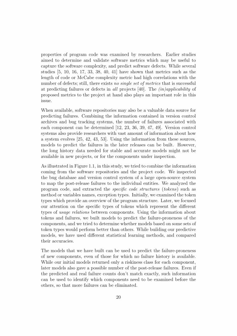
As illustrated in Figure 1.1, in this study, we tried to combine the informationcoming from the software repositories and the project code. We inspectedthe bug database and version control system of a large open-source systemto map the post-release failures to the individual entities. We analyzed theprogram code, and extracted the specific code structures (tokens) such asmethod or variables names, exception types. Initially, we examined the tokentypes which provide an overview of the program structure. Later, we focusedour attention on the specific types of tokens which represent the differenttypes of usage relations between components. Using the information abouttokens and failures, we built models to predict the failure-proneness of thecomponents, and we tried to determine whether models based on some sets oftoken types would perform better than others. While building our predictivemodels, we have used different statistical learning methods, and comparedtheir accuracies.
The models that we have built can be used to predict the failure-pronenessof new components, even of those for which no failure history is available.While our initial models returned only a riskiness class for each component,later models also gave a possible number of the post-release failures. Even ifthe predicted and real failure counts don’t match exactly, such informationcan be used to identify which components need to be examined before theothers, so that more failures can be eliminated.
20

Figure 1.1: Our Failure-Proneness Prediction Method
1.3 How to Proceed
This thesis explains the details of our study, and is organized in the followingway: First we take a look at the earlier work from the field in Chapter 2.In the following chapter, our initial research hypothesis and contributions ofour study are presented. Chapter 4 explains the system under inspection andhow we can collect the necessary token and failure information from projectdatabases and code. This information is used to build the models usingstatistical methods, the basics of which are given in Chapter 5. In Chapter 6we discuss about the results from classification models, which resulted in ourrevised hypothesis, explained in Chapter 7. Chapter 8 describes how thedata required for the second group of models is collected, and in Chapter 9,we demonstrate the results from the experiments with these models. In thefinal chapter, we draw some conclusions about our complete work and presentideas about further studies.
21

Chapter 2
Related Work
In this chapter, we would like to make a summary of the studies conductedby other researchers in this field. However, before we start describing thesestudies, we would like to clarify the definitions of some terms which havebeen used interchangeably in different studies.
2.1 Faults or Failures?
The terms, bug, fault, defect and failure, have been often used in manystudies, with varying meanings. In our study, we followed the definitionsfrom Zeller [55] for the given terms: A defect, also known as a bug or fault,is an error in the program code. On the other hand, a failure is an externallyobservable error in the program behavior.
For a failure to come into being, initially, a defect has to be created in theprogram code by the programmer. When the defective code is executed undercertain circumstances, it causes an error in the program state, which is calledan infection. As the program execution continues, this infection propagates,and causes further infections, creating an infection chain. Finally, one of theinfections in this chain causes the failure.
Not every defect results in an infection, and not every infection results in afailure. The defective code has to be executed under the circumstances inwhich the infection occurs; and an infection may be overwritten, masked, oreven corrected during the program run. However, every failure is caused by
22
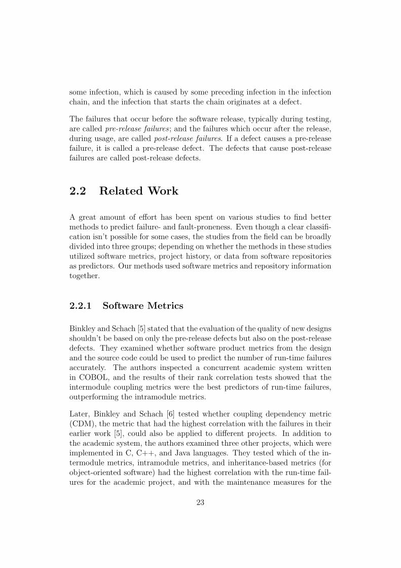
some infection, which is caused by some preceding infection in the infectionchain, and the infection that starts the chain originates at a defect.
The failures that occur before the software release, typically during testing,are called pre-release failures; and the failures which occur after the release,during usage, are called post-release failures. If a defect causes a pre-releasefailure, it is called a pre-release defect. The defects that cause post-releasefailures are called post-release defects.
2.2 Related Work
A great amount of effort has been spent on various studies to find bettermethods to predict failure- and fault-proneness. Even though a clear classifi-cation isn’t possible for some cases, the studies from the field can be broadlydivided into three groups; depending on whether the methods in these studiesutilized software metrics, project history, or data from software repositoriesas predictors. Our methods used software metrics and repository informationtogether.
2.2.1 Software Metrics
Binkley and Schach [5] stated that the evaluation of the quality of new designsshouldn’t be based on only the pre-release defects but also on the post-releasedefects. They examined whether software product metrics from the designand the source code could be used to predict the number of run-time failuresaccurately. The authors inspected a concurrent academic system writtenin COBOL, and the results of their rank correlation tests showed that theintermodule coupling metrics were the best predictors of run-time failures,outperforming the intramodule metrics.
Later, Binkley and Schach [6] tested whether coupling dependency metric(CDM), the metric that had the highest correlation with the failures in theirearlier work [5], could also be applied to different projects. In addition tothe academic system, the authors examined three other projects, which wereimplemented in C, C++, and Java languages. They tested which of the in-termodule metrics, intramodule metrics, and inheritance-based metrics (forobject-oriented software) had the highest correlation with the run-time fail-ures for the academic project, and with the maintenance measures for the
23

other three projects. According to the rank correlation values, CDM had thehighest correlation in three projects, and was ranked second in the remain-ing case. These results supported the idea that CDM could be used for theprediction of failure-prone modules in other projects.
Fenton and Ohlsson [21] conducted a quantitative study of faults and fail-ures in two releases of a major commercial system, and aimed to provideevidence for/against some ‘common wisdom’. While their results providedsome support for the Pareto principle of small number of modules containingthe faults that cause the most failures, the authors rejected the hypothesisthat the modules with those faults constitute most of the code size. Unlikemany other studies, for the system at hand, the authors strongly rejectedthe hypothesis that a higher incidence of faults in pre-release testing implieshigher incidence of failures in the operations. The authors also found weaksupport for that, the predictions based on simple size metrics such as linesof code (LOC) were better. Fenton and Ohlsson weakly rejected the superi-ority of the complexity metrics against the simple size metrics at predictingfailure-prone modules. The hypothesis that fault densities remain constantbetween subsequent major releases of a system at the corresponding phasesof testing and operation was partly supported.
Nagappan et al. [41] also worked on software metrics, and they aimed toconstruct and validate a set of easy-to-measure in-process metrics that can beused to predict the field quality, determined by the number of failures foundby customers. The authors constructed multiple linear regression modelson the principal components of the metrics from their STREW-J metricsuite. The authors collected the metrics from 22 academic projects, and theyevaluated the accuracy of their models using random splitting, an evaluationtechnique in which the training and testing sets are formed by random splits.In order to assess whether the metrics data could be used for classificationpurposes, the authors also built binary logistic models that identified thehigh and low quality projects. The results of the regression and classificationtests showed that the models based on the metrics data performed well forpredicting post-release failures and identifying low quality projects.
In a later study conducted at Microsoft Research, Nagappan and Ball [38]inspected whether the static analysis defect density, the number of defectsfound by static analysis tools per thousands of line of code (KLOC), couldbe used as a predictor of pre-release defect density. They used the resultsof the analyses made by Microsoft’s PREfix and PREfast tools on WindowsServer 2003 as input, and performed regression analyses and correlation tests.Like in the earlier study conducted by Nagappan et al.[41], the authors also
24

applied the random splitting technique to evaluate the predictive accuracy oftheir models. To classify components as fault-prone and not fault-prone, theyused discriminant analysis instead of binary logistic models. Their resultsshowed that static analysis defect density was a good predictor of pre-releasedefect density.
Continuing the studies on Microsoft projects, Nagappan et al. [40] usedsoftware archives to map post-release failures to individual modules of fiveprojects, and computed standard complexity metrics for these modules. Con-sidering that each defect is discovered after a failure is detected, the authorstook the likelihood of a post-release defect in some entity as the likelihoodof detecting at least one post-release failure, and they tested whether anyof examined metrics would correlate with the post-release defects. Althoughsome metrics correlated with the defects in each of the five projects, therewas no single metric which worked best in all projects. Later, the authorsalso combined their metrics by using principal component analysis (PCA),and the regression models built on the resulting principal components weresuccessful at estimating the defects, when the project data was separatedinto training and testing sets by using random-splitting. The experimentsalso showed that the prediction models built on the data from one projectcould be used on similar projects.
Khoshgoftaar et al. [33] used a large set of metrics composed of process, prod-uct, and execution metrics in order to classify the modules in four consec-utive releases of a large legacy telecommunications system as fault-prone ornot fault-prone. The original classification was made depending on whetherany failures were discovered by customers in the modules. Instead of thetraditional methods such as logistic regression or neural networks, the au-thors used classification trees to build their models, stating that classificationtrees allow better visibility of combinations of attributes that affect the de-cision process. The authors used the initial release of the system for trainingand the other releases for testing purposes. Both Type I (predicting not-faulty modules as faulty) and Type II errors (predicting faulty modules asnot-faulty) were considered in the model building process, with an extra pa-rameter inserted into the models. The models were built with the executionmetrics, and with the principal components from the product and processmetrics. The results supported the use of product metrics, and showed thatthe process and execution metrics were significant predictors of failures.
Khoshgoftaar et al. [30] later reexamined the data set from the telecommuni-cations system, and built two models using the classification and regressiontree (CART) algorithm. In this study, the authors aimed to see whether
25

models built on more recent data would perform better. To test this hy-pothesis, the first model was built using the data from the first release of theproject, while the second one was built on the second release’s data. Eachmodel was tested with the data from all subsequent releases, and the rates ofdifferent error types were once again inserted into the model as a parameter.The results of the experiments showed that both models had small predictiveerrors, and the second model didn’t have a clear advantage. Since no princi-pal components were used in this study, in addition to a comparison betweenthe models, it was also possible to observe some other interesting results:i.e. the most significant predictor in the initial model was the number ofinterfaces (distinct include files).
Later, Khoshgoftaar and Seliya [32] presented SPRINT decision tree algo-rithm as an improvement to CART algorithm. Unlike CART, SPRINT algo-rithm doesn’t require the data set to reside in the main memory, and it alsoprovides a unique tree-pruning technique. Re-using the telecommunicationssystem data from Khoshgoftaar et al.’s earlier work [30], the authors com-pared SPRINT and CART algorithms. During the model building process,while CART tree models were improved based on the error rates from thecross-validation results; error rates for SPRINT tree models were computedby using resubstitution technique, which involves using the training data alsofor testing. The experiments with the final models showed that although theSPRINT model didn’t have a clear advantage against the CART model interms of accuracy, and was more complex than the CART model; it was morebalanced and more stable.
In addition to their studies on tree algorithms, Khoshgoftaar et al. [34] alsoquestioned whether models that are specially built for subsystems might bemore successful than system-wide models. The authors performed PCA onthe metrics collected for their earlier studies, and built two groups of models.The models in the first group contained data from all subsystems, whereasthe models in the second group used only the data from a major subsystemthat contained 40% of modules. The results of the experiments showed that,for subsystem fault prediction, the model built on only the subsystem dataperformed better than the model built on the whole system data. Based onthese results, the authors stated that the properties of the subsystems mayshow differences from the general system characteristics, and in some cases,it may be valuable to consider subsystems alone while building predictionmodels.
With the commonly used statical methods, the predictions on data sets whosedependent variable include a large amount of zeros might give bad results,
26

as the normal prediction models don’t consider this special property of theresponse variable. As a solution to this problem, Khoshgoftaar et al. [31]introduced the zero-inflated Poisson (ZIP) regression model into the softwarereliability prediction studies. A zero-inflated model assumes that zeros can begenerated by a different process than the one that generates positive values,and an extra probability parameter is introduced to the model to indicatethis difference. As a disadvantage, since they contain more parameters thanPoisson regression (PR) models, the computation of parameter estimatesbecomes more complex. On the data coming from two large Windows-basedapplications, the authors measured one process and four product metrics,and used data splitting to compare the prediction accuracies of their models.The ZIP model gave more accurate predictions, and, as expected, performedbetter than the PR model, when the data was separated into zero and non-zero parts.
Different from the studies in which various metrics were used to predictpost-release defects or failures, Andrews and Stringfellow [1] used the devel-opment defect data from three releases of a large medical system to identifythe fault-prone components during testing. Based on their results from theinitial release, the authors prepared a guideline for the testing phase of theprojects. In addition to some other interesting results, they found out thatthe earlier testing of the components which were detected to be fault-proneduring development resulted in improvements in the testing phase.
In a later study [50], rather than estimating the number of remaining defectsafter the inspections, Stringfellow et al. used capture-recapture models andcurve-fitting methods to estimate the number of components that showed nodefects in the testing phase and, yet, contained post-release defects. Suchcomponents indicate that existing functionality is broken due to the addedfeatures. In general, the estimates from several capture-recapture and curve-fitting methods had low relative errors and compared favorably with theexperience-based estimates which were used as a point of reference.
El-Emam et al. [16] assessed the performance of several Case-Based Rea-soning Classifiers (CBR) at predicting the risk-class of software components.The classifiers differed from each other in terms of the distance measure,the standardization and the weights of independent variables, and finally thenumber of neighbors used to make predictions. As the evaluation criterion,the authors used Youden’s J-coefficient, which was stated to be independentfrom the distribution of risky and not-risky components. The authors tooktwo random samples from the procedures of a real-time system as the inputdata set. With nine product metrics that they computed on this set, they
27

tried to predict the detection or non-detection of a fault during acceptancetesting. The results of the classifiers with varying parameters showed that allclassifiers performed quite well and similar to each other, so it was advisedto choose the simplest CBR classifier.
In order to find the relation between object-oriented metrics and fault-prone-ness of components, El-Emam and Melo [17] analyzed a commercial Javaapplication, and defined the components to be fault-prone if at least onepost-release defect was detected in those components. After the authors hadbuilt a logistic regression model using each metric considered in this study,they chose the metrics with statistically significant parameters, and on theremaining metrics they applied PCA. Using one-leave-out approach, theyconstructed a precision-recall curve, from which they found the best valuefor the threshold that was used to evaluate the faultiness probabilities of thecomponents. Using the regression model and the threshold value on anotherrelease of the same project, the authors assessed the accuracy of their model,and the models actually achieved good results. The results indicated that aninheritance and export coupling metric were strongly associated with fault-proneness.
Different machine learning and statistical techniques such as linear regression,support vector machines or neural networks has been often used in research.Challagulla et al. [10] wanted to make an assessment of those methods usingwell-known product metrics such as Halstead, McCabe, line count metrics.They examined defect data of four projects from NASA’s Metric Data Pro-gram data repository. The results obtained after data-splitting showed thatwhile 1-Rule method gave the best results for predicting the number of de-fects in a module, there was no general method that performed better thanall the others when it came to predicting whether a module is faulty or not.
Fenton and Neil [19] pointed at the insufficiency of many traditional ap-proaches at defect prediction or cost estimation, and stated that they couldfind no significant correlations between the metrics such as LOC or cyclo-matic complexity, and the post- and pre-release fault-density in their ear-lier studies. They argued that the prediction models failed to incorporatecausal relations and handle uncertainty. As a solution to those problems,they proposed the use of Bayesian Belief Nets, and also gave examples ofcausal models for defect and resource prediction. One disadvantage of sucha reliability model was the amount of data that was needed to support astatistically significant validation study. The models also had to be custombuilt for the project at hand.
28

Observing these problems, Fenton et al. [20] came up with a more generalBayesian Network, which allowed causal models to be applied to any devel-opment project without building the network from scratch. They introducedthe idea of “lifecycle phases” modelled by Bayesian networks, where separatephase models could be linked into a model of entire lifecycle. Different fromthe phases in the waterfall lifecycle, the phases in those models could consistof any number and combination of development processes. The tools andmodels used by the authors had been tested by many commercial organisa-tions, and the authors validated their approach with 32 projects completedat Philips. The results from the defect prediction models showed a relativelygood fit between predicted and actual defect counts.
2.2.2 Project History
Ostrand and Weyuker [43] examined thirteen releases of large industrial in-ventory tracking system, and investigated how faults were distributed in thesystem, how the size of modules affected their fault density, whether the filesthat had contained large numbers of faults in early stages of developmentprocess also had large number of faults in later stages, whether faultinesspersisted from release to release, and whether the new files were more fault-prone than the files written for earlier releases. Their results indicated thatfaults were concentrated in a small number of files and in the small percentageof code size. Having few files with post-release failures, the authors couldn’tdraw clear conclusions about prediction of post-release fault concentrationfrom pre-release concentration. The files that contained pre-release faultsand those that didn’t were both likely to have post-release faults. The re-sults provided moderate evidence for that, the files containing large numberof faults in an earlier release remained to be so in the later releases. Faultdensity was also determined to be higher in the new files than the pre-existingfiles for the given system.
Weyuker et al. [53] used the information from the twelve successive releases ofthe industrial system, which was examined also by Ostrand and Weyuker[43],to predict the number of faults in files. The authors examined several char-acteristics of the files; such as their sizes, ages, releases, and the square rootof the number of faults in those files in the previous release. Since the mod-ification request database contained no information about the purpose of achange applied to a file, the authors had to come up with a decision ruleto identify the changes which were done to fix a bug, and they defined themodifications affecting one or two files to have been performed because of
29

faults. Building a negative binomial regression model, whose outcomes arenon-negative integers, on the data coming from all previous releases 1 ton − 1, the authors predicted number of faults in the following release n.They sorted the files according to the predicted fault numbers, and for theinitial twelve releases of the system, 20% of the files with highest numberof predicted faults contained between 71% and 85% of actual faults in thosereleases.
Weyuker et al. extended their work in a later study [44] where they examinedfive more later releases of the inventory tracking system. The authors ques-tioned whether their results would worsen after release twelve, as the systemstabilized and matured. Yet, for those later releases, 20% of top predicted-faulty files still contained between 82% and 92% of all faults in the system.Curves for cumulative actual fault rates and predicted rates from the modelswere close to each other. In this study, the authors also questioned whetherit was possible to simplify the complex models, and whether it would befeasible to use only LOC size metric, which had been the most significantfactor in their models. The average percentage of faults contained in the 20%files which had been selected by the full model was 83%, where this averagedropped to 73% with the simplified model. Although there was a clear de-crease in terms of the accuracy, cumulative rate curves for the models withonly the LOC size metric were still pretty close to actual rates.
In light of their previous studies, Ostrand and Weyuker [52] aimed to producean automated tool for the prediction process which would mine the projectproblem tracking system, identify the modification requests that representfaults, determine those files that have been modified to fix a fault and obtainproperties of those modified files. They discussed the issues related to thedesign and implementation of such a tool.
Nikora and Munson [42] investigated the relation between the measurementsof a software system’s evolution and the rate at which the faults were insertedinto that system. They developed a new standard for the enumeration of soft-ware faults and a new framework to measure those faults automatically. Theymeasured twelve metrics from the C and C++ code modules of an informa-tion system for deep-space research. From these metrics, they derived threedomain metrics using PCA. Computing the differences between the domainmetrics among the builds and taking also the degree of fault fixing changes(in terms of number of tokens changed) into account, they built a multiplelinear regression model to predict cumulative defect count. According to theregression model, the domain metric concerning the attributes of the control
30

flow graph representation of a module had the highest contribution to thedefect introduction.
As a general problem with the regression models, the interpretation of thesemodels becomes more difficult as the number of attributes increases. On theother hand, classification models such as classification trees, which are easierto understand, fail to give the actual number of faults. Pointing at thoseissues, Bibi et al. [4] proposed a different data mining approach, Regressionvia Classification (RvC). Examining the data from a commercial bank inFinland, which covered ten years of project history, the authors compareddifferent RvC algorithms with ordinary regression algorithms based on theerror rates from a 10-fold cross-validation process. Although RvC modelsoutput the median of an entire interval as its point estimate for the number offaults, the best predictions for the failure counts came from a RvC algorithm.In general, RvC algorithms also performed as good as the ordinary regressionalgorithms.
Focusing their attention on short term dynamics prediction, Hassan andHolt [25] borrowed ideas from the memory caching systems, and proposed amethod that highlights the ten most susceptible subsystems to have a fault inthe near future. The authors examined the development histories of six largeopen source software systems, and classified the modifications using a lexicaltechnique in order to find out the fault repairing changes. While buildingthe top ten list, they used heuristics such as selecting the most frequentlyfixed or most recently modified subsystems. For the inspected systems, thefault based heuristics gave the best results. In this study, the authors alsoproposed another heuristic that combined both recency and frequency ofchanges, and performed very well.
2.2.3 Software Repositories
Nagappan and Ball [39] tested the hypothesis that the code which has beenchanged many times pre-release would likely have more post-release defectsthan the code that has been changed less in the same time interval. As thedependent variable in the models, the authors took the defect density. Theycompared the models built using the relative code churn measures againstthose built using the absolute churn measures. They built three types ofregression models (using all measures, using step-wise regression, and usingPCA) on the data coming from two thirds of the binaries from WindowsServer 2003. They tested the accuracy of those models on the data from
31

the rest of the binaries. The results from these tests, from the classificationtests, and finally from the correlation tests between the estimated and actualdefect densities provided strong support for the code churn measures’ successat predicting fault-proneness, and for the relative code measures’ superiorityagainst the absolute measures.
Graves et al. [23] tried to identify system change history’s and code aspects’relations with the faults, and inspected a subsystem of a large telephoneswitching system. The authors built models based on different product mea-sures and process metrics, including the number of changes (deltas) appliedto a module during project history, to predict the number of faults in a two-year period. They examined the modification requests to find the fault fixes,and the delta database to track the change information. Their results indi-cated that the measures based on the change history performed better thanthe product metrics, with the best predictive model using a weighted sum ofcontributions from all deltas performed on a module, where the old changeswere down-weighted by a factor of 50% per year.
Li et al. [36] tried to find predictors for the field defects in an open sourcesoftware project, OpenBSD. In addition to the product and process metricsthat had been used by several other studies, they collected the deploymentand usage metrics as well as the software and hardware configuration metrics.The number of user-reported problems from request tracking system weretaken as an approximation to the number of field defects. CVS repositoriesand additionally the mailing list archives were also analyzed to extract themetric values. The results from the correlation tests interestingly showedthat TechMailing metric, which measured the number of messages sent tothe technical list, had the highest correlation with the field defects.
Having clearly defined the relations between problem report databases andCVS repository, Denaro and Pezze [12] computed the number of faults in agiven file in Apache Web Server as the number of corrective changes recordedfor that file between the baseline releases. They computed 38 different met-rics, and used logistic regression to build two groups of models (using ordinarymetrics and principal components) based on the data from Apache release1.3. Among all possible models, initially, those with statistical significancewere kept for further analyses, and later four models from each group were se-lected. Evaluation of those eight models on Apache release 2.0 showed thatall models performed well, confirming the hypothesis that fault-pronenessmodels could perform well across homogeneous applications.
In order to detect the changes that later caused further problems, Sliwer-ski et al.[49] also used the information contained in software repositories.
32
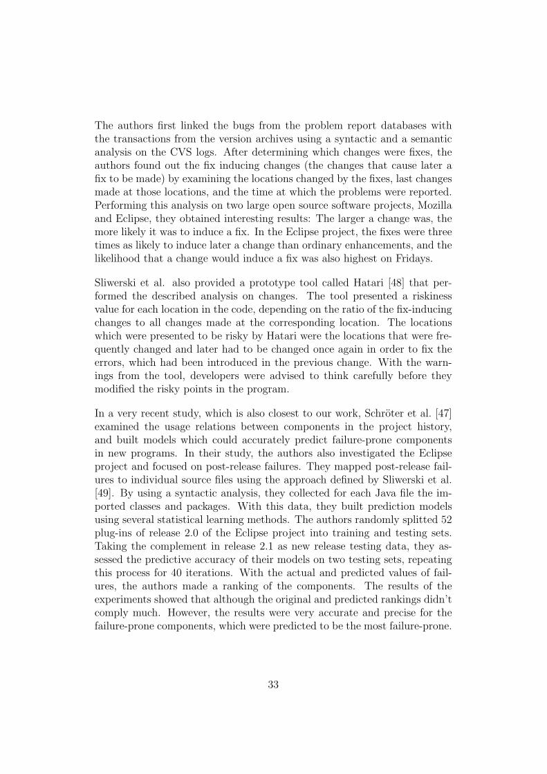
The authors first linked the bugs from the problem report databases withthe transactions from the version archives using a syntactic and a semanticanalysis on the CVS logs. After determining which changes were fixes, theauthors found out the fix inducing changes (the changes that cause later afix to be made) by examining the locations changed by the fixes, last changesmade at those locations, and the time at which the problems were reported.Performing this analysis on two large open source software projects, Mozillaand Eclipse, they obtained interesting results: The larger a change was, themore likely it was to induce a fix. In the Eclipse project, the fixes were threetimes as likely to induce later a change than ordinary enhancements, and thelikelihood that a change would induce a fix was also highest on Fridays.
Sliwerski et al. also provided a prototype tool called Hatari [48] that per-formed the described analysis on changes. The tool presented a riskinessvalue for each location in the code, depending on the ratio of the fix-inducingchanges to all changes made at the corresponding location. The locationswhich were presented to be risky by Hatari were the locations that were fre-quently changed and later had to be changed once again in order to fix theerrors, which had been introduced in the previous change. With the warn-ings from the tool, developers were advised to think carefully before theymodified the risky points in the program.
In a very recent study, which is also closest to our work, Schroter et al. [47]examined the usage relations between components in the project history,and built models which could accurately predict failure-prone componentsin new programs. In their study, the authors also investigated the Eclipseproject and focused on post-release failures. They mapped post-release fail-ures to individual source files using the approach defined by Sliwerski et al.[49]. By using a syntactic analysis, they collected for each Java file the im-ported classes and packages. With this data, they built prediction modelsusing several statistical learning methods. The authors randomly splitted 52plug-ins of release 2.0 of the Eclipse project into training and testing sets.Taking the complement in release 2.1 as new release testing data, they as-sessed the predictive accuracy of their models on two testing sets, repeatingthis process for 40 iterations. With the actual and predicted values of fail-ures, the authors made a ranking of the components. The results of theexperiments showed that although the original and predicted rankings didn’tcomply much. However, the results were very accurate and precise for thefailure-prone components, which were predicted to be the most failure-prone.
33

Input Cite Model Output
Product Metrics
[6] Spearman RankCorrelation
Failure Ranking
[5] Spearman RankCorrelation
Failure Ranking
[10] Several Statistical Failure CountMethods Failure-Proneness
Class
[16] CBR Faultiness Class
[17] Logistic Regression Failure-PronenessClass
[47] Several Statistical Failure CountMethods Failure-Proneness
Class
Product & ProcessMetrics
[30] CART Failure-PronenessClass
[31] ZIP Regression Fault Count
[32] SPRINT Faultiness Class
[34] CART Failure-PronenessClass
[38] Multiple Linear Failure DensityRegressionDiscriminant Failure-PronenessAnalysis Class
[40] Several RegressionModels
Failure Count
Pearson & SpearmanCorrelation
Failure Ranking
[41] Multiple LinearRegression
Failure Density
Product, Process &Execution Metrics
[33] Regression Tree Failure-PronenessClass
Product, Process,Usage & DeploymentMetrics
[36] Forward AICKendall & SpearmanRank Correlation
Failure CountFailure Ranking
Table 2.1: Summary of Related Studies without Historical Data
34

Input Cite Model Output
Product Metrics +Historical Data
[42] Multiple LinearRegression
Fault Count
[44] Negative BinomialRegression
Fault Count
[53] Negative BinomialRegression
Fault Count
Product, Process &Execution Metrics +Historical Data
[4] Regression ViaClassification
Faultiness Class
Product & ProcessMetrics +Historical Data
[23] Generalized LinearModels
Fault Count
[39] Pearson & SpearmanRank Correlation
Failure Ranking
Multiple LinearRegression
Failure Count
Historical Data [12] Logistic Regression Failure-PronenessClass
Table 2.2: Summary of Related Studies with Historical Data
35

Part A
Tokens and Risk Classes
36

Chapter 3
Initial Hypothesis
A software development project starts with an image of a system in themanagers’ and users’ minds. Later the requirements and specifications ofthe system are determined. In the design phase, the details of this system,its subsystems and components which will provide the required functionalityare determined. The following implementation stage brings all the ideas anddescriptions from earlier stages into life, and the source code of a projectis the realization of the system. The source code represents what has beendescribed with text, graphs and diagrams during the earlier phases by usinga pre-determined programming language.
The facilities provided by the programming languages used in the implemen-tation, and the complexity of the ideas that have to be realized determinehow easy or difficult it would be for the developers to bring the conceptsdefined in the design into life. These factors also affect the later stages wherethe correctness and the completeness of the implementation has to verified.The more mental burden a component puts on the developers, the harderit becomes to implement, test, and maintain it. The components which areharder to manage become later the problematic parts of the system.
When it comes to determining the complexity of a software system, theproject code may serve as a mirror that reflects the developers’ ability tounderstand and express what has been defined during the design phase. Fromthe project code, we can gather the valuable information which we can useto determine the parts of the project that are open to errors.
The source code of a project is composed of the code structures providedby the used programming languages. For example, the programs written in
37

today’s widely used object oriented languages are mainly composed of classdeclarations, which contain local or global variables, and method declara-tions. The classes are organized according to the inheritance relations al-lowed by the language, and unexpected behavior of the system is controlledwith the help of exception handling structures. In order to understand thecode, one has to examine these programming concepts and the correspondingstructures in the code.
Following these ideas, we defined our initial research hypothesis as follows:
H1 There is a relationship between code structures (i.e. calledmethod names, variable types, etc.) that exist in a soft-ware component and the failure-proneness of that component.Based on the appearance and the frequency of a set of specificcode structures in an entity, we can build models to predictits failure-proneness in the later releases.
In order to test this hypothesis, we inspected the source code of an open-source Java project, Eclipse. We called the code structures, in other wordsthe syntactic code pieces, such as ‘if’ statements, method names, or identifiersas tokens. After determining which tokens may be useful to give an overalldescription of the code, we examined the appearance of these tokens insidethe source files of the Eclipse project. Mining the problem tracking systemand version archives, we mapped the failures reported by the users to theindividual entities. Using the information about the failures and tokens, webuilt binary classification models that can predict whether a component isfailure-prone, based on the tokens in it. We used linear regression, logisticregression, and support vector machines methods to build our models, andwe evaluated the predictive accuracy of these models using precision andrecall values.
In this empirical case study, we wanted to answer the following questions:
1. Does this study provide evidence for or against our hypothesis?
• If yes, is there a specific type of tokens that helps the predictionof failures most? What kind of information about the programstructure does this token type provide?
2. How do different models compare to each other in accuracy? Whichmodel gives the most accurate predictions?
38

As we have seen in the previous chapter, various researchers have conductedstudies similar to ours. The contributions of our work are:
1. It introduces a new data source for predicting failure-prone compo-nents. Our predictions are focused on post-release failures, which aremore difficult and costly to fix than pre-release failures.
2. It presents predictive models that don’t need any specially computedmetrics data as input. Extracting token information and mapping fail-ures to software components is performed automatically. The need forhistorical data about failures is only limited to the training data set.
3. It provides a comparison of three frequently used statistical methods,based on their prediction accuracies.
4. Our models use data from different sets of token types as input, coveringdifferent aspects of object-oriented programming and their effects onfailures.
5. To our knowledge, it is the first study which examines the relationshipbetween various software tokens and post-release failures.
39

Chapter 4
Collecting Data
In this chapter, we give further information about the system under inspec-tion; how the failures in this system were found; how the failures could bemapped back to the individual components; the tokens which we looked for;and how we collected the information about these tokens.
4.1 Project under Inspection
The system that we inspected in this study is the Eclipse project [15]. Orig-inally developed by IBM, Eclipse is an open-source, platform-independentintegrated development environment (IDE) and application platform.
Eclipse is developed using the Java language, and its architecture is basedon plug-ins. Similar to an object in the object-oriented programming, aplug-in is an encapsulation of behavior and/or data that interacts with otherplug-ins to form a running program. Plug-ins may provide code, or onlydocumentation, resource bundles, or data to be used by other plug-ins.
Eclipse is composed of various projects. Eclipse Platform, Java Develope-ment Tools (JDT) and Plug-in Development Environment (PDE) subprojectstogether form the Eclipse Software Development Kit (SDK), which is also themain focus of our study. Although there are many projects in Eclipse, EclipseSDK is often called as the Eclipse project (In this study, we will also call theEclipse SDK project as the “Eclipse project”).
40
4.2 Determining Failure-Prone Entities
We gathered the data regarding the failure-prone entities in the Eclipseproject and the number of failures in these entities from the CVS versionarchive and the Bugzilla bug tracking system as follows:
1. The information about the entities (source files, classes, or methods)in the Eclipse project, and the changes made to these entities werecomputed by Zimmermann et al. [56]. In our study, we have reusedthis information.
2. In order to find out the post-release failures, we inspected the problemreports from the Bugzilla bug tracking system.
3. As we have seen in Section 2.2.3, Sliwerski et al. [49] computed themappings between the failures and the changes in the Eclipse project.Using these mappings, and the data from Step 1 and 2, we obtainedthe entities which were changed while fixing the post-release failures.
4. Finally, we classified those changed entities as failure-prone. The enti-ties which had been modified more were considered to be more failure-prone.
In the following sections, we will give further information about the stepsabove and the tools used in these steps.
4.2.1 CVS and Bugzilla
Concurrent Versions System (CVS) is an open source project, and a versioncontrol system which keeps track of all the work and changes in a set of files,typically the implementation of a software project. In addition to the changesmade to the files, CVS also keeps the answers to the following questions: whochanged which file, when, how and why. A change, also denoted as δ, mayinvolve insertions, deletions, or modifications of files. Each δ transformsa file from revision ri to revision ri+1. Several changes δ1, . . . , δn which areperformed by the same developer with the same intention (i.e. to fix a defect),committed at the same time, and containing the same log messages can beconsidered as the parts of a transaction, T . However, CVS doesn’t keep trackof transactions, and only records the changes made to files.
Similar to the transactions, the motive behind the changes is also not directlyrepresented in the CVS archives. In order to figure out whether a change was
41

made to fix a defect (as a result of a failure) or to add new functionality, onecan once again examine the log messages for the commits. Yet, in order tomake a better distinction between fixes and enhancements, and to determinewhen and in which versions of the Eclipse project the fixed failures werediscovered, further information from the Bugzilla bug tracking system isneeded.
Bugzilla [8] is a bug tracking system, originally developed and used by theMozilla Foundation. In addition to Mozilla and Eclipse, it is the bug trackingtool of choice for many other projects. It relies on a web server and a databasemanagement system which keeps the problem reports. The reports can besubmitted to Bugzilla by anybody, and they contain mainly the informationregarding the used version of the product, the operating environment, theproblem history and a brief summary of the problem. Some reports containthe enhancement requests, and such reports can be identified by looking atthe severity field of the reports, which is set to the value ‘ENHANCEMENT’in those cases. Inside the reports which are sent due to the failures, this fieldis set to some value between ‘CRITICAL’ and ‘TRIVIAL’.
In the lifecycle of a problem report, after the report is submitted, it is first val-idated, and the problem is checked not to be duplicate of an earlier reportedproblem. After the validation step, the problem is assigned to a developerwho examines and tries to solve it. The resolution for a problem report takesone of the following values: FIXED (The problem is fixed), INVALID (Theproblem is not a problem or doesn’t contain relevant facts), DUPLICATE(The problem already exists), WONTFIX (The problem will never be fixed),WORKSFORME (The problem couldn’t be reproduced).
4.2.2 Modified Entities
To find out the failure-prone components in the Eclipse project, it is necessaryto know which parts of the system were defective and fixed. Since severalparts of the system may be modified in the single fixes, the transactions inthe Eclipse project have to be found out, and in order to achieve this, ananalysis of the log messages, the committer, and the time of the commits inCVS is necessary.
Zimmermann et al. [56] conducted such an analysis, and computed the trans-actions from individual changes. The authors handled the time differences
42

Figure 4.1: Effects of Changes on Entities
between single commit operations using a sliding windows approach. In ad-dition to grouping the changes under the transactions, Zimmermann et al.also determined which parts of the Eclipse project were touched by thosechanges. In Figure 4.1, how changes may affect entities such as files, classes,or methods is demonstrated. To find the modified entities in Eclipse, for eachsource file, Zimmermann et al. compared each revision with its predecessor;determined the changed locations in the file; and mapped these locationsto the syntactic structures (classes and methods) in the files. In our study,to obtain the transactions and modified entities in the Eclipse project, wereused the results of Zimmermann et al.’s work [56].
4.2.3 Searching Problem Reports for Failures
In an earlier study [49], the problem reports for the Eclipse project weretransferred into a local database (of our research group) by Sliwerski et al.,using the XML export feature of the Bugzilla system. In our study, in orderto find the pre-/post-release failures, we examined the problem reports inthis database. We determined the reports that are related to the failures, bychecking whether
43

• the reports were reported “in the six months before/after the release”.
• the resolution field has the value “FIXED”.
• the severity field was set to some value other than “ENHANCEMENT”.
Taking into consideration that the new releases of the system are deliveredregularly, we decided to limit the post-release phase to a period which coveredthe first six months after the release. We believe that the users had sufficienttime in this period to install the system, use it, and discover most of thecommon problems. The time limitation on pre-release failures was madebecause of only the comparison reasons.
By checking the resolution field, the invalid and duplicate reports were elim-inated. The value “FIXED” indicated that the corresponding report wassent because of a failure, whose cause was later fixed. At this point, theseverity field helped us to differentiate the fixed failures from the fulfilledenhancement requests.
The numbers of pre- and post-release failures in several releases of the Eclipseproject are shown in Table 4.1. In our study, we examined two major releases,release 2.0 and release 2.1, for which we had enough post-release failure data.The minor releases weren’t considered due to the small number of failures.Among the remaining major releases, release 1.0 was also not included be-cause of the same reason. Since the system had gone under major changesbefore release 3.0, this release was also kept out of this study.
Version # Post-Release Failures # Pre-Release Failures
1.0 318 382.0 1662 69502.0.1 218 22.0.2 117 882.1 1222 41152.1.1 187 23.0 1762 57963.0.1 115 1
Table 4.1: Eclipse Project Failure History
44

4.2.4 Matching Changes and Failures
After gathering the information about all fine- and coarse-grained modifiedentities (source files, functions, classes) and the post-release failures in theEclipse project, in order to map the failures to these entities, we only neededthe links between the changes and failures in the Eclipse project. These linkswere computed by Sliwerski et al. [49].
In CVS archives, every change is annotated with a message that describesthe reason for that change. The numbers inside the messages usually cor-respond to a bug report number, so having a number inside the messagegives more confidence about a likely link between the change and the fail-ure. The keywords such as ‘fixed ’ or ‘bug ’ are also positive indicators of alink. Improving this approach of examining the messages in the CVS archivefor references to the bug reports, Sliwerski et al. [49] determined the linksbetween the transactions and failures in the Eclipse project. They assignedevery link (t, b) between a transaction t and a bug b two independent levels ofconfidence: a syntactic level, inferring links from a CVS log to a bug report,and a semantic level, validating a link via the bug report data. The authorsdetermined the links with significant syntactic and semantic confidence to bevalid. In our study, we used those links which were defined to be valid.
4.2.5 Defective/Failure-Prone Entities
After adding the information about the links between failures and transac-tions to our knowledge base, we had all the information that we needed tomap the failures to the entities. However, as one may argue, after joining thedata from these three sources, and finding the number of corrective changesmade to each entity, what we actually found was the number of defects inthose entities.
As we have mentioned in Section 2.1, for each post-release failure to occur,a post-release defect has to be introduced earlier. Even though a defectcan cause more than one failure, taking the number of post-release defectsas an estimate of the number of post-release failures is still a reasonableassumption. This approach of finding failure-prone entities was also appliedearlier by Nagappan et al. [40].
45

4.3 Token Information
For our predictive models, besides the number of failures in each entity,we have also used the information about the occurrences of tokens inside theentities. To understand the concept of tokens and how the information abouttheir occurrences can be collected, let’s first examine the code piece given inTable 4.2.
public class HelloWorld {public static void main(String[ ] args) {
System.out.println("Hello World!");
}}
Table 4.2: HelloWorld.java Source File
Like all other source files, HelloWorld.java file can also be decomposed intomeaningful code pieces such as modifiers (public), method names (main)and variable names (args). In our study, we called these significant pieces ofa program’s source code as tokens. In general, examples for tokens are con-stants (3.1425), identifiers (scanner), operators (==, <), keywords (while,if, break), and punctuations({, }, ;).
In order to extract the tokens from the source code, we used the AbstractSyntax Tree (AST) representation of the code. A possible AST for the ex-ample source file in Table 4.2, which is created using AST View Plugin [3]for Eclipse, is given in Table 4.3 and Table 4.4 together (For a better visual-ization, we have splitted the AST at the node where the subtree for the mainmethod’s body begins.). An abstract syntax tree is a structured representa-tion of the program text that captures the essential structure of the inputin a tree form. It omits unnecessary syntactic details such as punctuationswhich aren’t required in the tree structure.
As we can see from Table 4.3 and Table 4.4, even though the syntactic detailsare excluded, there are still several types of tokens inside an AST. Howevernot all of these tokens are necessary or helpful to understand the overallstructure of the program. Among various tokens, we selected the followingtoken types for the analysis of the Eclipse project:
1. AST Tokens: Tokens corresponding to the types of the nodes in theAST representation of the program, i.e. Modifier, SimpleName
46
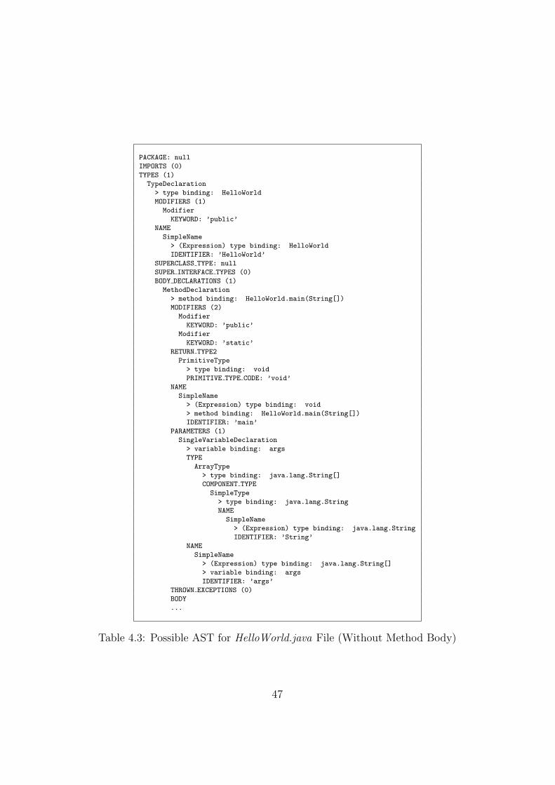
PACKAGE: null
IMPORTS (0)
TYPES (1)
TypeDeclaration
> type binding: HelloWorld
MODIFIERS (1)
Modifier
KEYWORD: ’public’
NAME
SimpleName
> (Expression) type binding: HelloWorld
IDENTIFIER: ’HelloWorld’
SUPERCLASS TYPE: null
SUPER INTERFACE TYPES (0)
BODY DECLARATIONS (1)
MethodDeclaration
> method binding: HelloWorld.main(String[])
MODIFIERS (2)
Modifier
KEYWORD: ’public’
Modifier
KEYWORD: ’static’
RETURN TYPE2
PrimitiveType
> type binding: void
PRIMITIVE TYPE CODE: ’void’
NAME
SimpleName
> (Expression) type binding: void
> method binding: HelloWorld.main(String[])
IDENTIFIER: ’main’
PARAMETERS (1)
SingleVariableDeclaration
> variable binding: args
TYPE
ArrayType
> type binding: java.lang.String[]
COMPONENT TYPE
SimpleType
> type binding: java.lang.String
NAME
SimpleName
> (Expression) type binding: java.lang.String
IDENTIFIER: ’String’
NAME
SimpleName
> (Expression) type binding: java.lang.String[]
> variable binding: args
IDENTIFIER: ’args’
THROWN EXCEPTIONS (0)
BODY
...
Table 4.3: Possible AST for HelloWorld.java File (Without Method Body)
47

...
BODY
Block
STATEMENTS (1)
ExpressionStatement
EXPRESSION
MethodInvocation
> (Expression) type binding: void
> method binding: PrintStream.println(String)
EXPRESSION
QualifiedName
> (Expression) type binding: java.io.PrintStream
> variable binding: System.out
QUALIFIER
SimpleName
> (Expression) type binding: java.lang.System
IDENTIFIER: ’System’
NAME
SimpleName
> (Expression) type binding: java.io.PrintStream
> variable binding: System.out
IDENTIFIER: ’out’
TYPE ARGUMENTS (0)
NAME
SimpleName
> (Expression) type binding: void
> method binding: PrintStream.println(String)
IDENTIFIER: ’println’
ARGUMENTS (1)
StringLiteral
> (Expression) type binding: java.lang.String
ESCAPED VALUE: ’"Hello World!"’
Table 4.4: Possible AST for HelloWorld.java File (Method Body)
2. Method Call Tokens: Names of the methods called in the program,i.e. main(...), getTime(...)
3. Variable Name Tokens: Names of the variables used in the program,i.e. args, candidateList, enum
4. Variable Type Tokens: Types of the variables used in the program,i.e. String, NumberFormat
5. Extends Tokens: Types of the classes that are inherited by otherclasses, i.e. Message, EnumerationFilter
6. Implements Tokens: Types of the interfaces that are implementedby other classes, i.e. Cloneable, IResponse
7. Throws Tokens: Types of the exceptions that may be thrown bya function, also specified in function declarations using throws state-ment, i.e. IllegalArgumentException
48

8. Throw Tokens: Types of the exceptions that are thrown inside thefunction using throw statement, i.e. IOException
9. Catch Tokens: Types of the exceptions that are caught inside thetry-catch blocks, i.e. NoSuchElementException
To create the AST representations of the source files in the Eclipse project,and to search for the tokens in these representations, we used the Eclipseproject itself. JDT subproject provided us with the necessary classes, firstto create (ASTParser), and later to examine the AST (ASTVisitor) for agiven source file. To determine the tokens of interest, we examined thetype attribute of the ASTNode class, which tells to which code structure(MethodDeclaration, SimpleType, etc.) a node corresponds. Re-implement-ing the methods of the ASTVisitor class, we handled distinct AST nodes andextracted our tokens.
We have performed token extraction at three different granularity levels(source file, class, and method levels) and collected the token informationin a local database. Table 4.5 shows the tokens collected from the code snip-pet given in Table 4.2 at source file level. In addition to the name of thefile from which the tokens were extracted (which has been omitted in Ta-ble 4.5 due to space limitations), each record in our token database kept theinformation about:
• the name of the entity in which the token was located
• the type of the token
• the name of the token instance, which is
– for AST tokens, the type attribute of the corresponding node
– for method call tokens, the method name
– for variable name tokens, the variable name
– for other tokens, the type of class, interface, or exception, depend-ing on the token type
• for method call tokens, the number of arguments in the called method
• the number of occurrences of the token instance
49

Entity Name Token Type Instance Name Arg.s Count
HelloWorld.java AST Expression Statement 1HelloWorld.java AST Method Declaration 1HelloWorld.java AST Method Invocation 1HelloWorld.java AST Primitive Type 1HelloWorld.java AST Qualified Name 1HelloWorld.java AST Simple Name 7HelloWorld.java AST Simple Type 1HelloWorld.java AST Single Variable Declaration 1HelloWorld.java AST String Literal 1HelloWorld.java AST Array Type 1HelloWorld.java AST Type Declaration 1HelloWorld.java AST Block 1HelloWorld.java AST Modifier 3HelloWorld.java Method Call println * 1HelloWorld.java Variable Type String[ ] 1HelloWorld.java Variable Name args 1
Table 4.5: Tokens for HelloWorld.java at Source File Level
50

Chapter 5
Preliminaries
In our study, we used linear regression, logistic regression and support vectormachine methods to build predictive models. We assessed the accuracy ofour models with the help of precision and recall measures.
5.1 Statistical Methods
We utilized statistical methods to discover how one or more predictor vari-ables (features, attributes, independent variables) affected the response vari-able (dependent variable). Such an analysis is called regression.
5.1.1 Linear Regression
Linear regression is called ”linear” because the relation of the dependentvariable to the independent variables is assumed to be a linear function ofsome parameters. The simplest version of linear regression is:
y = b + wx + ε
where there is a single independent variable, x. In general, the models of theform
y = b + w1x1 + w2x2 + . . . + wkxk + ε
51

with k > 1 independent variables are called multiple linear regression models.The w’s and b are called the parameters, and the ε is the error. The b isthe constant where the regression line intercepts the y-axis, representing thevalue that y takes when all the independent variables are ‘0’. The w’s are theweights for the independent variables, and they represent the amount thatthe dependent variable y changes when the corresponding attribute changesby ‘1’ unit. Although the values for the parameters aren’t known, they canbe estimated using the observations at hand.
With the instances x = (x1, . . . ,xk) coming from n observations, we canpredict the output y via the following model:
yi = b +k∑
j=1
wjxij + εj where i = 1, 2, . . . , n
This model can also be written in the matrix representation where the pa-rameter b can be included in the parameters list W by adding a constantattribute to the attributes list.
Y =
y1
y2
...yn
,X =
1 x11 . . . x1k
1 x21 . . . x2k
1...
. . ....
1 xn1 . . . xnk
,W =
bw1...
wk
, ~ε =
ε1
ε2...εn
Y = XW + ~ε
In this model, the smaller the residuals ε (the differences between the actualobservations yi and the predicted values yi), the better is the fit. The mostpopular method of finding the estimates for the parameters wj and b, whichgive the best fit, is the method of least squares. In this method, the valuesfor the coefficients which minimize the sum of the squared residuals is found.Figure 5.1 from Hastie et al. [26] illustrates the least squares fitting in R2.
The least-square estimators wj and b aren’t only easy to compute but, underthe Gauss-Markov assumptions, also the best estimators for the unknownparameters. According to Gauss-Markov assumptions:
1. E(εi) = 0 (Expected value of errors is 0).
2. εi’s are independent.
3. εi’s are normally distributed.
4. ∀i V ar(εi) = σ2 (Errors all have the same variance).
52
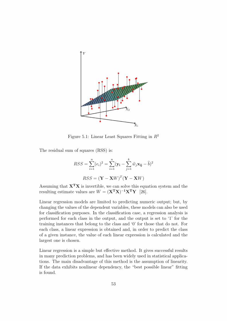
Figure 5.1: Linear Least Squares Fitting in R2
The residual sum of squares (RSS) is:
RSS =n∑
i=1
(ei)2 =
n∑
i=1
(yi −k∑
j=1
wjxij − b)2
RSS = (Y − XW )T (Y − XW )
Assuming that XTX is invertible, we can solve this equation system and theresulting estimate values are W = (XTX)−1XTY [26].
Linear regression models are limited to predicting numeric output; but, bychanging the values of the dependent variables, these models can also be usedfor classification purposes. In the classification case, a regression analysis isperformed for each class in the output, and the output is set to ‘1’ for thetraining instances that belong to the class and ‘0’ for those that do not. Foreach class, a linear expression is obtained and, in order to predict the classof a given instance, the value of each linear expression is calculated and thelargest one is chosen.
Linear regression is a simple but effective method. It gives successful resultsin many prediction problems, and has been widely used in statistical applica-tions. The main disadvantage of this method is the assumption of linearity.If the data exhibits nonlinear dependency, the “best possible linear” fittingis found.
53

5.1.2 Logistic Regression
Although we can use linear regression to predict the classes for the instances,the returned values aren’t always within [0, 1] interval, so they aren’t properprobabilities. Logistic regression estimates the “odds” of an instance belong-ing to a class, rather than approximating the ‘0’ and ‘1’ values directly. Itreplaces the original target variable in linear regression Pr[1|x1, x2, . . . , xk]with
logPr[1|x1, x2, . . . , xk]
1 − Pr[1|x1, x2, . . . , xk]
where the resulting values are between −∞ and ∞. This transformation iscalled the logit transformation, and the name “logit” comes from the logitfunction logit(p) = log(p/1 − p), which is shown in Figure 5.2.
The transformed variable is approximated once again using a linear function,as it is in linear regression. The resulting model is now given as:
Pr[1|x1, x2, . . . , xk] =exp(b + w1x1 + w2x2 + . . . + wkxk)
1 + exp(b + w1x1 + w2x2 + . . . + wkxk)(∗)
As in the case of linear regression, the estimates for the parameters w’s and bthat fit the training data best are sought. However, unlike linear regression,which uses the least squares method, logistic regression uses the maximumlikelihood method to find the estimates. The method tries to maximize thevalue of the log-likelihood function.
The likelihood of a set of data is the probability of obtaining that this par-ticular set, given the chosen probability distribution model. Log-likelihoodfunction is simply the logarithm of the likelihood function. For the binary
Figure 5.2: Logit Function
54
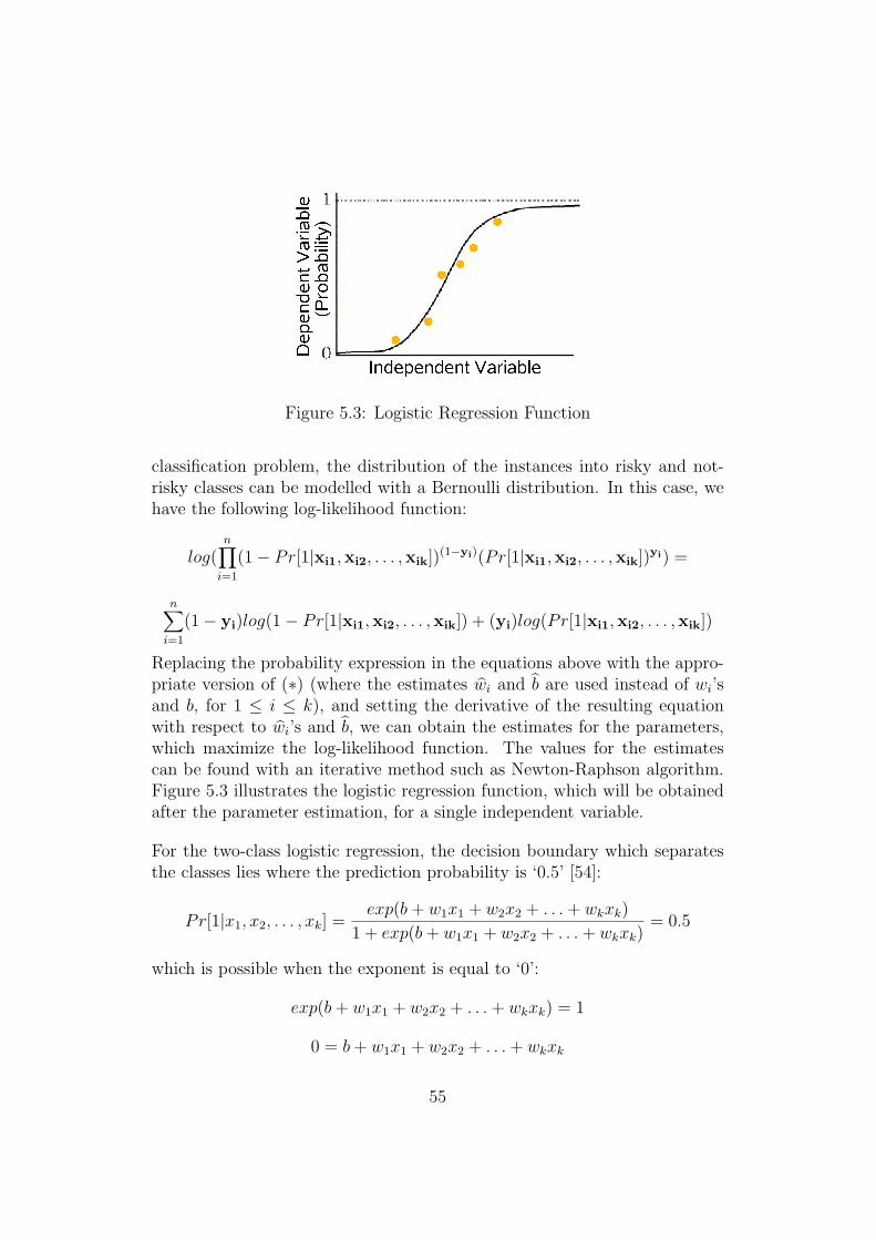
Figure 5.3: Logistic Regression Function
classification problem, the distribution of the instances into risky and not-risky classes can be modelled with a Bernoulli distribution. In this case, wehave the following log-likelihood function:
log(n∏
i=1
(1 − Pr[1|xi1,xi2, . . . ,xik])(1−yi)(Pr[1|xi1,xi2, . . . ,xik])
yi) =
n∑
i=1
(1 − yi)log(1 − Pr[1|xi1,xi2, . . . ,xik]) + (yi)log(Pr[1|xi1,xi2, . . . ,xik])
Replacing the probability expression in the equations above with the appro-priate version of (∗) (where the estimates wi and b are used instead of wi’sand b, for 1 ≤ i ≤ k), and setting the derivative of the resulting equationwith respect to wi’s and b, we can obtain the estimates for the parameters,which maximize the log-likelihood function. The values for the estimatescan be found with an iterative method such as Newton-Raphson algorithm.Figure 5.3 illustrates the logistic regression function, which will be obtainedafter the parameter estimation, for a single independent variable.
For the two-class logistic regression, the decision boundary which separatesthe classes lies where the prediction probability is ‘0.5’ [54]:
Pr[1|x1, x2, . . . , xk] =exp(b + w1x1 + w2x2 + . . . + wkxk)
1 + exp(b + w1x1 + w2x2 + . . . + wkxk)= 0.5
which is possible when the exponent is equal to ‘0’:
exp(b + w1x1 + w2x2 + . . . + wkxk) = 1
0 = b + w1x1 + w2x2 + . . . + wkxk
55

Since this is a linear equality, the boundary is a linear hyperplane. So logis-tic regression also suffers from the same problem as linear regression does,namely the non-linearly separable data. Yet, logistic regression has the de-scribed advantages over linear regression with binary dependent variables.
5.1.3 Support Vector Machines
In the classification models, the instances, each of which can be representedwith an attribute vector of k numbers, may also be regarded as points in ank-dimensional instance space. If the classes are linearly separable, there is ahyperplane in this space that classifies all instances correctly.
For a given set of points, there may be many hyperplanes that achieve aclear separation of the classes, as we can see in Figure 5.4. Among thesehyperplanes, the hyperplane that is as far away as possible from the pointsin both classes is called the maximum margin hyperplane. The points that areclosest to the maximum margin hyperplane are called the support vectors [11].The maximum margin hyperplane and the corresponding support vectors forthe data set from Figure 5.4 can be seen in Figure 5.5.
In the process of finding the maximum margin hyperplane, assuming thatthe classes of the instances are represented with values of +1 and -1, wetry to determine w ∈ Rk such that δ, the distance of the maximum marginhyperplane to each class, is maximized subject to
yi
1
‖w‖(w · xi + b) ≥ δ, i = 1, . . . , n
Figure 5.4: Separating Hyperplanes Figure 5.5: Support Vectors andMaximum Margin Hyperplane
56

As stated in [9], this problem is equal to finding α1, . . . , αn ∈ R+0 such that
n∑
i=1
αi −1
2
n∑
i=1
n∑
j=1
yiyjαiαj(xi · xj) is maximized,n∑
i=1
yiαi = 0 and ∀αi ≥ 0
Solving this system, which is a special mathematical optimization problemcalled “quadratic programming”, gives the optimal values for the parameters:
wk =n∑
i=1
αiyixik where αi > 0 only for support vectors
b = yi − w · xi for any support vector xi
Here it is important that, given the support vectors, one can construct themaximum margin hyperplane. The other instances are irrelevant for thedecision boundary. The hyperplane can be defined as:
y = b +∑
xi∈S
αi yi (xi · x)
where S is the set of support vectors. Following this property, support vectormachines (SVM) method takes its name from the support vectors.
As we have mentioned in the earlier prediction methods, some real-worldproblems involve data which can’t be clearly separated by any linear bound-ary. In order to learn the non-linear relations using a linear method, one canselect a set of non-linear features, and rewrite the data in this new represen-tation. Then, the linear model in the new feature space will be:
y = b +N∑
i=1
wiφi(x)
where φ : X → F is a non-linear mapping from the input space to the featurespace, which has N attributes.
As we can see from Figure 5.6, the non-linear models are built in two steps:first by transforming the data into a feature space F by a fixed non-linearmapping, φ, and then by classifying them in the feature space using a linearmodel.
In the maximum margin hyperplane equation, we have seen that we have toperform a dot product between the new instance x and all support vectorsxi in order to classify x. In the high dimensional feature space, a similarsituation exists:
y = b +∑
xi∈S
αi yi 〈φ(xi), φ(x)〉
57

With the increasing number of attributes in the feature space, the transfor-mation and following dot product can be very costly. On the other hand,computing the dot product 〈φ(xi), φ(x)〉 in the feature space directly as afunction of the original inputs makes it possible to join the two steps to buildour non-linear model. Such a direct computation method is called a kernelfunction.
A kernel is a function K, such that
K(~x, ~z) = 〈φ(~x), φ(~z)〉 for all ~x, ~z ∈ X
where φ is a mapping from X to a feature space F . An important consequenceof this representation is that we don’t have to consider the dimension of thefeature space in our computations. Some common kernel functions are:
• Polynomial : K(x, x′) = (x · x′)d
• Radial Basis Function: K(x, x′) = exp(−γ‖x − x′‖2), for γ > 0
• Sigmoid: K(x, x′) = tanh(κx · x′ + c), for some κ > 0 and c < 0
The so-called “kernel trick” makes it possible to map the data into the fea-ture space implicitly and train a linear model in this space, overcoming thecomputational problems. The hyperplane in the feature space may be non-linear in the instance space, allowing SVM method to handle non-linearlyseparable data points as well.
In the SVM models, a general problem with other linear models, namelythe overfitting, is also less likely to occur. Whereas changing some instanceswould make significant changes in the decision boundary in the other models,the maximum margin hyperplane would only change if training instances thatare the support vectors are added or deleted.
Figure 5.6: Transformation from Instance Space to Feature Space
58

If the training data can’t be separated linearly or non-linearly without error,SVM use the “soft margin” method [11] to choose a hyperplane that splitsthe instances as neatly as possible, while still maximizing the distance to thenearest cleanly split examples. The error term ξ is introduced for the in-stances which are positioned on the wrong side of the separating hyperplane.
w · xi + b ≥ +1 − ξi for yi = +1
w · xi + b ≤ −1 + ξi for yi = −1
∀ξi ≥ 0
The cost of errors is introduced into the optimization problem as a summa-tion,
∑ni=1 ξi weighted with a parameter C, which has to be minimized while
the margin is kept at maximum. Giving a larger value to the parameter Ccorresponds to assigning a higher penalty to the errors. With this additionalconstraint, the initial problem of finding w and b stays the same. Yet the αvalues have an upper bound: 0 ≤ αi ≤ C.
In addition to class values, SVM could also be used for predicting numeri-cal values. The idea is similar to linear regression, finding a function thatapproximates the training points well by minimizing the prediction error.Different from linear regression, in support vector regression, the regressionfunction depends on a subset of the training data. The training points thatlie beyond a user-specified margin aren’t included in the cost function forbuilding the model [54]. Overfitting is reduced by trying to maximize theflatness of the regression function while the error is minimized. This problemcould also be solved with an approach similar to the soft margin method.
59

Linear Regression
⊖ Best results are obtained whenrelations between independentand dependent variables arelinear
⊕ It has a well-understood the-ory behind, and has beenwidely used
⊖ It is sensitive to outliers (un-usual data points in trainingdata)
⊕ Weights indicate relative im-portance of each feature
⊖ Decision boundary is linearand can handle only linearlyseparable data
⊕ It can be used for both binaryclassification, and regression
⊕ It is simple and easy to use
Logistic Regression
⊖ Predictions limited to [0, 1]range, therefore no failurecount prediction is possible
⊕ Predictions are proper proba-bilities (they don’t exceed 0-1interval)
⊖ Resulting models are more dif-ficult to interpret
⊕ It requires fewer statistical as-sumptions than linear regres-sion
⊖ Like linear regression, decisionboundary is linear
Support Vector Machines
⊖ Computational complexity ishigher (number of support vec-tors may increase for largerdata sets)
⊕ Soft-margin method handlescases for which classificationscan be made only with errors
⊖ Models are less intuitive andmore difficult to interpret
⊕ It can be used for classificationand regression purposes
⊖ Selection of kernel function pa-rameters is an open problem
⊕ Kernel trick enables non-linearboundaries
⊕ It is affected less by outliers
Table 5.1: Summary of Statistical Methods
60
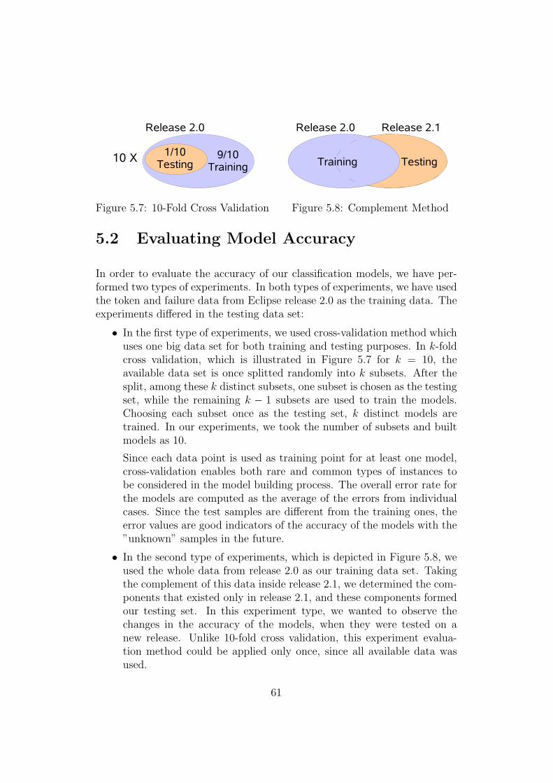
Figure 5.7: 10-Fold Cross Validation Figure 5.8: Complement Method
5.2 Evaluating Model Accuracy
In order to evaluate the accuracy of our classification models, we have per-formed two types of experiments. In both types of experiments, we have usedthe token and failure data from Eclipse release 2.0 as the training data. Theexperiments differed in the testing data set:
• In the first type of experiments, we used cross-validation method whichuses one big data set for both training and testing purposes. In k-foldcross validation, which is illustrated in Figure 5.7 for k = 10, theavailable data set is once splitted randomly into k subsets. After thesplit, among these k distinct subsets, one subset is chosen as the testingset, while the remaining k − 1 subsets are used to train the models.Choosing each subset once as the testing set, k distinct models aretrained. In our experiments, we took the number of subsets and builtmodels as 10.
Since each data point is used as training point for at least one model,cross-validation enables both rare and common types of instances tobe considered in the model building process. The overall error rate forthe models are computed as the average of the errors from individualcases. Since the test samples are different from the training ones, theerror values are good indicators of the accuracy of the models with the”unknown” samples in the future.
• In the second type of experiments, which is depicted in Figure 5.8, weused the whole data from release 2.0 as our training data set. Takingthe complement of this data inside release 2.1, we determined the com-ponents that existed only in release 2.1, and these components formedour testing set. In this experiment type, we wanted to observe thechanges in the accuracy of the models, when they were tested on anew release. Unlike 10-fold cross validation, this experiment evalua-tion method could be applied only once, since all available data wasused.
61

Predicted Risky Predicted Risky
True Risky r11 r12
True Not-Risky r21 r22
Table 5.2: Correspondence of Real and Predicted Results
In both experiment types, before starting a experiment, we determined arisk class for each testing instance: risky (failure-prone) if failure count wasgreater than ‘0’, or not-risky (not failure-prone) if failure count was equal to‘0’. Once the predictions were made by the statistical models, we had over-lapping sets of original and predicted risk classes, which can be representedas in Table 5.2.
Assuming that developers and managers would like to know which compo-nents are failure-prone, and how many such components there are in theirprojects, we set our main goal as finding the risky components, and set ourevaluation measures accordingly. From the fields of Table 5.2, we computedtwo measures, precision and recall, which are also used in Information Re-trieval studies in order to evaluate the search strategies. In our study, wehave modified these measures according to our needs:
Precision is the ratio1 of the number of components which are risky andclassified as risky, to the total number of components which are classi-fied as risky.
Precision =r11
r11 + r21
Recall is the ratio1 of the number of components that are risky and alsoclassified by the predictor as risky, to the total number of componentswhich are risky.
Recall =r11
r11 + r12
The precision values showed the purity of our results, namely how much ofthe components that were classified as risky were indeed risky in reality. Soit was an indicator of how credible our models were when they marked acomponent to be risky. On the other hand, the recall values showed howmuch of the risky components our prediction models covered, so how wellthe managers and developers would be informed about the number of realrisky components.
1Although precision and recall are defined as ratios, in some cases, we have regardedthese measures as percentages as well
62

Chapter 6
Classification Models andResults
In this chapter, we will first explain some details of our classification models,and later examine the results of these models. Finally, we will compare themodels with each other based on these results.
6.1 R System
The system in which we built our prediction models is the R system [46].The R system consists of a programming language, and a run-time environ-ment which provides graphics support, access to some system functions anda debugger. The system also has the ability to run programs stored in scriptfiles. The R distribution contains functionality for a large number of statis-tical procedures such as linear and nonlinear regression models, clustering,and smoothing. There is also a large set of functions which enables the cre-ation of various kinds of data presentations. Further information about theR system can be obtained from R FAQ page [27].
6.2 Input Format
As the input to the R system, we have given the token and failure informa-tion from the training set in a plain data file. An example input file had
63

Figure 6.1: Classification Experiments Input Format
the matrix structure shown in Figure 6.1. Each row in such an input matrixcontained the information about a single instance (component). The firstcolumn showed the failure-proneness class of the instances, taking the value‘1’ for failure-prone components. The features which corresponded to thetoken types inside the training components were represented in the columns,starting from the second one. The values in these columns showed, for thecorresponding component, how many times the different tokens, i.e. a vari-able with name foo or an exception of type IOException, appeared in thatcomponent.
Like the training data, the testing input also followed the pattern in Fig-ure 6.1. However in the testing case, the first column wasn’t involved in theprediction process, and was used only for the comparison of the actual andpredicted values.
6.3 Joining Failure and Token Information
To obtain the input matrices, the failure and token information stored intwo separate databases had to be joined. As illustrated in Figure 6.2, thenames of the files were used for this purpose, since this field was common inboth databases. In some cases where the source files had been relocated, orthe directory structure had been modified before the release, we had somedifferences in the file names, which also lead to the problems in matching.To overcome these problems, we performed a two-phase matching betweenthe file names:
• Initially, we handled the files whose names matched exactly, and weexcluded those files from further processing.
64

Figure 6.2: Joining Failure and Token Databases
• For the remaining files, we have performed a prefix, suffix and deepsuffix comparison between the file names.
– First, we have compared the names of the plug-ins to which thefiles belonged. If the plug-in names (prefixes) matched, then wechecked whether the source file names and the name of the lastdirectory in the path (suffixes) were the same.
– When the plug-in names didn’t correspond, we compared the filenames and the names of the last two directories in the path (deepsuffixes).
In this process, every file from the token database was mapped to the first filefrom the failure database, for which there was a suffix or deep-suffix match.Our inspections on the results showed that our suffix and deep suffix checksgave in almost all cases correct matchings, supporting the validity of ourmethod. Here are some example matchings:
• Example (a)
org.eclipse.ant.core/org/eclipse/ant/core/AntCorePlugin.java↓ matches
org.eclipse.ant.core/src/org/eclipse/ant/core/AntCorePlugin.java
65
• Example (b)
org.eclipse.compare/org/eclipse/compare/CompareUI.java↓ matches
org.eclipse.compare/compare/org/eclipse/compare/CompareUI.java
• Example (c)
org.eclipse.ui/org/eclipse/jface/text/TextViewer.java↓ matches
org.eclipse.jface.text/src/org/eclipse/jface/text/TextViewer.java
6.4 Token Groups
In Section 4.3, we have explained the types of tokens that we extractedfrom the code. While creating our input files, we grouped these token typesin subsets which covered different programming aspects. Although it waspossible to come up with other combinations of tokens, we believe that thesubsets below covered the most important programming concepts from theobject-oriented programs.
AST Tokens: (Abstract Syntax Tree Tokens) AST tokens provide a sum-mary of the overall program structure, and they also hold the informa-tion about some of the metrics used in the earlier studies such as thenumber of method calls, variables in a component.
Inheritance Tokens: (Extends and Implements Tokens) Inheritance to-kens show the inheritance relations between classes and interfaces.With these tokens, it may possible to determine whether risk prop-agates from the super-classes/interfaces to the sub-classes/interfaces.
Method Call Tokens: (Method Call Tokens) The number of methods acomponent calls, or the number of methods called from a specific com-ponent have been used as product metrics in the earlier studies. Similarto those metrics, the method call tokens give us the information aboutwhich component called which function and how many times the com-ponent called this function.
Exception Tokens: (Throws, Throw and Catch Tokens) Exception tokensprovide an insight to the exceptions, the exceptional events that dis-rupt the normal flow of the program’s instructions. Exceptions thrownduring program run or methods which might throw an exception areimportant points in the program where extra attention should be paid.
66

Variable Tokens: (Variable Type and Name Tokens) The variables used ina component show on which other classes the functionality of a com-ponent depends. Based on used variables and their types, it might bepossible to make inductions about complex and problematic structures,or problem domains.
The total number of distinct instances in these token groups, which alsodefined the number of columns in our data matrices, are shown in the thirdcolumn of Table 6.1. As we can see from this table, we had large numbersof features for method call and variable tokens. Considering that we had6751 files in release 2.0, and a row was created for each component (at thebroadest granularity, for each file), it’s not difficult to see how large our datamatrices for some token types were. (i.e. at file level, for method call tokens,the data matrix had more than 177 million cells).
The problems with the big data matrices were the time that it took to trainthe models and the memory requirements (the computer we have used inour initial experiments had a single 2.4 GHz processor and 1 GB of mainmemory). The model building times became a bigger problem especially inthe experiments with the cross-validation technique where the model had tobe trained 10 times, every time with almost the whole data set ( 9
10of release
2.0 data). Since the R system needs to keep the whole data in the mainmemory, we weren’t able to perform some experiments with very large datasets.
In order to improve the run-time of our experiments and to overcome memorylimitations, we restricted all of our experiments in terms of the instance
Token Name # Instances Total Total (Restricted)
AST 61 61 —
Implements 9182113 —
Extends 1195
Method Call 26289 26289 2628
Catch 130326 —Throw 115
Throws 81
Var. Type 504944374 2219
Var. Name 39325
Table 6.1: Number of Instances in Token Groups under Examination
67

granularity, and some experiments also in terms of the inspected tokens. Asfor granularity, we conducted the experiments only at file level where wehad the least number of instances. (For release 2.0, we had 6751 files, 7701classes, and 74838 distinct methods)
To decrease the number of columns for method call and variable tokens, forwhich we had the highest number of features in Table 6.1, we have per-formed a frequency analysis and determined which token types existed mostfrequently in the files. After sorting the tokens based on frequency, we havetaken top-10% of method call and top-5% of variable tokens. The corre-sponding features counts are shown in the third column of Table 6.1. Thesetop-10% and top-5% of token types covered more than 75% of the totaloccurences of tokens of those types, and the results of our experiments ofsmaller scales indicated that such a limitation of features didn’t affect theresults significantly.
6.5 Random Classifier
In Section 5.2, we stated that the precision and recall measures were used toevaluate our models. Based on these values, we have compared our classifica-tion models not only against each other, but also against a random classifier.With the random guessing strategy, we considered the case in which we hadno information available to help us during the classification process.
In the random classification model, each instance is put into one of the riskclasses with an equal likelihood of 0.5. With such a classification strategy,since the risky instances would be correctly classified for half of the cases,we took the recall value as ‘0.5’. Since the classification with the randomclassifier, and the classification in real life are independent events; the pre-cision values for the random models were determined to be the ratio of thefailure-prone files in the release 2.0, and release 2.1 testing data. The follow-ing equations demonstrate how the precision and recall values are computedfor the random classifier:
If P(Risky) = p, then
Precision =P(Risky ∧ Pred. Risky)
P(Pred. Risky)=
P(Risky) · P(Pred. Risky)
P(Pred. Risky)=
p ∗ 0.5
0.5= p
Recall =P(Risky ∧ Pred. Risky)
P(Risky)=
P(Risky) · P(Pred. Risky)
P(Risky)=
p ∗ 0.5
p= 0.5
68

6.6 Building Classification Models
In this study, we used our R-scripts to build linear regression, logistic re-gression and support vector machines models. The statistical model buildingfunctions had already been provided in the R system (lm and glm in the de-fault distribution, and svm in the ‘e1071’ library for the R system [14]) andwe have used the default parameters of the methods. The support vectormachines models were built for classification purposes (type parameter ofsvm method determines the model type), and we have used the radial basisfunction as kernel, as it was recommended by Hsu et al. [28], and also byMeyer [37] for the initial experiments with the SVM models.
The risk classes for the testing instances were computed using the thresh-olding technique on the predicted riskiness values, with the threshold valueof ‘0.5’. Although we chose this value since it was the middle point betweenthe values for the risk classes, it was also possible to determine the thresholdusing ROC curves, as it had been done by El-Emam et al. [17].
6.7 Results from Classification Models
In this section, we present the results of our experiments. The results fromthe cross-validation and complement method experiments are shown sepa-rately. In each experiment group, the results are given in a precision-recallgraph where the x-axis corresponds to the recall values and the y-axis holdsthe precision values. For the cross-validation experiments, the precision andrecall values are the averages of the ten precision and recall values com-puted for the ten testing subsets. The precision and recall values for theexperiments with the complement method were computed once on release2.1 testing data.
In the precision-recall graphs, we have marked some of the results, which werethe maximal points. A planar point (x1, y1) dominates (x2, y2), if x1 > x2
and y1 > y2; and a point (x, y) is called a maximal point, if no other pointdominates it. Maximal points are of interest as they show either higher recallor precision values than the other points.
69
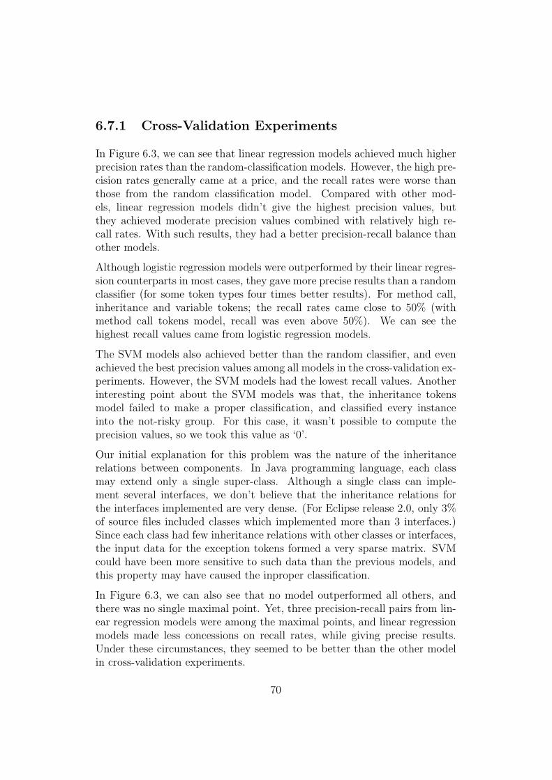
6.7.1 Cross-Validation Experiments
In Figure 6.3, we can see that linear regression models achieved much higherprecision rates than the random-classification models. However, the high pre-cision rates generally came at a price, and the recall rates were worse thanthose from the random classification model. Compared with other mod-els, linear regression models didn’t give the highest precision values, butthey achieved moderate precision values combined with relatively high re-call rates. With such results, they had a better precision-recall balance thanother models.
Although logistic regression models were outperformed by their linear regres-sion counterparts in most cases, they gave more precise results than a randomclassifier (for some token types four times better results). For method call,inheritance and variable tokens; the recall rates came close to 50% (withmethod call tokens model, recall was even above 50%). We can see thehighest recall values came from logistic regression models.
The SVM models also achieved better than the random classifier, and evenachieved the best precision values among all models in the cross-validation ex-periments. However, the SVM models had the lowest recall values. Anotherinteresting point about the SVM models was that, the inheritance tokensmodel failed to make a proper classification, and classified every instanceinto the not-risky group. For this case, it wasn’t possible to compute theprecision values, so we took this value as ‘0’.
Our initial explanation for this problem was the nature of the inheritancerelations between components. In Java programming language, each classmay extend only a single super-class. Although a single class can imple-ment several interfaces, we don’t believe that the inheritance relations forthe interfaces implemented are very dense. (For Eclipse release 2.0, only 3%of source files included classes which implemented more than 3 interfaces.)Since each class had few inheritance relations with other classes or interfaces,the input data for the exception tokens formed a very sparse matrix. SVMcould have been more sensitive to such data than the previous models, andthis property may have caused the inproper classification.
In Figure 6.3, we can also see that no model outperformed all others, andthere was no single maximal point. Yet, three precision-recall pairs from lin-ear regression models were among the maximal points, and linear regressionmodels made less concessions on recall rates, while giving precise results.Under these circumstances, they seemed to be better than the other modelin cross-validation experiments.
70

Figure 6.3: Precision-Recall Values from Cross-Validation Experiments
Figure 6.4: Precision-Recall Values from Complement Experiments
71

6.7.2 Complement Method Experiments
Figure 6.4 shows the results from the complement method experiments. Inthis figure, we can notice that the precision values for all models lie below‘0.4’, which indicates a clear decrease in precision. We believe that the re-striction on the attributes of testing data might have been a reason for thisdecrease.
In our models, the testing data was classified based on the occurrences of thetokens which were used in training. This meant that the tokens which existedonly in release 2.1 weren’t taken into consideration. In the data matrix, thisrestriction may have resulted in rows which contained fewer columns withpositive values, and the unhealthy predictions may have been caused as aresult of the insufficient data.
Even under these circumstances, the linear regression models (except themodel for AST tokens) performed once again better than the random clas-sifier in terms of the precision values. The ‘exceptionally high’ recall valuecoming from the model with AST tokens took our interest, and our inspec-tions on the distribution of classified instances showed that the linear regres-sion model achieved this result by classifying almost every instance as risky.We believe that the limitation on token types or some outlier values mighthave caused this erroneous classification.
Logistic regression models had better precision values than the random clas-sifier. Their recall values were similar to those from the linear regressionmodels, but they achieved lower precision values than linear regression mod-els. With these values, linear regression was once again superior to logisticregression.
For SVM models, the misclassification problems continued also with the testdata from release 2.1. For three models (AST, variable & method call), theSVM models put every instance into the not-risky class, making a precisioncalculation impossible. We have taken the precision rates for those cases as0, as in the case with the cross validation experiments. For the other modelswhich provided non-zero precision rates, our examinations showed that onlya few risky files were correctly classified as risky, and a few (but more) not-risky files were also classified to be risky. As a result, the precision rateswere deceptively better than those from the random classification model.However, if we would think in terms of the number of correctly classifiedfiles, the random classifier was actually better. So, SVM seemed to performworse than the other models on release 2.1 testing data.
72

We believe that, in addition to the limitations on the attributes, the parame-ters selected for the kernel functions may have also caused the problems withthe SVM models. As we have mentioned earlier, the parameter selectionprocess itself is an open problem, and as it was suggested by Hsu et al. [28],a “grid search” may be applied to find better parameters. Yet, in this study,due to the large size of inputs and time limitations, we couldn’t perform athrough search for the optimal parameters.
In the experiments with the complement method, the linear regression modelsonce again seemed to have achieved better than the other models. However,as it was in the earlier case, we didn’t have a single maximal point.
6.8 Conclusion
The results from the classification experiments at the file level showed thatour models performed in most experiments better than a random classifica-tion model in terms of precision. In some cases, our models even achievedbetter recall values than the random model.
We think that, while evaluating the models, the high recall values can besacrificed in order to obtain higher precision rates, especially when it comesto predicting the failure-proneness of components. A model which coversmost of the risky components but also includes many of the not-risky com-ponents in the predictions would cause a great loss of effort. Before thosecomponents which really require further inspections are handled, many not-risky components that actually don’t need too much additional checks haveto be inspected. Having few, but correct results could be more preferablethan having many, but rather incorrect results.
Having this point of view, we consider our models to be successful based onthe precision values, and believe that our results provided support for ourinitial hypothesis.
Programming structures have relationships with failures.
We take the combinations of relative higher precision and recall values, andthe higher number of maximal results from the linear regression models asindicators of the higher accuracy achieved by these models.
73

Linear regression models worked better than other models forclassification purposes.
Although the models for some token sets (inheritance, method call and vari-able tokens) had good results, no model had a clear superiority against theothers. So, it wasn’t possible to decide about a set of tokens for which themodels provided the best predictions of failures.
There exists no single set of tokens which gives best classifi-cation results.
74

Part B
Usage Relations and Failures
75

Chapter 7
Revised Hypothesis
The results of our initial experiments showed that tokens related to specificprogramming aspects such as inheritance, used variables or called methodscan be used to predict post-release failures. Among these tokens, inheritanceand variable type tokens particularly drew more of our interest into the rela-tions between components, and the effects of those relations on the failures.Is it possible that a source file becomes more risky if the classes in that fileinherit from the classes of a risky file or if they have member variables ofrisky classes’ types? We have inspected the names of the called methods,but could it also be the case that calling the methods of a risky class makesa method more risky?
7.1 Design Time Relations and Failures
In a very recent study [47], Schroter et al. inspected whether the usagerelations between components could be used to predict the failure-pronenessof the components. Similar to us, the authors tried to predict the post-releasefailures in the Eclipse project. They also considered software components intwo classes as failure-prone and not failure-prone, based on the existence ofproblems reported by users. In order to gather the failure information, theyalso examined the software repositories, and linked problem reports and fixes.
To determine the usage relations between components, Schroter et al. ex-amined the occurrences of import statements, which point at the classes orpackages that should be made available for use within the implemented source
76

files. Allowing the types declared in other packages to be referred to by simplenames (i.e. Vector) instead of fully qualified names (i.e. java.util.Vector),import statements make the naming of types easier, and they are thereforewidely used in Java programs.
The results from Schroter et al.’s study showed that the models built withimport statements could be pretty effective at predicting component failure-proneness. Since the usage relations indicated by these statements are definedbetween the components at the design time, this study also provided supportfor further investigation of the effects of design time decisions on the riskinessof components.
Another important issue in Schroter et al.’s work is that, the authors alsopredicted the “number of failures” in the components, which enabled a rank-ing of the components based on this number. If the ordering of componentsin such a ranking correlates with the real ordering, through the examinationof the components with the higher number of predicted failures, it becomespossible to detect more of the real failures.
7.2 Design Evolution
When we consider the tokens collected for our classification experiments,we can see that some of these tokens (variable type tokens, inheritance andexception tokens) give us information about not only the general structureof the source code, but also the usage relations examined by Schroter et al.In fact, these token types provide more insight to the usage relations thanimport statements, since they also show what kind of a usage relation wehave between two components.
After examining the import statements in Table 7.1, which contains a slightlymodified version of AntCorePlugin.java, we can only know that the typeIAntCoreConstants is ‘used’ by the AntCorePlugin class. However, withthe help of our inheritance token, we can find out that this type correspondsto an interface and is in fact ‘implemented’ by the subclass. Using the dif-ferent types of tokens, we can also avoid the cases, where the asterisk (*)wildcard character is used to import a complete package, such as the finalimport statement. Looking at this statement, we can’t determine a usagerelation with a distinct type, whereas the inheritance (Plugin) and exception(CoreException) tokens can catch the two usage relations.
77

When we make such a distinction between the types of usage relations, we canalso notice that, not all usage relations are determined at once in a project.Although the information from import statements give us “the final version”
package org.eclipse.ant.core;
import java.util.HashMap;
import java.util.Map;
import org.eclipse.ant.internal.core.AntCorePreferences;
import org.eclipse.ant.internal.core.IAntCoreConstants;
import org.eclipse.core.runtime.*;
public class AntCorePlugin extends Plugin
implements IAntCoreConstants {...
private Map taskExtensions;
private AntCorePreferences preferences;
...
public void shutdown() throws CoreException {if (preferences == null)
return;
preferences.updatePluginPreferences();
savePluginPreferences();
}
private Map extractExtensions(String point, String key) {IExtensionPoint extensionPoint = null;
IConfigurationElement[ ] extensions = null;
extensionPoint = getDescriptor().getExtensionPoint(point);
if (extensionPoint == null)
return null;
extensions = extensionPoint.getConfigurationElements();
Map result = new HashMap(extensions.length);
...
return result;
}...
}
Table 7.1: AntCorePlugin.java Source File from the Eclipse Project
78

of the usage relations, the different types of usage relations are determinedin a progressive manner during the design. As the design evolves, more anddifferent types of relations are established. If we think about a possible designphase for the AntCorePlugin subclass:
• Before defining the internal details, the developers would state anoverview of this new class and what kind of a functionality it wouldbring. At this point, they would also define the properties of this classwhich are common with those from the other classes and interfaces,and, as a result, state the inheritance relations. So, these relationswould be the first usage relations defined in the design phase, and wecan observe these first relations by using the ‘inheritance’ tokens.
• After the general properties, the members of the class (variables andmethods) would be specified. In object-oriented programs, the classesdefine the common properties of the objects of a certain kind, and themember variables are used to keep the state of the defined objects.Methods are used to change the state, and they define the commonbehavior of the objects. Since one has to determine how to keep thestate before manipulating it, variable declarations would form the sec-ond step in the design. Using our ‘variable type’ tokens, we can alsokeep track of what kind of relations are built in this step.
• Following the variables, the description of the methods would be given.The method signatures could be regarded as the realization of the thirdstep of the design process, since they give a summary of what is aimedwith the corresponding method. They also include the return types,argument types, and thrown exceptions, which provide more of theusage relations with other classes. All of these structures can also beexamined as tokens.
• Finally, when the developers start defining the interior details of themethods, the relations with the local variables, static classes and ex-ceptions would be determined. After stating the method details, acomplete view of the usage relations between the new class and theother components would be given. Using the variable type and excep-tion tokens, we can observe this stage of the design, too. With thecomplete set of tokens, we can also have a ‘final’ view of the usage rela-tions, which is similar to the one coming from the import statements.
So, the examination of tokens of distinct types may be useful to examine thesingle steps and the evolution of the design of the components.
79

7.3 Revised Hypothesis
The results from our initial experiments and Schroter et al.’s study [47]showed that, the examination of general and specific types of usage rela-tions between components could be useful to predict the failure-proneness ofcomponents. Since those relations between components are defined at thedesign phase of a project, we wanted to further examine the effects of designon product reliability. Considering the design as an evolving process, wecame up with the second hypothesis in this study:
H2 There is a relation between specific types of usage relationsbetween components and the failure-proneness of the compo-nents. Based on the information of which components havesuch relations and how closely they are related, predictivemodels could be built to predict the failure proneness andeven an ordering of components based on failure rates.
To evaluate this hypothesis, we collected the tokens which represented theusage relations defined at the different stages of the design. Once again,we extracted our tokens from the Eclipse project code, and built statisticalmodels with this information. From our earlier experiments, we have bor-rowed two of the regression techniques, linear regression and support vectormachines. Unlike logistic regression, these techniques can be used to predictnot only probabilities but also the numeric values outside [0, 1] range.
In our classification experiments, we have used a random classifier as the basismodel, against which we compared our own models. The usage of a randomclassifier can be reasonable if we have no prior knowledge. On the otherhand, while building our models, we always had a training set which wasassumed to be available. Considering this fact, we have developed a simplepredictive model (see section 9.2.3 for further information), which used theriskiness information from the existing components to make predictions forthe new components. We believe that this model improved the random modelin terms of the acceptability and the realism of the predictions. As it can beunderstood from its name, the method was also designed to be pretty simpleand easy to apply.
In this part of our study, we tried to find the answers of the following researchquestions:
80

1. Does this case study provide evidence for or against our second hypoth-esis?
• If yes, are all usage relations necessary to predict failures? Is therea point during the design phase where the defined usage relationsare sufficient to make good predictions of failures?
• Do our results comply with those from Schroter et al.[47]? Whenthe tokens from all distinct kinds of usage relations are broughttogether, do the models built on this information perform similarlyto the models built on import statements?
• Can the predictive models make good classifications? Are theyalso able to give successful predictions about the failure countsand the orderings of the components?
2. Among the different prediction models, which model gives the mostaccurate predictions?
We believe that the methods from the second part of our study would con-tribute to the field in the following aspects:
1. Our methods once again make use of no specially computed metrics, butautomatically extracted token data as input, and the need for historicaldata is limited.
2. Our simple prediction model uses the information at hand to makemore realistic predictions than a random classifier. It is simple, but aneffective improvement.
3. Our methods examine the distinct usage relations defined at varyingstages of the design process, providing more insight to the effects ofdesign time decisions on system reliability and quality.
81
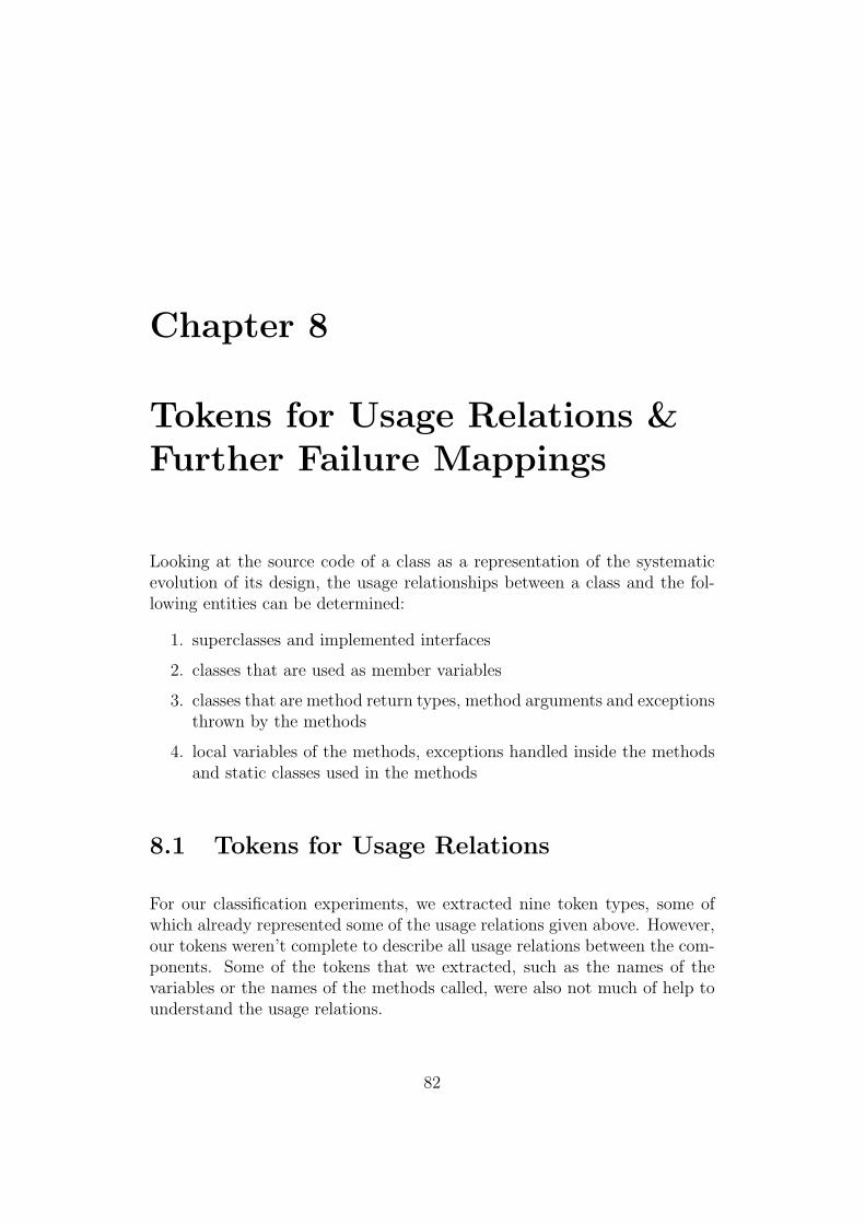
Chapter 8
Tokens for Usage Relations &Further Failure Mappings
Looking at the source code of a class as a representation of the systematicevolution of its design, the usage relationships between a class and the fol-lowing entities can be determined:
1. superclasses and implemented interfaces
2. classes that are used as member variables
3. classes that are method return types, method arguments and exceptionsthrown by the methods
4. local variables of the methods, exceptions handled inside the methodsand static classes used in the methods
8.1 Tokens for Usage Relations
For our classification experiments, we extracted nine token types, some ofwhich already represented some of the usage relations given above. However,our tokens weren’t complete to describe all usage relations between the com-ponents. Some of the tokens that we extracted, such as the names of thevariables or the names of the methods called, were also not much of help tounderstand the usage relations.
82

• Level 1 Tokens
• Level 2 Tokens
• Level 3 Tokens
• Level 4 Tokens
public class AntCorePlugin extends Plugin
implements IAntCoreConstants {...
private Map taskExtensions;
private AntCorePreferences preferences;
...
public void shutdown() throws CoreException {if (preferences == null)
return;
preferences.updatePluginPreferences();
savePluginPreferences();
}
private Map extractExtensions(String point, String key) {IExtensionPoint extensionPoint = null;
IConfigurationElement[ ] extensions = null;
extensionPoint = getDescriptor().getExtensionPoint(point);
if (extensionPoint == null)
return null;
extensions = extensionPoint.getConfigurationElements();
Map result = new HashMap(extensions.length);
...
return result;
}...
}
Table 8.1: Tokens in AntCorePlugin.java Source File
Under these circumstances, we decided to conduct a more detailed inspectionof Eclipse project for the new tokens. For a better illustration of the tokentypes collected in this new inspection, let’s reexamine the AntCorePlugin.javasource file from the previous chapter.
The colored parts of the code in Table 8.1 correspond to the tokens we
83

extracted for usage relations. For the naming of these tokens, we have usedthe names like ‘Level 1’ or ‘Level 4’, since those names represented the stageat which the relationships defined by the the tokens were defined during thedesign.
Level 1 Tokens: Level 1 tokens corresponded to the inheritance related to-kens from our initial token collection process. At this level, we collectedthe types of superclasses and the implemented interfaces for each class.
Level 2 Tokens: Level 2 tokens partially corresponded to the variable typetokens from the first part of our study. For our initial study, we col-lected types of variables inside a class, independent of their locations.For Level 2 tokens, we only examined the variable declarations of classmember variables. Primitive data types such as int and float weren’tincluded in these tokens.
Level 3 Tokens: As Level 3 tokens, from the method signatures, we col-lected the types of the arguments, the return types and the types ofthe exceptions that may be thrown by a method. Primitive data typeswere once again not taken into consideration.
Level 4 Tokens: Level 4 captured the remaining part of the variable typetokens, which isn’t covered by Level 2 and 3 tokens, by including thetypes of the local variables inside the methods. The types of exceptionswhich would be caught by a catch statement were also included in thistoken type.
Figure 8.1 demonstrates how we have considered the tokens from these levelsin our model building process. We have first used the tokens from Level 1,and later added the tokens from the upper levels. By this way, we aimed toobserve the effects of the evolution of the design process on the failures.
Figure 8.1: Different Levels of Usage Relations
84

In order to collect the information about new token types, we have used thebytecode of Java components rather than the source code. The main reasonbehind this decision was some difficulties that we have experienced in thestatic analysis with method argument bindings.
In the Java programming language, the bytecode is the form of instructionsthat the Java virtual machine (JVM) executes; and it is contained in the‘.class ’ files, which are the outcome of the compilation of source files (fileswith ‘.java’ extension) by the Java compiler. Each .class file contains thedefinition of a single class, or interface. Since the JVM is available on differentoperating systems, the same .class files can be executed on different systems,providing platform-independence to Java applications.
In order to collect the available tokens, we have used SIBRELIB, a softwarelibrary developed by Valentin Dallmeier, and ASM bytecode manipulationframework [2]. SIBRELIB library provided us with the functionality to ob-tain the bytecode representation of source files from .class files inside JARarchive files, whereas ASM framework supplied the means to parse the byte-code representation and access subfields such as the class definitions, classmember and local variable declarations, and method declarations. For each.class file, ASM framework also provided the name of the source file fromwhich the .class file was compiled. This allowed us to map classes back tosource files, and perform our experiments at source file level, as in the initialexperiments.
Although the analysis of bytecode made the extraction of the new token typeseasier, this approach also had some disadvantages. Unlike our initial tokenextraction method, this method couldn’t handle throw statements inside themethods (only ‘try-catch’ blocks could be tracked), and the accesses to staticvariables and methods couldn’t be observed as well. We believe that someof the usage relations defined by ‘throw’ tokens could have been capturedby ‘catch’ and ‘throws’ statements, which we had in our analysis. Althoughthose components whose members are statically accessed are parts of thegeneral usage relations, our new models couldn’t include those relations. Weaim to include the missing tokens into our analyses in our future work.
8.2 More Components with Failures
Like in the first part of our study, Schroter et al. [47] also investigated thefailures in release 2.0 and 2.1 of Eclipse project. However, they computedfailures for the individual entities differently. They checked whether
85

• Problem reports were submitted with six months after the release.
• Problem resolution field was set to “FIXED”.
• Severity of the problem had the value “CRITICAL”, “MAJOR”, or“NORMAL”.
Our initial data collection method differed in terms of the last step, whichdrops the failures of minor severity out of an investigation.
Another issue that was handled differently by Schroter et al. is the versionfields of the problem reports. A problem reported for a specific release maynot be fixed until the new release is deployed. In this case, the version numberwould be changed to the new release number, and once the failure is mappedto an entity, this failure would be counted for the new release. Taking thereport date for the problems into account, Schroter et al. took only thefirst reported version into account in which the report was reported. Webelieve that this approach gave better results about the number of failuresin a specific release of the Eclipse project.
The final difference between our and Schroter et al.’s failure mapping tech-niques was that, Schroter et al. also checked whether changes had beencommitted to the repository within a small period around the time pointat which a bug was resolved. Since this approach applied to those changeswhose log messages didn’t contain any phrases related to changes(‘Fixed ’,‘Bug ’), it provided more failure mappings than Sliwerski et al.’s method oflinking bugs and changes [49]. Schroter et al. [47] stated that, with this tech-nique, an additional 20% of failures in the Eclipse project were mapped tosome changes.
In light of these improvements, and, more importantly, to ensure the com-patibility between the results from Schroter et al.’s work and our new study,we decided to use the failure mappings made by Schroter et al. for the second
Figure 8.2: Mapping Failures to Correct Releases
86
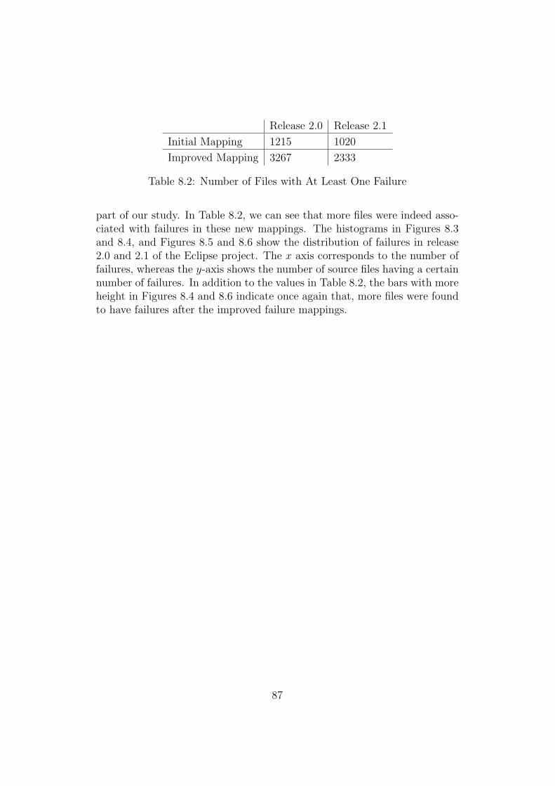
Release 2.0 Release 2.1
Initial Mapping 1215 1020
Improved Mapping 3267 2333
Table 8.2: Number of Files with At Least One Failure
part of our study. In Table 8.2, we can see that more files were indeed asso-ciated with failures in these new mappings. The histograms in Figures 8.3and 8.4, and Figures 8.5 and 8.6 show the distribution of failures in release2.0 and 2.1 of the Eclipse project. The x axis corresponds to the number offailures, whereas the y-axis shows the number of source files having a certainnumber of failures. In addition to the values in Table 8.2, the bars with moreheight in Figures 8.4 and 8.6 indicate once again that, more files were foundto have failures after the improved failure mappings.
87

Figure 8.3: Failure Frequencies in Eclipse Release 2.0 - Initial Mappings
Figure 8.4: Failure Frequencies in Eclipse Release 2.0 - Improved Mappings
88
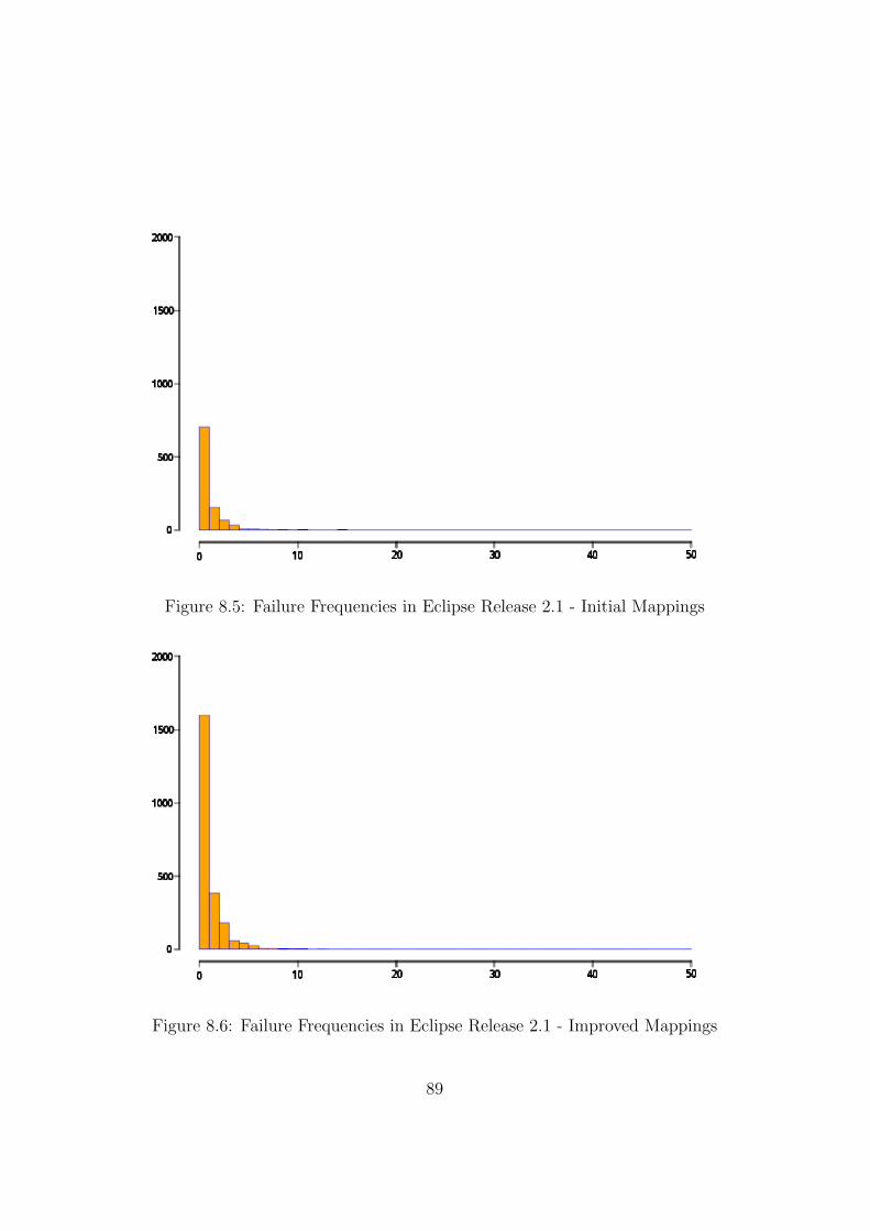
Figure 8.5: Failure Frequencies in Eclipse Release 2.1 - Initial Mappings
Figure 8.6: Failure Frequencies in Eclipse Release 2.1 - Improved Mappings
89
Chapter 9
Regression Models and Results
The information about the new token types, and the new failure mappingsin the Eclipse project were kept in the local databases. Even though theinput files for the regression experiments were created similar to those forthe classification experiments (the data in the two databases were joinedusing the file names, and suffix and deep suffix comparison methods), andthe regression models were created again using the R system; the experimentsin the second part of our study had some differences from the earlier ones,in terms of the input, and evaluation techniques.
9.1 Differences in Input
9.1.1 Failure Counts as Dependent Variable
The input data for the regression experiments had the structure given inFigure 9.1. Although the matrix structure stayed the same in the regressionexperiments, the first column of the matrix was used to represent the numberof the failures mapped to the entities, rather than their risk class. As thedependent variable, our models tried to predict the number of post-releasefailures instead of the risk classes.
90

Figure 9.1: Regression Experiments Input Format
9.1.2 Inputs at Fine and Coarse Granularities
One of the important observations we have made in the inputs of the classifi-cation experiments was that, the input matrices had a very sparse structure.Since there were various instances for different token types (i.e., more than2000 instances for inheritance tokens, as we have seen in Table 6.1), and thesource files generally contained tokens of only few of those instances; thissituation resulted in the matrices which contained many ‘0’ values. Havingexperienced this phenomenon, we decided to collect the instances and at-tributes under the packages, and perform our regression experiments at thepackage level as well.
At the package level, tokens from several instances/attributes were put to-gether, resulting in more compact instances/attributes sets, and therefore,less ‘0’ values in the input matrix. Besides these effects on the input ma-trices, changing the granularity for the instances helped us to see whetherwe can determine the problematic parts of a system at a larger scale, whichmay be used as a starting point before further investigations are made. Byexamining the attributes at the package level, we aimed to determine thepackages, the usage of which caused more risk.
Packages as Instances
To find the input values for the packages, we summed up the token and failurecounts from the individual source files. We believe that the input values atthe package level were correctly computed with this approach. The possibleproblem of overestimating the failure counts in the packages (demonstrated in
91
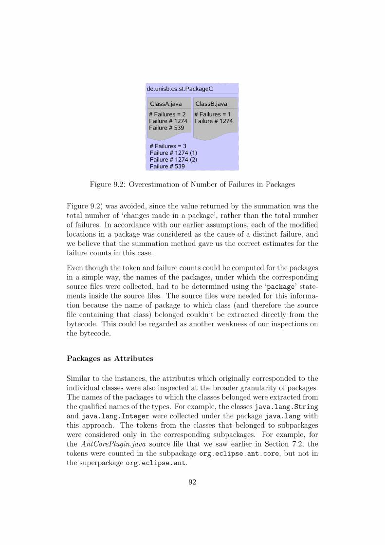
Figure 9.2: Overestimation of Number of Failures in Packages
Figure 9.2) was avoided, since the value returned by the summation was thetotal number of ‘changes made in a package’, rather than the total numberof failures. In accordance with our earlier assumptions, each of the modifiedlocations in a package was considered as the cause of a distinct failure, andwe believe that the summation method gave us the correct estimates for thefailure counts in this case.
Even though the token and failure counts could be computed for the packagesin a simple way, the names of the packages, under which the correspondingsource files were collected, had to be determined using the ‘package’ state-ments inside the source files. The source files were needed for this informa-tion because the name of package to which class (and therefore the sourcefile containing that class) belonged couldn’t be extracted directly from thebytecode. This could be regarded as another weakness of our inspections onthe bytecode.
Packages as Attributes
Similar to the instances, the attributes which originally corresponded to theindividual classes were also inspected at the broader granularity of packages.The names of the packages to which the classes belonged were extracted fromthe qualified names of the types. For example, the classes java.lang.Stringand java.lang.Integer were collected under the package java.lang withthis approach. The tokens from the classes that belonged to subpackageswere considered only in the corresponding subpackages. For example, forthe AntCorePlugin.java source file that we saw earlier in Section 7.2, thetokens were counted in the subpackage org.eclipse.ant.core, but not inthe superpackage org.eclipse.ant.
92

9.1.3 Excluding Project Independent Classes
In Java projects, the classes provided by the Java language are mostly usedmore often than the project specific classes. For example, the classes likejava.lang.String or java.io.Integer are used by many other classes and,therefore, occur more frequently inside the code.
Since, in our study, we aimed to determine the parts of “the Eclipse project”which were more open to mistakes, we wanted to eliminate the possible effectsof those project independent classes in our predictions. Therefore, we haveexcluded those token types (classes) coming from the Java language at thecorresponding levels (L - 2, L - 3, L - 4) and formed new sets of tokens (F - 2,F - 3, F - 4, where F stood for ‘filtered’). The tokens from Level 1 were keptout of this filtering, believing that the inheritance relations between classesaren’t as dense as other types of usage relations.
Table 9.1 shows, for each level of tokens, the number of files in release 2.0 fromwhich these tokens were extracted, and the number of distinct token instancesat each token level. Looking at the third and fifth columns of this table, wecan see that some token types were actually kept out of the examinationsafter the filtering. Comparing the numbers in the second and fourth columns,we can find that some of the files inside release 2.0 contained relationshipswith only those classes which were provided by the Java language. Thesefiles weren’t included in the experiments with the filtered token types. Tosee whether such changes in the attributes and instances had positive ornegative effects on the results, we have performed experiments with bothgroups of token sets.
In Section 6.4, we have explained that we had some problems with largeinput files and the requirements of the R system. Observing the number
# Files with # Distinct # Files with # DistinctToken Non-Empty Token Token Non-Empty TokenLevel Token Set Instances Level Token Set Instances
(Instances) (Features) (Instances) (Features)
L - 1 2181 4868 — — —L - 2 4342 5643 F - 2 4246 5186L - 3 4895 6339 F - 3 4706 5866L - 4 10498 6379 F - 4 10247 6197
Table 9.1: Distribution of Normal & Filtered Tokens in Eclipse Release 2.0
93

of instances and attributes in Table 9.1, one may naturally wonder how wecould perform the experiments with the inputs of these sizes, especially usingthe processing and storage resources provided by the moderate computermentioned in Section 6.4. In order to overcome the problems that we hadearlier, we performed our regression experiments on a super computer whichbecame available to us, as the second part of our study was conducted. Usingthe 32 GB main memory, and 64-bit, 2 GHz dual-core processors of thiscomputer, we were able to perform our experiments without problems.
9.2 Differences in Evaluation
9.2.1 Random Splitting and Complement Method
In the classification experiments, we have evaluated our models using thecross-validation and the complement methods. For the regression models, wehave applied random data splitting technique combined with the complementmethod, as it was used by Schroter et al. [47].
In Section 4.1, we have mentioned that the functionality of Eclipse projectdepends on smaller components called plug-ins. For the regression experi-ments we have performed the random-splitting method at the plug-in level,and splitted the plug-ins of Eclipse release 2.0 randomly into training andtesting groups. To determine the complete set of plug-ins available in ourstudy, for each source file in our token database, we have determined whichEclipse plug-in it belonged to, by simply taking the corresponding plug-inname out of the file path.
release20/plug-ins/org.eclipse.ant.core/org/. . . /AntRunner.java
After finding the set of available plug-ins, we have selected one third of therelease 2.0 plug-ins as the training set, and the remaining two thirds as thetesting set for release 2.0, following Schroter et al.’s techniques [47]. As wecan see in Figure 9.3, after the plug-ins were determined and separated, thedata from those files of release 2.0, whose plug-ins were placed in the traininggroup, formed the training data set. The data from the remaining files ofrelease 2.0 was put into the testing data set for release 2.0. The plug-insof release 2.1 which weren’t put into the training group formed the testinggroup of release 2.1. The files in this group were handled similarly to thosefrom release 2.0.
94

Figure 9.3: Data Splitting Combined with Complement Method
In the regression experiments, by keeping the ratio of the training instancessmaller (the usual division of samples is two thirds for training and onethird for testing), it became also possible to see whether our models wouldmake good predictions, and whether we could use the models early in thedevelopment process, without waiting for complete releases to finish. Sincefewer instances were involved in the training process, in order to be able toconsider all instances in some training case, and also to have compatabilitybetween our results and those from Schroter et al. [47], we have applied ourseparation and model building process 40 times. Unlike the cross-validationmethod which determined the subsets once at the beginning, and later usedthem without any changes; the training and testing sets were determinedrandomly at each iteration of the random splitting approach.
9.2.2 Riskiness Rankings
In the first part of our study, we aimed to determine which components shouldbe considered as ‘risky’. The same goal of risk classification of componentscontinued in the regression models, and we used once again the precision andrecall values to assess our models.
With the predicted failure counts for the components, we were able to makean ordering of the components as well as a risk classification. The components
95

File # Failures # Failures Rank RankName (Real) (Predicted) (Real) (Predicted)
A.java 3 6 3 3B.java 10 12 1 1C.java 1 2 4 4D.java 0 1 5 5E.java 5 8 2 2
Table 9.2: Rank Correlation Example
were sorted according to the predicted failure counts, and the top elementsin this ordering (ranking) were the components which were defined to be themost-risky by the models. Based on the original failure counts, we obtaineda second ranking, and we compared these two rankings using Spearman rankcorrelation.
Correlation is a statistical technique which shows whether and how stronglypairs of variables are linearly related. It tells how much two variables, Xand Y , tend to vary together. Correlation takes values in the range [−1, 1]and high positive values show that the increase in X comes with an increasein Y . Low negative values indicate that just the opposite situation is valid,such that X values increase, while Y values decrease. A correlation value of‘0’ indicates that there is no linear relation between the variables.
In the rank correlation, a rank order is given to the instances of each variableand the correlation values for the ranks are computed. Similar to correlation,the value ‘1’ represents a perfect agreement in the rankings (rankings ineach pair are the same), whereas ‘−1’ value shows that one ranking is thereverse of the other one. Once again, ‘0’ values indicate that the rankings areindependent. In Table 9.2, we see that the rankings are the same for everycase, giving a rank correlation of value ‘1’.
Spearman rank correlation coefficient, ρ, is computed as
ρ = 1 −6
∑D2
N(N2 − 1)
where D is the difference between the ranks of corresponding X and Y valuesand N is the number of pairs of values. Spearman rank correlation makesno assumptions about the frequency distribution of the variables (normallydistributed variables), or the linear relationship between the variables.
96
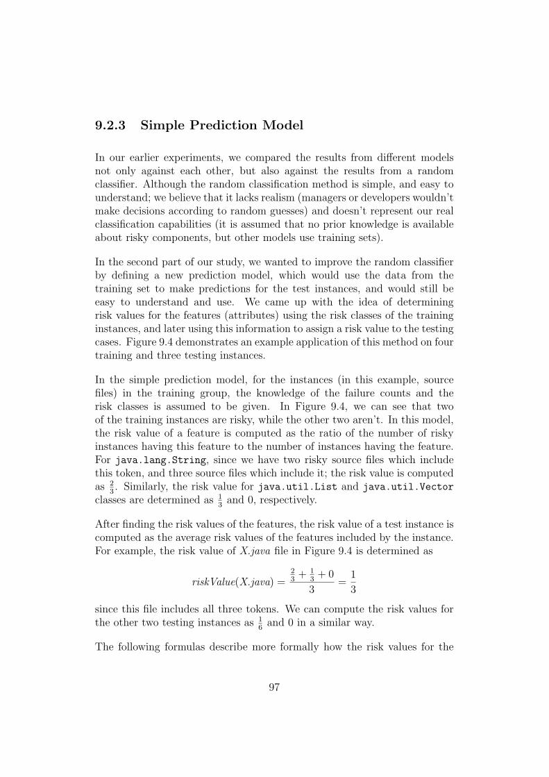
9.2.3 Simple Prediction Model
In our earlier experiments, we compared the results from different modelsnot only against each other, but also against the results from a randomclassifier. Although the random classification method is simple, and easy tounderstand; we believe that it lacks realism (managers or developers wouldn’tmake decisions according to random guesses) and doesn’t represent our realclassification capabilities (it is assumed that no prior knowledge is availableabout risky components, but other models use training sets).
In the second part of our study, we wanted to improve the random classifierby defining a new prediction model, which would use the data from thetraining set to make predictions for the test instances, and would still beeasy to understand and use. We came up with the idea of determiningrisk values for the features (attributes) using the risk classes of the traininginstances, and later using this information to assign a risk value to the testingcases. Figure 9.4 demonstrates an example application of this method on fourtraining and three testing instances.
In the simple prediction model, for the instances (in this example, sourcefiles) in the training group, the knowledge of the failure counts and therisk classes is assumed to be given. In Figure 9.4, we can see that twoof the training instances are risky, while the other two aren’t. In this model,the risk value of a feature is computed as the ratio of the number of riskyinstances having this feature to the number of instances having the feature.For java.lang.String, since we have two risky source files which includethis token, and three source files which include it; the risk value is computedas 2
3. Similarly, the risk value for java.util.List and java.util.Vector
classes are determined as 13
and 0, respectively.
After finding the risk values of the features, the risk value of a test instance iscomputed as the average risk values of the features included by the instance.For example, the risk value of X.java file in Figure 9.4 is determined as
riskValue(X.java) =23
+ 13
+ 0
3=
1
3
since this file includes all three tokens. We can compute the risk values forthe other two testing instances as 1
6and 0 in a similar way.
The following formulas describe more formally how the risk values for the
97

features, f, and the instances, i, are calculated.
riskValue(f) =
∑
i∈TrainingSetisRisky(i)
|{i : i ∈ TrainingSet ∧ f ∈ features(i)}|
riskValue(i) =
∑
f∈features(i)riskValue(f)
|{f : f ∈ features(i)}|
isRisky function in the numerator returns ‘1’ if the given argument instancei is risky and ‘0’ if not. features function returns the set of features (at-tributes) which the instance possesses (features with positive values in thecorresponding columns of the data matrix).
According to these equations, the risk value for the tokens increase if moreof the risky components in the training set contain those tokens. For thecomponents in the testing set, the riskier classes or interfaces the componentsuse; riskier they become.
Figure 9.4: Simple Prediction Model Example
98

In the simple prediction model, the risk values for the features and the in-stances lie always between ‘0’ and ‘1’, so we used the models built with thisapproach for classification purposes. We used the threshold value of ‘0.5’ todetermine the risk classes of files and packages. Since we considered packageswith at least one failure as risky while determining the original risk classes;we decided to take the maximum of the risk values from the source files in apackage as the package’s risk value. The thresholding technique was appliedon this maximum value.
9.3 Building Regression Models
The linear regression models used in the second part of our study were builtonce again by using the functions provided by the R-system with the defaultparameters. The support vector models were built in the regression setup,using the radial basis kernel. To assure compatability, the parameters forthis kernel had the same values as the parameters from Schroter et al.’sSVM models.
Since the predictions from the linear regression and SVM models weren’trestricted to the [0,1] interval, we set the threshold value for the risk classi-fication to ‘0’. So the instances with positive predicted failure counts wereclassified as risky.
9.4 Results from Regression Experiments
As we have mentioned at the beginning of this chapter, we have conductedexperiments at four different input granularities: source files/packages asinstances, and classes/packages as features. The precision-recall graphs andtables in the following sections show the results in each input setting, togetherfor the release 2.0 and 2.1 testing data.
In each section, the tables following the precision-recall graphs hold the infor-mation about three other evaluation measures: Spearman rank correlationvalue, the rank correlation and precision values for the top-5% of compo-nents in the predicted rankings. The precision and rank correlation valuesfor the top ranked components were computed at different percentages (5%,10%, 15%, 20%) to see whether the components which were predicted to be
99

most-risky were actually risky, and whether the failure-based ordering of thetop ranked components were correct. Due to the space limitations, the rankcorrelation and precision values for only the top-5% of the components aregiven in the following sections. The complete results for the experiments canbe found in the Appendix.
9.4.1 Files as Instances and Classes as Features
Linear Regression
The results in Figure 9.5 show that the linear regression models had higherprecision and lower recall values than the random classifier. The precisionvalues for the release 2.1 testing set were lower than the values for the release2.0 set, showing a similar structure to what we had seen in the classificationexperiments. When higher token levels were considered in the models, themodels covered more of the risky files, but they also made more mistakes atdifferentiating between risky and not-risky files.
As we can see in Table 9.3, the precision values for the top risky files werehigher than the values for the whole testing sets. As the token level increased,the top-5% precision values increased as well. At the end, the models werearound 10 - 15% more precise than the random classification strategy, whichwas a clear improvement.
One of the interesting points in Table 9.3 was the relatively high Spearmanrank correlation values for some models, especially those built on filteredtokens data. Despite the high correlation values for the whole testing sets,the correlation values were close to ‘0’ for the top ranked files. Our firstexplanation for this situation was that, the not-risky files, which formed themajority of the testing set and were collected at the bottom of the rankings,might have increased the rank correlations for the whole model; whereas therankings of the risky files didn’t correlate with the real rankings.
Support Vector Machines
At the fine granularity of both instances and attributes, the SVM modelsfailed to make a proper classification with the first two levels of tokens. Forthese token types, in some of the 40 iterations, the models classified all source
100

Figure 9.5: Precision-Recall Values for Linear Regression Models (Instances:Files, Features: Classes)
Level Spear. Spear. Prec. Level Spear. Spear. Prec.Top-5% Top-5% Top-5% Top-5%
Rel.2.0
L1 0.5221 -0.0135 0.3059 — — — —
L2 0.4465 0.0148 0.3421 F2 0.4722 -0.0936 0.3509
L3 0.2754 0.0449 0.3742 F3 0.4913 0.0030 0.3643
L4 0.2955 0.0268 0.4140 F4 0.4979 -0.0054 0.4243
Rel.2.1
L1 0.5679 -0.0587 0.2630 — — — —
L2 0.3240 0.0133 0.2440 F2 0.5731 -0.0863 0.2511
L3 0.2787 0.0575 0.2611 F3 0.3024 0.0261 0.2613
L4 0.2833 0.0272 0.2387 F4 0.3302 0.0123 0.2625
Table 9.3: Spearman, Top-5% Spearman, and Top-5% Precision Values forLinear Regression Models (Instances: Files, Features: Classes)
101
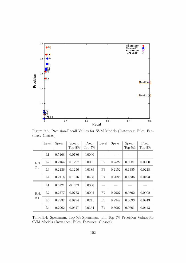
Figure 9.6: Precision-Recall Values for SVM Models (Instances: Files, Fea-tures: Classes)
Level Spear. Spear. Prec. Level Spear. Spear. Prec.Top-5% Top-5% Top-5% Top-5%
Rel.2.0
L1 0.5468 0.0786 0.0000 — — — —
L2 0.2164 0.1297 0.0001 F2 0.2522 0.0981 0.0000
L3 0.2136 0.1256 0.0189 F3 0.2152 0.1355 0.0228
L4 0.2116 0.1316 0.0408 F4 0.2088 0.1336 0.0493
Rel.2.1
L1 0.3721 -0.0121 0.0000 — — — —
L2 0.2777 0.0773 0.0002 F2 0.2927 0.0862 0.0002
L3 0.2937 0.0794 0.0241 F3 0.2942 0.0693 0.0243
L4 0.2962 0.0527 0.0354 F4 0.3002 0.0601 0.0413
Table 9.4: Spearman, Top-5% Spearman, and Top-5% Precision Values forSVM Models (Instances: Files, Features: Classes)
102

files as not-risky, and the precision values couldn’t be computed in thoseiterations. In order to be able to compute the average precision values, we hadto specially handle these cases, and we decided to take the precision valuesas ‘0’, and to keep these iterations in the average computation. Although theaverages of only positive values could have also been taken, or the precisionvalues for the problematic cases could have also been counted as ‘1’ instead of‘0’ (since no prediction was made about riskiness, the model could have beenregarded as very precise, as well); we believed that keeping the problematiccases in the average computation with ‘0’ values could be taken as a form of“penalizing” these models for the misclassifications.
As it can be seen in Figure 9.6, the SVM models gave better precision val-ues with the increasing levels of tokens and with the filtered token types.However, the recall values didn’t increase with more attributes. Our exam-inations showed that, even in the models which gave reasonable results interms of precision, very few risky files and a few more not-risky files hadbeen classified as risky. Such a distribution in the results caused the decep-tively good precision values, but the recall values helped us to see the realsituation.
In Table 9.4, we see that the correlation values both for the whole test setsand for the top ranked components weren’t as good as the ones from thelinear regression models, whereas the precision values for the componentsclassified as most-risky were very low. Since only very few risky files wereclassified correctly, this situation also affected the precision values at top-5%levels.
Simple Prediction
In Figure 9.7, we have the precision and recall values for the simple predictionmodel in the first experiment setup. Although our simple prediction modelshad better precision values than the random classifier in general, the recallvalues were very low. In this input setting, there were also no clear effectsof the introduction of tokens from higher levels. We believed that, since thesimple model took the non-weighted averages of the risk values; the modelsmight have not responded to the usage relations intensifying at higher levels.The insertion of tokens from non-project classes had no significant effects onthe results, probably due to the same reason.
Unlike the top-5% precision values from linear regresion and SVM models, theprecision values for the most risky files in the simple prediction models were
103
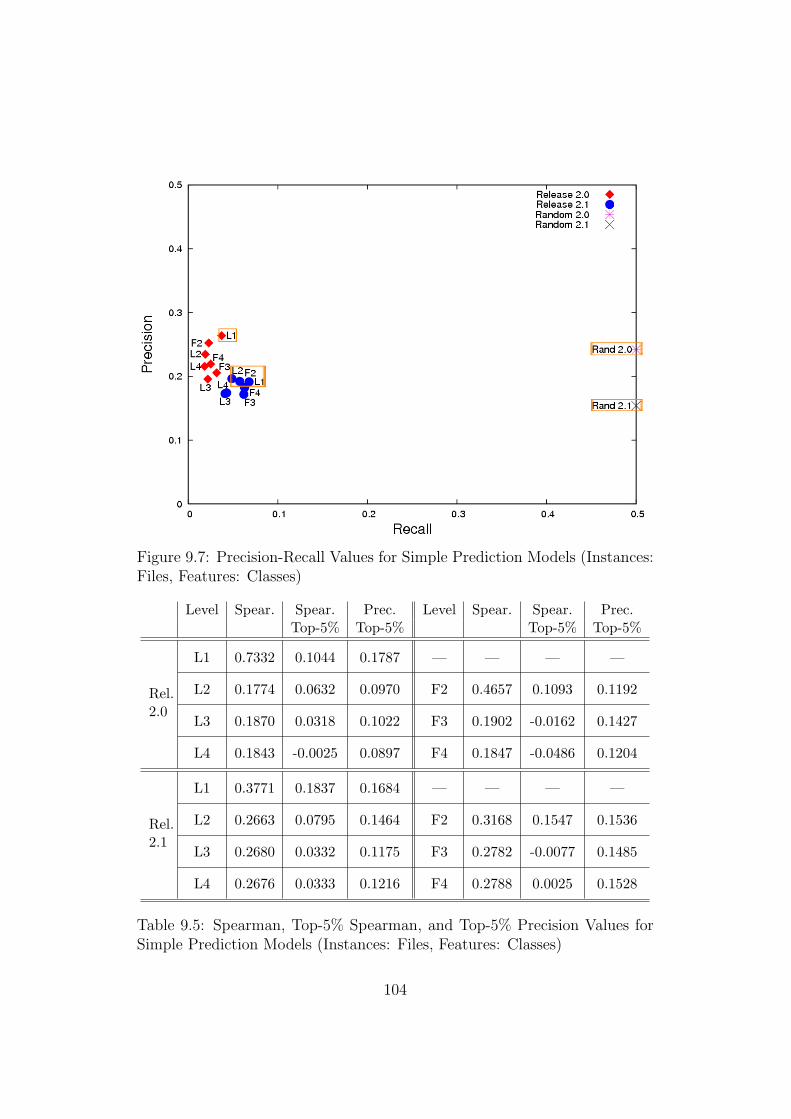
Figure 9.7: Precision-Recall Values for Simple Prediction Models (Instances:Files, Features: Classes)
Level Spear. Spear. Prec. Level Spear. Spear. Prec.Top-5% Top-5% Top-5% Top-5%
Rel.2.0
L1 0.7332 0.1044 0.1787 — — — —
L2 0.1774 0.0632 0.0970 F2 0.4657 0.1093 0.1192
L3 0.1870 0.0318 0.1022 F3 0.1902 -0.0162 0.1427
L4 0.1843 -0.0025 0.0897 F4 0.1847 -0.0486 0.1204
Rel.2.1
L1 0.3771 0.1837 0.1684 — — — —
L2 0.2663 0.0795 0.1464 F2 0.3168 0.1547 0.1536
L3 0.2680 0.0332 0.1175 F3 0.2782 -0.0077 0.1485
L4 0.2676 0.0333 0.1216 F4 0.2788 0.0025 0.1528
Table 9.5: Spearman, Top-5% Spearman, and Top-5% Precision Values forSimple Prediction Models (Instances: Files, Features: Classes)
104

lower than the precision values computed for the whole testing instances.This showed that the models were precise in general but not particularlyfor the most risky instances. The Spearman correlation values in Table 9.5indicated that the rankings for some models were very successful, while thecorrelation rates dropped rapidly in the top-5% of the files, similar to whatwe have seen in the other models. However, the high rank correlation valuesin third and seventh columns of Table 9.5 made us believe that, the recalland maybe the precision values of some models could have been improvedwith a different threshold value.
9.4.2 Files as Instances and Packages as Features
Linear Regression
Unlike the results from the first type of experiments, we didn’t have a specificpattern for the precision and recall values with the broader granularity ofinstances, as we can also see in Figure 9.8. Instead, our models gave recallvalues which were much higher than those from the random classifier.
After becoming suspicious about the relatively high recall values which wereaccompanied by the low precision values, we checked the results from the in-dividual iterations. Our inspections showed that the linear regression modelsclassified most of the instances in testing sets as risky. From Table 9.6, wecan see that, among the most risky files, we had less not-risky files that wereclassified incorrectly, resulting in the precision values which were higher thanthose computed for the complete test sets.
When compared with the correlations values from Table 9.3, the correlationvalues in the second input setup were lower. Yet, thinking that the modelshad made many misclassifications in this experiment setting, the lack ofcorrelation in testing sets and among the top ranked files could be consideredas normal.
Support Vector Machines
The precision and recall values for SVM models in Figure 9.9 showed thatthe SVM models experienced once again major misclassification problems.The precision values which were similar to those from the random classifier,
105
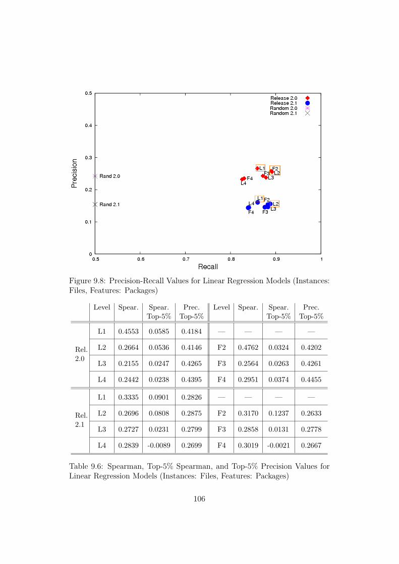
Figure 9.8: Precision-Recall Values for Linear Regression Models (Instances:Files, Features: Packages)
Level Spear. Spear. Prec. Level Spear. Spear. Prec.Top-5% Top-5% Top-5% Top-5%
Rel.2.0
L1 0.4553 0.0585 0.4184 — — — —
L2 0.2664 0.0536 0.4146 F2 0.4762 0.0324 0.4202
L3 0.2155 0.0247 0.4265 F3 0.2564 0.0263 0.4261
L4 0.2442 0.0238 0.4395 F4 0.2951 0.0374 0.4455
Rel.2.1
L1 0.3335 0.0901 0.2826 — — — —
L2 0.2696 0.0808 0.2875 F2 0.3170 0.1237 0.2633
L3 0.2727 0.0231 0.2799 F3 0.2858 0.0131 0.2778
L4 0.2839 -0.0089 0.2699 F4 0.3019 -0.0021 0.2667
Table 9.6: Spearman, Top-5% Spearman, and Top-5% Precision Values forLinear Regression Models (Instances: Files, Features: Packages)
106

Figure 9.9: Precision-Recall Values for SVM Models (Instances: Files, Fea-tures: Packages)
Level Spear. Spear. Prec. Level Spear. Spear. Prec.Top-5% Top-5% Top-5% Top-5%
Rel.2.0
L1 0.4271 0.0086 0.4360 — — — —
L2 0.2232 0.0545 0.4574 F2 0.2323 0.0714 0.4701
L3 0.2238 0.1189 0.4819 F3 0.2292 0.1375 0.4946
L4 0.2263 0.0869 0.5149 F4 0.2271 0.0983 0.5307
Rel.2.1
L1 0.3554 0.0268 0.2720 — — — —
L2 0.2879 0.0820 0.2980 F2 0.2993 0.0879 0.3029
L3 0.3098 0.1019 0.2662 F3 0.3099 0.1025 0.2717
L4 0.3237 0.0356 0.3206 F4 0.3241 0.0314 0.3302
Table 9.7: Spearman, Top-5% Spearman, and Top-5% Precision Values forSVM Models (Instances: Files, Features: Packages)
107

and the recall values that were very close to ‘1’ made us believe that themodels might have classified most files to be risky. The inspections on theresults from the individual iterations showed that this was indeed the case.
Despite the misclassifications, the precision values from Table 9.7 indicatedthat the models were able to distinguish between risky and not-risky filesmore successfully among the files which were predicted to be the most risky.Although the predicted rankings for the top risky files showed small simi-larities with the original rankings, the Spearman correlation values for thecomplete sets indicated that the SVM models were still able to make a dis-tinction of which source files were more risky than the others in the generalsense (since most files were classified as risky, it wasn’t possible to relatethe correlation values with the not-risky files which would have lower ranksunder normal circumstances).
Simple Prediction
The precision and recall values for the simple prediction models in Figure 9.10showed a pattern similar to that observed in Figure 9.7. Even though theprecision values for the models with Level L1 tokens were slightly higherthan those from the random classifier, the simple prediction models lackedonce again the high recall values. The help of filtered token types in termsof recall was also very small. The similar results observed in Figures 9.7and 9.10 raised the question of whether the risk values of the classes from asingle package might have showed similar risk characteristics.
The Spearman correlation values in Table 9.8 showed that the simple pre-diction model was able to give a better ranking in release 2.1. However, inboth test data sets, the rank correlations for the top-5% of files were lowerthan the values for the complete models, which indicated that the the topportion of the rankings weren’t very helpful to determine which source filesshould be examined first in the development.
9.4.3 Packages as Instances and Classes as Features
Linear Regression
As it can be seen in Figure 9.11, the linear regression models had both betterprecision and recall values than the random classifier for release 2.1 set. In
108
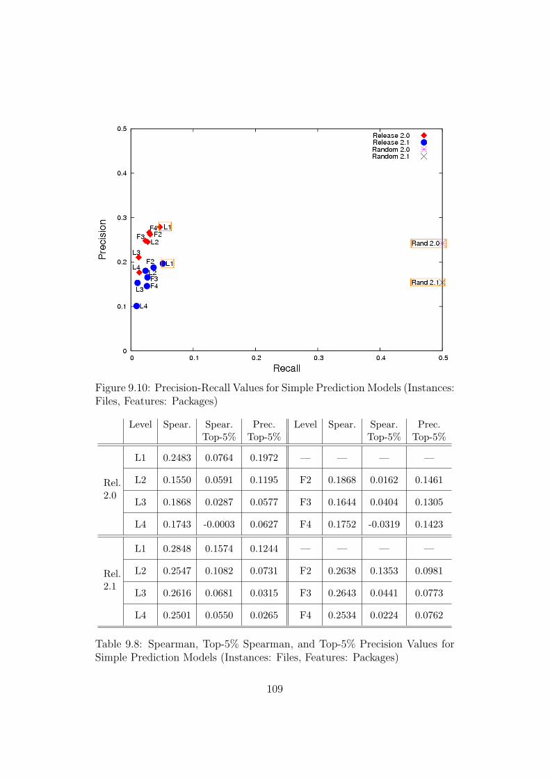
Figure 9.10: Precision-Recall Values for Simple Prediction Models (Instances:Files, Features: Packages)
Level Spear. Spear. Prec. Level Spear. Spear. Prec.Top-5% Top-5% Top-5% Top-5%
Rel.2.0
L1 0.2483 0.0764 0.1972 — — — —
L2 0.1550 0.0591 0.1195 F2 0.1868 0.0162 0.1461
L3 0.1868 0.0287 0.0577 F3 0.1644 0.0404 0.1305
L4 0.1743 -0.0003 0.0627 F4 0.1752 -0.0319 0.1423
Rel.2.1
L1 0.2848 0.1574 0.1244 — — — —
L2 0.2547 0.1082 0.0731 F2 0.2638 0.1353 0.0981
L3 0.2616 0.0681 0.0315 F3 0.2643 0.0441 0.0773
L4 0.2501 0.0550 0.0265 F4 0.2534 0.0224 0.0762
Table 9.8: Spearman, Top-5% Spearman, and Top-5% Precision Values forSimple Prediction Models (Instances: Files, Features: Packages)
109

Figure 9.11: Precision-Recall Values for Linear Regression Models (Instances:Packages, Features: Files)
Level Spear. Spear. Prec. Level Spear. Spear. Prec.Top-5% Top-5% Top-5% Top-5%
Rel.2.0
L1 0.0179 -0.0656 0.7975 — — — —
L2 0.0835 -0.0300 0.8107 F2 0.0111 0.0655 0.8198
L3 0.0548 0.0636 0.7991 F3 0.0027 -0.0524 0.8407
L4 0.0443 -0.0901 0.7884 F4 0.0054 -0.0443 0.8143
Rel.2.1
L1 0.0670 -0.0275 0.7718 — — — —
L2 0.1009 -0.0353 0.7731 F2 0.0162 -0.0019 0.7440
L3 0.0806 0.0063 0.7694 F3 0.0365 -0.0472 0.7625
L4 0.0752 0.0107 0.7765 F4 0.0480 -0.0389 0.7664
Table 9.9: Spearman, Top-5% Spearman, and Top-5% Precision Values forLinear Regression Models (Instances: Packages, Features: Files)
110

both testing sets, the recall values for the linear regression models were better.The decrease in the recall values with the additional features was observedin this experiment setting, too.
Different from those from the earlier experiments, the Spearman correlationvalues in Table 9.9 were close to ‘0’, both for whole packages and top riskyones. This indicated that the ordering made by the linear regression modelswouldn’t be much of use for this input type. However, the precision valuesfor the top-5% of the packages were high and quite reliable, such that inalmost eight out of ten cases where the models classified a package as risky,the decisions were right.
Support Vector Machines
The precision and recall values for the SVM models in Figure 9.12 had adistribution similar to those from Figure 9.9. With the instances given aspackages, the SVM models had once again difficulties at making a properclassification of the instances. While most of the risky and not-risky pack-ages were classified as risky in release 2.0 (also with some risky packagesclassified as not-risky); in release 2.1 testing set, fewer not-risky packageswere classified incorrectly, resulting in higher precision values. In Table 9.10,we can see that the SVM models had high precision values for top-5% of thepackages, indicating that the models assigned higher failure counts to thereal risky packages.
As we can understand from the precision values of the random classificationmodels in Figure 9.9, the rate of risky packages in the testing sets were around65% and 45%. Especially with more packages being risky in release 2.0, theSVM models had relatively high Spearman correlation values. We believethat such high Spearman correlation values may have been a result of themisclassifications, and the general riskiness trend in the testing sets.
Simple Prediction
In the third set of regression experiments, the simple prediction models hadonce again higher precision and lower recall values than the random models.As we can see in Figure 9.13, especially the models in release 2.1 set were veryprecise, compared with the random classifier. The recall values decreasedand the precision values increased as more token types were added into our
111
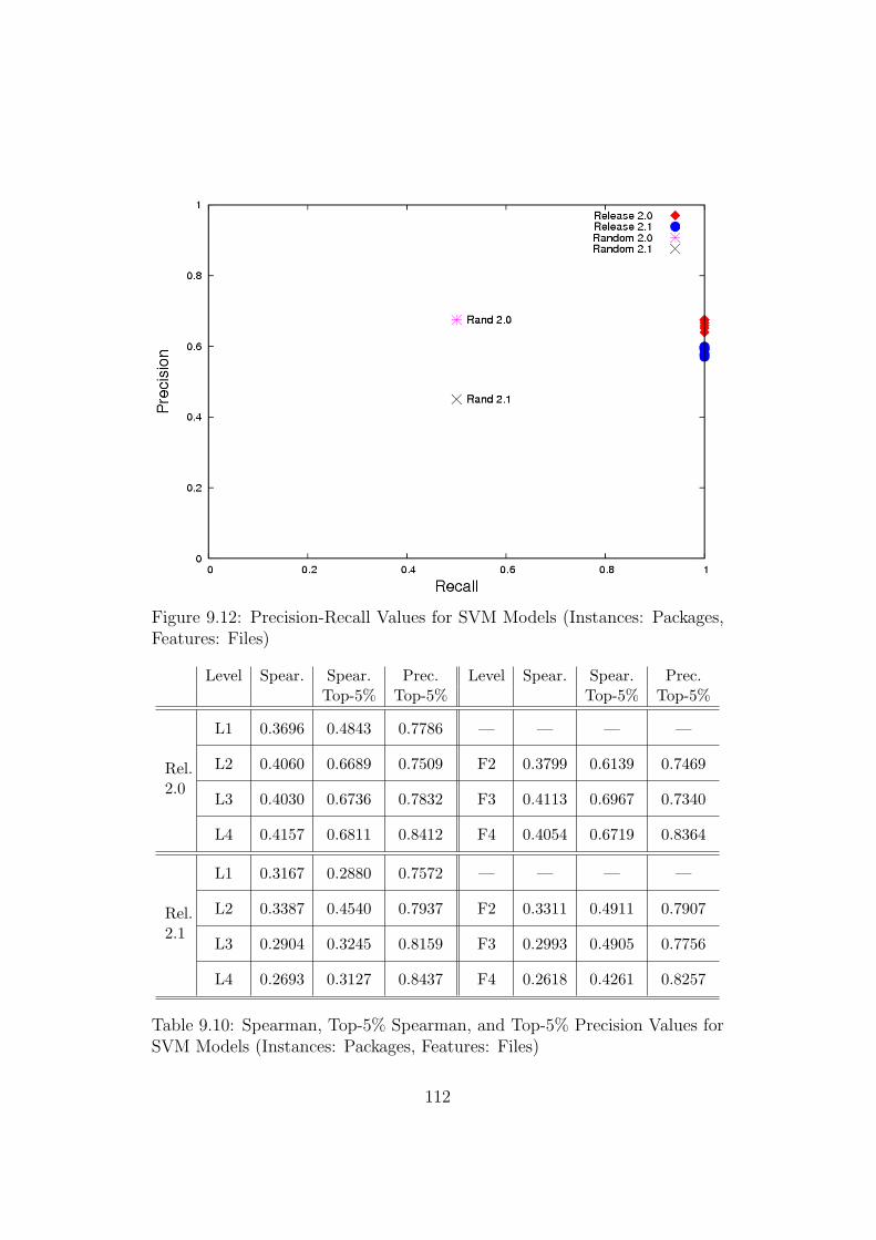
Figure 9.12: Precision-Recall Values for SVM Models (Instances: Packages,Features: Files)
Level Spear. Spear. Prec. Level Spear. Spear. Prec.Top-5% Top-5% Top-5% Top-5%
Rel.2.0
L1 0.3696 0.4843 0.7786 — — — —
L2 0.4060 0.6689 0.7509 F2 0.3799 0.6139 0.7469
L3 0.4030 0.6736 0.7832 F3 0.4113 0.6967 0.7340
L4 0.4157 0.6811 0.8412 F4 0.4054 0.6719 0.8364
Rel.2.1
L1 0.3167 0.2880 0.7572 — — — —
L2 0.3387 0.4540 0.7937 F2 0.3311 0.4911 0.7907
L3 0.2904 0.3245 0.8159 F3 0.2993 0.4905 0.7756
L4 0.2693 0.3127 0.8437 F4 0.2618 0.4261 0.8257
Table 9.10: Spearman, Top-5% Spearman, and Top-5% Precision Values forSVM Models (Instances: Packages, Features: Files)
112
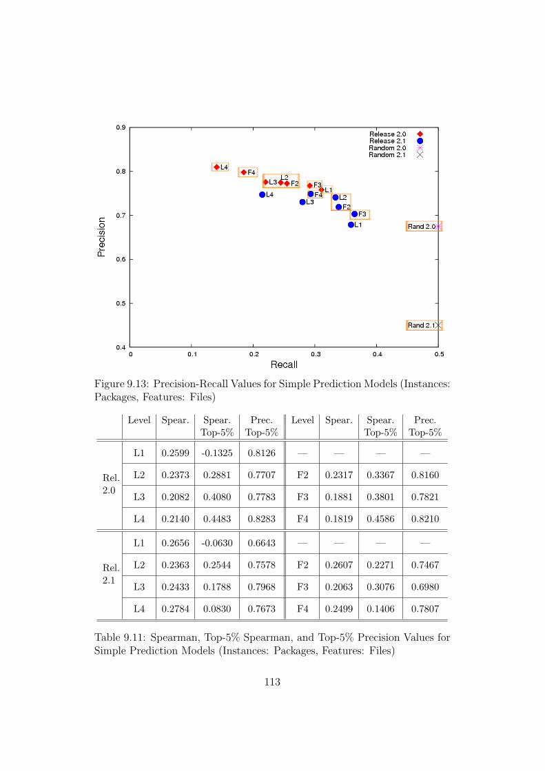
Figure 9.13: Precision-Recall Values for Simple Prediction Models (Instances:Packages, Features: Files)
Level Spear. Spear. Prec. Level Spear. Spear. Prec.Top-5% Top-5% Top-5% Top-5%
Rel.2.0
L1 0.2599 -0.1325 0.8126 — — — —
L2 0.2373 0.2881 0.7707 F2 0.2317 0.3367 0.8160
L3 0.2082 0.4080 0.7783 F3 0.1881 0.3801 0.7821
L4 0.2140 0.4483 0.8283 F4 0.1819 0.4586 0.8210
Rel.2.1
L1 0.2656 -0.0630 0.6643 — — — —
L2 0.2363 0.2544 0.7578 F2 0.2607 0.2271 0.7467
L3 0.2433 0.1788 0.7968 F3 0.2063 0.3076 0.6980
L4 0.2784 0.0830 0.7673 F4 0.2499 0.1406 0.7807
Table 9.11: Spearman, Top-5% Spearman, and Top-5% Precision Values forSimple Prediction Models (Instances: Packages, Features: Files)
113
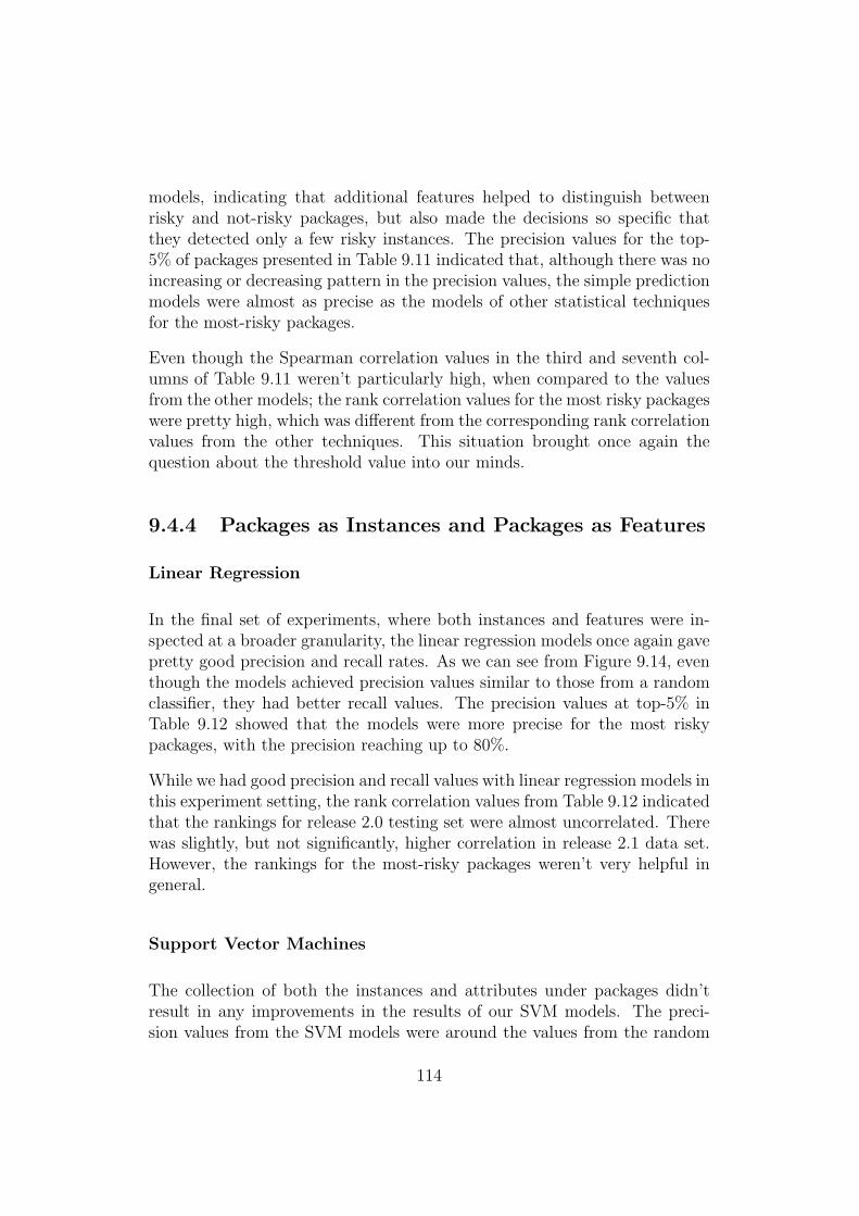
models, indicating that additional features helped to distinguish betweenrisky and not-risky packages, but also made the decisions so specific thatthey detected only a few risky instances. The precision values for the top-5% of packages presented in Table 9.11 indicated that, although there was noincreasing or decreasing pattern in the precision values, the simple predictionmodels were almost as precise as the models of other statistical techniquesfor the most-risky packages.
Even though the Spearman correlation values in the third and seventh col-umns of Table 9.11 weren’t particularly high, when compared to the valuesfrom the other models; the rank correlation values for the most risky packageswere pretty high, which was different from the corresponding rank correlationvalues from the other techniques. This situation brought once again thequestion about the threshold value into our minds.
9.4.4 Packages as Instances and Packages as Features
Linear Regression
In the final set of experiments, where both instances and features were in-spected at a broader granularity, the linear regression models once again gavepretty good precision and recall rates. As we can see from Figure 9.14, eventhough the models achieved precision values similar to those from a randomclassifier, they had better recall values. The precision values at top-5% inTable 9.12 showed that the models were more precise for the most riskypackages, with the precision reaching up to 80%.
While we had good precision and recall values with linear regression models inthis experiment setting, the rank correlation values from Table 9.12 indicatedthat the rankings for release 2.0 testing set were almost uncorrelated. Therewas slightly, but not significantly, higher correlation in release 2.1 data set.However, the rankings for the most-risky packages weren’t very helpful ingeneral.
Support Vector Machines
The collection of both the instances and attributes under packages didn’tresult in any improvements in the results of our SVM models. The preci-sion values from the SVM models were around the values from the random
114

Figure 9.14: Precision-Recall Values for Linear Regression Models (Instances:Packages, Features: Packages)
Level Spear. Spear. Prec. Level Spear. Spear. Prec.Top-5% Top-5% Top-5% Top-5%
Rel.2.0
L1 0.1303 0.1399 0.8054 — — — —
L2 0.0254 -0.0064 0.7274 F2 0.0444 -0.0906 0.7823
L3 0.0261 0.0105 0.7552 F3 0.0157 -0.0446 0.7574
L4 0.0363 0.0858 0.8028 F4 0.0220 0.0020 0.8273
Rel.2.1
L1 0.3210 0.0059 0.7036 — — — —
L2 0.2734 0.0246 0.7079 F2 0.2996 0.0090 0.7274
L3 0.2525 0.0594 0.7113 F3 0.2480 -0.0204 0.6911
L4 0.2409 -0.0226 0.6485 F4 0.2129 -0.0427 0.6679
Table 9.12: Spearman, Top-5% Spearman, and Top-5% Precision Values forLinear Regression Models (Instances: Packages, Features: Packages)
115

Figure 9.15: Precision-Recall Values for SVM Models (Instances: Packages,Features: Packages)
Level Spear. Spear. Prec. Level Spear. Spear. Prec.Top-5% Top-5% Top-5% Top-5%
Rel.2.0
L1 0.4199 0.4145 0.8629 — — — —
L2 0.4261 0.3463 0.7809 F2 0.4294 0.3546 0.7763
L3 0.3521 0.0655 0.7930 F3 0.3593 0.0621 0.7873
L4 0.2125 0.0933 0.8271 F4 0.2087 0.1044 0.8252
Rel.2.1
L1 0.2013 0.1938 0.8381 — — — —
L2 0.2028 -0.0983 0.8107 F2 0.2122 0.0366 0.8072
L3 0.1794 -0.1807 0.5900 F3 0.1752 -0.0872 0.5694
L4 0.2002 -0.0740 0.5662 F4 0.1897 -0.0098 0.5609
Table 9.13: Spearman, Top-5% Spearman, and Top-5% Precision Values forSVM Models (Instances: Packages, Features: Packages)
116
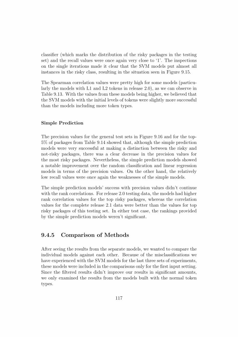
classifier (which marks the distribution of the risky packages in the testingset) and the recall values were once again very close to ‘1’. The inspectionson the single iterations made it clear that the SVM models put almost allinstances in the risky class, resulting in the situation seen in Figure 9.15.
The Spearman correlation values were pretty high for some models (particu-larly the models with L1 and L2 tokens in release 2.0), as we can observe inTable 9.13. With the values from these models being higher, we believed thatthe SVM models with the initial levels of tokens were slightly more successfulthan the models including more token types.
Simple Prediction
The precision values for the general test sets in Figure 9.16 and for the top-5% of packages from Table 9.14 showed that, although the simple predictionmodels were very successful at making a distinction between the risky andnot-risky packages, there was a clear decrease in the precision values forthe most risky packages. Nevertheless, the simple prediction models showeda notable improvement over the random classification and linear regressionmodels in terms of the precision values. On the other hand, the relativelylow recall values were once again the weaknesses of the simple models.
The simple prediction models’ success with precision values didn’t continuewith the rank correlations. For release 2.0 testing data, the models had higherrank correlation values for the top risky packages, whereas the correlationvalues for the complete release 2.1 data were better than the values for toprisky packages of this testing set. In either test case, the rankings providedby the simple prediction models weren’t significant.
9.4.5 Comparison of Methods
After seeing the results from the separate models, we wanted to compare theindividual models against each other. Because of the misclassifications wehave experienced with the SVM models for the last three sets of experiments,these models were included in the comparisons only for the first input setting.Since the filtered results didn’t improve our results in significant amounts,we only examined the results from the models built with the normal tokentypes.
117

Figure 9.16: Precision-Recall Values for Simple Prediction Models (Instances:Packages, Features: Packages)
Level Spear. Spear. Prec. Level Spear. Spear. Prec.Top-5% Top-5% Top-5% Top-5%
Rel.2.0
L1 0.1715 -0.0579 0.7534 — — — —
L2 0.1843 0.1613 0.7681 F2 0.1490 0.1505 0.7527
L3 0.1629 0.2754 0.6761 F3 0.1131 0.2758 0.7444
L4 0.2121 0.2715 0.6420 F4 0.1824 0.3387 0.7233
Rel.2.1
L1 0.2187 -0.1149 0.6515 — — — —
L2 0.2462 0.1110 0.7402 F2 0.2332 0.1564 0.7196
L3 0.2189 0.0538 0.6188 F3 0.1872 0.1117 0.7112
L4 0.2577 -0.0357 0.5742 F4 0.2374 0.0134 0.6449
Table 9.14: Spearman, Top-5% Spearman, and Top-5% Precision Values forSimple Prediction Models (Instances: Packages, Features: Packages)
118
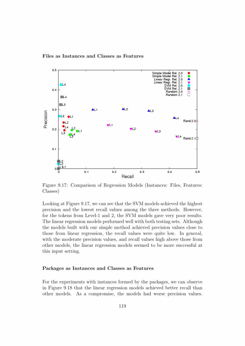
Files as Instances and Classes as Features
Figure 9.17: Comparison of Regression Models (Instances: Files, Features:Classes)
Looking at Figure 9.17, we can see that the SVM models achieved the highestprecision and the lowest recall values among the three methods. However,for the tokens from Level-1 and 2, the SVM models gave very poor results.The linear regression models performed well with both testing sets. Althoughthe models built with our simple method achieved precision values close tothose from linear regression, the recall values were quite low. In general,with the moderate precision values, and recall values high above those fromother models, the linear regression models seemed to be more successful atthis input setting.
Packages as Instances and Classes as Features
For the experiments with instances formed by the packages, we can observein Figure 9.18 that the linear regression models achieved better recall thanother models. As a compromise, the models had worse precision values.
119

Figure 9.18: Comparison of Regression Models (Instances: Packages, Fea-tures: Classes)
The low recall values from simple prediction models showed that the modelscovered a small percentage of failure-prone packages. Although we stated inSection 6.8 that the models with more precise results could be considered tobe better, when it comes to the risk class predictions; considering that thelinear regression models combined the relatively high precision values withthe higher recall rates, we believed that the results from the linear regressionmodels could be more useful.
Packages as Instances and Packages as Features
Whereas the results from the linear regression models in the last input settingstayed close to each other, and formed two clusters near the results from therandom classifier, the results from the simple models showed two differentstructures with the high precision and low recall values. Although the situ-ation in Figure 9.19 made the decision for the better model more difficult,we believed that, with the higher recall values, the linear regression modelscould be regarded as the better models in this setting.
120

Figure 9.19: Comparison of Regression Models (Instances: Packages, Fea-tures: Packages)
9.5 Usage Relations: General or Detailed?
As we have mentioned in Section 7.2, the import statements examined bySchroter et al. [47] gave an overview of the usage relations between compo-nents, whereas the tokens inspected in the second of our study provided moredetailed information about these relations. By applying the techniques de-scribed in Schroter et al.’s work, we aimed to see whether a detailed analysisof the usage relations would bring better predictions.
The linear regression and SVM models were also used Schroter et al., andthe results from our models showed similarities with those from Schroteret al.’s study. The authors achieved the best precision and recall valuesin the experiments where instances and attributes were collected under thepackages, and this situation was also observed in our experiments. Unliketheir models which achieved precision values around 90% for the top-riskypackages, our models were 80-84% precise for the same portion of testingsets.
121

Although, the authors decided that the best results were obtained from theirSVM models, in our case, the SVM models built with the same parametersfailed to make proper classifications in three experiment settings, making acomparison of the models impossible in our case.
For the linear regression models, in the experiments with packages as at-tributes, our models seemed to achieve precision values better than thosefrom Schroter et al. At the last two experiment settings (see Section 9.4.3and 9.4.4), our linear regression models had 80% precision for the most riskyclasses, whereas the precision values for the corresponding models in Schroteret al.’s study were lower. However almost 80% recall from these models werealmost impossible for our models to achieve.
Except those from our linear regression in the first experiment setting, theSpearman correlation values from our models weren’t significantly high. Sim-ilarly, the correlation values observed in Schroter et al.’s work were also low.So, in both studies, the ranking of the components based on the predictedfailure counts didn’t seem to provide valuable information about which com-ponents to examine first.
The usage relations captured by the Level 4 tokens in our study would overlapmostly with the relations examined Schroter et al., when the usage relationswhich came to being due to the accesses to the static methods and variables,and also the relations which couldn’t tracked by import statements (sincethe ‘*’ wildcard was used) weren’t taken into consideration. Excluding theexperiments in the second input setup, where our linear regression modelsgave erroneous results, we have compared the results from our and Schroter etal.’s linear regression models. The models from both studies achieved similarresults at the finest granularity of inputs. Our models gave better resultswhen the instances were collected under the packages, whereas Schroter etal.’s models had the higher recall but lower recall values than our models inthe last input setting. We believe that the results complied with each otherand showed that, one could predict the failure-proneness of components witha certain degree of success by inspecting the complete set of usage relationsbetween components.
9.6 Conclusion
The results from the regression experiments showed that all of our modelsperformed in most experiments better than a random classification model in
122

terms of precision. The linear regression models achieved also better recallvalues in many cases. The final comparisons of our results with those fromSchroter et al. [47] in Section 9.4.5 also indicated that the examination ofdifferent types of usage relations would be worthy. In light of all these results,we believe that the usage relations determine how risky the components willbe.
Usage relations have effects on the failure-proneness of com-
ponents.
In our experiments, the linear regression models made relatively precise pre-dictions and covered more of the risky components than other models. Sur-prisingly, the simple prediction models had the highest precision values, butthey could detect only a small portion of the risky files. The SVM modelshad difficulties at making clear separations between the classes and classifiedmost of the components to be risky. Based on these results, the linear modelsseemed to give more accurate predictions and to be relatively more robust.
Linear regression models work better than other models forclassification purposes.
Similar to the models of Schroter et al., our regression models also gavethe best results at the broader granularity of instances. For the most riskypackages, our models were in eight of ten cases correct in their decisions.
Risky packages can be detected more accurately than riskyfiles. Classification gives best results for the packages whichare most failure-prone.
Although the models we have built had high precision or recall values thanthe random classifier, the rankings of the components had less correlationwith the original failure rankings. This situation showed that the modelscouldn’t give good hints about in which component the developers shouldstart spending the extra effort.
123

Regression models weren’t good at risk rankings.
The comparisons in Section 9.4.5 showed us that, even though no modeldominated all other models, the results from the linear regression and simpleprediction models built on Level 1 tokens in Figures 9.17, 9.18, and 9.19 werecomparably good. Based on our results, we believed that the predictive mod-els could be built using only the information about the inheritance relations,which means that the models can be used even at the early design stages.Fulfilling the only requirement of keeping the inheritance relations betweencomponents in a format similar to our data matrix, one can use our modelswhile designing the components, without having to wait for the whole projectto finish to get the complete source code and to extract the Level 1 tokens.
Regression models can be also built on only inheritance rela-tions, which are defined very early in the project.
124

Chapter 10
Conclusion and Future Work
10.1 Conclusion
In this study, we tried to guide the managers and developers by predictingwhich parts of a software system may cause more problems than the others.In order to achieve this, we used statistical methods, and the data from theproject code and the software repositories.
The classification models built on the data from inheritance, method call,and variable tokens had successful outcomes, and provided support for ourhypothesis that there is a relation between specific code structures and post-release failures. The results from these models also indicated that usage re-lations between components may affect the failure-proneness of components.
When we took the design of the system as an evolving process and consid-ered the usage relations between components in a progressive manner; eventhough the failure counts predicted by our regression models didn’t provideuseful rankings in most cases, the accuracy of these models at different in-put granularities were promising. Our results complied with those from anearlier, similar study [47] and showed that it would be possible to accuratelydetect failure-prone packages, especially the ones that are most-risky.
Based on the results from regression models, we can say that even know-ing which classes or interfaces are used in a component may be sufficient topredict the failure-proneness of that component with a considerable preci-sion. This relation between inherited classes or interfaces, and the riskiness
125

indicates that, the difficulties at understanding and building a componentoriginate at the base components upon which new functionality is built. Thedevelopers should be sure that they understand the general properties of thesystem before they start specializing.
Getting the risk values for the components after determining the inheritancerelations may help the developers to be more careful about risky components,starting from the early phases of a project. With the necessary preventivemeasures against defects and failures taken early in the development process,the overall system reliability and quality can be improved significantly.
10.2 Future Work
Although this study has provided support for the existence of some importantrelations between the system design, program code, and failure-proneness ofsystem components, we believe that more interesting results are yet to come.We believe that the following issues could be the initial steps where we couldimprove our studies:
Other Statistical Methods The researchers have used different statisticalmethods to make predictions about failure-proneness of components ordefect densities in systems. Although we have used three of the com-monly used methods, we’d also like to test whether models of differenttechniques could perform better than the current ones.
Majority Vote In our study, we have collected the results from differentmodels and compared them against each other, trying to find a bestmethod. However, it could be also possible to combine the results fromall techniques to make a final decision. In that case, one may declarea component as risky depending on the decision which is suggested bythe majority of the used methods. Although this may be difficult forlarge projects (one has to build as many prediction models as statisticalmethods, which is very time-consuming with large inputs), it may bean option for small projects. With parallel programming approaches,such a computation may also be feasible for larger projects.
Design Time Metrics Showing that inheritance relations or the usage re-lations which are mainly defined in the design phase of the developmentbrings more questions about the effects of design on failures and systemquality. In order to answer these questions, further design metrics likedepth of inheritance could be examined.
126

Tool Support In this study, we have used small data processing programsto collect the information about programming structures and R-scriptsto build the statistical models and evaluate the results. We believe thatan automated tool that performs some of the steps described in ourstudy (collecting the information about failures and changes made toa system would probably be done by some other programs separately),and presents the predicted risk classes and risk values to the managersand developers would be definitely more useful.
Including Component Size in Input One can argue that larger sourcefiles or packages contain more tokens than smaller ones. Althoughthis is an acceptable argument, since we didn’t include any metricsin our models, the effects of code size wasn’t considered in our modelbuilding process. During this study, we believed that our models maycompensate for the effects of code size on predictions. However, infuture studies, we would like to investigate this issue by introducingthe size metric into our models. As an initial solution to the problem,we think that the tokens counts for the components can be normalizedwith a factor of LOC metric (i.e.log(LOC)).
Examining Other Projects Although we have inspected the Eclipse pro-ject, a large project built by professional developers, in our study, itwill be definitely useful to test the validity of our techniques on someother projects. The main problem in this case may be the collectionof the data about the problem reports and modifications made to asystem. With the improvements in software repositories which are infavor of the analyses such as ours, it will be easier to conduct suchstudies in the future.
Risk Propagation The success of our simple prediction models in the re-gression experiments not only validated our approach of estimatingriskiness but also brought some questions. While computing the riskvalues of testing instances as the average of the risk values of the at-tributes in those instances, riskiness was considered as a property thatpasses from one component to another, as a result of a usage relation.The success of the models of inheritance relations also provided sup-port in this direction. May it be the case that risk simply propagates?Can we find better prediction models based on this idea?
We believe that the answers to these and similar questions will help us tounderstand the causes behind the errors in software projects, and to developbetter and more reliable software systems.
127

Appendix A
Regression ExperimentsResults
128

A.1 Linear Regression Models
Release 2.0
Level Pct. Prec. Recall Spear. Level Pct. Prec. Recall Spear.
L1
100% 0.2989 0.1242 0.5221
5% 0.3059 -0.0135
10% 0.2706 -0.0080
15% 0.2088 -0.0470
20% 0.1580 -0.0556
L2
100% 0.3018 0.2334 0.4465
F2
100% 0.3060 0.3012 0.4722
5% 0.3421 0.0148 5% 0.3509 -0.0936
10% 0.3179 0.1075 10% 0.3223 -0.0662
15% 0.2993 0.0698 15% 0.3065 0.0414
20% 0.2574 -0.0515 20% 0.2608 -0.1045
L3
100% 0.2932 0.3261 0.2754
F3
100% 0.3092 0.2870 0.4913
5% 0.3742 0.0449 5% 0.3643 0.0030
10% 0.3490 0.0843 10% 0.3431 0.1061
15% 0.3318 0.0901 15% 0.3271 0.0486
20% 0.3137 0.1424 20% 0.3078 -0.0097
L4
100% 0.2571 0.4177 0.2955
F4
100% 0.2879 0.3413 0.4979
5% 0.4140 0.0268 5% 0.4243 -0.0054
10% 0.3623 0.0520 10% 0.3728 0.0182
15% 0.3298 0.0803 15% 0.3387 0.0623
20% 0.3075 0.1059 20% 0.3106 -0.0281
Table A.1: Results of Linear Regression Models - Release 2.0 Testing Data -Instances: Files, Features: Classes
129

Release 2.1
Level Pct. Prec. Recall Spear. Level Pct. Prec. Recall Spear.
L1
100% 0.2218 0.1790 0.5679
5% 0.2630 -0.0587
10% 0.2169 0.0074
15% 0.1739 0.3599
20% 0.1371 0.2012
L2
100% 0.2026 0.2618 0.3240
F2
100% 0.1968 0.3145 0.5731
5% 0.2440 0.0133 5% 0.2511 -0.0863
10% 0.2260 0.0646 10% 0.2286 -0.0836
15% 0.2115 0.2161 15% 0.2124 0.2333
20% 0.1852 0.1364 20% 0.1801 0.2227
L3
100% 0.1893 0.3514 0.2787
F3
100% 0.2027 0.3239 0.3024
5% 0.2611 0.0575 5% 0.2613 0.0261
10% 0.2351 0.1396 10% 0.2355 0.1029
15% 0.2184 0.1558 15% 0.2250 0.2107
20% 0.2061 0.1168 20% 0.2113 0.1098
L4
100% 0.1641 0.4266 0.2833
F4
100% 0.1871 0.3628 0.3302
5% 0.2387 0.0272 5% 0.2625 0.0123
10% 0.2176 0.1287 10% 0.2426 0.0714
15% 0.2036 0.1055 15% 0.2231 0.1854
20% 0.1918 0.0832 20% 0.2047 0.1057
Table A.2: Results of Linear Regression Models - Release 2.1 Testing Data -Instances: Files, Features: Classes
130

Release 2.0
Level Pct. Prec. Recall Spear. Level Pct. Prec. Recall Spear.
L1
100% 0.2663 0.8594 0.4553
5% 0.4184 0.0585
10% 0.3671 0.1816
15% 0.3298 -0.0129
20% 0.3066 -0.0409
L2
100% 0.2554 0.8919 0.2664
F2
100% 0.2581 0.8899 0.4762
5% 0.4146 0.0536 5% 0.4202 0.0324
10% 0.3793 0.1684 10% 0.3843 0.1791
15% 0.3574 0.0288 15% 0.3602 0.0603
20% 0.3335 0.1151 20% 0.3419 -0.0106
L3
100% 0.2378 0.8785 0.2155
F3
100% 0.2430 0.8716 0.2564
5% 0.4265 0.0247 5% 0.4261 0.0263
10% 0.3808 0.1240 10% 0.3764 0.1514
15% 0.3499 0.0607 15% 0.3499 0.0200
20% 0.3327 0.1275 20% 0.3314 0.1388
L4
100% 0.2323 0.8257 0.2442
F4
100% 0.2349 0.8301 0.2951
5% 0.4395 0.0238 5% 0.4455 0.0374
10% 0.4030 0.1007 10% 0.4048 0.1069
15% 0.3765 0.0586 15% 0.3767 0.0213
20% 0.3540 0.1263 20% 0.3607 0.1509
Table A.3: Results of Linear Regression Models - Release 2.0 Testing Data -Instances: Files, Features: Packages
131

Release 2.1
Level Pct. Prec. Recall Spear. Level Pct. Prec. Recall Spear.
L1
100% 0.1606 0.8600 0.3335
5% 0.2826 0.0901
10% 0.2477 0.1180
15% 0.2244 0.2722
20% 0.2101 0.0965
L2
100% 0.1558 0.8879 0.2696
F2
100% 0.1536 0.8826 0.3170
5% 0.2875 0.0808 5% 0.2875 0.0701
10% 0.2511 0.1156 10% 0.2557 0.0962
15% 0.2364 0.1743 15% 0.2328 0.2326
20% 0.2230 0.1169 20% 0.2179 0.1328
L3
100% 0.1464 0.8829 0.2727
F3
100% 0.1457 0.8760 0.2858
5% 0.2799 0.0231 5% 0.2778 0.0131
10% 0.2565 0.1453 10% 0.2521 0.1641
15% 0.2399 0.1559 15% 0.2367 0.1746
20% 0.2277 0.1546 20% 0.2218 0.1141
L4
100% 0.1446 0.8404 0.2839
F4
100% 0.1437 0.8391 0.3019
5% 0.2699 -0.0089 5% 0.2667 -0.0201
10% 0.2539 0.1489 10% 0.2510 0.1686
15% 0.2434 0.1790 15% 0.2383 0.1825
20% 0.2322 0.1544 20% 0.2273 0.1322
Table A.4: Results of Linear Regression Models - Release 2.1 Testing Data -Instances: Files, Features: Packages
132

Release 2.0
Level Pct. Prec. Recall Spear. Level Pct. Prec. Recall Spear.
L1
100% 0.6526 0.5811 0.0179
5% 0.7975 -0.0656
10% 0.7822 -0.0377
15% 0.7710 0.0051
20% 0.7601 0.0131
L2
100% 0.6616 0.5414 0.0835
F2
100% 0.6580 0.5682 0.0111
5% 0.8107 -0.0300 5% 0.8198 0.0655
10% 0.8011 0.0530 10% 0.7912 0.0158
15% 0.7994 -0.0032 15% 0.7774 0.0034
20% 0.7880 -0.0086 20% 0.7560 0.0529
L3
100% 0.6749 0.5205 0.0548
F3
100% 0.6607 0.5499 0.0027
5% 0.7991 0.0636 5% 0.8407 -0.0524
10% 0.8064 -0.0076 10% 0.8059 -0.0276
15% 0.7917 -0.0127 15% 0.7684 -0.0389
20% 0.7818 0.0247 20% 0.7508 -0.0258
L4
100% 0.6854 0.4833 0.0443
F4
100% 0.6659 0.5182 0.0054
5% 0.7884 -0.0901 5% 0.8143 -0.0443
10% 0.7452 -0.0660 10% 0.7872 0.0015
15% 0.7365 -0.0435 15% 0.7689 0.0053
20% 0.7198 -0.0305 20% 0.7635 -0.0003
Table A.5: Results of Linear Regression Models - Release 2.0 Testing Data -Instances: Packages, Features: Classes
133

Release 2.1
Level Pct. Prec. Recall Spear. Level Pct. Prec. Recall Spear.
L1
100% 0.5859 0.5939 0.0670
5% 0.7718 -0.0275
10% 0.7381 0.0949
15% 0.7023 0.0934
20% 0.6793 0.0694
L2
100% 0.6083 0.5543 0.1009
F2
100% 0.5785 0.5661 0.0162
5% 0.7731 -0.0353 5% 0.7440 -0.0019
10% 0.7416 0.0060 10% 0.7190 0.0461
15% 0.7205 -0.0030 15% 0.6862 0.0686
20% 0.7115 -0.0102 20% 0.6697 0.0330
L3
100% 0.5916 0.5240 0.0806
F3
100% 0.5701 0.5509 0.0365
5% 0.7694 0.0063 5% 0.7625 -0.0472
10% 0.7505 0.0499 10% 0.7177 0.0175
15% 0.7312 0.0388 15% 0.7049 0.0504
20% 0.7179 0.0211 20% 0.6743 0.0163
L4
100% 0.6052 0.4835 0.0752
F4
100% 0.5890 0.5238 0.0480
5% 0.7765 0.0107 5% 0.7664 -0.0389
10% 0.7270 0.0127 10% 0.7284 -0.0339
15% 0.7010 -0.0119 15% 0.7160 -0.0103
20% 0.6804 0.0210 20% 0.6917 -0.0049
Table A.6: Results of Linear Regression Models - Release 2.1 Testing Data -Instances: Packages, Features: Classes
134
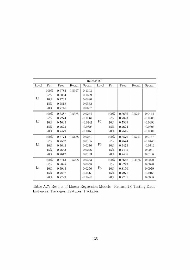
Release 2.0
Level Pct. Prec. Recall Spear. Level Pct. Prec. Recall Spear.
L1
100% 0.6782 0.5397 0.1303
5% 0.8054 0.1399
10% 0.7763 0.0890
15% 0.7818 0.0532
20% 0.7748 0.0637
L2
100% 0.6387 0.5385 0.0254
F2
100% 0.6636 0.5214 0.0444
5% 0.7274 -0.0064 5% 0.7823 -0.0906
10% 0.7645 -0.0441 10% 0.7599 -0.0693
15% 0.7623 -0.0326 15% 0.7624 -0.0606
20% 0.7479 -0.0158 20% 0.7515 -0.0304
L3
100% 0.6774 0.5188 0.0261
F3
100% 0.6570 0.5221 0.0157
5% 0.7552 0.0105 5% 0.7574 -0.0446
10% 0.7642 0.0276 10% 0.7473 -0.0712
15% 0.7653 0.0246 15% 0.7435 0.0031
20% 0.7612 0.0133 20% 0.7406 0.0166
L4
100% 0.6713 0.5208 0.0363
F4
100% 0.6648 0.4975 0.0220
5% 0.8028 0.0858 5% 0.8273 0.0020
10% 0.7943 0.0256 10% 0.8150 0.0079
15% 0.7837 -0.0260 15% 0.7971 -0.0163
20% 0.7729 -0.0244 20% 0.7731 0.0008
Table A.7: Results of Linear Regression Models - Release 2.0 Testing Data -Instances: Packages, Features: Packages
135

Release 2.1
Level Pct. Prec. Recall Spear. Level Pct. Prec. Recall Spear.
L1
100% 0.4634 0.5585 0.3210
5% 0.7036 0.0059
10% 0.6803 0.0229
15% 0.6503 0.0719
20% 0.6218 0.0647
L2
100% 0.4268 0.5381 0.2734
F2
100% 0.4615 0.5357 0.2996
5% 0.7079 0.0246 5% 0.7274 0.0090
10% 0.6859 0.0069 10% 0.6922 -0.0185
15% 0.6534 0.0171 15% 0.6552 -0.0056
20% 0.6173 0.0401 20% 0.6211 0.0200
L3
100% 0.4626 0.5232 0.2525
F3
100% 0.4456 0.5350 0.2480
5% 0.7113 0.0594 5% 0.6911 -0.0204
10% 0.6844 0.0591 10% 0.6783 0.0187
15% 0.6455 0.0585 15% 0.6440 0.0432
20% 0.6269 0.0793 20% 0.6098 0.0474
L4
100% 0.4505 0.5225 0.2409
F4
100% 0.4318 0.4851 0.2129
5% 0.6485 -0.0226 5% 0.6679 -0.0427
10% 0.6608 0.0227 10% 0.6532 -0.0152
15% 0.6312 0.0155 15% 0.6231 0.0093
20% 0.6194 0.0298 20% 0.5983 0.0019
Table A.8: Results of Linear Regression Models - Release 2.1 Testing Data -Instances: Packages, Features: Packages
136

A.2 Support Vector Machines Models
Release 2.0
Level Pct. Prec. Recall Spear. Level Pct. Prec. Recall Spear.
L1
100% 0.0000 0.0000 0.5468
5% 0.0000 0.0786
10% 0.0000 0.1953
15% 0.0000 0.0191
20% 0.0000 -0.0704
L2
100% 0.0256 0.0000 0.2164
F2
100% 0.0000 0.0000 0.2522
5% 0.0001 0.1297 5% 0.0000 0.0981
10% 0.0001 0.2234 10% 0.0000 0.2369
15% 0.0000 0.0812 15% 0.0000 0.0464
20% 0.0000 0.1523 20% 0.0000 0.1521
L3
100% 0.2669 0.0042 0.2136
F3
100% 0.3131 0.0049 0.2152
5% 0.0189 0.1256 5% 0.0228 0.1355
10% 0.0094 0.1423 10% 0.0114 0.1344
15% 0.0063 0.1390 15% 0.0076 0.1318
20% 0.0047 0.1505 20% 0.0057 0.1540
L4
100% 0.4263 0.0089 0.2116
F4
100% 0.4735 0.0106 0.2088
5% 0.0408 0.1316 5% 0.0493 0.1336
10% 0.0204 0.1456 10% 0.0246 0.1464
15% 0.0136 0.1649 15% 0.0164 0.1659
20% 0.0102 0.1692 20% 0.0123 0.1665
Table A.9: Results of Support Vector Machines Models - Release 2.0 TestingData - Instances: Files, Features: Classes
137

Release 2.1
Level Pct. Prec. Recall Spear. Level Pct. Prec. Recall Spear.
L1
100% 0.0000 0.0000 0.3721
5% 0.0000 -0.0121
10% 0.0000 0.0888
15% 0.0000 0.3251
20% 0.0000 0.1554
L2
100% 0.0385 0.0001 0.2777
F2
100% 0.0513 0.0001 0.2927
5% 0.0002 0.0773 5% 0.0002 0.0862
10% 0.0001 0.1499 10% 0.0001 0.1580
15% 0.0001 0.2036 15% 0.0001 0.2338
20% 0.0001 0.1198 20% 0.0001 0.1104
L3
100% 0.3250 0.0082 0.2937
F3
100% 0.3336 0.0083 0.2942
5% 0.0241 0.0794 5% 0.0243 0.0693
10% 0.0121 0.1712 10% 0.0121 0.1676
15% 0.0080 0.1881 15% 0.0081 0.1884
20% 0.0060 0.1384 20% 0.0061 0.1290
L4
100% 0.3638 0.0125 0.2962
F4
100% 0.4004 0.0146 0.3002
5% 0.0354 0.0527 5% 0.0413 0.0601
10% 0.0177 0.1664 10% 0.0206 0.1615
15% 0.0118 0.1910 15% 0.0138 0.1878
20% 0.0088 0.1266 20% 0.0103 0.1262
Table A.10: Results of Support Vector Machines Models - Release 2.1 TestingData - Instances: Files, Features: Classes
138

Release 2.0
Level Pct. Prec. Recall Spear. Level Pct. Prec. Recall Spear.
L1
100% 0.2657 0.9946 0.4271
5% 0.4360 0.0086
10% 0.3881 0.1318
15% 0.3553 0.0771
20% 0.3391 0.0252
L2
100% 0.2602 0.9936 0.2232
F2
100% 0.2637 0.9932 0.2323
5% 0.4574 0.0545 5% 0.4701 0.0714
10% 0.4112 0.1345 10% 0.4204 0.1491
15% 0.3915 0.0877 15% 0.4022 0.0900
20% 0.3723 0.1436 20% 0.3823 0.1448
L3
100% 0.2434 0.9919 0.2238
F3
100% 0.2485 0.9917 0.2292
5% 0.4819 0.1189 5% 0.4946 0.1375
10% 0.4277 0.0971 10% 0.4419 0.0944
15% 0.4028 0.1466 15% 0.4143 0.1722
20% 0.3805 0.1426 20% 0.3907 0.1480
L4
100% 0.2436 0.9929 0.2263
F4
100% 0.2457 0.9954 0.2271
5% 0.5149 0.0869 5% 0.5307 0.0983
10% 0.4431 0.0818 10% 0.4504 0.0799
15% 0.4064 0.1558 15% 0.4115 0.1579
20% 0.3838 0.1687 20% 0.3872 0.1723
Table A.11: Results of Support Vector Machines Models - Release 2.0 TestingData - Instances: Files, Features: Packages
139

Release 2.1
Level Pct. Prec. Recall Spear. Level Pct. Prec. Recall Spear.
L1
100% 0.1596 0.9939 0.3554
5% 0.2720 0.0268
10% 0.2365 0.1672
15% 0.2109 0.2266
20% 0.1990 0.1251
L2
100% 0.1598 0.9951 0.2879
F2
100% 0.1585 0.9940 0.2993
5% 0.2980 0.0820 5% 0.3029 0.0879
10% 0.2620 0.1578 10% 0.2657 0.1589
15% 0.2347 0.1705 15% 0.2394 0.1858
20% 0.2187 0.1235 20% 0.2227 0.1010
L3
100% 0.1506 0.9957 0.3098
F3
100% 0.1501 0.9959 0.3099
5% 0.2662 0.1019 5% 0.2717 0.1025
10% 0.2379 0.1943 10% 0.2447 0.1985
15% 0.2228 0.1515 15% 0.2239 0.1623
20% 0.2096 0.1141 20% 0.2110 0.0845
L4
100% 0.1509 0.9953 0.3237
F4
100% 0.1507 0.9973 0.3241
5% 0.3206 0.0356 5% 0.3302 0.0314
10% 0.2576 0.1874 10% 0.2617 0.1928
15% 0.2298 0.1722 15% 0.2321 0.1778
20% 0.2054 0.0775 20% 0.2072 0.0729
Table A.12: Results of Support Vector Machines Models - Release 2.1 TestingData - Instances: Files, Features: Packages
140

Release 2.0
Level Pct. Prec. Recall Spear. Level Pct. Prec. Recall Spear.
L1
100% 0.6397 1.0000 0.3696
5% 0.7786 0.4843
10% 0.8226 0.3832
15% 0.8062 0.4492
20% 0.7833 0.5099
L2
100% 0.6587 1.0000 0.4060
F2
100% 0.6516 1.0000 0.3799
5% 0.7509 0.6689 5% 0.7469 0.6139
10% 0.7938 0.5357 10% 0.7904 0.5132
15% 0.7858 0.5049 15% 0.7851 0.5193
20% 0.7856 0.4994 20% 0.7783 0.5119
L3
100% 0.6751 1.0000 0.4030
F3
100% 0.6663 1.0000 0.4113
5% 0.7832 0.6736 5% 0.7340 0.6967
10% 0.7444 0.4640 10% 0.7375 0.4754
15% 0.7948 0.3885 15% 0.7888 0.4550
20% 0.8139 0.3876 20% 0.8043 0.4831
L4
100% 0.6751 1.0000 0.4157
F4
100% 0.6747 1.0000 0.4054
5% 0.8412 0.6811 5% 0.8364 0.6719
10% 0.8213 0.4398 10% 0.8124 0.4389
15% 0.8249 0.3092 15% 0.8230 0.3674
20% 0.8134 0.3558 20% 0.8050 0.4015
Table A.13: Results of Support Vector Machines Models - Release 2.0 TestingData - Instances: Packages, Features: Classes
141

Release 2.1
Level Pct. Prec. Recall Spear. Level Pct. Prec. Recall Spear.
L1
100% 0.5705 1.0000 0.3167
5% 0.7572 0.2880
10% 0.8017 0.4562
15% 0.7687 0.3141
20% 0.7477 0.2961
L2
100% 0.5988 1.0000 0.3387
F2
100% 0.5764 1.0000 0.3311
5% 0.7937 0.4540 5% 0.7907 0.4911
10% 0.8342 0.4157 10% 0.8313 0.5018
15% 0.7942 0.2758 15% 0.7838 0.3151
20% 0.7763 0.2829 20% 0.7597 0.2847
L3
100% 0.5950 1.0000 0.2904
F3
100% 0.5764 1.0000 0.2993
5% 0.8159 0.3245 5% 0.7756 0.4905
10% 0.7746 0.3772 10% 0.7543 0.4173
15% 0.7937 0.331 15% 0.7819 0.2821
20% 0.7696 0.2025 20% 0.7607 0.2378
L4
100% 0.5950 1.0000 0.2693
F4
100% 0.5921 1.0000 0.2618
5% 0.8437 0.3127 5% 0.8257 0.4261
10% 0.7789 0.3561 10% 0.7681 0.3796
15% 0.7717 0.3365 15% 0.7627 0.2950
20% 0.7671 0.1869 20% 0.7542 0.1965
Table A.14: Results of Support Vector Machines Models - Release 2.1 TestingData - Instances: Packages, Features: Classes
142

Release 2.0
Level Pct. Prec. Recall Spear. Level Pct. Prec. Recall Spear.
L1
100% 0.6396 0.9991 0.4199
5% 0.8629 0.4145
10% 0.8517 0.3789
15% 0.8323 0.4780
20% 0.8121 0.4994
L2
100% 0.6585 0.9991 0.4261
F2
100% 0.6514 0.9995 0.4294
5% 0.7809 0.3463 5% 0.7763 0.3546
10% 0.7529 0.4203 10% 0.7617 0.3819
15% 0.7694 0.4459 15% 0.7653 0.4528
20% 0.7985 0.4406 20% 0.7969 0.4679
L3
100% 0.6751 0.9992 0.3521
F3
100% 0.6663 0.9995 0.3593
5% 0.7930 0.0655 5% 0.7873 0.0621
10% 0.7867 0.1039 10% 0.7796 0.0595
15% 0.7633 0.1090 15% 0.7609 0.1416
20% 0.7903 0.1120 20% 0.7887 0.2004
L4
100% 0.6750 0.9993 0.2125
F4
100% 0.6745 0.9990 0.2087
5% 0.8271 0.0933 5% 0.8252 0.1044
10% 0.7967 -0.0029 10% 0.7898 0.0004
15% 0.8107 0.0063 15% 0.8088 0.0093
20% 0.7729 -0.0347 20% 0.7659 -0.0315
Table A.15: Results of Support Vector Machines Models - Release 2.0 TestingData - Instances: Packages, Features: Packages
143

Release 2.1
Level Pct. Prec. Recall Spear. Level Pct. Prec. Recall Spear.
L1
100% 0.4301 0.9994 0.2013
5% 0.8381 0.1938
10% 0.7817 0.0386
15% 0.7226 0.1181
20% 0.6752 0.1412
L2
100% 0.4449 0.9991 0.2028
F2
100% 0.4412 0.9998 0.2122
5% 0.8107 -0.0983 5% 0.8072 0.0366
10% 0.7750 -0.0269 10% 0.7745 0.0544
15% 0.7562 0.0132 15% 0.7581 0.0670
20% 0.7211 0.0293 20% 0.7254 0.0534
L3
100% 0.4502 0.9991 0.1794
F3
100% 0.4464 0.9993 0.1752
5% 0.5900 -0.1807 5% 0.5694 -0.0872
10% 0.6544 -0.1729 10% 0.6486 -0.1285
15% 0.7093 -0.0340 15% 0.7104 -0.0349
20% 0.7134 -0.0616 20% 0.7163 -0.0150
L4
100% 0.4503 0.9995 0.2002
F4
100% 0.4465 0.9993 0.1897
5% 0.5662 -0.0740 5% 0.5609 -0.0098
10% 0.4579 -0.1834 10% 0.4576 -0.1457
15% 0.4824 -0.1490 15% 0.4792 -0.1676
20% 0.4995 -0.1963 20% 0.4938 -0.2106
Table A.16: Results of Support Vector Machines Models - Release 2.1 TestingData - Instances: Packages, Features: Packages
144

A.3 Simple Prediction Models
Release 2.0
Level Pct. Prec. Recall Spear. Level Pct. Prec. Recall Spear.
L1
100% 0.2638 0.0370 0.7332
5% 0.1786 0.1044
10% 0.0973 0.2177
15% 0.0648 0.0116
20% 0.0486 -0.0571
L2
100% 0.2346 0.0190 0.1774
F2
100% 0.2521 0.0227 0.4657
5% 0.0970 0.0632 20% 0.1192 0.1093
10% 0.0484 0.2156 20% 0.0595 0.3986
15% 0.0322 0.0529 20% 0.0396 -0.0592
20% 0.0242 0.1246 20% 0.0297 0.1561
L3
100% 0.1957 0.0217 0.1870
F3
100% 0.2054 0.0315 0.1902
20% 0.1021 0.0317 20% 0.1426 -0.0161
20% 0.0526 0.0310 20% 0.0787 0.0926
20% 0.0350 0.0087 20% 0.0524 0.0429
20% 0.0263 0.0784 20% 0.0393 0.1168
L4
100% 0.2155 0.0182 0.1843
F4
100% 0.2192 0.0248 0.1846
20% 0.0897 -0.0025 20% 0.1203 -0.0486
20% 0.0448 0.0355 20% 0.0618 0.0363
20% 0.0298 -0.0026 20% 0.0412 0.0345
20% 0.0224 0.0838 20% 0.0309 0.1307
Table A.17: Results of Simple Prediction Models - Release 2.0 Testing Data- Instances: Files, Features: Classes
145
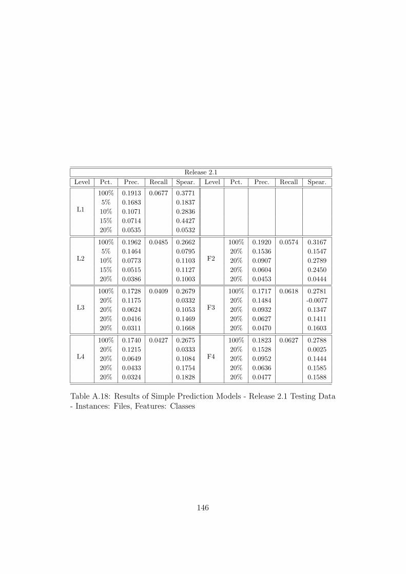
Release 2.1
Level Pct. Prec. Recall Spear. Level Pct. Prec. Recall Spear.
L1
100% 0.1913 0.0677 0.3771
5% 0.1683 0.1837
10% 0.1071 0.2836
15% 0.0714 0.4427
20% 0.0535 0.0532
L2
100% 0.1962 0.0485 0.2662
F2
100% 0.1920 0.0574 0.3167
5% 0.1464 0.0795 20% 0.1536 0.1547
10% 0.0773 0.1103 20% 0.0907 0.2789
15% 0.0515 0.1127 20% 0.0604 0.2450
20% 0.0386 0.1003 20% 0.0453 0.0444
L3
100% 0.1728 0.0409 0.2679
F3
100% 0.1717 0.0618 0.2781
20% 0.1175 0.0332 20% 0.1484 -0.0077
20% 0.0624 0.1053 20% 0.0932 0.1347
20% 0.0416 0.1469 20% 0.0627 0.1411
20% 0.0311 0.1668 20% 0.0470 0.1603
L4
100% 0.1740 0.0427 0.2675
F4
100% 0.1823 0.0627 0.2788
20% 0.1215 0.0333 20% 0.1528 0.0025
20% 0.0649 0.1084 20% 0.0952 0.1444
20% 0.0433 0.1754 20% 0.0636 0.1585
20% 0.0324 0.1828 20% 0.0477 0.1588
Table A.18: Results of Simple Prediction Models - Release 2.1 Testing Data- Instances: Files, Features: Classes
146

Release 2.0
Level Pct. Prec. Recall Spear. Level Pct. Prec. Recall Spear.
L1
100% 0.2786 0.0465 0.2483
5% 0.1971 0.0764
10% 0.1186 0.3287
15% 0.0824 -0.0686
20% 0.0623 0.1984
L2
100% 0.2477 0.0232 0.1550
F2
100% 0.2621 0.0308 0.1867
5% 0.1194 0.0590 5% 0.1461 0.0161
10% 0.0616 0.1273 10% 0.0815 0.2391
15% 0.0410 0.0303 15% 0.0551 0.0281
20% 0.0307 0.0960 20% 0.0413 0.1643
L3
100% 0.2104 0.0124 0.1868
F3
100% 0.2452 0.0270 0.1643
5% 0.0577 0.0286 5% 0.1305 0.0403
10% 0.0288 0.0470 10% 0.0667 0.0499
15% 0.0192 -0.0014 15% 0.0445 -0.0023
20% 0.0144 0.0748 20% 0.0333 0.0976
L4
100% 0.1763 0.0134 0.1743
F4
100% 0.2665 0.0293 0.1752
5% 0.0626 -0.0002 5% 0.1423 -0.0319
10% 0.0313 0.0529 10% 0.0716 0.0388
15% 0.0208 -0.0103 15% 0.0477 0.0081
20% 0.0156 0.0839 20% 0.0358 0.1165
Table A.19: Results of Simple Prediction Models - Release 2.0 Testing Data- Instances: Files, Features: Packages
147

Release 2.1
Level Pct. Prec. Recall Spear. Level Pct. Prec. Recall Spear.
L1
100% 0.1963 0.0512 0.2848
5% 0.1244 0.1573
10% 0.0769 0.2035
15% 0.0548 0.1757
20% 0.0413 0.0595
L2
100% 0.1800 0.0233 0.2547
F2
100% 0.1875 0.0363 0.2637
5% 0.0730 0.1082 5% 0.0980 0.1353
10% 0.0382 0.0974 10% 0.0580 0.1453
15% 0.0254 0.1143 15% 0.0393 0.1305
20% 0.0191 0.1562 20% 0.0295 0.1119
L3
100% 0.1531 0.0106 0.2615
F3
100% 0.1653 0.0265 0.2643
5% 0.0315 0.0680 5% 0.0772 0.0440
10% 0.0157 0.0922 10% 0.0402 0.1001
15% 0.0105 0.1625 15% 0.0268 0.1565
20% 0.0078 0.2132 20% 0.0201 0.2152
L4
100% 0.1007 0.0090 0.2500
F4
100% 0.1458 0.0257 0.2533
5% 0.0264 0.0550 5% 0.0761 0.0223
10% 0.0132 0.1048 10% 0.0383 0.1169
15% 0.0088 0.1771 15% 0.0255 0.1748
20% 0.0066 0.2273 20% 0.0191 0.2107
Table A.20: Results of Simple Prediction Models - Release 2.1 Testing Data- Instances: Files, Features: Packages
148

Release 2.0
Level Pct. Prec. Recall Spear. Level Pct. Prec. Recall Spear.
L1
100% 0.7582 0.3108 0.2599
5% 0.8125 -0.1324
10% 0.7710 -0.0418
15% 0.7371 -0.1035
20% 0.7212 -0.0473
L2
100% 0.7746 0.2446 0.2372
F2
100% 0.7724 0.2546 0.2317
5% 0.7707 0.2880 5% 0.8159 0.3367
10% 0.7572 0.1188 10% 0.7498 0.1324
15% 0.7371 0.0677 15% 0.7312 0.0641
20% 0.6907 0.0777 20% 0.7003 0.0633
L3
100% 0.7756 0.2201 0.2082
F3
100% 0.7674 0.2917 0.1880
5% 0.7783 0.4080 5% 0.7820 0.3800
10% 0.7596 0.0875 10% 0.7759 0.0350
15% 0.7055 0.0062 15% 0.7625 0.0196
20% 0.6406 -0.0046 20% 0.7362 0.0133
L4
100% 0.8096 0.1408 0.2140
F4
100% 0.7979 0.1846 0.1819
5% 0.8283 0.4483 5% 0.8210 0.4586
10% 0.7133 0.1181 10% 0.7699 0.1064
15% 0.5927 0.0376 15% 0.6850 0.0321
20% 0.4662 -0.026 20% 0.5889 -0.0340
Table A.21: Results of Simple Prediction Models - Release 2.0 Testing Data- Instances: Packages, Features: Classes
149
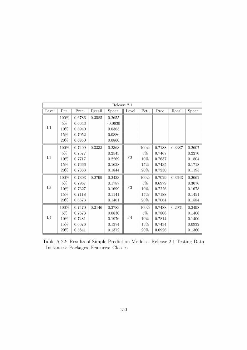
Release 2.1
Level Pct. Prec. Recall Spear. Level Pct. Prec. Recall Spear.
L1
100% 0.6786 0.3585 0.2655
5% 0.6643 -0.0630
10% 0.6940 0.0363
15% 0.7052 0.0886
20% 0.6850 0.0860
L2
100% 0.7409 0.3333 0.2363
F2
100% 0.7188 0.3387 0.2607
5% 0.7577 0.2543 5% 0.7467 0.2270
10% 0.7717 0.2269 10% 0.7637 0.1804
15% 0.7666 0.1638 15% 0.7435 0.1718
20% 0.7333 0.1844 20% 0.7230 0.1195
L3
100% 0.7303 0.2799 0.2433
F3
100% 0.7029 0.3643 0.2062
5% 0.7967 0.1787 5% 0.6979 0.3076
10% 0.7327 0.1699 10% 0.7226 0.1678
15% 0.7118 0.1141 15% 0.7188 0.1451
20% 0.6573 0.1461 20% 0.7064 0.1584
L4
100% 0.7470 0.2146 0.2783
F4
100% 0.7488 0.2931 0.2498
5% 0.7673 0.0830 5% 0.7806 0.1406
10% 0.7481 0.1976 10% 0.7814 0.1400
15% 0.6676 0.1374 15% 0.7434 0.0932
20% 0.5841 0.1372 20% 0.6926 0.1360
Table A.22: Results of Simple Prediction Models - Release 2.1 Testing Data- Instances: Packages, Features: Classes
150

Release 2.0
Level Pct. Prec. Recall Spear. Level Pct. Prec. Recall Spear.
L1
100% 0.7661 0.2169 0.1714
5% 0.7533 -0.0578
10% 0.7275 -0.1124
15% 0.6748 -0.0950
20% 0.5930 -0.0233
L2
100% 0.7706 0.1225 0.1842
F2
100% 0.7464 0.1509 0.1490
5% 0.7681 0.1613 5% 0.7527 0.1504
10% 0.6298 0.0188 10% 0.6436 -0.0135
15% 0.4932 -0.0330 15% 0.5411 -0.0323
20% 0.3947 -0.0418 20% 0.4476 -0.0125
L3
100% 0.7953 0.0825 0.1628
F3
100% 0.7992 0.1253 0.1131
5% 0.6760 0.2753 5% 0.7444 0.2758
10% 0.5085 0.0683 10% 0.6015 0.0161
15% 0.3764 0.0361 15% 0.4978 0.2824
20% 0.2811 -0.0170 20% 0.4049 -0.0216
L4
100% 0.8359 0.0546 0.2121
F4
100% 0.8255 0.0803 0.1824
5% 0.6419 0.2714 5% 0.7232 0.3386
10% 0.3731 0.0089 10% 0.5223 -0.0481
15% 0.2475 -0.0529 15% 0.3633 -0.0586
20% 0.1846 -0.0228 20% 0.2709 -0.0159
Table A.23: Results of Simple Prediction Models - Release 2.0 Testing Data- Instances: Packages, Features: Packages
151
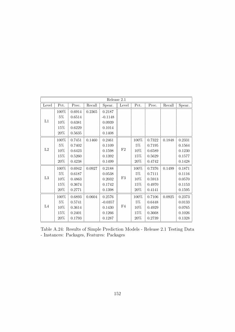
Release 2.1
Level Pct. Prec. Recall Spear. Level Pct. Prec. Recall Spear.
L1
100% 0.6914 0.2365 0.2187
5% 0.6514 -0.1148
10% 0.6381 0.0939
15% 0.6229 0.1014
20% 0.5635 0.1408
L2
100% 0.7451 0.1460 0.2461
F2
100% 0.7322 0.1848 0.2331
5% 0.7402 0.1109 5% 0.7195 0.1564
10% 0.6423 0.1598 10% 0.6589 0.1230
15% 0.5260 0.1392 15% 0.5629 0.1577
20% 0.4238 0.1499 20% 0.4742 0.1428
L3
100% 0.6942 0.0927 0.2188
F3
100% 0.7376 0.1499 0.1871
5% 0.6187 0.0538 5% 0.7111 0.1116
10% 0.4863 0.2032 10% 0.5913 0.0570
15% 0.3674 0.1742 15% 0.4970 0.1153
20% 0.2771 0.1398 20% 0.4141 0.1595
L4
100% 0.6893 0.0604 0.2576
F4
100% 0.7106 0.0925 0.2373
5% 0.5741 -0.0357 5% 0.6448 0.0133
10% 0.3614 0.1430 10% 0.4929 0.0765
15% 0.2401 0.1266 15% 0.3668 0.1026
20% 0.1793 0.1287 20% 0.2739 0.1328
Table A.24: Results of Simple Prediction Models - Release 2.1 Testing Data- Instances: Packages, Features: Packages
152

Bibliography
[1] A. Andrews and C. Stringfellow. Quantitative Analysis of DevelopmentDefects to Guide Testing: A Case Study. Software Quality Journal,9(3):195–214, 2001.
[2] ASM Java Bytecode Manipulation Framework. Available from:http://asm.objectweb.org/index.html (last visited: 22 October 2006).
[3] AST View Plugin for Eclipse. Available from: http://www.eclipse.org/jdt/ui/astview/index.php (last visited: 22 October 2006).
[4] S. Bibi, G. Tsoumakas, I. Stamelos, and I. Vlahavas. Software DefectPrediction Using Regression via Classification. In Proceedings of theFourth ACS/IEEE International Conference on Computer Systems andApplications, pages 330–336, Dubai/Sharjah, UAE, 2006. IEEE Com-puter Society Press.
[5] Binkley, A. B. and Schach, S. R. Metrics for Predicting Run-TimeFailures. Technical Report 97-03, Computer Science Department, Van-derbilt University, Nashville, TN, USA, 1997.
[6] Binkley, A. B. and Schach, S. R. Validation of the Coupling DependencyMetric as a Predictor of Run-Time Failures and Maintenance Measures.In Proceedings of the 20th International Conference on Software Engi-neering, pages 452–455, Kyoto, Japan, 1998. IEEE Computer SocietyPress.
[7] L. C. Briand, Wust J., Ikonomovski S. V., and Lounis H. InvestigatingQuality Factors in Object-Oriented Designs: An Industrial Case Study.In Proceedings of the 21st International Conference on Software Engi-neering, pages 345–354, Los Angeles, CA, USA, 1999. IEEE ComputerSociety Press.
153

[8] Bugzilla Homepage. Available from: http://www.bugzilla.org (last vis-ited: 22 October 2006).
[9] C. J. C. Burges. A Tutorial on Support Vector Machines for Pat-tern Recognition. Data Mining and Knowledge Discovery, 2(2):121–167,1998.
[10] V. U. B. Challagulla, F. B. Bastani, I. Yen, and R. A. Paul. Empiri-cal Assessment of Machine Learning Based Software Defect PredictionTechniques. In Proceedings of the Tenth IEEE International Workshopon Object-Oriented Real-Time Dependable Systems, pages 263–270, Se-dona, AZ, USA, 2005. IEEE Computer Society Press.
[11] C. Cortes and V. Vapnik. Support-Vector Networks. Machine Learning,20(3):273–297, 1995.
[12] G. Denaro and M. Pezze. An Empirical Evaluation of Fault-PronenessModels. In Proceedings of the 24th International Conference on SoftwareEngineering, pages 241–251, Orlando, FL, USA, 2002. ACM Press.
[13] IEEE Standards Department. IEEE Standard Glossary of Software En-gineering Terminology. Technical Report ANSI/IEEE Std 610.12, Insti-tute of Electrical and Electronics Engineers, 1990.
[14] e1071: Misc Functions of the Department of Statistics, TU Wien.Available from: http://cran.r-project.org/src/contrib/Descriptions/e1071.html (last visited: 22 October 2006).
[15] Eclipse Homepage. Available from: http://www.eclipse.org (last visited:22 October 2006).
[16] K. El-Emam, S. Benlarbi, N. Goel, and S. N. Rai. Comparing Case-Based Reasoning Classifiers for Predicting High Risk Software Compo-nents. The Journal of Systems and Software, 55(3):301–320, 2001.
[17] K. El-Emam, W. Melo, and J. C. Machado. The Prediction of FaultyClasses Using Object-Oriented Design Metrics. The Journal of Systemsand Software, 56(1):63–75, 2001.
[18] eTForecasts. Computers-In-Use Forecast by Country - Executive Sum-mary, 2004. Available from: http://www.etforecasts.com/products/ES cinusev2.htm (last visited: 22 October 2006).
154

[19] N. Fenton and M. Neil. Software Metrics and Risk. In Proceedingsof the Second European Software Measurement Conference, pages 39–5,Amsterdam, Holland, 1999. TI-KVIV.
[20] N. Fenton, M. Neil, W. Marsh, P. Krause, and R. Mishra. Predict-ing Software Defects in Varying Development Lifecycles Using BayesianNets. Technical Report RR-05-11, Department of Computer Science,Queen Mary University of London, 2005.
[21] N. Fenton and N. Ohlsson. Quantitative Analysis of Faults and Fail-ures in a Complex Software System. IEEE Transactions on SoftwareEngineering, 26(8):797–814, 2000.
[22] J. Glotfelty. Transforming the Grid to Revolutionize Electric Power inNorth America, 2003. Available from: http://www.pserc.wisc.edu/cgi-pserc/getbig/publicatio/specialepr/glotfelty grid iab dec2003.pdf(last visited: 22 October 2006).
[23] T. L. Graves, A. F. Karr, J. S. Marron, and H. P. Siy. PredictingFault Incidence Using Software Change History. IEEE Transactions onSoftware Engineering, 26(7):653–661, 2000.
[24] B. Hailpern and P. Santhanam. Software Debugging, Testing, and Ver-ification. IBM Systems Journal, 41(1):4–12, 2002.
[25] A. E. Hassan and R. C. Holt. The Top Ten List: Dynamic Fault Predic-tion. In Proceedings of the International Conference on Software Main-tenance, pages 263–272, Budapest, Hungary, 2005. IEEE Computer So-ciety Press.
[26] T. Hastie, R. Tibshirani, and J. H. Friedman. The Elements of StatisticalLearning. Springer, 2001.
[27] K. Hornik. The R FAQ, 2006. ISBN 3-900051-08-9, Available from:http://CRAN.R-project.org/doc/FAQ/R-FAQ.html (last visited 22 Oc-tober 2006).
[28] C. - W. Hsu, C. - C. Chang, and C. - J. Lin. A Practical Guide to Sup-port Vector Classification. Technical report, Department of ComputerScience, National Taiwan University, 2003.
[29] W. S. Humphrey. A Discipline for Software Engineering. Addison-Wesley Longman Publishing Co., Inc., Boston, MA, USA, 1995.
155

[30] T. M. Khoshgoftaar, E. B. Allen, W. D. Jones, and J. P. Hudepohl.Classification Tree Models of Software Quality Over Multiple Releases.In Proceedings of the Tenth International Symposium on Software Relia-bility Engineering, page 116, Palm Beach County, FL, USA, 1999. IEEEComputer Society Press.
[31] T. M. Khoshgoftaar, K. Gao, and R. M. Szabo. An Application ofZero-Inflated Poisson Regression for Software Fault Prediction. In Pro-ceedings of the Twelfth International Symposium on Software ReliabilityEngineering, Hong Kong, China, 2001. IEEE Computer Society Press.
[32] T. M. Khoshgoftaar and N. Seliya. Software Quality Classification Mod-eling Using the SPRINT Decision Tree Algorithm. International Journalon Artificial Intelligence Tools, 12(3):207–225, 2003.
[33] T. M. Khoshgoftaar, R. Shan, and E. B. Allen. Using Product, Pro-cess, and Execution Metrics to Predict Fault-Prone Software Moduleswith Classification Trees. In Proceedings of the Fifth IEEE Interna-tional Symposium on High Assurance Systems Engineering, page 301,Albuquerque, NM, USA, 2000. IEEE Computer Society Press.
[34] T. M. Khoshgoftaar, V. Thaker, and E. B. Allen. Modeling Fault-ProneModules of Subsystems. In Proceedings of the Eleventh InternationalSymposium on Software Reliability Engineering, page 259, San Jose,CA, USA, 2000. IEEE Computer Society Press.
[35] N. G. Leveson and C. S. Turner. An Investigation of the Therac-25Accidents. Computer, 26(7):18–41, 1993.
[36] P. L. Li, J. D. Herbsleb, and M. Shaw. Finding Predictors of FieldDefects for Open Source Software Systems in Commonly Available DataSources: A Case Study of OpenBSD. In Proceedings of the EleventhIEEE International Software Metrics Symposium, page 32, Como, Italy,2005. IEEE Computer Society Press.
[37] D. Meyer. Support Vector Machines. R News, 1(3):23–26, 2001.
[38] N. Nagappan and T. Ball. Static Analysis Tools as Early Indicatorsof Pre-Release Defect Density. In 27th International Conference onSoftware Engineering, pages 580–586, St. Louis, MO, USA, 2005. ACMPress.
[39] N. Nagappan and T. Ball. Use of Relative Code Churn Measures toPredict System Defect Density. In Proceedings of the 27th International
156

Conference on Software Engineering, pages 284–292, St. Louis, MO,USA, 2005. ACM Press.
[40] N. Nagappan, T. Ball, and A. Zeller. Mining Metrics to Predict Com-ponent Failures. In Proceedings of the 28th International Conferenceon Software Engineering, pages 452–461, Shanghai, China, 2006. ACMPress.
[41] N. Nagappan, L. Williams, M. Vouk, and J. Osborne. Early Estimationof Software Quality Using In-Process Testing Metrics: A ControlledCase Study. In Proceedings of the Third Workshop on Software Quality,pages 1–7, St. Louis, MO, USA, 2005. ACM Press.
[42] A. P. Nikora and J. C. Munson. Developing Fault Predictors for EvolvingSoftware Systems. In Proceedings of the Ninth International SoftwareMetrics Symposium, page 338, Sydney, Australia, 2003. IEEE ComputerSociety Press.
[43] T. J. Ostrand and E. J. Weyuker. The Distribution of Faults in a LargeIndustrial Software System. In Proceedings of the International Sympo-sium on Software Testing and Analysis, pages 55–64, Rome, Italy, 2002.ACM Press.
[44] T. J. Ostrand, E. J. Weyuker, and R. M. Bell. Where The Bugs Are.In Proceedings of the International Symposium on Software Testing andAnalysis, pages 86–96, Boston, MA, USA, 2004. ACM Press.
[45] K. Poulsen. Tracking the Blackout Bug, 2004. Available from:http://www.securityfocus.com/news/8412 (last visited: 22 October2006).
[46] R Development Core Team. R: A Language and Environment for Sta-tistical Computing. R Foundation for Statistical Computing, Vienna,Austria, 2006. ISBN 3-900051-07-0, Available from: http://www.R-project.org (last visited: 22 October 2006).
[47] Schroter, A. and Zimmermann, T. and Zeller, A. Predicting componentfailures at design time. In Proceedings of the Fifth International Sympo-sium on Empirical Software Engineering, pages 18–27, Rio de Janeiro,Brazil, 2006. ACM Press.
[48] J. Sliwerski, T. Zimmermann, and A. Zeller. HATARI: Raising RiskAwareness. In Proceedings of the Tenth European Software Engineering
157
Conference - 13th ACM SIGSOFT International Symposium on Foun-dations of Software Engineering, pages 107–110, Lisbon, Portugal, 2005.ACM Press.
[49] J. Sliwerski, T. Zimmermann, and A. Zeller. When do Changes InduceFixes? In Proceedings of the Second International Workshop on MiningSoftware Repositories, pages 24–28, St. Louis, MO, USA, 2005. ACMPress.
[50] C. Stringfellow, A. Andrews, C. Wohlin, and H. Peterssoa. Estimatingthe Number of Components with Defects Post-Release that Showed NoDefects in Testing. Software Testing, Verification Reliability, 12(2):93–122, 2002.
[51] G. Tassey. The Economic Impacts of Inadequate Infrastructure for Soft-ware Testing. Technical report, National Institute of Standards andTechnology, 2002.
[52] E. J. Weyuker and T. Ostrand. A Tool for Mining Defect-Tracking Sys-tems to Predict Fault-Prone Files. In Proceedings of the IEEE Interna-tional Workshop on Mining Software Repositories, Edinburgh, Scotland,2004. IEEE Computer Society Press.
[53] E. J. Weyuker, T. Ostrand, and R. M. Bell. Using Static Analysis toDetermine Where to Focus Dynamic Testing Effort. In Proceedings ofthe IEEE Second International Workshop on Dynamic Analysis, pages1–8, Edinburgh, Scotland, 2004. IEEE Computer Society Press.
[54] I. H. Witten and E. Frank. Data Mining. Morgan Kaufmann, 2. ed.edition, 2005.
[55] A. Zeller. Why Programs Fail: A Guide to Systematic Debugging. Mor-gan Kaufmann, 2005.
[56] T. Zimmermann and P. Weißgerber. Preprocessing CVS Data for Fine-grained Analysis. In Proceedings of the First International Workshopon Mining Software Repositories, pages 2–6, Edinburgh, Scotland, 2004.IEEE Computer Society Press.
158


![A Probabilistic Particle Control Approximation of Chance ...groups.csail.mit.edu/mers/papers/BlackmoreTRO09.pdf · systems subject to random component failures[56], [23], [13]. The](https://static.fdocuments.in/doc/165x107/5f3f932c51dcd051cb3795cb/a-probabilistic-particle-control-approximation-of-chance-systems-subject-to.jpg)