Katarina L. ChangNational Space Biomedical Research Institute, Houston, Texas

James A. PennlineGlenn Research Center, Cleveland, Ohio

Predicting Bone Mechanical State During Recovery After Long-Duration Skeletal Unloading Using QCT and Finite Element Modeling

NASA/TM—2013-217842

February 2013

NASA STI Program . . . in Profile

Since its founding, NASA has been dedicated to the advancement of aeronautics and space science. The NASA Scientific and Technical Information (STI) program plays a key part in helping NASA maintain this important role.

The NASA STI Program operates under the auspices of the Agency Chief Information Officer. It collects, organizes, provides for archiving, and disseminates NASA’s STI. The NASA STI program provides access to the NASA Aeronautics and Space Database and its public interface, the NASA Technical Reports Server, thus providing one of the largest collections of aeronautical and space science STI in the world. Results are published in both non-NASA channels and by NASA in the NASA STI Report Series, which includes the following report types: • TECHNICAL PUBLICATION. Reports of

completed research or a major significant phase of research that present the results of NASA programs and include extensive data or theoretical analysis. Includes compilations of significant scientific and technical data and information deemed to be of continuing reference value. NASA counterpart of peer-reviewed formal professional papers but has less stringent limitations on manuscript length and extent of graphic presentations.

• TECHNICAL MEMORANDUM. Scientific

and technical findings that are preliminary or of specialized interest, e.g., quick release reports, working papers, and bibliographies that contain minimal annotation. Does not contain extensive analysis.

• CONTRACTOR REPORT. Scientific and

technical findings by NASA-sponsored contractors and grantees.

• CONFERENCE PUBLICATION. Collected papers from scientific and technical conferences, symposia, seminars, or other meetings sponsored or cosponsored by NASA.

• SPECIAL PUBLICATION. Scientific,

technical, or historical information from NASA programs, projects, and missions, often concerned with subjects having substantial public interest.

• TECHNICAL TRANSLATION. English-

language translations of foreign scientific and technical material pertinent to NASA’s mission.

Specialized services also include creating custom thesauri, building customized databases, organizing and publishing research results.

For more information about the NASA STI program, see the following:

• Access the NASA STI program home page at http://www.sti.nasa.gov

• E-mail your question to help@sti.nasa.gov • Fax your question to the NASA STI

Information Desk at 443–757–5803 • Phone the NASA STI Information Desk at 443–757–5802 • Write to:

STI Information Desk NASA Center for AeroSpace Information 7115 Standard Drive Hanover, MD 21076–1320

Katarina L. ChangNational Space Biomedical Research Institute, Houston, Texas

James A. PennlineGlenn Research Center, Cleveland, Ohio

Predicting Bone Mechanical State During Recovery After Long-Duration Skeletal Unloading Using QCT and Finite Element Modeling

NASA/TM—2013-217842

February 2013

National Aeronautics andSpace Administration

Glenn Research Center Cleveland, Ohio 44135

Available from

NASA Center for Aerospace Information7115 Standard DriveHanover, MD 21076–1320

National Technical Information Service5301 Shawnee Road

Alexandria, VA 22312

Available electronically at http://www.sti.nasa.gov

Trade names and trademarks are used in this report for identification only. Their usage does not constitute an official endorsement, either expressed or implied, by the National Aeronautics and

Space Administration.

Level of Review: This material has been technically reviewed by technical management.

This report is a formal draft or working paper, intended to solicit comments and

ideas from a technical peer group.

This report contains preliminary findings, subject to revision as analysis proceeds.

Acknowledgments

The author acknowledges guidance from Joyce H. Keyak (University of California Irvine) and Christopher J. Hernandez (Cornell University). This investigation was sponsored in part by the National Space Biomedical Research Institute through NASA NCC 9-58. MATLAB functions to convert CT images to Abaqus input files are adapted from versions originally created by Marjolein van der Meulen’s and Christopher J. Hernandez’s groups at Cornell University.

NASA/TM—2013-217842 1

Predicting Bone Mechanical State During Recovery After Long-Duration Skeletal Unloading Using QCT

and Finite Element Modeling

Katarina L. Chang National Space Biomedical Research Institute

Houston, Texas 77030

James A. Pennline National Aeronautics and Space Administration

Glenn Research Center Cleveland, Ohio 44135

Abstract During long-duration missions at the International Space Station, astronauts experience

weightlessness leading to skeletal unloading. Unloading causes a lack of a mechanical stimulus that triggers bone cellular units to remove mass from the skeleton. A mathematical system of the cellular dynamics predicts theoretical changes to volume fractions and ash fraction in response to temporal variations in skeletal loading. No current model uses image technology to gather information about a skeletal site’s initial properties to calculate bone remodeling changes and then to compare predicted bone strengths with the initial strength. The goal of this study is to use quantitative computed tomography (QCT) in conjunction with a computational model of the bone remodeling process to establish initial bone properties to predict changes in bone mechanics during bone loss and recovery with finite element (FE) modeling. Input parameters for the remodeling model include bone volume fraction and ash fraction, which are both computed from the QCT images. A non-destructive approach to measure ash fraction is also derived. Voxel-based finite element models (FEM) created from QCTs provide initial evaluation of bone strength. Bone volume fraction and ash fraction outputs from the computational model predict changes to the elastic modulus of bone via a two-parameter equation. The modulus captures the effect of bone remodeling and functions as the key to evaluate of changes in strength. Application of this time-dependent modulus to FEMs and composite beam theory enables an assessment of bone mechanics during recovery. Prediction of bone strength is not only important for astronauts, but is also pertinent to millions of patients with osteoporosis and low bone density.

Introduction Microgravity decreases the loading on the skeletal structure, which causes bone loss in astronauts.

Upon return to Earth’s 1 g environment, astronauts may encounter serious health problems including increased risk of fractures and early onset of osteoporosis (Ref. 1). Research studies have been conducted on the adaptation to skeletal reloading during recovery of spaceflight-induced bone loss (Refs. 1 and 2). They have focused on analyzing data directly before and after flight and 1 year post flight. A computational bone loss and recovery model has the potential to predict the changes that occur continuously to the skeleton over a specific temporal span.

The Digital Astronaut Project (DAP) in the NASA Human Research Program is developing a model of the bone remodeling process to help predict and assess bone loss during spaceflight and bone recovery post-flight. The mathematical formulation describes the mechanisms involved in the removal and replacement of bone by basic multicellular units (BMU) in the human adult (Ref. 3). A system of differential equations governs the rate of change in cell populations and the rate of change of bone volume fractions (BVF) in trabecular and cortical bone. Based on the biology of remodeling, the cellular dynamics is controlled by

NASA/TM—2013-217842 2

hormones, protein receptors, ligands, and other biochemical effects acting in response to mechanical stimuli from changes in skeletal loading. The mechanical stimulus is modeled with Frost’s mechanostat theory which identifies three strain ranges: low stimulus leading to bone loss, physiologic stimulus leading to no change in bone, and overload stimulus leading to bone formation (Refs. 4 and 5). The computational model is aimed toward computing temporal changes in BVFs and ash fraction due to imbalances caused by lack of sufficient skeletal loading and osteogenic benefit of exercise induced skeletal loading. Ash fraction is a measure of the amount of ash mass in dry bone mass (Refs. 6 and 7). Current work is progressing on modeling a representative volume of trabecular bone (Refs. 3 and 8).

As yet the modeling work has not included an analysis of the changes in bone strength as a result of the bone loss and adaptation predicted by the computational model. This study combines the computational model with the FE method to analyze changes to the bone structure and mechanical integrity under normal 1 g loading conditions such as stance and fall. The FE approach improves the computational model for two reasons.

1. An evaluation of the bone structure after x days of recovery is necessary to determine how well

the bone will perform under certain loading conditions and if performing daily tasks will increase the likelihood of serious bone problems such as fractures.

2. Cody et al. demonstrated how the FE method better predicts fracture load than imaging tools including dual energy x-ray absorptiometry (DXA) or QCT (Ref. 9).

The objective is to establish a methodology to utilize QCT image technology to obtain initial bone

strength and to initialize the computational cellular model to obtain time histories of bone volume fraction and ash fraction to evaluate bone strength during and post flight. The proximal femur is an ideal skeletal site to simulate the remodeling process because a large degree of bone loss occurs at this site during space missions (Ref. 10 and 2). However, no QCT of the proximal femur was obtained during the time of the study. Images of the eighth thoracic (T8) vertebral body were available instead. Lumbar vertebrae would have been preferred since that is where bone loss occurs. Although the thoracic region of the spine does not exhibit significant bone loss like the lumbar region and is not the primary load bearing site in the spine, it is the most likely to fracture spontaneously (Ref. 11).

Methods QCT scans of bone specimens provide initial conditions of the BVF and ash fraction for the

computational model. The computation scenario simulates bone remodeling for 20 days at steady state and then 180 days in a microgravity environment followed by a year of recovery after return to a 1 g environment. The output from the model gives a time history of the BVF and ash fraction, which are the parameters used to calculate a time history of mechanical properties. Given the time history of elastic modulus, composite beam theory analysis and FE modeling are used to assess predicted changes in the biomechanics of the bone samples. Custom-written MATLAB (Mathworks Inc., Natick, Massachusetts) programs are used to process the QCT scans, to simulate bone remodeling, to create FEMs, and to analyze the results.

QCT Image Processing

A K2HPO4 calibration phantom (Mindways Software Inc., Austin, Texas) is scanned with the QCTs so that sample QCT density can be calculated by comparison with the known phantom densities. The phantom has five chambers with mineral densities of 51.8, 53.4, 58.9, 157.0, and 375.8 mg/cc. A phantom calibration curve is plotted of the tube mineral densities versus their corresponding mean intensity values. Regression equations are also plotted to determine a relation to calculate the mineral density of each voxel (Figure 1). A two-part linear regression is chosen over the second order polynomial because it better fits the calibration curve.

NASA/TM—2013-217842 3

T8 vertebrae QCT scans (0.46 mm resolution) are from a previous study on the differences in spine morphology of humans between other hominoids (Ref. 11). The posterior elements were not scanned in any of the specimens. Each specimen QCT is converted into a three-dimensional (3–D) matrix where each cell contains an intensity value in Hounsfield Units. Since samples were scanned in a 20 percent ethanol bath, the noise from the ethanol is removed by subtracting one standard deviation of the region of interest (ROI) from all the pixels (Figure 2(a) to (b)). The same region is used to calculate the mean intensity of the background or threshold value. Any intensity above this value is considered bone (Figure 2(c)). The final step in image processing is to remove any unconnected pixels from the image (Figure 2(c) to (d)).

Figure 1.—A two-part linear calibration curve is chosen to calculate

QCT density of the T8 vertebrae.

Figure 2.—From left to right: (a) Original bone image of HTH0439, (b) after removing noise of 20 percent ethanol, (c)

after removing background, and (d) after removing unconnected regions from image. The blue box is the ROI selected to calculate the ethanol and background intensity values.

950 1000 1050 1100 1150 1200 1250 13000

50

100

150

200

250

300

350

400

Intensity [Hounsfield Units]

Den

sity

[mg/

cm3 ]

Calibration Curve

Phantom Calibration2nd Order Polynomial RegressionLinear Regression

NASA/TM—2013-217842 4

Material Properties

The non-zero cells in the 3–D matrix contain intensity values that represent voxels or 3–D pixels of bone. These intensity values are converted into QCT densities via the calibration curve. Ash densities are then determined from the QCT densities using relations based on experimental studies (Table 1). An all bone correlation for QCT density and ash density is appropriate for two reasons. First, it is difficult to distinguish between cortical and trabecular bone in the QCT images. The all bone and trabecular bone correlations are also similar for a range of QCT densities (Appendix E). No comparison is made of the cortical bone relation with the others because the sample size was not significant (Ref. 12).

TABLE 1.—ρash AND ρQCT GIVEN IN mg/cc. CORTICAL BONE QCT DENSITY AND ASH DENSITY RELATION IS NOT

SIGNIFICANT BECAUSE OF THE SMALL SAMPLE SIZE Bone Correlation QCT Type Reference

Trabecular ρash = 0.839ρ𝑄𝐶𝑇 + 69.8 CHA 7 Cortical ρash = 0.290ρ𝑄𝐶𝑇 + 806 CHA 13 All ρash = 0.887ρ𝑄𝐶𝑇 + 63.3 CHA 14 All ρash = 0.953ρ𝑄𝐶𝑇 + 45.7 K2HPO4 15

The BVF can be calculated knowing the location of the bone voxels in the 3–D matrix. The whole specimen BVF and voxel specific ash densities are integral parameters of the computation model of the bone remodeling process.

Initializing Mechanotransduction Model

The computational bone remodeling model can initiate a simulation of bone adaptation either by starting with an initial BVF or with initial volume fractions of pure osteoid, O0, unmineralized bone, and fully mineralized mature bone, M0. Since the elastic modulus is used to evaluate mechanical state during recovery and is a function of ash fraction, the latter initialization is implemented because it provides a time history of ash fraction.

The osteoid and mineralized bone fractions are calculated using the definitions of BVF and ash fraction (Eqs. (1) and (2)). BVF is made of two parts: the osteoid and mature bone volume fractions. Ash fraction is a function of the osteoid and mature bone fractions as well as the osteoid density Do and the mature bone density Dm (Refs. 3 and 8). Either volume fractions is calculated as a function of initial BVF and ash fraction. The other is equivalent to initial BVF minus the calculated volume fraction. Both initial values of BVF, BVF0 and ash fraction, α0, are calculated using the 3–D matrix from image processing.

𝐵𝑉𝐹0 = 𝑂0 + 𝑀0 (1)

α0 = 𝑀0𝐷𝑚0.7𝑀0𝐷𝑚+𝑂0𝐷𝑜

(2)

The QCT images are used to calculate the BVF as the ratio of bone volume to total volume. For a cubic volume sample, it is equal to the number of filled cells divided by the total number of cells in the 3–D matrix. BVF for a whole bone sample such as the proximal femur or vertebra is determined using built-in MATLAB functions ‘strel’ and ‘imclose’. ‘imclose’ encloses a region of numbers in a two-dimensional (2–D) matrix using the ‘strel’ function as a marker (Figure 3). The sum of the voxels within these regions equals the total number of cells enclosed in the specimen. There is a problem with this technique if the bone sample is too close to the edge of the boundaries (Figure 4). However, this small additional region does not affect the BVF value significantly.

NASA/TM—2013-217842 5

Figure 3.—HTH561 slice 1 demonstrating the use of ‘strel’ and ‘imclose’ to determine the

BVF of the vertebra. From left to right: the original layer, enclosed region using disc size 5, and enclosed region using disc size 15.

Figure 4.—HTH0439 slice 20 shows the problem when the bone

image is too close to the edge of the boundaries. A smaller ‘strel’ marker cannot be used without compromising unmarked void spaces within the vertebra.

Ash mass is measured after the bone samples are ashed following removal of bone marrow and

remaining fat. This experimental approach to measure ash fraction cannot be applied to this non-invasive methodology, so a theoretical equation is derived to calculate ash fraction (Appendix C). First, the bone intensity values are converted to QCT densities (Eq. (3)). Voxel ash densities are then determined from the QCT density and ash density relation for K2HPO4 phantom (Eq. (4)). Knowing the voxel specific ash densities and whole bone BVF, ash fraction is calculated for each voxel with Equation (5). An average ash fraction is then taken as the initial value for the mechanotransduction model.

ρ𝑄𝐶𝑇 �mgcm3� = �0.0495𝑥 [HU] + 3.8975, 0 < 𝑥 ≤ 1098.8

1.6𝑥 [HU] − 1716.6,𝑥 > 1098.8 (3)

ρash �mgcm3� = 0.953ρ𝑄𝐶𝑇 + 45.7 (4)

1.29α2 + 1.41α −ρash�

gcm3�

𝐵𝑉𝐹= 0 (5)

Ash fraction observed in human bone spans from 0 for pure osteoid to 0.7 for fully mineralized bone (Ref. 6). An intensity value associated with an ash fraction of 0.7 is determined (Eq. (6), Appendix C). Any intensity value exceeding the maximum is regarded as an anomaly, and its value set to zero.

𝐼max = 1𝑚�𝐵𝑉𝐹0�1.29α02+1.41α0�−0.0457

0.000953� − 𝑏 (6)

Prediction of Bone Biomechanics

Evaluation of the bone mechanics during flight and recovery is dependent on the change in each voxel’s elastic modulus. A two-parameter equation is used to predict the modulus (Eq. (7)) (Ref. 6). The time histories of BVF and ash fraction are obtained from the mechanotransduction model (Ref. 8).

NASA/TM—2013-217842 6

𝐸(𝑡) = 84.37 𝐵𝑉𝐹(𝑡)2.58 α(𝑡)2.74 [GPa] (7)

Each voxel has a constant Poisson’s ratio of 0.3 and a specific homogenous isotropic modulus dependent on changes in BVF and ash fraction. This definition of material properties leads to heterogeneous model of the vertebra (Figure 5). Prediction of structural integrity can be analyzed with an analytical method using composite beam theory or a computational approach using the FEMs.

Composite beam theory is an analytical method to estimate the stresses and deflections in beams with heterogeneous material properties. It can be used to calculate an effective stiffness or rigidity that accounts for geometry and material properties (Eq. (8)). The axial rigidity is calculated for each transverse cross-section of the vertebra. The minimum rigidity is used as an indication of bone strength because it is the weakest location. The calculation is repeated at 10 day increments during bone loss and recovery to observe the changes in axial rigidity (Ref. 16).

Axial composite rigidity = ∑𝐸𝑖𝐴𝑖 (8)

FEMs are generated from the 3–D matrices to predict the effective strain under normal 1 g loading conditions during bone loss and recovery. Each voxel is converted into 8-noded linear brick elements with size of 0.46- by 0.46- by 0.75-mm. The corners of each voxel represent nodal coordinates from which element connectivity is determined. Boundary conditions are applied to simulate the forces applied to the lower thoracic region. Two nodes are fixed at the distal end of the vertebra. The remaining nodes on this surface are restricted along the z-direction, but allowed to move along the xy-plane. A compressive force of 250 N representative of relaxed standing is distributed to all nodes on the proximal surface (Ref. 17). SIMULIA Abaqus Standard Analysis (Dassault Systèmes, Waltham, Massachusetts) is used to determine strain and stress distributions at a specific time point in the simulation. An effective strain based on von Mises criterion is calculated based on the Abaqus results (Eq. (9)).

ε� = √23

[(ε1 − ε2)2 + (ε2 − ε3)2 + (ε3 − ε1)2]12 (9)

Figure 5.—FEM of HTH0243 T8 Vertebra demonstrates the heterogeneity of the

model. Each color represents a different elastic modulus value calculated based on the image intensity value.

NASA/TM—2013-217842 7

Results Time histories of osteoid and mature bone volume fractions show a continuous loss during complete

unloading from 20 to 200 days (Figure 6). Pure osteoid bone is added to the vertebrae following return to a 1 g environment and plateaus toward the end of the simulation. Approximately 100 days after mission completion, increase in mineral content results in an increase in mature bone volume fraction. The changes in the two volume fractions correlate well with the overall change in BVF and ash fraction.

The cellular response is sensitive to the loading condition during the unloading period. A simulation of 90 percent unloading demonstrates that there is notably less bone loss (Figure 7). Only approximately 0.017 relative loss occurs in BVF compared to the 0.05 loss seen during zero applied loads. The results of 90 percent unloading suggest that some degree of loading in a microgravity environment does stimulate the BMUs to remove less bone mass.

Figure 6.—Time histories of osteoid and mature bone volume fraction, ash fraction, and BVF for complete unloading

from the mechanotransduction model of bone remodeling in T8 vertebral bodies.

0 100 200 300 400 500 600-0.035

-0.03

-0.025

-0.02

-0.015

-0.01

-0.005

0

0.005

Time [days]

Rel

ativ

e V

olum

e Fr

actio

n

Relative Osteoid Volume Fraction

0 100 200 300 400 500 600-0.03

-0.025

-0.02

-0.015

-0.01

-0.005

0

0.005

Time [days]

Rel

ativ

e V

olum

e Fr

actio

n

Relative Mineralized Volume Fraction

HTH0243HTH0249HTH0339HTH0439HTH0561

0 100 200 300 400 500 6000.22

0.23

0.24

0.25

0.26

0.27

0.28

0.29

0.3

0.31

Time [days]

Ash

Fra

ctio

n α

Ash Fraction

0 100 200 300 400 500 600-0.06

-0.05

-0.04

-0.03

-0.02

-0.01

0

0.01

Time [days]

Rel

ativ

e V

olum

e Fr

actio

n

Relative BVF

NASA/TM—2013-217842 8

Figure 7.—Time histories of osteoid and mature bone volume fraction and relative BVF for 90 percent unloading

show a significantly less change in volume fractions.

Vertebral axial strength exhibits an average loss of 20 percent during complete unloading (Figure 8). Recovery of mechanical strength is particularly small, so it would be difficult to completely return to pre-unloading conditions under daily 1 g normal loading. Loading at 10 percent of normal conditions helps prevent loss of bone mass and strength where only a 10 percent loss is seen in axial stiffness.

NASA/TM—2013-217842 9

Figure 8.—The effect of BVF and ash fraction on composite beam theory axial

rigidity during bone remodeling where there is a downward trend during the time spent in microgravity and the beginning of return in strength upon return.

Ash fraction is relatively low. It is expected to see a higher ash fraction or mineralized bone content

for the donor age range. Calculation of ash fraction is dependent on two parameters, the BVF and ash density. Initial BVF is on average about 0.75, a reasonable value for healthy vertebral bodies. The low ash fraction also affects the osteoid and mature bone volume fractions: the lower the ash fraction, the higher the osteoid volume fraction and vice versa (Table 2).

TABLE 2.—BONE REMODELING RESULTS OF T8 VERTEBRAE

Specimen no. αmean0 Δα BVF0 M0 O0 % ΔBVF Saxial0, kN

%Δ Saxial, kN

HTH0243 0.272 –0.017 0.768 0.215 0.553 –4.30 7344 –22.11 HTH0249 0.280 –0.018 0.756 0.218 0.538 –4.37 8610 –19.94 HTH0339 0.257 –0.013 0.719 0.188 0.531 –3.48 5709 –18.32 HTH0439 0.241 –0.009 0.716 0.174 0.542 –3.21 2085 –16.07 HTH0561 0.300 –0.017 0.869 0.273 0.595 –3.91 9275 –19.91

Cubes of trabecular bone were sampled from the T8 vertebrae. The sample size is chosen to be 1 cm

cubes to allow for comparison with Keller’s measurements of trabecular bone in the lumbar vertebrae (Table 3). The mean ash fraction of the trabeculae in the thoracic vertebrae is approximately half that measured in lumbar vertebrae (Ref. 7).

TABLE 3.—RESULTS OF TRABECULAR REGION WITHIN T8 VERTEBRAE USING A SAMPLE SIZE OF A 1 cm CUBE

Specimen no. Age Body mass, kg

αmean0 BVF0 M0 O0

HTH0243 40 63.50 0.255 0.640 0.166 0.474 HTH0249 40 56.60 0.264 0.727 0.196 0.530 HTH0339 38 81.65 0.241 0.740 0.180 0.560 HTH0439 35 54.43 0.228 0.636 0.145 0.491 HTH0561 25 56.25 0.266 0.850 0.231 0.619

NASA/TM—2013-217842 10

Discussion The current model predicts sudden changes in the BVF and osteoid volume fractions at 200 days

when a person returns to a 1 g from a 0 g environment. This prediction of rapid recovery is unlikely to accurately describe the biological changes in volume fractions because the BMUs must adapt and respond to skeletal loading. A time delay where neither bone loss nor gain occurs should be considered when a transition is made in between different gravitational environments. As research studies discover more detail about cellular dynamics, continuous development of the computational model will provide a more thorough understanding of the bone remodeling process in response to changes in mechanical stimuli.

The mean ash fraction values are relatively low compared to values in Keller’s experimental study (Ref. 7). Keller measured the ash fraction of the trabecular bone of the lumbar vertebrae and the cortical bone of the diaphysis of the femur. He reported a mean ash fraction of 0.594 for combined data from both types of bone. This is significantly higher than the ash fractions calculated for the T8 vertebrae. Since Keller’s specimens came from much older donors (ages 46, 67, 70, 77, 84 years), it is possible that the calculated ash fractions are acceptable. The T8 specimens came from patients in the 25 to 40 year old range, where a higher rate of bone remodeling is likely. The skeletal site may also contribute to the low ash fraction. The lumbar is the weight bearing region of the spine, suggesting that the bone strength and accordingly its ash fraction maybe on average higher than that in the thoracic region.

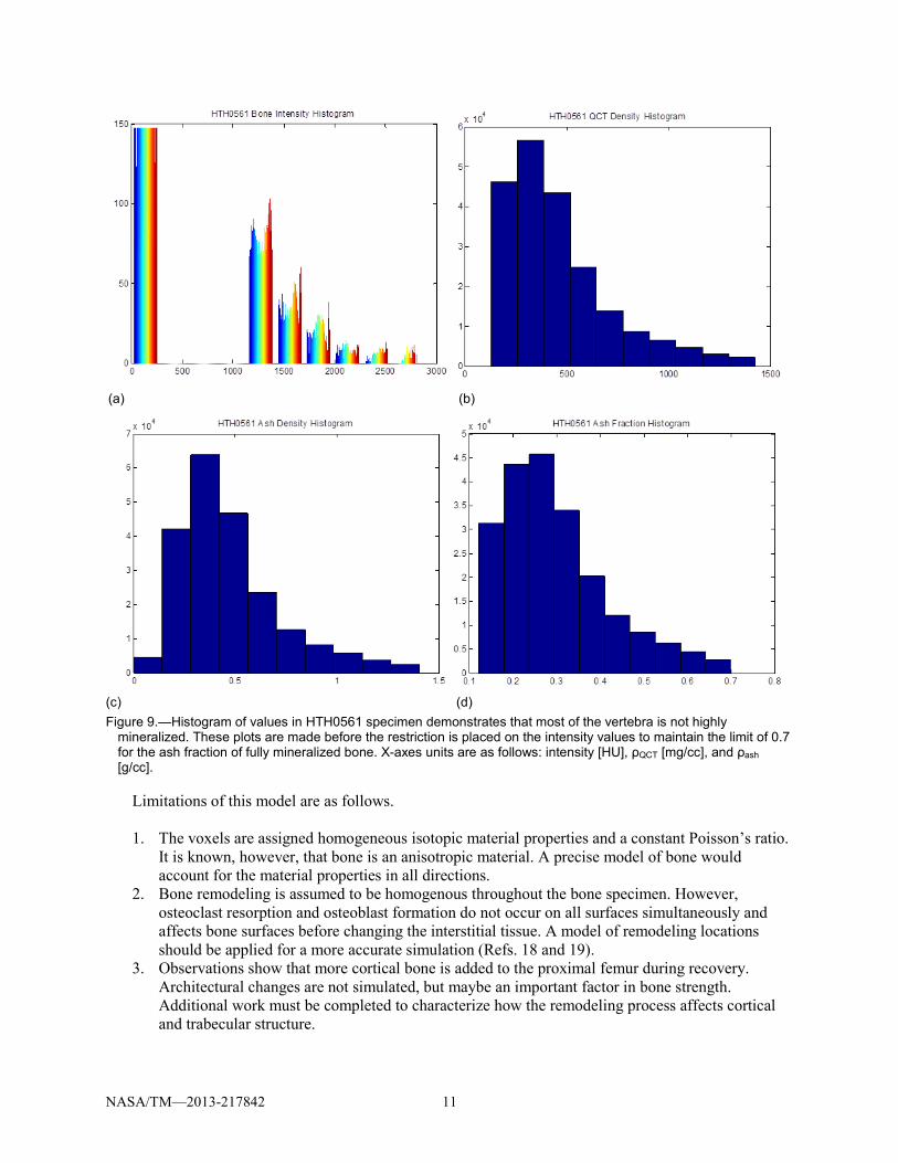
The T8 mean ash fractions indicate a higher osteoid volume fraction or a higher rate of bone remodeling at the time of scanning. The data were, therefore, re-analyzed to see if there was a problem in the image processing procedure. An intensity histogram shows one predominating region of intensity values around 1300 HU (Figure 9(a)). The first bar in the 0 to 200 HU is ignored because it is only counting the number of voxels in the background. The minimum intensity value of the entire bone specimen is found to be 1141.9 HU, which confirms the assumption of the first bar in bone intensity histogram.

An intensity histogram of a whole bone specimen should indicate two distinct parts—one for osteoid near the minimum intensity and one for fully mineralized bone near the maximum intensity. However, there is a single large grouping near the minimum intensity for all T8 specimens (Figure 9(a)). Hence, the ash fraction histogram only shows one distinct region with a low ash fraction corresponding to more osteoid (Figure 9(d)). Placing the intermediate calculations of QCT and ash density histograms shows that this is consistent throughout the calculation process from intensity values to ash fraction (Figure 9). There is no indication that there is a problem in the image processing functions.

The image processing procedure is further analyzed to see if the ROI size affects BVF and ash fraction. ROI size does affect the bone threshold value—the smaller the ROI, the smaller the threshold (Table 4). Higher threshold corresponds to higher ash fraction, but it removes more voxels from the images. It also has the potential to decrease the BVF significantly as seen in specimens HTH0243, HTH0339, and HTH0439 (Appendix D, Figure 12).

TABLE 4.—ASH FRACTION AND BVF ARE DEPENDENT ON THE IMAGE PROCESSING TYPE [Method A uses a fixed square ROI of 25 pixel length. Method B is a freehand ROI of the background.]

Specimen no. A: Threshold B: Threshold A: BVF0 B: BVF0 A: αmean0 B: αmean0 HTH0243 1127.9 1204.7 0.768 0.527 0.272 0.412 HTH0249 1114.6 1139.0 0.756 0.709 0.280 0.308 HTH0339 1099.1 1221.1 0.719 0.353 0.257 0.535 HTH0439 1092.7 1160.6 0.716 0.513 0.241 0.364 HTH0561 1140.9 1167.9 0.869 0.829 0.300 0.321

NASA/TM—2013-217842 11

(c) (d) Figure 9.—Histogram of values in HTH0561 specimen demonstrates that most of the vertebra is not highly

mineralized. These plots are made before the restriction is placed on the intensity values to maintain the limit of 0.7 for the ash fraction of fully mineralized bone. X-axes units are as follows: intensity [HU], ρQCT [mg/cc], and ρash [g/cc].

Limitations of this model are as follows. 1. The voxels are assigned homogeneous isotopic material properties and a constant Poisson’s ratio.

It is known, however, that bone is an anisotropic material. A precise model of bone would account for the material properties in all directions.

2. Bone remodeling is assumed to be homogenous throughout the bone specimen. However, osteoclast resorption and osteoblast formation do not occur on all surfaces simultaneously and affects bone surfaces before changing the interstitial tissue. A model of remodeling locations should be applied for a more accurate simulation (Refs. 18 and 19).

3. Observations show that more cortical bone is added to the proximal femur during recovery. Architectural changes are not simulated, but maybe an important factor in bone strength. Additional work must be completed to characterize how the remodeling process affects cortical and trabecular structure.

(a) (b)

NASA/TM—2013-217842 12

Axial rigidity provides a prediction of vertebral bone strength. This approach is limited because it assumes that minimum rigidity is an indicator of strength and does not consider deformations through the whole bone. Validation of the axial rigidity results cannot be made even though the T8 vertebrae are a subset of samples used in a previous study (Ref. 11). There is an error in the ash density and QCT density in the published paper. The coefficient of QCT density should be 0.95 not 9.5. It is unknown if this error persisted throughout the study. Hernandez et al. also did not use a two-parameter modulus equation to calculate the axial rigidity. Significant variations have been observed when using different equations to calculate elastic modulus (Appendix E, Figure 14).

The present work is successful in establishing a methodology to determine computational model input parameters from QCT images, to predict time-dependent changes to elastic modulus via the outputs of the cellular dynamics model, and to evaluate bone strength during bone loss and recovery using the initial bone strength as a baseline. An equation has been derived to obtain ash fraction values from QCT images, a good alternative for non-invasive studies and applications. This theoretical model combining the bone remodeling process with strength analysis may help provide guidance on normal 1 g activities to avoid during recovery and may help develop a bone loss prevention plan, particularly if used in conjunction with NASA’s probabilistic risk assessment of bone fracture risk (Ref. 20).

An extension of this study is to extend the simulation duration to include extreme long-duration space missions. NASA plans to send astronauts to Mars for a three year mission. However, American astronauts have spent at most 6 months in microgravity. The computational model would need to have built in ability to handle aging changes over longer time simulations and validated to be able to predict the amount of bone loss for 1000 days in a microgravity environment. An additional consideration for a Mars bone loss study is whether or not the 0.38 g environment will provide sufficient skeletal stimulation to help prevent bone resorption.

Prediction of bone recovery also contributes a better understanding of bone diseases here on Earth. Osteoporosis affects 10 million individuals in the United States alone, and 34 million more are estimated to have low bone density, placing them at an elevated risk for bone diseases and fractures (Ref. 21). An attribute of osteoporosis is marked reduction in bone mass due to an imbalance in the bone remodeling cycle. Modeling the physiological mechanics of bone may help to provide guidance for low bone density patients on what activities to avoid. Also, due to associated balance deficits, many elderly individuals tend to slip and fall on their hips, causing impact loading and fractures. That and the fact that astronauts lose bone mineral density in the proximal femur provide justification for extending this study to that anatomical location.

NASA/TM—2013-217842 13

.—Acronyms and Definitions Appendix A Acronyms A.1

BMC bone mineral content

BMU basic multicellular units

BVF bone volume fraction

DAP Digital Astronaut Project

DXA dual energy x-ray absorptiometry

FE finite element

FEM finite element models

HU Hounsfield units

QCT quantitative computed tomography

ROI region of interest

T8 eighth thoracic vertebra

A.2 Definitions

apparent ash density ρash inorganic mass / total volume

ash fraction α ash mass / dry bone mass

BMC mass of mineral measured from CT scans

BVF or BV/TV bone volume / total volume

dry apparent density ρapp (organic + inorganic mass) / total volume

Hounsfield units units of CT image numbers

mineralized bone organic + inorganic + water

QCT density ρQCT density determined from calibration phantom; only quantifies inorganic mineral component

NASA/TM—2013-217842 15

.—Remodeling QCT FEM Outline Appendix BNote: This process is automated in the remodelingMain.m. Refer to Appendix F for a README of the

MATLAB functions. 1. Determine mineral density calibration from calibration phantom image. 2. Process QCT image. Remove noise from liquid medium, and isolate bone from background. Obtain

3–D matrix mesh. 3. Calculate BVF either from 3–D matrix mesh for cubic volume sample or using Matlab Image

Processing Toolbox, specifically built-in functions ‘strel’ and ‘imclose’, for whole bone sample. 4. Calculate ash fraction (see derivation in Appendix C).

1.29α2 + 1.41α − ρash𝐵𝑉𝐹

= 0

(Note: ρash calculated from QCT density and ash density relation. BVF obtained from previous step.) 5. Run InitialValues.m to get rate of formation (rof), rate of resorption (ror), initial mature bone fraction

(Mo), initial osteoid fraction (Oo), and mineralization rate (Min_rate). 6. Set outputs of InitalValues.m in Set_InitalConditions.m. Run Set_InitalConditions.m. 7. Run BRequilibrium.m to get equilibrium conditions. 8. Create initial FEM from QCT. Voxel elastic modulus values determined from QCT density, ash

density, and modulus relations presented in Kaneko et al. and Keller papers. Run Abaqus Standard Analysis to obtain initial bone mechanics state.

9. Run BRmodeltrabecular.m to get time histories of relative mature bone fraction, osteoid fraction, and BVF saved in timeHistories.mat file.

10. Use Hernandez’s two-parameter power law to calculate modulus time history for each voxel at 10 day increments.

𝐸(𝑡) = 84.37 𝐵𝑉𝐹(𝑡)2.58 α(𝑡)2.74 [GPa]

11. Create FEM for x days using voxel modulus time history. Run Abaqus Standard Analysis and data processing to determine the biomechanical state at x days.

NASA/TM—2013-217842 17

.—Derivation of Equations Appendix CC.1 Ash Fraction

𝐵𝑉𝐹 ≈ρ𝑎𝑝𝑝�

gcc�

1.41+1.29α (Ref. 6)

ρapparent ash �gcc� = αρapparent � g

cc� (Ref. 7)

Combine above equations to get a function in terms of ash fraction only.

𝐵𝑉𝐹 =

ρash � gcc�

α1.41 + 1.29α

α(1.41 + 1.29α)𝐵𝑉𝐹 = ρash �gcc�

1.29α2 + 1.41α −ρash � g

cc�𝐵𝑉𝐹

= 0

Note: Ash fraction equation does not output imaginary ash fractions unless the ash density is negative, which is usually not the case since calibration phantom densities are 0 mg/cc or greater.

C.2 Maximum Intensity Value Corresponding to Ash Fraction of 0.7

1.29α2 + 1.41α −ρash � g

cc�𝐵𝑉𝐹

= 0

α(1.41 + 1.29α)𝐵𝑉𝐹 = ρash �gcc�

Equate with Ash Density and QCT Density Relation: Note: ρQCT has units of mg/cc.

K2HPO4 phantom CHA phantom

𝐵𝑉𝐹(1.29α2 + 1.41α) = 0.000953ρ𝑄𝐶𝑇 + 0.0457 𝐵𝑉𝐹(1.29α2 + 1.41α) = 0.000887ρ𝑄𝐶𝑇 + 0.0633

ρ𝑄𝐶𝑇 =𝐵𝑉𝐹(1.29α2 + 1.41α) − 0.0457

0.000953 ρ𝑄𝐶𝑇 =

𝐵𝑉𝐹(1.29α2 + 1.41α)− 0.06330.000887

Equate with Calibration Curve relating QCT density and Intensity Values: K2HPO4 phantom CHA phantom

𝑚𝑥 + 𝑏 = 𝐵𝑉𝐹(1.29α2 + 1.41α) − 0.0457

0.000953 𝑚𝑥 + 𝑏 =

𝐵𝑉𝐹(1.29α2 + 1.41α) − 0.06330.000887

𝑥 =1𝑚�

𝐵𝑉𝐹(1.29α2 + 1.41α) − 0.04570.000953 � − 𝑏 𝑥 =

1𝑚�

𝐵𝑉𝐹(1.29α2 + 1.41α) − 0.06330.000887 � − 𝑏

NASA/TM—2013-217842 18

Note: The above equations are only valid for linear correlation of QCT density with image intensity values. Keyak provided a L4 vertebra QCT image. A second order polynomial better describes the calibration plot for this particular specimen (Figure 10). However, the linear relation is not that far off. The maximum root of Equation (10) is taken to be the intensity value for an ash fraction of 0.7.

𝑎𝑥2 + 𝑏𝑥 + 𝑐 − 𝐵𝑉𝐹�1.29α2+1.41α�−0.06330.000887

= 0 (10)

Figure 10.—Calibration plot for CHA phantom for L4 vertebra from Keyak. A

second order plot better fits the plot of intensity values and known densities, but the linear relation is not that different.

1000 1050 1100 1150 1200 1250 1300 1350-20

0

20

40

60

80

100

120

140

160

Intensity

Den

sity

(mg/

cc)

Calibration Curve

Phantom CalibrationLinear Regression2nd Order Polynomial Regression

NASA/TM—2013-217842 19

.—Image Processing Method Appendix DNoise from the 20 percent ethanol bath and background is removed from the images to isolate the bone

specimen. Two sizes of ROIs are tested to assess the effect on ash fraction and BVF (Figure 11). Method A takes a fixed region of a 25 pixel length square. The user traces a region around the bone for Method B.

The bone threshold value is smaller using Method A rather than Method B. The processed images from Method A better retain the trabeculae in these T8 vertebrae (Figure 12). Method B’s threshold removes much of the trabeculae, decreasing the BVF significantly and increasing the ash fraction. HTH0339 midlayer slice best demonstrates the difference in image processing technique.

Figure 11.—Two sample sizes of the background are tested to see how it

affects the image: (a) uses a fixed square and (b) is done free-hand by the user.

Figure 12.—Collection of midlayer slices from all T8 vertebrae samples

demonstrates the effect of varying the background sample area during image processing.

NASA/TM—2013-217842 21

.—Justification of Voxel Material Property Equations Appendix ESeveral experimental studies characterize the QCT density from image technology with ash density

and elastic modulus. Appendix C summarizes these studies and validates the choice of relations used in this study.

A relation to convert QCT density to ash density is required to compute other parameters. Kaneko et al. studied the effect of metastases on the mechanical properties and densities of cortical and trabecular bone in the human femur (Refs. 12 and 13). The QCT density and ash density correlations were plotted for all four groups in the trabecular bone study: all data, no cancer, metastic lesions, and no lesions but died from cancer. The NC group equation does not diverge significantly from the All group equation until around 1400 mg/cc, which is a fairly high QCT density. It would also be acceptable to use the All group equation because the range of data from the NC group falls within the range of data from the All group. The cortical bone relations are also plotted, but do not yield similar trends in the All and no cancer groups. Since there is a significant disparity between the two equations, no cortical bone relation for QCT density to ash density is reported.

Keyak et al. combined the results from Kaneko et al.’s two studies and formulated a single ash density and QCT density relation (Ref. 14). This equation correlates well within the range of trabecular and cortical bone data (Figure 13). It must be noted that this equation does include data from bone samples with metastases. This equation would be beneficial to have a relation describing both types of bone.

Figure 13.—Cortical equations from Kaneko et al. 2003; trabecular equations from Kaneko et al. 2004

studying bone with and without metastases. N.S. indicates that the relation is not significant due to the small sample size. Solid lines are used to indicate the range of data; dashed lines indicate data extrapolation.

0 200 400 600 800 1000 1200 14000

200

400

600

800

1000

1200

1400

ρQCT [mg/cm3]

ρ ash

[mg/

cm3 ]

Ash density and QCT density relations for bone

Cortical AllCortical NC (N.S.)Cortical MLCortical NL (N.S.)Trabecular AllTrabecular NCTrabecular LTrabecular NLKeyak et al 2005

NASA/TM—2013-217842 22

A two-part ash density and QCT density relation can be used in later projects once more knowledge is known on how to identify cortical and trabecular bone from CT scans. A crude method to identify cortical from trabecular bone is to make mashed images of one of the other and then assign these voxels identifiers, so that the two types of bone can be assigned different material properties in the Abaqus input file. However, a main issue with this method is the fact that one cannot determine if a voxel is cortical or trabecular simply from looking at the QCT scan.

Analysis of the bone biomechanics is achieved using the elastic modulus, a parameter that measures a material’s ability to deform under particular loads. Several potential modulus equations have been considered (Figure 14). This study does not use modulus relations for only cortical or trabecular bone. The final verdict was to use the two-parameter modulus equation by Hernandez et al., which is not plotted in Figure 14 (Ref. 6). Keyak et al. equation would be ideal. However, if Keyak et al. relation is used to calculate the initial conditions, a discontinuity occurs within the first 10 days. No change in the BVF and ash fraction within the first 10 days implies that the modulus should also not change. Therefore, the two-parameter equation is used for consistency. Another reason for this decision is that the Keyak et al. modulus correlation was derived from data including bone metastasis samples. Since no correlation was shown between no cancer and metastasis groups in cortical bone, it would be better to use the two-parameter modulus equation (Ref. 12).

Figure 14.—Modulus and QCT density/Ash density relations show the diversity in equations. The two-parameter

Hernandez equation is not plotted here because QCT density is not its primary independent variable.

0 200 400 600 800 1000 1200 14000

5

10

15

20

25

30

ρQCT [mg/cm3]

Ela

stic

Mod

ulus

[GP

a]

Modulus correlations with ρQCT and ρash relation

Cortical N.S. (Kaneko et al. 2005)Mean for Trabecular (Kaneko et al. 2004)Trabecular (Keller 1994)All Bone (Keller 1994)All Bone (Keyak et al. 2005)

NASA/TM—2013-217842 23

.—Read Me for MATLAB Programs Appendix FRequired Software: • MATLAB (functions were written with version R2012.a) • MATLAB Image Processing Toolbox 8.0 • MATLAB Image Acquisition Toolbox 4.3

Optional Software: • ABAQUS—required for FEM (see Addition points section to comment MATLAB functions that

call ABAQUS)

The main function is remodelingMain.m. It is broken down into the following sections and automatically calls the relevant functions.

• Calibration Phantom Curve • uCT/QCT Processing and Initial Meshing • Initial FEM and Equilibrium State • Simulation of Bone Loss and Recovery • Results Processing

User inputs are required during this process in particular for image processing. They are indicated in

the command window with an arrow (Figure 15).

Figure 15.—Example of user inputs when running remodelingMain.m. This one requires the selection of fluid in

calibration phantom chamber.

NASA/TM—2013-217842 24

Some variables must be initialized before running remodelingMain.m.

• QCTtype—calibration phantom type: 1 for K2HPO4, 2 for CHA • boneType—simulation type: 1 for whole bone specimen, 2 for ROI • voxsize—voxel size [mm] • numcoarsen—number of voxels on an edge to combine (particularly useful for large FEMs to

reduce computational time) • sliceThickness—distance between layers of QCT [mm] • cubeLength—ROI vertical length [mm]; used for boneType option 2 • nu_bone—Poisson’s ratio of bone • bcType—type of fixed boundary condition on distal end of FEM: 1 for pin & roller, 2 for pin • Path locations

○ mechanotransductionModelFolder—location of mechanotransduction model MATLAB files

○ abaqusFolder—location to save INP, Abaqus analysis files, and MATLAB workspace ○ CTFolder—location of CT images

F.1 Calculating Voxel Size

If the voxel size is unknown, open a slice of the QCT in ImageJ. Under the filename in the upper left corner, there might be a line listing the image size and the number of voxels in the format 0.00- by 0.00-mm (000 by 000) (Figure 16). Use these values to calculate the voxel size.

F.1.1 Location of CT Images Upon running remodelingMain.m, the user will be prompted to choose a folder containing the CT

images. A single stack of QCT images should be placed in a folder with the specimen name. The program is automated to analyze multiple stacks of QCT images that use the same phantom. If the user would like to perform more than one specimen analysis, each specimen folder should be placed in a primary folder.

F.1.2 Modifications to Bone Remodeling Computation Model

If modifications are made to the mechanotransduction model, the user simply needs to make the changes in the respective functions. InitialValues.m and Set_InitialConditions.m from the original computation model have been incorporated into the remodelingMain.m function in “Initialize these Variables” and “Initial FEM and Equilibrium State” sections respectively.

Figure 16.—One slice of the QCT.

NASA/TM—2013-217842 25

F.1.3 Additional Points to be Aware of • The user must make sure that the calibration phantom curve is accurate for a particular set of

QCT images. It is advised to modify the calibrationphantom.m function after plotting different curves to the plot of mineral densities versus intensity values.

• If the user does not want to use Abaqus, comment the lines with the following functions in sections “Initial FEM and Equilibrium State” and “Simulation of Bone Loss and Recovery” of remodelingMain.m: ○ cd([abaqusFolder '\' nameFolders{#} '\' folder(#,:)]); ○ AbaINP(inpname(#,:),meshCT,thresh,voxsizeFE,sliceThickness,ini

tE,nu_ ○ bone,forceZ,sigmaZ,bctype); ○ pythonAbaqusScript(inpname(#,:),[abaqusFolder '\'

nameFolders{i} '\' ○ folder(#,:)]); ○ DATfile = [inpname(1,1:end-4) '.dat']; ○ effStrain(#,i) = DATProcessing(DATfile,[abaqusFolder '\' ○ folder(#,:)]);

F.2 List of MATLAB Functions Required for Remodeling Program remodelingMain.m

Image Processing:

• calibrationPhantom.m • coremeshQCT.m

FEMP:

• coarsen.m • AbaINP.m • im2h8.m • bc3.m • writeAbaH8.m • pythonAbaqusScript.m

Results Processing:

• compositeRigidity.m • DATProcessing.m

Mechanotransduction Model:

• BRequilibrium.m • BRequilibrium_rhs.m • BRmodeltrabecular.m • BRmodel_trabecular_rhs.m • depthF.m • depthR.m • dR.m • dA.m

NASA/TM—2013-217842 26

• g.m • Fa.m (updated in remodelingMain.m)

F.3 List of Current Results Outputted From remodelingMain.m

• Axial rigidity time history in kN • Relative Osteoid Volume Fraction • Relative Mineralized Volume Fraction • Relative Bone Volume Fraction • Ash Fraction

NASA/TM—2013-217842 27

.—Study of the Proximal Femur Appendix GMethodology to study the proximal femur during prolonged unloading and recovery is similar to the

one created using the thoracic vertebra. The primary difference is the physiological boundary conditions. Loading conditions for a normal 1 g single-stance loading condition is described here. Another important condition to consider is fall onto the greater trochanter.

Keyak et al. and Hazelwood et al. studied the proximal femur in response to long-term spaceflight and marathon training respectively (Ref. 22 and 15). Both FEM methods fully constrained the distal end of the femur. However, a pin and roller boundary condition is applied to the distal end of this study’s FEMs. The primary reason is that the femur rests on top of a cartilaginous tissue, which is a viscous material allowing movement in the lateral direction. Two nodes on the distal surface are also constrained in all coordinate directions to prevent the models from moving freely. The remaining nodes are only constrained in the z-direction to simulate rollers.

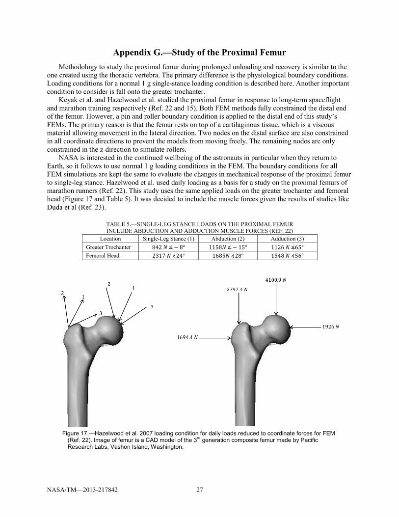
NASA is interested in the continued wellbeing of the astronauts in particular when they return to Earth, so it follows to use normal 1 g loading conditions in the FEM. The boundary conditions for all FEM simulations are kept the same to evaluate the changes in mechanical response of the proximal femur to single-leg stance. Hazelwood et al. used daily loading as a basis for a study on the proximal femurs of marathon runners (Ref. 22). This study uses the same applied loads on the greater trochanter and femoral head (Figure 17 and Table 5). It was decided to include the muscle forces given the results of studies like Duda et al (Ref. 23).

TABLE 5.—SINGLE-LEG STANCE LOADS ON THE PROXIMAL FEMUR INCLUDE ABDUCTION AND ADDUCTION MUSCLE FORCES (REF. 22)

Location Single-Leg Stance (1) Abduction (2) Adduction (3) Greater Trochanter 842 𝑁 ∡− 8° 1158𝑁 ∡− 15° 1126 𝑁 ∡65° Femoral Head 2317 𝑁 ∡24° 1685𝑁 ∡28° 1548 𝑁 ∡56°

Figure 17.—Hazelwood et al. 2007 loading condition for daily loads reduced to coordinate forces for FEM

(Ref. 22). Image of femur is a CAD model of the 3rd generation composite femur made by Pacific Research Labs, Vashon Island, Washington.

NASA/TM—2013-217842 28

MATLAB functions to apply the single-leg stance loading condition were not written because no QCT of the femur was obtained during the time of study. However, a theoretical approach was established. To determine the surface nodes, two transverse slices from the proximal end are taken at a time. Intersect of the two layers are declared as nodes of the surface of the femur (Figure 18). The process is repeated up to the diaphysis.

All the surface nodes have been identified. However, it is uncertain at this point which nodes are on the femoral head or the greater trochanter surfaces. Identification can be made by seeing which side of the centroid the nodes are located. If the nodes have a y-coordinate value greater than the centroid’s, then the nodes are placed in a node set for the femoral head. Again, QCT images of the proximal femur are integral to writing the MATLAB functions to apply boundary conditions to rounded surfaces.

Figure 18.—Illustration of how to determine which nodes are on surface of femoral head and greater trochanter. The

black region seen in the overlap of the two layers indicates the nodes that are on the surface where the single-stance loading condition will be applied.

NASA/TM—2013-217842 29

References 1. Sibonga, J.D., Evans, H.J., Sung, H.G., Spector, E.R., Lane, T.F., Ognaov, V.S., Bakulin A.V.,

Shackelford, L.C., LeBlanc, A.D. Recovery of spaceflight-induced bone loss: Bone mineral density after long-duration missions as fitted with an exponential function. Bone. 41 (2007): 973-978.

2. Lang, T.F., Leblanc, A.D., Evans, H.J., Lu, Y. Adaptation of the Proximal Femur to Skeletal Reloading After Long-Duration Spaceflight. Journal of Bone and Mineral Research. 21 (2006): 1224-1230.

3. Pennline, J.A. Simulating Bone Loss in Microgravity Using Mathematical Formulations of Bone Remodeling. Washington, D.C.: National Aeronautics and Space Administrations. NASA TM—2009-215824. November 2009.

4. Frost, H.M. Bone “mass” and the “mechanostat”: a proposal. The Anatomical Record. 219 (1987): 1-9. 5. Frost, H.M. Bone’s mechanostat: A 2003 update. The Anatomical Record. 275A (2003): 1081-1101. 6. Hernandez, C.J., Beaupré, G.S., Keller, T.S., Carter D.R. The Influence of Bone Volume Fraction and

Ash Fraction on Bone Strength and Modulus. Bone. 29 (2001): 74-78. 7. Keller, T.S. Predicting the compressive mechanical behavior of bone. Journal of Biomechanics. 27

(1994): 1159-1168. 8. Pennline, J.A. Personal Communication. June - August 2012. In publication phase. 9. Cody, D.D., Gross, G.J., Hou, F.J., Spencer, H.J., Goldstein, S.A., Fyhrie, D.P. Femoral strength is

better predicted by finite element models than QCT and DXA. Journal of Biomechanics. 32 (1999): 1013-1020.

10. Keyak, J.H., Koyama, A.K., LeBlanc, A., Lu, Y., Lang, T.F. Reduction in proximal femoral strength due to long-duration spaceflight. Bone. 44 (2009): 449-453.

11. Hernandez, C.J., Loomis, D.A., Cotter, M.M., Schifle, A.L., Anderson, L.C., Elsmore, L., Kunos, C., Latimer, B. Biomechanical allometry in hominoid thoracic vertebrae. Journal of Human Evolution. 56 (2009): 462-470.

12. Kaneko, T.S., Pejcic, M.R., Tehranzadeh, J., Keyak, J.H. Relationships between material properties and CT scan data of cortical bone with and without metastatic lesions. Medical Engineering & Physics. 25 (2003): 445-454.

13. Kaneko, T.S., Bell J.S., Pejcic, M.R., Tehranzadeh, J., Keyak, J.H. Mechanical properties, density and quantitative CT scan data of trabecular bone with and without metastases. Journal of Biomechanics. 37 (2004): 532-530.

14. Keyak, J.H., Kaneko, T.S., Tehranzadeh, J., Skinner, H.B. Predicting Proximal Femoral Strength Using Structural Engineering Models. Clinical Orthopaedics and Related Research. 437 (2005): 219-228.

15. Keyak, J.H., Lee, I.Y., Skinner, H.B. Correlations between orthogonal mechanical properties and density of trabecular bone: Use of different densitometric measures. Journal of Biomedical Materials Research. 28 (1994): 1329-1336.

16. Whealan, K.M., Kwak, S.D., Tedrow, J.R., Inoue, K., Snyder, B.D. Noninvasive Imaging Predicts Failure Load of the Spine with Simulated Osteolytic Defects. The Journal of Bone & Joint Surgery. 82 (2000): 1240-1251.

17. Iyer, S., Christiansen, B.A., Roberts, B.J., Valentine, M.J., Manoharan, R.K., Bouxsein, M.K. A Biomechanical Model for Estimating Loads on Thoracic and Lumbar Vertebrae. Clinical Biomechanics. 25 (2010): 853-858.

18. Jaasma, M.J., Bayraktar, H.H., Niebur, G.L., Keaveny, T.M. Biomechanical effects of intraspecimen variations in tissue modulus for trabecular bone. Journal of Biomechanics. 35 (2002): 237-246.

19. van der Linden, J.C., Birkenhager-Frenkel, D.H., Verhaar, J.A.N., Weinans, H. Trabecular bone’s mechanical properties are affected by its non-uniform mineral distribution. Journal of Biomechanics. 34 (2001): 1573-1580.

20. Nelson, E.S., Lewandowski, B., Licata, A., Myers, J.G. Development and Validation of a predictive bone fracture risk model for astronauts. Annals of Biomedical Engineering. 37 (2009): 2337-2359.

NASA/TM—2013-217842 30

21. National Osteoporosis Foundation. “About Osteoporosis: Bone Basics—Fast Facts.” National Osteoporosis Foundation. n.d. Web. 5 Jul. 2012.

22. Hazelwood, S.J., Castillo A.B. Simulated effects of marathon training on bone density, remodeling, and microdamage accumulation of the femur. International Journal of Fatigue. 29 (2007): 1057-1064.

23. Duda, G.N., Schneider, E., Chao, E.Y.S. Internal forces and moments in the femur during walking. Journal of Biomechanics. 30 (1997): 933-941.

REPORT DOCUMENTATION PAGE Form Approved OMB No. 0704-0188

The public reporting burden for this collection of information is estimated to average 1 hour per response, including the time for reviewing instructions, searching existing data sources, gathering and maintaining the data needed, and completing and reviewing the collection of information. Send comments regarding this burden estimate or any other aspect of this collection of information, including suggestions for reducing this burden, to Department of Defense, Washington Headquarters Services, Directorate for Information Operations and Reports (0704-0188), 1215 Jefferson Davis Highway, Suite 1204, Arlington, VA 22202-4302. Respondents should be aware that notwithstanding any other provision of law, no person shall be subject to any penalty for failing to comply with a collection of information if it does not display a currently valid OMB control number. PLEASE DO NOT RETURN YOUR FORM TO THE ABOVE ADDRESS.

1. REPORT DATE (DD-MM-YYYY) 01-02-2013

2. REPORT TYPE Technical Memorandum

3. DATES COVERED (From - To)

4. TITLE AND SUBTITLE Predicting Bone Mechanical State During Recovery After Long-Duration Skeletal Unloading Using QCT and Finite Element Modeling

5a. CONTRACT NUMBER

5b. GRANT NUMBER

5c. PROGRAM ELEMENT NUMBER

6. AUTHOR(S) Chang, Katarina, L.; Pennline, James, A.

5d. PROJECT NUMBER

5e. TASK NUMBER

5f. WORK UNIT NUMBER WBS 516724.02.02.10

7. PERFORMING ORGANIZATION NAME(S) AND ADDRESS(ES) National Aeronautics and Space Administration John H. Glenn Research Center at Lewis Field Cleveland, Ohio 44135-3191

8. PERFORMING ORGANIZATION REPORT NUMBER E-18616

9. SPONSORING/MONITORING AGENCY NAME(S) AND ADDRESS(ES) National Aeronautics and Space Administration Washington, DC 20546-0001

10. SPONSORING/MONITOR'S ACRONYM(S) NASA

11. SPONSORING/MONITORING REPORT NUMBER NASA/TM-2013-217842

12. DISTRIBUTION/AVAILABILITY STATEMENT Unclassified-Unlimited Subject Categories: 39, 51, and 52 Available electronically at http://www.sti.nasa.gov This publication is available from the NASA Center for AeroSpace Information, 443-757-5802

13. SUPPLEMENTARY NOTES

14. ABSTRACT During long-duration missions at the International Space Station, astronauts experience weightlessness leading to skeletal unloading. Unloading causes a lack of a mechanical stimulus that triggers bone cellular units to remove mass from the skeleton. A mathematical system of the cellular dynamics predicts theoretical changes to volume fractions and ash fraction in response to temporal variations in skeletal loading. No current model uses image technology to gather information about a skeletal site’s initial properties to calculate bone remodeling changes and then to compare predicted bone strengths with the initial strength. The goal of this study is to use quantitative computed tomography (QCT) in conjunction with a computational model of the bone remodeling process to establish initial bone properties to predict changes in bone mechanics during bone loss and recovery with finite element (FE) modeling. Input parameters for the remodeling model include bone volume fraction and ash fraction, which are both computed from the QCT images. A non-destructive approach to measure ash fraction is also derived. Voxel-based finite element models (FEM) created from QCTs provide initial evaluation of bone strength. Bone volume fraction and ash fraction outputs from the computational model predict changes to the elastic modulus of bone via a two-parameter equation. The modulus captures the effect of bone remodeling and functions as the key to evaluate of changes in strength. Application of this time-dependent modulus to FEMs and composite beam theory enables an assessment of bone mechanics during recovery. Prediction of bone strength is not only important for astronauts, but is also pertinent to millions of patients with osteoporosis and low bone density.15. SUBJECT TERMS Bone mineral content; Microgravity; Mathematical model; Finite element method; Quantitative computer tomography; Simulation; Spine

16. SECURITY CLASSIFICATION OF: 17. LIMITATION OF ABSTRACT UU

18. NUMBER OF PAGES

38

19a. NAME OF RESPONSIBLE PERSON STI Help Desk (email:help@sti.nasa.gov)

a. REPORT U

b. ABSTRACT U

c. THIS PAGE U

19b. TELEPHONE NUMBER (include area code) 443-757-5802

Standard Form 298 (Rev. 8-98)Prescribed by ANSI Std. Z39-18