Predicting and Interpreting

Electron Paramagnetic Resonance Spectra.

Graeme R. Hanson

Centre for Magnetic Resonance,The University of Queensland, St. Lucia, Queensland, Australia, 4072.

Email: Graeme.Hanson@CMR.uq.edu.au Ph: +61-7-3365-3242, Fax: +61-7-3365-3833

Summary

1. Introduction into Computer Simulation of Continuous Wave (CW) EPR Spectra

2. Theory and Brief overview of Xsophe2.1 Theory used in Calculating a Simulated EPR Spectrum2.2 Field versus Frequency Swept EPR2.3 Numerical Integration - Choice of Angular Grid2.4 Transition Searching - Field Segmentation2.5 Linewidth Models2.6 Parallelisation2.7 Optimisation Methods2.8 Brief Product Overview of Xsophe

3. Role of frequency (and temperature) in extracting spin Hamiltonian parameters 3.1 Fine structure interaction 3.2 Isotropic and Anisotropic Exchange interactions 3.3 distributions of parameters

3.3.1 Distributions of g and A values - Examples - Low Spin Fe(III) and Co(II)Centres

3.3.2 Distributions of D and E values3.3.3 Energy level crossings and anticrossings and looping transitions

4. Role of frequency in spectral resolution

5. Summary

6. Acknowledgements

7. Bibliography

2

(1)

(2)

(3)

1. Introduction into Computer Simulation of Continuous Wave (CW) EPR Spectra

Multifrequency electron paramagnetic resonance (EPR) spectroscopy [1-7] is a powerful toolfor characterising paramagnetic molecules or centres within molecules that contain one or moreunpaired electrons. Computer simulation of the experimental randomly orientated or single crystalEPR spectra from isolated or coupled paramagnetic centres is often the only means available foraccurately extracting the spin Hamiltonian parameters required for the determination of structuralinformation [1,2,9-21].

2. Theory and Brief overview of XSophe

2.1 Theory used in Calculating a Simulated EPR SpectrumEPR spectra are often complex and are interpreted with the aid of a spin Hamiltonian. For anisolated paramagnetic centre (A) a general spin Hamiltonian is [1,2,8]:

where S and I are the electron and nuclear spin operators respectively, D the zero field splittingtensor, g and A are the electron Zeeman and hyperfine coupling matrices respectively, Q thequadrupole tensor, � the nuclear gyromagnetic ratio, � the chemical shift tensor, � the Bohrmagneton and B the applied magnetic field. Additional hyperfine, quadrupole and nuclear Zeemaninteractions will be required when superhyperfine splitting is resolved in the experimental EPRspectrum. When two or more paramagnetic centres (Ai, i = 1, ..., N) interact, the EPR spectrum isdescribed by a total spin Hamiltonian (�Total) which is the sum of the individual spin Hamiltonians(�Ai

, Eq. [1]) for the isolated centres (Ai) and the interaction Hamiltonian (�Aij ) which accounts

for the isotropic exchange, antisymmetric exchange and the anisotropic spin-spin (dipole-dipolecoupling) interactions between a pair of paramagnetic centres [1,9,10].

Computer simulation of randomly orientated EPR spectra is performed in frequency spacethrough the following integration [1,22]

where S(B,�c) denotes the spectral intensity, �µ ij�² is the transition probability, �c the microwavefrequency, �o(B) the resonant frequency, �v the spectral line width, ƒ[�c - �o(B), �

�] a spectral

lineshape function which normally takes the form of either Gaussian or Lorentzian, and C a constantwhich incorporates various experimental parameters. The summation is performed over all thetransitions (i, j) contributing to the spectrum and the integrations, approximated by summations, areperformed over half of the unit sphere (for ions possessing triclinic symmetry), a consequence oftime reversal symmetry [1,8]. For paramagnetic centres exhibiting orthorhombic or monoclinicsymmetry, the integrations in Eq. [3] need only be performed over one or two octants respectively.Whilst centres exhibiting axial symmetry require integration only over �, those possessing cubicsymmetry require only a single orientation.

3

(4a)

(4c)

(4b)

2.2 Field versus Frequency Swept EPRIn practice the EPR experiment is a field swept experiment in which the microwave frequency

(�c) is kept constant and the magnetic field varied. Computer simulations performed in field spaceassume a symmetric lineshape function f in Eq. [1] (f(B-Bres), �B) which must be multiplied byd�/dB and a constant transition probability across a given resonance.[1,22] In fact Pilbrow hasdescribed the limitations of this approach in relation to asymmetric lineshapes observed in high spinCr(III) spectra and the presence of a distribution of g-values (or g-strain broadening). The followingapproach has been employed by Pilbrow et al. in implementing Eq. [1] (frequency swept) intocomputer simulation programmes based perturbation theory [1,9]. Firstly, at a given orientation of(�, �), the resonant field positions (Bres) are calculated with perturbation theory and thentransformed into frequency space (�0(B)). Secondly, the lineshape (f(�c-�0 (B), �

�) and transition

probability are calculated in frequency space across a give resonance and the intensity at eachfrequency stored. Finally, the frequency swept spectrum is transformed back into field space.Performing computer simulations in frequency space produces assymmetric lineshapes (withouthaving to artificially use an asymmetric lineshape function) and secondly, in the presence of largedistribution of g-values will correctly reproduce the downfield shifts of resonant field positions.[9]

Unfortunately, the above approach cannot be used in conjunction with matrix diagonalizationas an increased number of matrix diagonalizations would be required to calculate f and thetransition probability across a particular resonance. However, Homotopy [46] which is in generalthree to five times faster than matrix diagonalization allows the simulations to be performed infrequency space.

2.3 Numerical Integration - Choice of Angular GridIn numerical terms, computer simulation of randomly oriented EPR spectra involves the

calculation of the resonant field positions and transition probabilities at all vertex points of a givenpartition for all contributing transitions. The simplest and most popular partition scheme is that ofusing the geophysical locations on the surface of the Earth for the presentation of world maps.However, the solid angle subtended by the grid points is uneven and alternative schemes have beeninvented and used in the simulation of magnetic resonance spectra. For example, in order to reducecomputational times involved in numerical integration over the surface of the unit sphere, the igloo[19], triangular [24] and spiral [25] methods have been invented for numerical investigations ofspatial anisotropy. In 1995, we described a new partition scheme, the SOPHE partition scheme [16]in which any portion of the unit sphere (� � [0, �/2], � � [�1, �2 ] or � � [�/2, �], � � [�1, �2])can be partitioned into triangular convexes. For a single octant (� � [0, �/2], � � [0, �/2]) thetriangular convexes can be defined by three sets of curves

where N is defined as the partition number and gives rise to N+1 values of �. Similar expressionscan be easily obtained for � � [�/2, �], � � [�1, �2]. A three dimensional visualisation of theSOPHE partition scheme is given in Figure 1b.

4

Figure 1. A schematic representation of the SOPHE partition scheme. (a) Vertex points with aSOPHE partition number N = 10; (b) the SOPHE partition grid in which the three sets of curves aredescribed by Eq. [4]. (c) Subpartitioning into smaller triangles can be performed by using either Eq.[4] or alternatively the points along the edge of the triangle are interpolated by the cubic splineinterpolation method [24] and each point inside the triangle is linearly interpolated three times andan average is taken.

As can be seen this method partitions the surface of the unit sphere into triangular convexes whichresemble the roof of the famous Sydney Opera House. In SOPHE there are N curves in each setwith the number of grid points varying from 2 to N+1 in steps of 1. In order to produce simulatedspectra of high quality, the unit sphere is often required to be finely partitioned, in other words, alarge number of vertex points are required. Each triangle in Figure 1b can be easily subpartitionedinto smaller triangles, referred to as tiny triangles. In Figure 1c, a selected triangle is furtherpartitioned into 81 tiny triangles with a subpartion number M=10. The grid formed in such asubpartition can still be described by Eq. [4]. In this particular case, � is stepped in a smaller step of�/(2(N-1)*(M-1)) from �= 45o to �= 54o, the two corresponding curves which bound the triangle(Figure 1c). A similar process is applied to curves in sets 2 and 3. Solid angles for these tinytriangles can be calculated from Eq. [5]. Alternatively, various interpolation schemes may be usedfor simulating randomly oriented EPR spectra [20,24-26]. Recently, we developed a highly efficientinterpolation scheme, the SOPHE interpolation scheme [16].

The SOPHE interpolation scheme is divided into two levels of interpolation, a globalinterpolation using cubic spline [27] and a local interpolation using simple linear interpolation.Given the function values which may represent the resonant field position or the transitionprobability at the vertex points (Figure 1a), we use the cubic spline interpolation method tointerpolate the function values at all other points on the curves described by Eq. [4] (Figure 1b).This is actually carried out in three different sets. In each set, there are N interpolations with thenumber of knots (vertex points) varying from 2 to N+1. Although in two of the three sets (Eqs. 4band 4c) both variables � and � are involved, variable � can be treated as a parameter [16]. Firstderivative boundary conditions [27] have been employed in our program which has been proved toproduce high-quality interpolated data [16].

5

(5)

After the global interpolation, the integration over the unit sphere can be viewed as integratingthrough individual triangularly shaped convexes. A second level of interpolation is carried out basedon the values globally interpolated and this is schematically shown in Figure 1c. The resonant fieldposition and transition probability are calculated at the vertices (tiny triangles) formed by linearinterpolation (up to version 1.0.2) of the points on adjacent sides of the triangular convex. This isrepeated for the other two pairs of sides of the triangular convex and the results averaged. Linearinterpolation is based on a subpartition scheme and each triangular convex can be subpartitioneddifferently[16]. Intuitively speaking, the global cubic spline interpolation can be viewed as buildingup a “skeleton” based on the SOPHE grid and the local linear interpolation can be viewed as a “tilefilling process”. In the early versions of XSophe we assume all the tiny triangles in a given trianglesubtend the same solid angle. In version 1.0.4 of XSophe we calculate the exact areas and use cubicspline interpolation for the tile filling process.

An example demonstrating the efficiency of the SOPHE partition and interpolation schemes isshown in Figure 2 where we have calculated a randomly orientated spectrum for a high spinrhombically distorted Cr(III) ion for which an appropriate spin Hamiltonian is

The spin Hamiltonian parameters employed were ge = 1.990, D = 0.10 (cm-1), E/D = 0.25, gn = 1.50,Ax = 120, Ay = 120, Az = 240 (10-4 cm-1). A narrow line width was chosen (30 MHz) in order todemonstrate the high efficiency of these schemes. The unit sphere has to be partitioned very finelyin order to produce simulated spectra with high signal to noise ratios when there is large anisotropyand the spectral linewidths are narrow. The simulated spectra without and with the SOPHEinterpolation scheme with a partition number N=18 are shown in Figures 2a and 2b respectively.

Figure 2. Computer simulations of the powder EPRspectrum from a fictitious spin system (S=3/2; I=3/2) whichdemonstrates the efficiency of the SOPHE interpolationscheme. (a) Without the SOPHE interpolation scheme,N=18, (b) With the SOPHE interpolation scheme, N=18 and(c) Without the SOPHE interpolation scheme, N=400. Thecomputational times were obtained on a SGI O2 R5K (180MHz). �=34 GHz; field axis resolution: 4096 points; anisotropic Gaussian lineshape with a half width at halfmaximum of 30 MHz was used in the simulation.

6

Without the SOPHE interpolation scheme, the spectral information is completely lost in the sea ofcomputing noise (computational time was 29.36 sec.) whereas with the SOPHE interpolationscheme, a virtually noise-free spectrum was produced in 63.11 sec. In order to appreciate this better,a simulation without interpolation with a much larger partition number (N=400) produced aspectrum of lower quality (Figure 2c) and consumed 3 hrs. 47.94 min. of CPU time. To make thecomparison in more detail, for Figure 2b an average of 5.6 million data points were generatedthrough the SOPHE interpolation scheme for each of the 12 allowed transitions whereas for Figure2c there were only 80,200 data points, a mere portion of the interpolated points. Clearly, spectra ofcomparable quality can be simulated with the SOPHE interpolation scheme at a significantlyreduced computational time by approximately two orders of magnitude.

The use of the SOPHE interpolation scheme significantly reduces the time-consumingprocess of locating the resonance field positions and evaluation of the transition probabilities in thefull matrix diagonalization. Having demonstrated the advantages of the SOPHE interpolationscheme, we should also point out its limitations. Firstly, the interpolation scheme will fail whenthere are multiple resonant field positions present at a given orientation (�, �) and when loopingtransitions are present. We have implemented two solutions to solve these problems. The user canuse the brute force matrix diagonalization or alternatively homotopy.[46]

2.4 Transition Searching - Field SegmentationThe very nature of EPR spectroscopy as a field-swept technique imposes a computational

challenge to computer simulation of randomly oriented spectra. In essence, during an EPRexperiment, the spin system under investigation is constantly modified through the Zeemaninteractions as the magnetic field is swept. In a general situation where two or more interactionshave comparable energies, search for resonance field positions is not a trivial task as the dependenceof the energies of the spin states on field strength ( B0 ) can be very complex. The complicationinvolved is best manifested by the presence of multiple transitions between a given pair of energylevels.

A number of search schemes have been used in the full matrix diagonalization approach forlocating resonance field positions [14,20,28-30]. Generally, they can be grouped into twocategories. In category I, the resonance field position is searched independently for every transition.Among the schemes belonging to this category, the so-called iterative bisection method is the safestbut probably the most inefficient method [14]. Other more efficient methods such as the Newton-Raphson method have also been used [14]. In general, these search schemes are time-consumingas a large number of diagonalizations are normally required. The search schemes belonging tocategory II may be called segmentation methods. In these schemes, the field sweep range is dividedequally into K segments and for each segment, the whole energy matrix is diagonalised once for thecentre field value of that segment. Thus only K diagonalizations are performed for each orientation.A perturbation theory is then employed for determining the presence of a transition in each segment.This search scheme is still limited to situations where in each segment there is no more than onepossible transition. However, if K is not too small, the chance of having two resonances in a singlesegment is rare. Reijerse et al. [20] use a first-order perturbation approach for exploring transitionsin each segment. However, from our experience, first-order perturbation theory cannot beguaranteed to produce resonance field positions with satisfactory precision. In Sophe we haveadopted the second-order eigenfield perturbation theory originally developed by Belford et al [31] inour program which has also been used by other groups[29]. The segment number, K, is a user-inputparameter. We have found that second-order eigenfield perturbation theory used in conjunction withour segmentation scheme cannot only deal with complicated situations such as multiple transitionsbut also proved to be efficient and reliable for locating the resonance field positions in field-sweptEPR spectra.

7

(6)

(7)

(8)

A saving factor in the segmentation method lies in the fact that full matrix diagonalization isonly performed K times irrespective of the number of transitions involved. By contrast, in the otherschemes, a few diagonalizations are required for each transition and for large spin systems thisnumber can become very large. The precision of the resonance field positions normally depends onthe segment number K as well as on the spin system. How large the segment number should bedepends on the nature of the system under study. However, simulations can be performed withdifferent segmentation numbers providing an easy test of precision.

2.5 Linewidth ModelsA number of linewidth models originally developed for magnetically isolated paramagnetic

species have been incorporated into the XSophe computer simulation software suite. For all thelinewidth models discussed below the linewidth parameter, �

� , is given in energy units. In Sophe

(field space version), �� is converted to a field-domain linewidth parameter �B through �B = |dB/dEij

|�� (where B is the magnetic field and Eij = Ei - Ej ) [1, 22]. |dB/dEij | is calculated for each transition

by using eigenfield perturbation theory [31]. The linewidth models incorporated into Sopheinclude:

� Kivelson's linewidth model [36] for isotropic spectra

The coefficients a, b, c, and d can be related to the solvent viscosity, correlation time,molecular hydrodynamics radius and the anisotropy of the spin system under study [36].

� Angular variation of the g-values [1].

where g2 = gx2 lx

2 + gy2 ly

2 + gz2 lz

2 , �i's (i=x,y,z) are the input linewidth parameters and li's(i=x,y,z) are the direction cosines of the magnetic field with respect to the principal axes ofthe g matrix.

� A correlated g-A strain model which was originally developed by Froncisz and Hyde [37] andhas been used successfully to account for the linewidth variations encountered in spin S=1/2systems particularly in copper and low spin cobalt ( S=1/2 ) complexes [1,3,37]. Whenexpressed in the frequency-domain [1,22], the linewidth in this model is based on theformulae

where the �Ri (i =x, y, z) are the residual linewidths due to unresolved metal and/or ligandhyperfine splitting, homogeneous linewidth broadening, and other sources, �gi's and �Ai'sare the widths of the Gaussian distributions of the g and A values. The g-A strain modelinvolves nine parameters for a rhombically distorted metal ion site.

� Wenzel and Kim [38] have described a statistical D-E strain model. In their model, thedistributions of D and E are assumed to be Gaussian and independent of each other with theresulting full width at maximum slope due to strain alone given by

8

(9)

(10)

(11)

where �D and �E are the half-widths at maximum slope of the distributions of D and E inenergy units, respectively, and �i and �j are the wavefunctions associated with transition i�j. A residual linewidth, �R, is convoluted with the D-E strain effects

2.6 ParallelisationWith the advent of multiprocessor computers and the new algorithms described above the

simulation of EPR spectra from complex spin systems consisting of multiple electron and or nuclearspins becomes feasible with Sophe. Optimisation of the spin Hamiltonian parameters by thecomputer will also be possible for these spin systems. Parallelisation of the matrix diagonalizationmethod has been performed at the level of the vertices in the Sophe grid. For example, if acomputer has 5 processors then the number of Sophe grid points is divided into groups of five andeach group is then processed by a one of the processors with the resultant spectra being added to anarray shared by the five processors. For the hypothetical Cr(III) spin system shown in Figure 2 athree-fold reduction in computational time is observed. Greater reductions are observed for morecomplex spin systems.

2.7 Optimisation MethodsA unique set of spin Hamiltonian parameters for an experimental EPR spectrum is obtained

through minimising the goodness of fit parameter (GF)

where the experimental spectrum (Yexp) has been baseline corrected assuming a linear baseline andthe simulated spectrum has been scaled () to Yexp. N is the number of points in common betweenthe experimental and simulated spectra and � is the magnitude of noise in the spectrum. In the pastminimising GF has been performed through a process of trial-and-error by visually comparing thesimulated and experimental spectra until a close match was found. Recent progress in reducingcomputational times for computer simulations (Sections 3-7) and the improved speed ofworkstations allows the use of computer-based optimisation procedures to find the correct set ofspin Hamiltonian parameters from a given EPR spectrum.

The most appropriate technique for optimising a set of spin Hamiltonian parameters isnonlinear least squares [40]. This method has the advantage that the differences (Yexp - S(B, �c), Eq.11) associated with the more extreme positive or negative values are exaggerated, which emphasisesgenuine peak mis-matching whilst tending to reduce the impact of noise. Unfortunately, evaluationof S(B, �c) can take a long time and as there is no analytic derivative information available, thismethod is not really an option for general spin systems. Consequently, we have considered threedirect methods, the Hooke and Jeeve's [42], Simplex [43] and a Quadratic method based on theHooke and Jeeves method and two simulated annealing approaches [46]. In addition there areseveral problems which need to be addressed, including (i) the sensitivity of scaling the various spinHamiltonian parameters and the method chosen for comparing the experimental simulated spectra[46]. In XSophe we allow the user to control the sensitivity of parameter adjustment throughout theoptimisation procedure and secondly the user can compare the spectra directly or the Fouriertransformed spectra. The latter method provides increased resolution through separating the high

9

and low frequency components [45]. As an aid to optimising the computer simulationXSophe/Xepr has the capability of displaying intermediate spectra (Magnetic Field vs. Intensity vs.Iteration Number) and the corresponding spin Hamiltonian parameters. Ideally, you would like tooptimise a set of multifrequency EPR spectra with a single set of spin Hamiltonian parameters.Although this can be achieved in the current version of Xsophe, the methodology is not straightforward. Version 2.0 of XSophe currently under development will allow this and the optimisationof multi-component spectra.

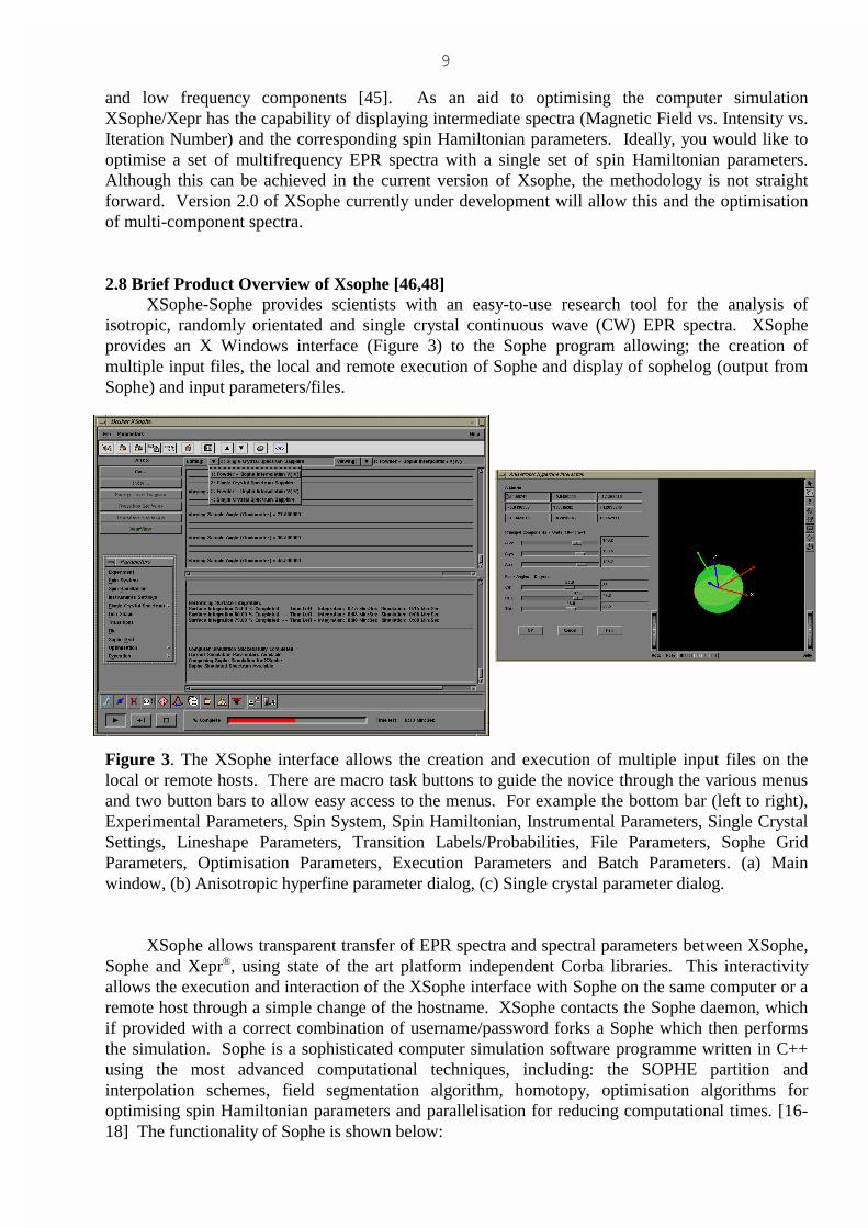
2.8 Brief Product Overview of Xsophe [46,48]XSophe-Sophe provides scientists with an easy-to-use research tool for the analysis of

isotropic, randomly orientated and single crystal continuous wave (CW) EPR spectra. XSopheprovides an X Windows interface (Figure 3) to the Sophe program allowing; the creation ofmultiple input files, the local and remote execution of Sophe and display of sophelog (output fromSophe) and input parameters/files.

Figure 3. The XSophe interface allows the creation and execution of multiple input files on thelocal or remote hosts. There are macro task buttons to guide the novice through the various menusand two button bars to allow easy access to the menus. For example the bottom bar (left to right),Experimental Parameters, Spin System, Spin Hamiltonian, Instrumental Parameters, Single CrystalSettings, Lineshape Parameters, Transition Labels/Probabilities, File Parameters, Sophe GridParameters, Optimisation Parameters, Execution Parameters and Batch Parameters. (a) Mainwindow, (b) Anisotropic hyperfine parameter dialog, (c) Single crystal parameter dialog.

XSophe allows transparent transfer of EPR spectra and spectral parameters between XSophe,Sophe and Xepr®, using state of the art platform independent Corba libraries. This interactivityallows the execution and interaction of the XSophe interface with Sophe on the same computer or aremote host through a simple change of the hostname. XSophe contacts the Sophe daemon, whichif provided with a correct combination of username/password forks a Sophe which then performsthe simulation. Sophe is a sophisticated computer simulation software programme written in C++using the most advanced computational techniques, including: the SOPHE partition andinterpolation schemes, field segmentation algorithm, homotopy, optimisation algorithms foroptimising spin Hamiltonian parameters and parallelisation for reducing computational times. [16-18] The functionality of Sophe is shown below:

10

Experiments� Energy level diagrams, transition surfaces, continuous wave EPR spectra, pulsed EPR

spectra under development.Spin Systems

� Isolated and magnetically coupled spin systems. An unlimited number of electron andnuclear spins is supported with nuclei having multiple isotopes.

� Interactions as listed in the following Table.

Table 1. Spin Hamiltonian Interactions included in Sophe.

Operator Form Description

S.B ( �e S.g.B) Electron Zeeman

I.B ( �n gn I.B) Nuclear Zeeman

S.D.S Fine structure

S4, S6 High-order fine structure*

I.P.I Quadrupole

S.A.I Hyperfine

Si . Jij . Sj Dipole Dipole

Jij Si . Sj Exchange

*All high-order fine-structure terms taken from Table 1 in reference [8] have beenincorporated into Sophe.

Continuous Wave EPR Spectra� Spectra types: Solution, randomly orientated and single crystal� Symmetries: Isotropic, axial, orthorhombic, monoclinic and triclinic� Multidimensional spectra: Variable temperature, multifrequency and the simulation of

single crystal spectra in a plane.Methods

� Matrix diagonalization, sophe interpolation and homotopy. 1st order perturbation theory canbe chosen for superhyperfine interactions.

Optimisation (Direct Methods)� Hooke and Jeeves, Quadratic, Simplex, and Simulated Annealing.� Spectral Comparison: Raw data and Fourier transform.

For nuclear superhyperfine interactions Sophe offers two different approaches; full matrixdiagonalization or first order perturbation theory. If all the interactions were to be treated exactly, aMn(II) (S=5/2, I=5/2) coupled to four 14N nuclei would span an energy matrix of 2,916 by 2,916. Tofully diagonalise [23] a Hermitian matrix of this size, it would take some 13 hours on a SiliconGraphics O2 (R5K) workstation, let alone the memory requirement (~68 MB for a single matrix ofthis size with double precision). In fact, in most systems the electronic spin only interacts stronglywith one or two nuclei but weakly with other nuclei and the latter approach of first orderperturbation may be a satisfactory treatment which will ease the computational burden for large spinsystems.

11

(12)

The specification of transition labels is not necessary in Sophe. In the absence of labels athreshold value for the transition probability is required. The program will then perform a searchfor all transitions which have a transition probability above this threshold value at a range ofselected orientations. For a single octant the following orientations (�,�) are chosen: (0o,0o),(45o,0o), (90o,0o), (45o,90o), (90o,45o), (90o,90o). The transitions found then act as "input"transitions.

The program is designed to simulate CW EPR spectra measured in either the perpendicular ( B0

� B1) or parallel (B0 �B1) modes, where B0 and B1 are the steady and oscillating magnetic fields,respectively. It can also easily generate single crystal spectra for any given orientation of B0 and B1

with respect to a reference axis system which is normally either the laboratory axis system or theprincipal axis system of a chosen interaction tensor or matrix in the spin Hamiltonian. Computersimulation of single crystal spectra measured in a plane perpendicular to a rotation axis can beperformed by defining the rotation axis and the beginning and end angles in the plane perpendicularto this axis.

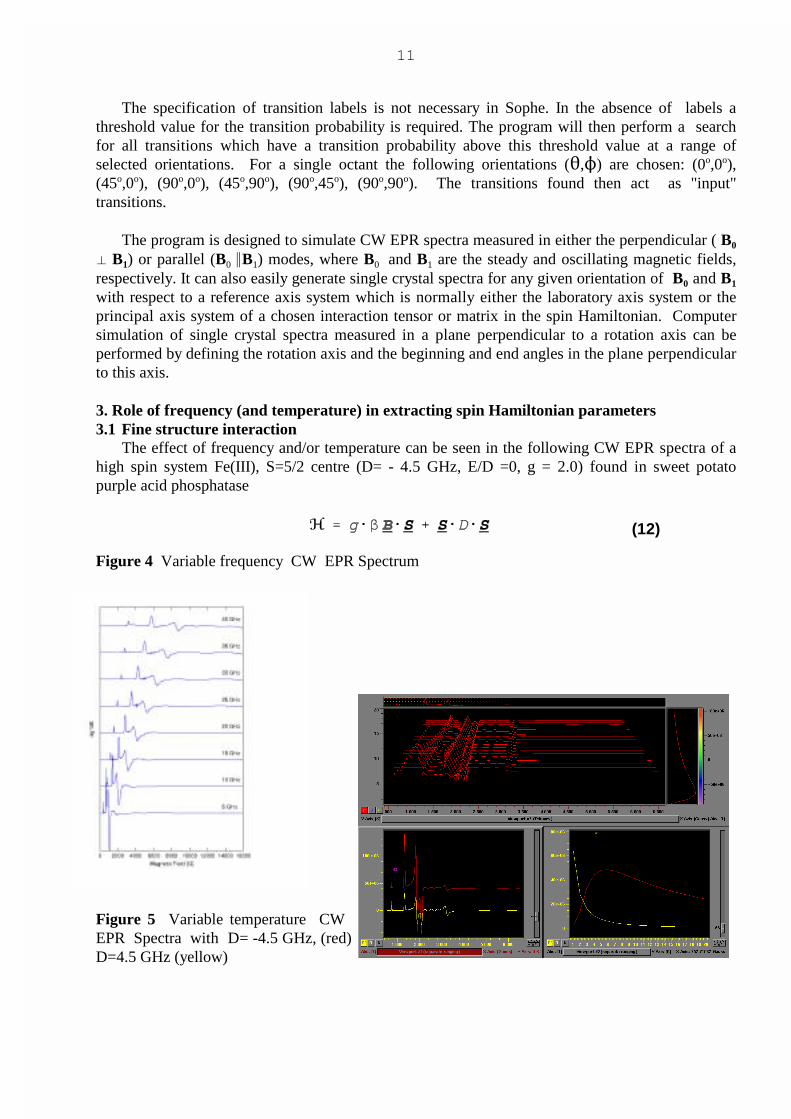
3. Role of frequency (and temperature) in extracting spin Hamiltonian parameters 3.1 Fine structure interaction

The effect of frequency and/or temperature can be seen in the following CW EPR spectra of ahigh spin system Fe(III), S=5/2 centre (D= - 4.5 GHz, E/D =0, g = 2.0) found in sweet potatopurple acid phosphatase

Figure 4 Variable frequency CW EPR Spectrum

Figure 5 Variable temperature CW EPR Spectra with D= -4.5 GHz, (red)D=4.5 GHz (yellow)

12

(13)

Conclusions Concerning Choice of Microwave Frequency� At very low frequencies (� < D) there is insufficient energy to observe all transitions.� Variable temperature experiments can be used to determine the magnitude and sign of the axial

zero field splitting, D.

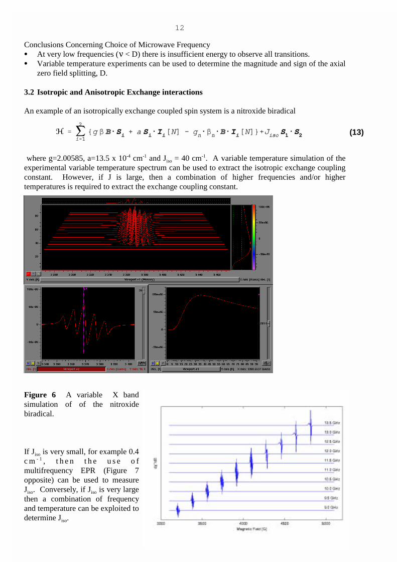
3.2 Isotropic and Anisotropic Exchange interactions

An example of an isotropically exchange coupled spin system is a nitroxide biradical

where g=2.00585, a=13.5 x 10-4 cm-1 and Jiso = 40 cm-1. A variable temperature simulation of theexperimental variable temperature spectrum can be used to extract the isotropic exchange couplingconstant. However, if J is large, then a combination of higher frequencies and/or highertemperatures is required to extract the exchange coupling constant.

Figure 6 A variable X bandsimulation of of the nitroxidebiradical.

If Jiso is very small, for example 0.4c m - 1 , t h e n t h e u s e o fmultifrequency EPR (Figure 7opposite) can be used to measureJiso. Conversely, if Jiso is very largethen a combination of frequencyand temperature can be exploited todetermine Jiso.

13

(14)

(16)

(15)

3.3 Distributions of parameters 3.3.1 Distributions of g and A values - Examples - Low Spin Fe(III) and Co(II) Centres

Distributions of g values results in better spectral resolution at lower frequencies.

For example a low spin Fe(III) S=1/2, I=0 spin system,gx=2.4, gy=,2.0 and gz=1.5

Figure 8 Multifrequency EPR Simulation of a low spinFe(III) spin system

Distributions of parameters (g and A values) can result in better spectra resolution at differentfrequencies

For example a low spin Co(II) with pyridine coordinated axially

Figure 9 Co(II) S=1/2, I=7/2, g�=1.972, g�=2.180,A�=77.5,x 10-4 cm-1 , A�= 47.8 x 10-4 cm-1,�R�=16.5 MHz, �R�=, 15.0 Mhz, �g�/g�=0.0016,�g�/g�=0.0034, �A�=,5.8, MHz �A�=,16.6 MHz.(a) X-band (9.5962 GHz) EPR Spectrum (red), (b)S-band (2.3 Ghz) CW EPR Spectrum (blue).

14

Conclusions Concerning Choice of Microwave Frequency� For spin systems with no hyperfine coupling, the lower the frequency, the narrower the

linewidth� For spin systems which contain nuclei, the optimum frequency for the best resolution of a given

hyperfine resonance depends upon a quadratic in MI and the frequency. Generally lowerfrequencies (L to S-band are better).

3.3.2 Distributions of D and E values

An example of a spin system which exhibits a distribution of D and E values is the EPR spectrum ofthe high spin Fe(III) (S=5/2) centres (~10%) in the sweet potato purple acid phosphatase enzymewhich contains a strongly antiferromagnetrically coupled binuclear Fe(III) -O-Mn(II) active site.

Figure 10 (a) CW EPR Spectrum of the Fe(III)-apoand Fe(III)-Zn(II) centres in sweet potato purple acidphosphatase. Experimental (red) and computersimulated (green) spectra. (c) CW EPR spectrum asa function of E/D and (d) a transition surface wherethe colour map (decreasing from red to blue)corresponds to the distribution of E/D.

15

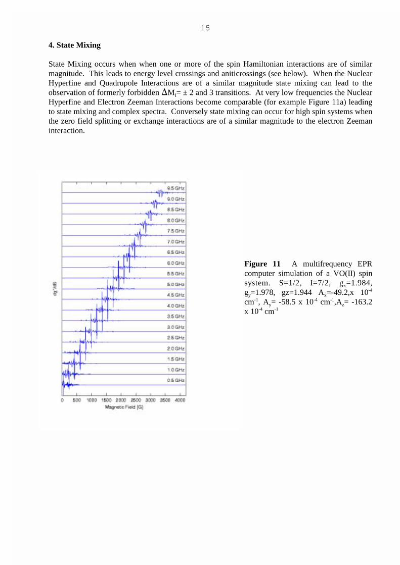
4. State Mixing

State Mixing occurs when when one or more of the spin Hamiltonian interactions are of similarmagnitude. This leads to energy level crossings and aniticrossings (see below). When the NuclearHyperfine and Quadrupole Interactions are of a similar magnitude state mixing can lead to theobservation of formerly forbidden �MI= ± 2 and 3 transitions. At very low frequencies the NuclearHyperfine and Electron Zeeman Interactions become comparable (for example Figure 11a) leadingto state mixing and complex spectra. Conversely state mixing can occur for high spin systems whenthe zero field splitting or exchange interactions are of a similar magnitude to the electron Zeemaninteraction.

Figure 11 A multifrequency EPRcomputer simulation of a VO(II) spinsystem. S=1/2, I=7/2, gx=1.984,gy=1.978, gz=1.944 Ax=-49.2,x 10-4

cm-1, Ay= -58.5 x 10-4 cm-1,Az= -163.2x 10-4 cm-1

16

(17)

3.3.3 Energy level crossings and anticrossings and looping transitions

These affects are commonly observed in CW EPR spectra of high spin systems, for example Fe(III),S=5/2, D= - 4.5 GHz, E/D =0, g = 2.0

Figure 12 (a) S-band, 4.0 GHz, (b) X-band, 9.75 GHz,

(c) Q-band, 35.0 GHz, (d) W-band, 95.0 GHz

Conclusions Concerning Choice of Microwave Frequency� CW EPR Spectra are simplified at higher frequencies� At very low frequencies (� < D) there is insufficient energy to observe all transitions

17

(18)

(19)

4. Role of frequency in spectral resolution

Two examples include Mo(V) and Cu(II) dimer spectra.

Figure 13 Multifrequency CW EPR spectra of [MoO(SPh)4]-.

(a,b) Solution spectra and (c,d) frozen solution spectra.

The parameters a, b, c and d are dependent on the themicrowave frequency, the hydrodynamic radius, the solventviscosity, temperature and the anisotropy of the g and Amatrices.

The narrower linewidths at lower microwave allow theobservation of superhyperfine interactions [47] and redistributesthe Mo hyperfine resonances providing a simpler interpretation.

The microwave frequency can be varied to separate multicomponent spectra. For exampleseparation of two S=1/2 spin systems can be achieved by using higher frequencies. Another use ofhigh frequencies is the separation of spectra from S=1/2 Cu(II) complexes from S=1 dipole-dipolecoupled spectra, the latter being frequency independent.

5. SummaryIn conclusion I hope I have demonstrated that a multifrequency approach in conjunction with

computer simulation allows the accurate determination of spin Hamiltonian parameters which canbe used to obtain structural information.

6. AcknowledgementsI would like to thank the Australian Research Council and the EPR Division of Bruker Analytik

for financial support and present and past members of the Sophe group, including Dr.ChristopherNoble, Dr. Kevin Gates, Dr. Anthyony Mitchell, Simon Benson, Mark Griffin, Andrae Muys, Dr.Demin Wang and Markus Heichel.

18

7. Bibliography[1] J. R. Pilbrow, “Transition Ion Electron Paramagnetic Resonance”, Clarendon Press, Oxford,

(1990).[2] F. E. Mabbs and D. C. Collison, “Electron Paramagnetic Resonance of Transition Metal

Compounds”, Elsevier, Amsterdam, (1992).[3] R. Basosi, W.E. Antholine, J.S. Hyde, “Multifrequency ESR of Copper Biophysical

Applications” in “Biological Magnetic Resonance” (L.J. Berliner, J. Reuben Eds.) Vol. 13,New York, Plenum Press, (1993).

[4] G.R. Hanson, A.A. Brunette, A.C. McDonell, K.S. Murray, and A.G. Wedd, J. Amer.Chem. Soc., 103, (1981) 1953.

[5] Y.S. Lebedev, Appl. Magn. Reson., 7, (1994) 339.[6] L.C. Brunel, Appl. Magn. Reson., 11, (1996) 417.[7] E.J. Reijerse, P.J. vanDam, A.A.K. Klaassen, W.R. Hagen, P.J.M. vanBentum, G.M. Smith,

Appl. Magn. Reson., 14, (1998) 153.[8] Abragam, A., Bleaney, B.,: Electron Paramagnetic Resonance of Transition Ions. Clarendon

Press, Oxford (1970).[9] A. Bencini and D. Gatteschi, “EPR of Exchange Coupled Systems”, Springer-Verlag,

Berlin, (1990).[10] T. D. Smith and J. R. Pilbrow, Coord. Chem. Rev., 13, (1974) 173.[11] P. C. Taylor, J. F. Baugher and H. M. Kriz, Chem. Rev., 75, (1975) 203.[12] (a) J. D. Swalen and H. M. Gladney, IBM J. Res. Dev., 8, (1964) 515.

(b) J. D. Swalen, T. R. L. Lusebrink and D. Ziessow, Magn. Reson. Rev., 2, (1973) 165.[13] H. L. Vancamp and A. H. Heiss, Magn. Reson. Rev., 7, (1981) 1.[14] B.J. Gaffney, H.J. Silverstone, “Simulation of the EMR Spectra of the High-Spin iron in

proteins” in “Biological Magnetic Resonance”, (L.J. Berliner, J. Reuben Eds.) Vol. 13, NewYork, Plenum Press, (1993).

[15] S. Brumby, J. Magn. Reson., 39, (1980) 1, ibid 40, (1980) 157.[16] D. Wang, G.R. Hanson, J. Magn. Reson. A, 117, (1995) 1.[17] D. Wang, G.R. Hanson, Appl. Magn. Reson., 11, (1996) 401.[18] K.E. Gates, M. Griffin, G.R. Hanson, K. Burrage, J. Magn. Reson., 135, (1998) 104.[19] (a) R. L. Belford and M. J. Nilges, EPR Symposium 21st Rocky Mountain Conference,

Denver, Colorado, (1979). (b) A. M. Maurice. PhD thesis, University of Illinois, Urbana, Illinois, (1980). (c ) M. J. Nilges, “Electron Paramagnetic Resonance Studies of Low Symmetry Nickel(I)and Molybdenum(V) Complexes”, PhD thesis, University of Illinois, Urbana, Illinois,(1979).

[20] M. C. M. Gribnau, J. L. C. van Tits, E. J. Reijerse, J. Magn. Reson., 90, (1990) 474.[21] A.Kretter, J. Huttermann, J. Magn. Reson. 93, (1991) 12.[22] J. R. Pilbrow, J. Magn. Reson., 58, (1984) 186.[23] E. Anderson, Z. Bai, C. Bischof, J. Demmel, J. Dongarra, J. Du Croz, A. Greenbaum, S.

Hammarling, A. McKenney, S. Ostrouchov, and D. Sorensen, “LAPACK Users' Guide”,SIAM, Philadelphia, (1992).

[24] D. W. Alderman, M. S. Solum and D. M. Grant, J. Chem. Phys., 84, (1986) 3717.[25] M. J. Mombourquette and J. A. Weil, “Simulation of Magnetic Resonance Powder Spectra.

J. Magn. Reson., 99, (1992) 37.[26] G. van Veen, J. Magn. Reson., 38, (1978) 91. [27] B.-Q. Su, D.-Y. Liu, “Computational geometry - Curves and Surface Modelling”, Academic

Press, Singapore, (1989).[28] D. Nettar, N.I. Villafranca, J. Magn. Reson., 64, (1985) 61.[29] M.I. Scullane, L.K. White, N.D. Chasteen, J. Magn. Reson., 47, (1982) 383.[30] D.G. McGavin, M.J. Mombourquette, J.A. Weil, “EPR ENDOR User’s manual”,

19

University of Saskatchewan, Saskatchewan, Canada, (1993).[31] G.G. Belford, R.L. Belford, J.F. Burkhalter, J. Magn. Reson., 11, (1973) 251.[32] T. Y. Li and N. H. Rhee, Numer. Math., 55, (1989) 265.[33] M. Oettli, Technical Report 205, Department Informatik, ETH, Zürich, Dec. (1993). and

references therein.[34] S. K. Misra, P. Vasilopoulos, J. Phys. C: Solid St. Phys., 13, (1980) 1083.[35] G. H. Golub, C. F. Van Loan, Matrix Computations. Johns Hopkins University Press,

Baltimore, Maryland, (1983).[36] (a) D. Kivelson, J. Chem. Phys. 33, (1960) 1094.

(b) R. Wilson, D. Kivelson, J. Chem. Phys. 44, (1966) 154, ibid 44, (1966) 4440.(c) P.W. Atkins, D. Kivelson, J. Chem. Phys. 44, (1966) 169.

[37] (a) W. Froncisz, J.S. Hyde, J. Chem. Phys. 73, (1980) 3123. (b) J.S. Hyde, W. Froncisz, Ann. Rev. Biophys. Bioeng. 11, (1982) 391.[38] R.F. Wenzel, Y.W. Kim, Phys. Rev. 140, (1965) 1592.[39] (a) G. R. Sinclair, “Modelling Strain Broadened EPR Spectra”, PhD thesis, Monash

University, (1988).(b) J.R. Pilbrow, G.R. Sinclair, D.R. Hutton, G.J. Troup, J. Mag. Reson., 52, (1983) 386.

[40] (a) S.K. Misra, J. Mag. Reson., 23, (1976) 403.(b) S.K. Misra, Mag. Reson. Rev., 10, (1986) 285.(c) S.K. Misra, Physica, 121B, (1983) 193.(d) S.K. Misra, S. Subramanian, J. Physics C, 15, (1982) 7199.

[41] Spin Hamiltonian parameters are constrained to a portion of �P-space as this will preventthe generation of a NULL spectrum.

[42] R. Hooke, T.A. Jeeves, J. Assoc. Computing Machinery, 8, (1961) 212.[43] W. Spendley, G.R. Hext, F.R. Himsworth, Technometrics, 4, (1962) 441.[44] (a) D.M. Nicholson, A. Chowdhary, L. Schwartz, Physical Review B, 29, (1984) 1633.

(b) I.O. Bohachevsky, M.E. Johnson, L.S. Myron, Technometrics, 28, (1986) 209.(c) A. Corana, M. Marchesi, C. Martini, S. Ridella, ACM Trans. Math. Software, 13, (1987)262.(d) H. Heynderickx, H. De Raedt, D. Schoemaker, J. Magn. Reson., 70, (1986) 134.

[45] R. Basosi, G. Della Lunga, R. Pogni, Appl. Magn. Reson., 11, (1996) 437.[46] Griffin, M.; Muys, A.; Noble, C.; Wang, D.; Eldershaw, C.; Gates, K.E.; Burrage, K.;

Hanson, G.R. XSophe, a Computer Simulation Software Suite for the Analysis of ElectronParamagnetic Resonance Spectra , 1999, Mol. Phys. Rep., 26, 60-84.

[47] Hanson, G.R.; Wilson, G.R.; Bailey, T.D.; Pilbrow, J.R.; Wedd, A.G. "Multifrequency ESRStudies of Molybdenum (V) and Tungsten (V) Compounds", J. Amer. Chem. Soc., 109,(1987) 2609.

[48] Heichel, M.; Höfer, P.; Kamlowski, A.; Griffin, M.; Muys, A.; Noble, C.; Wang, D.;Hanson, G.R.; Eldershaw, C.; Gates, K.E.; Burrage, K. Xsophe-Sophe-XeprView Bruker'sprofessional CW-EPR Simulation Suite, Bruker Report, 148, (2000) 6-9.