Precision requirements for space-based XCO2 data
58
Precision requirements for space-based X CO2 data 1 2 3 4 5 6 7 8 9 10 11 12 13 14 15 16 17 18 19 20 21 22 23 24 25 26 27 28 29 30 31 32 33 34 35 36 37 38 39 40 41 42 C. E. Miller 1 , D. Crisp 1 , P. L. DeCola 2 , S. C. Olsen 3 , J. T. Randerson 4 , A. Michalak 5 , A. Alkhaled 6 , P. Rayner 7 , D. J. Jacob 8 , P. Suntharalingam 8 , D. Jones 9 , A. S. Denning 10 , M. E. Nicholls 10 , S. C. Doney 11 , S. Pawson 12 , H. Boesch 1 , B. J. Connor 13 , I. Y. Fung 14 , D. O’Brien 10 , R. J. Salawitch 1 , S. P. Sander 1 , B. Sen 1 , P. Tans 15 , G. C. Toon 1 , P. O. Wennberg 16 , S. C. Wofsy 8 , Y. L. Yung 16 1 Jet Propulsion Laboratory, California Institute of Technology, Pasadena, California USA 2 NASA Headquarters, Washington, DC USA 3 Los Alamos National Laboratory, Los Alamos, New Mexico USA 4 Department of Earth System Science, University of California, Irvine, California USA 5 Department of Civil and Environmental Engineering and Department of Atmospheric, Oceanic and Space Sciences, The University of Michigan, Ann Arbor, Michigan USA 6 Department of Civil and Environmental Engineering, The University of Michigan, Ann Arbor, Michigan USA 7 Laboratoire des Sciences du Climat et de l'Environnement/IPSL, CEA-CNRS-UVSQ, Gif-sur- Yvette, France 8 Division of Engineering and Applied Science and Department of Earth & Planetary Sciences, Harvard University, Cambridge, Massachusetts USA 9 Department of Physics, University of Toronto, Toronto, Ontario, Canada 10 Atmospheric Science Department, Colorado State University, Fort Collins, Colorado USA 11 Woods Hole Oceanographic Institution, Woods Hole, Massachusetts USA 12 Goddard Earth Science and Technology Center, Baltimore, Maryland, USA and Global Modeling and Assimilation Office, NASA Goddard Space Flight Center, Greenbelt, Maryland USA. 13 National Institute of Water and Atmospheric Research, Omakau, Central Otago, New Zealand 14 Berkeley Atmospheric Sciences Center, University of California, Berkeley, Berkeley, California USA 15 NOAA Climate Monitoring and Diagnostics Laboratory, Boulder, Colorado USA 16 Division of Geological and Planetary Sciences, California Institute of Technology, Pasadena, California USA Corresponding Author: Charles Miller MS 183-501 Jet Propulsion Laboratory 4800 Oak Grove Drive Pasadena, CA 91109-8099 Tel: 818.393.6294 Fax: 818.354.0966 [email protected] 43 44 6/12/2006 7:14 PM
Transcript of Precision requirements for space-based XCO2 data
Precision requirements for space-based XCO2 data 123456789
101112131415161718192021222324252627282930313233343536373839404142
C. E. Miller1, D. Crisp1, P. L. DeCola2, S. C. Olsen3, J. T. Randerson4, A. Michalak5, A. Alkhaled6, P. Rayner7, D. J. Jacob8, P. Suntharalingam8, D. Jones9, A. S. Denning10, M. E. Nicholls10, S. C. Doney11, S. Pawson12, H. Boesch1, B. J. Connor13, I. Y. Fung14, D. O’Brien10,R. J. Salawitch1, S. P. Sander1, B. Sen1, P. Tans15, G. C. Toon1, P. O. Wennberg16, S. C. Wofsy8,Y. L. Yung16
1Jet Propulsion Laboratory, California Institute of Technology, Pasadena, California USA2NASA Headquarters, Washington, DC USA 3Los Alamos National Laboratory, Los Alamos, New Mexico USA 4Department of Earth System Science, University of California, Irvine, California USA5Department of Civil and Environmental Engineering and Department of Atmospheric, Oceanic and Space Sciences, The University of Michigan, Ann Arbor, Michigan USA6Department of Civil and Environmental Engineering, The University of Michigan, Ann Arbor, Michigan USA7Laboratoire des Sciences du Climat et de l'Environnement/IPSL, CEA-CNRS-UVSQ, Gif-sur-Yvette, France8Division of Engineering and Applied Science and Department of Earth & Planetary Sciences, Harvard University, Cambridge, Massachusetts USA9Department of Physics, University of Toronto, Toronto, Ontario, Canada 10Atmospheric Science Department, Colorado State University, Fort Collins, Colorado USA 11Woods Hole Oceanographic Institution, Woods Hole, Massachusetts USA 12Goddard Earth Science and Technology Center, Baltimore, Maryland, USA and Global Modeling and Assimilation Office, NASA Goddard Space Flight Center, Greenbelt, Maryland USA.13National Institute of Water and Atmospheric Research, Omakau, Central Otago, New Zealand 14Berkeley Atmospheric Sciences Center, University of California, Berkeley, Berkeley, California USA15NOAA Climate Monitoring and Diagnostics Laboratory, Boulder, Colorado USA 16Division of Geological and Planetary Sciences, California Institute of Technology, Pasadena, California USA
Corresponding Author: Charles Miller MS 183-501 Jet Propulsion Laboratory 4800 Oak Grove Drive Pasadena, CA 91109-8099 Tel: 818.393.6294 Fax: 818.354.0966 [email protected]
44
6/12/2006 7:14 PM

MILLER ET AL.: PRECISION REQUIREMENTS FOR SPACE-BASED XCO2
Abstract454647
48
49
50
51
52
53
Precision requirements are determined for space-based column-averaged CO2 dry air mole
fraction (XCO2) data. These requirements result from an assessment of spatial and temporal
gradients in XCO2, the relationship between XCO2 precision and surface CO2 flux uncertainties
inferred from inversions of the XCO2 data, and the effects of XCO2 biases on the fidelity of CO2
flux inversions. Observational system simulation experiments and synthesis inversion modeling
demonstrate that the Orbiting Carbon Observatory (OCO) mission design and sampling strategy
provide the means to achieve these XCO2 data precision requirements.
Monday, June 12, 2006 7:14 PM 2
MILLER ET AL.: PRECISION REQUIREMENTS FOR SPACE-BASED XCO2
54
55
56
57
58
59
60
61
62
63
64
65
66
67
68
69
70
71
72
73
74
75
76
1 Introduction
Carbon dioxide (CO2) is a natural component of the Earth’s atmosphere and a strong greenhouse
forcing agent. Concentrations of atmospheric CO2 fluctuated between 185 and 300 parts per
million (ppm) over the last 500,000 years [IPCC, 2001]. However, since the dawn of the
industrial era 150 years ago, human activity (fossil fuel combustion, land use change, etc.) has
driven atmospheric CO2 concentrations from 280 ppm to greater than 375 ppm. Such a dramatic
short-term increase in atmospheric CO2 is unprecedented in the recent geologic record,
prompting Crutzen to label the current era as the Anthropocene [Crutzen, 2002]. Better carbon
cycle monitoring capabilities and insight on the underlying dynamics controlling atmosphere
exchange with the land and ocean reservoirs are needed as society begins to discuss active
management of the global carbon system [Dilling et al., 2003].
Data from the existing network of surface in situ CO2 measurement stations [GLOBALVIEW-
CO2, 2005] indicate that the terrestrial biosphere and oceans have absorbed almost half of the
anthropogenic CO2 emitted during the past 40 years. The nature, geographic distribution and
temporal variability of these CO2 sinks are not adequately understood, precluding accurate
predictions of their responses to future climate change [Friedlingstein et al., 2006; Cox et al.,
2000; Fung et al., 2005]. Inverse modeling of the surface in situ CO2 data [GLOBALVIEW-CO2,
2005] provide compelling evidence for a Northern Hemisphere terrestrial carbon sink, but the
network is too sparse to quantify the distribution of the sink over the North American and
Eurasian biospheres or to estimate fluxes over the Southern Ocean [Gurney et al., 2005; Gurney
et al., 2002; Gurney et al., 2003; Gurney et al., 2004; Law et al., 2003; Baker et al., 2006a].
Monday, June 12, 2006 7:14 PM 3

MILLER ET AL.: PRECISION REQUIREMENTS FOR SPACE-BASED XCO2
77
78
79
80
81
82
83
84
85
86
87
88
89
90
91
92
93
94
95
96
97
98
99
Existing models and measurements also have difficulty explaining why the atmospheric CO2
accumulation varies from 1 to 7 gigatons of carbon (GtC) per year in response to steadily
increasing emission rates.
Space-based remote sensing of atmospheric CO2 has the potential to deliver the data needed to
resolve many of the uncertainties in the spatial and temporal variability of carbon sources and
sinks. Several sensitivity studies have evaluated the improvement in carbon flux inversions that
would be provided by precise, global space-based column CO2 data [Dufour and Breon, 2003;
Houweling et al., 2004; Mao and Kawa, 2004; O'Brien and Rayner, 2002; Rayner et al., 2002;
Rayner and O'Brien, 2001; Baker et al., 2006b]. The consensus of these studies is that satellite
measurements yielding the column-averaged CO2 dry air mole fraction, XCO2, with bias-free
precisions in the range of 1 – 10 ppm (0.3 – 3.0%) will reduce uncertainties in CO2 sources and
sinks due to uniform and dense global sampling. As Houweling et al. [Houweling et al., 2004]
demonstrated, the precision requirements for space-based XCO2 data vary depending on the
spatial and temporal resolution of the data and the spatiotemporal scale of the surface flux
inversion. Clearly, the highest precision XCO2 data (e.g. 1 ppm or better) would best address the
largest number of carbon cycle science questions. However, this requirement must be balanced
against the significant technical challenges of delivering a satellite
measurement/retrieval/validation system that can produce bias-free, sub-1% precision XCO2 data.
The space-based XCO2 data must also be accurately calibrated to the WMO reference scale for
atmospheric CO2 measurements so that they can be ingested simultaneously with sub-orbital data
in synthesis inversion or data assimilation schemes without producing spurious fluxes.
Monday, June 12, 2006 7:14 PM 4
MILLER ET AL.: PRECISION REQUIREMENTS FOR SPACE-BASED XCO2
The Orbiting Carbon Observatory (OCO) was selected by NASA’s Earth System Science
Pathfinder (ESSP) program in July 2002 to deliver space-based X
100
101
102
103
104
105
106
107
108
109
110
111
112
113
114
115
116
117
118
119
120
121
CO2 data products with the
precision, temporal and spatial resolution, and coverage needed to quantify CO2 sources and
sinks on regional spatial scales and characterize their variability on seasonal to interannual time
scales [Crisp et al., 2004]. The mission is designed for a two-year operational period with launch
scheduled for 2008, the first year of the Kyoto Protocol commitment period. OCO will join the
EOS Afternoon Constellation (A-Train), flying in a sun-synchronous polar orbit with a constant
1:26 PM local solar time (1326 LST) flyover, a 16-day (233 orbit) repeat cycle and near global
sampling.
The OCO science team analyzed a broad range of measurement and modeling data to define the
science requirements for space-based XCO2 data precision. The products of this investigation
address two fundamental questions:
1. What precision does the OCO XCO2 data product need to improve our understanding of CO2
surface fluxes (sources and sinks) significantly?
2. Does the measurement/retrieval/validation approach adopted in the OCO mission design
provide the needed XCO2 data precision?
This paper analyzes atmospheric CO2 observations and modeling studies of CO2 sources and
sinks to derive the science requirements for space-based XCO2 data precision (Question 1).
Analyses of space-based and sub-orbital measurements, as well as the development and
validation of retrieval algorithms demonstrating the potential of the OCO mission design to
Monday, June 12, 2006 7:14 PM 5

MILLER ET AL.: PRECISION REQUIREMENTS FOR SPACE-BASED XCO2
achieve the required XCO2 precision (Question 2) are the subject of recent [Kuang et al., 2002;
Boesch et al., 2006; Washenfelder et al., 2006] and ongoing studies.
122
123
124
125
126
127
128
129
130
131
132
133
134
135
136
137
138
139
140
141
142
143
144
2 XCO2 Precision Requirements
Two community-wide undertakings define the current state of knowledge for the atmospheric
CO2 budget: the GLOBALVIEW-CO2 in situ measurement network [GLOBALVIEW-CO2, 2005]
and the TransCom 3 transport/flux estimation experiment [Gurney et al., 2005; Gurney et al.,
2002; Gurney et al., 2003; Gurney et al., 2004; Law et al., 2003; Baker et al., 2006a]. The
GLOBALVIEW-CO2 network’s emphasis on acquiring accurate measurements through rigorous
experimental methods, constant calibration using procedures and materials traceable to WMO
standards, and continual vigilance against biases has created the recognized reference standard
data set for atmospheric CO2 observations. The network collects surface in situ CO2
measurements at approximately 120 stations worldwide, spanning latitudes from the South Pole
to 82.4°N (Alert, Canada). Typical measurement uncertainties are on the order of 0.1 ppm
(0.03%).
The TransCom 3 project [Gurney et al., 2005; Gurney et al., 2002; Gurney et al., 2003; Gurney
et al., 2004; Law et al., 2003; Baker et al., 2006a] reported estimates of carbon sources and sinks
from variations in the GLOBALVIEW-CO2 data via inverse modeling with atmospheric
transport models. This assessment found that carbon fluxes integrated over latitudinal zones are
strongly constrained by observations in the middle to high latitudes. Flux uncertainties were also
constrained by inadequacies in the transport models and the lack of observations in the tropics.
The latter result is not surprising since the GLOBALVIEW-CO2 network strategy was originally
Monday, June 12, 2006 7:14 PM 6
MILLER ET AL.: PRECISION REQUIREMENTS FOR SPACE-BASED XCO2
designed specifically to avoid measurement contamination from air locally influenced by large
CO
145
146
147
148
149
150
151
152
153
154
155
156
157
158
159
160
161
162
163
164
165
166
167
2 sources or sinks. The inversions also exhibited significant uncertainties when trying to
distinguish meridonal contributions to the fluxes.
Rayner and O’Brien [2001] showed that space-based XCO2 data could dramatically improve our
understanding of CO2 sources and sinks if these measurements provided adequate precision and
spatial coverage. This study used a synthesis inversion model to estimate the surface-atmosphere
CO2 flux uncertainties in 26 continent/ocean basin scale regions. The baseline was established
by using measurements from 56 stations in the ground-based GLOBALVIEW-CO2 network.
The results were compared to simulations that used spatially-resolved, global XCO2 data. Rayner
and O’Brien found that global, space-based XCO2 data with 2.5 ppm precisions (and no biases) on
8o × 10o scales would be needed to match the performance of the existing ground based network.
Space-based XCO2 data with 1 ppm precisions were predicted to reduce inferred CO2 flux
uncertainties from greater than 1.2 GtC region 1 year 1 to less than 0.5 GtC region 1 year 1 when
averaged over the annual cycle. Additionally, the uncertainties in all regions were more uniform
for inversions using the space-based XCO2 data.
While these simulations clearly illustrate the advantages of precise space-based XCO2 data, they
do not explicitly quantify the data precision required for OCO, because they do not simulate the
spatial and temporal sampling strategy proposed for the OCO mission. Nor do they adequately
characterize the sensitivity of source-sink inversions to XCO2 data precision. To address these
concerns, we combined available atmospheric CO2 data and transport models to estimate XCO2
spatial gradients as well as global and regional scale XCO2 variability. A series of Observational
Monday, June 12, 2006 7:14 PM 7

MILLER ET AL.: PRECISION REQUIREMENTS FOR SPACE-BASED XCO2
System Simulation Experiments (OSSE’s) sampled the synthetic CO2 fields using strategies
simulating the GLOBALVIEW-CO
168
169
170
171
172
173
174
175
176
177
178
179
180
181
182
183
184
185
186
187
188
189
2 surface network [GLOBALVIEW-CO2, 2005] as well as the
OCO satellite. Inverse modeling of these data characterized the relationship between the inferred
surface flux uncertainties and uncertainties in the space-based XCO2 data. We also investigated
the use of inversions to detect bias in the XCO2 data and what level of sensitivity such analyses
would provide.
2.1 XCO2 Spatial and Temporal Gradients
Distributions of atmospheric CO2 were simulated with the Model of Atmospheric Transport and
Chemistry (MATCH) three-dimensional atmospheric transport model [Olsen and Randerson,
2004]. MATCH represents advective transport using a combination of horizontal and vertical
winds and has parameterizations of wet and dry convection and boundary layer turbulent mixing
[Rasch et al., 1994]. MATCH operates off-line using archived meteorological fields which for
this study were derived from the NCAR Community Climate Model version 3 with T21
horizontal resolution (approximately 5.5° × 5.5°) and 26 vertical levels from the surface up to 0.2
hPa (about 60 km) on hybrid sigma pressure levels. The top of the first model level is
approximately 110 m. The meteorological fields represent a climatologically ‘‘average’’ year
rather than any specific year. This meteorological data was archived every 3 model hours and
was interpolated to the 30-min MATCH time step. In this configuration MATCH has an
interhemispheric transport time of approximately 0.74 years, about in the middle of the 0.55 year
to 1.05 year range of the models that participated in the TransCom 2 experiment [Denning et al.,
1999]. A single year of dynamical inputs was recycled for the multiyear runs used in this study.
Monday, June 12, 2006 7:14 PM 8

MILLER ET AL.: PRECISION REQUIREMENTS FOR SPACE-BASED XCO2
Constraints on CO2 sources and sinks incorporated fossil fuel emissions as estimated by Andres
et al. [Andres et al., 1996], atmosphere-oceanic exchange as estimated from sea-surface pCO2
measurement by Takahashi et al. [Takahashi et al., 2002], and biospheric fluxes modeled using
the Carnegie-Ames-Stanford Approach (CASA) model [Randerson et al., 1997], including a
diurnal cycle of photosynthesis and respiration. These fluxes were transported using MATCH for
the year 2000 [Olsen and Randerson, 2004]. Simulated X
190
191
192
193
194
195
196
197
198
199
200
201
202
203
204
205
206
207
208
209
210
211
212
213
CO2 data were subsampled from the
model output by integrating vertically according to the OCO averaging kernel.. In these
simulations terrestrial ecosystem exchange was annually balanced; in other words, we omitted a
‘‘missing’’ carbon sink necessary to balance fossil carbon sources with the atmospheric CO2
growth rate [Gurney et al., 2002; Tans et al., 1990].
The 15th of each month was taken as a proxy for the monthly mean. Data were extracted for 1300
local time globally, as a preliminary approximation of XCO2 as would be observed by OCO. The
resulting data are presented for January and July 2000 in Figure 1. These data differ slightly from
the monthly mean XCO2 maps presented in Figure 9 of [Olsen and Randerson, 2004], capturing
more of the instantaneous XCO2 variability. All model values are reported relative to the annual
mean surface mixing ratio south of 60° South. Figure 1 shows that the Northern Hemisphere
XCO2 variability is typically about 6 ppm. This is only 50% of the amplitude of the seasonal cycle
in the near-surface concentrations of CO2 (see Figure 5 of Olsen and Randerson [2004]).
Somewhat larger high frequency variations, associated with passing weather systems and strong
source regions, are also common. The monthly peak-to-peak amplitude of Southern Hemisphere
XCO2 is typically 2-3 ppm while the annual peak-to-peak amplitude varies from 6-7 ppm over
tropical forests to less than 3 ppm over the Southern Ocean.
Monday, June 12, 2006 7:14 PM 9

MILLER ET AL.: PRECISION REQUIREMENTS FOR SPACE-BASED XCO2
These results indicate that space-based XCO2 data with precisions of 1 – 2 ppm are needed to
resolve the peak-to-peak amplitudes in monthly and annual X
214
215
216
217
218
219
220
221
222
223
224
225
226
CO2. This precision is also
sufficient to resolve regional scale meridional variations over the northern hemisphere boreal
forests or the Southern Ocean. The OCO sampling strategy (Section 4) is specifically designed
to return space-based measurements with the high sensitivity and dense sampling in space and
time required to attain this precision even when cloud and aerosol interference prevents
observations of the complete atmospheric column in the majority of the observed scenes.
2.2 Global and Regional XCO2 Variability
Global XCO2 spatial variability was quantified by analyzing the CASA/MATCH XCO2 data
calculated for 2000 [Olsen and Randerson, 2004]. Raw and experimental variograms were
calculated to quantify the global variability of XCO2. The raw variogram is defined for any two
measurements as [Cressie, 1991]
2'21
xzxzh227
228
229
230
231
(1)
where (h) is the raw variogram, z(x) is a measurement value at location x, z(x ) is a measurement
value at location x , and h is the separation distance between x and x’. In this case, the distance
was calculated using the great circle distance between points on the surface of the earth (e.g.
Michalak et al. 2004):
jijijiji rh coscoscossinsincos, 1xx (2) 232
where the coordinates iii ,x are the latitude and longitude, respectively, of the sample
locations, and r is the mean radius of the earth. The experimental variogram is a binned version
233
234
Monday, June 12, 2006 7:14 PM 10

MILLER ET AL.: PRECISION REQUIREMENTS FOR SPACE-BASED XCO2
of the raw variogram. The consistent North-South XCO2 gradient was accounted for by detrending
the data with respect to latitude. The resulting variograms are presented in Figure 2.
235
236
237
238
239
The experimental variogram for each month was fitted using an exponential theoretical
variogram model [Cressie, 1991; Michalak et al., 2004]
L
hh exp12 (3)240
241
242
243
244
245
246
247
248
249
250
251
252
253
254
255
256
257
Where 2 is the semivariance and L is the length parameter. The theoretical variogram describes
the decay in spatial correlation between pairs of XCO2 measurements as a function of physical
separation distance between these samples. The overall variance at large separation distances is
2 2 and the practical correlation range is approximately 3L. The 2 and L parameters were
estimated using a least-squares fit to the raw variogram. The fitted variograms are presented in
Figure 2, and the global variance and correlation range for each month are summarized in Table
1. The correlation length represents the distance at which the expected covariance between z(x)
and z(x ) approaches zero, and the measurement z(x ) no longer provides useful information about
the XCO2 value z(x). The variance indicates the maximum uncertainty at unsampled locations, in
the absence of nearby measurements, assuming the overall mean is known.
This analysis shows that the CASA/MATCH XCO2 field exhibits significant spatial correlation
and that the degree of spatial correlation varies throughout the year. The variance is higher
during the Northern Hemisphere summer and lower in winter. The seasonality of the global
correlation length is less pronounced, but follows a similar pattern to that of the sill. These two
factors have opposite effects on the required sampling intensity (i.e. a higher variance leads to a
larger number of required sampling locations whereas a longer correlation length reduces the
Monday, June 12, 2006 7:14 PM 11

MILLER ET AL.: PRECISION REQUIREMENTS FOR SPACE-BASED XCO2
number of required samples). Overall, because of the stronger seasonality of the variance of the
X
258
259
260
261
262
263
264
CO2 distribution, it is expected that a larger fraction of samples will need to be processed in
summer months in order to achieve a specified level of uncertainty in the interpolated XCO2 field.
Based on this global analysis, an average sampling interval of approximately 1500 km will be
required globally to achieve an interpolated XCO2 uncertainty with a standard deviation below 1
ppm. This estimate is based on:
2max
0 21ln
VLh (4)265
266
267
268
269
270
271
272
273
274
275
276
277
278
279
where L and 2 are taken from the theoretical variogram and Vmax is the maximum allowable
uncertainty, expressed as a variance. In the above calculation, we used the annual mean
parameters and Vmax = 1 ppm2. Note that this analysis assumes that either (i) the value sampled
by OCO is representative of the average XCO2 on the scale modeled by CASA/MATCH, or that
(ii) the covariance structure as estimated at the CASA/MATCH model grid scale is valid at the
smaller OCO measurement scale. In reality, OCO will measure at a significantly smaller scale
than the CASA/MATCH model resolution, and data at smaller scales tend to exhibit more
variability relative to measurements that represent averages at larger scales. For these reasons,
we expect the sampling interval required to achieve a maximum 1 ppm2 uncertainty in the
interpolated XCO2 product to be smaller for the OCO sampling scale relative to the
CASA/MATCH data. Note also that we have not considered measurement errors in this
calculation, which would again increase the amount of sampling required to constrain the
interpolated error to a given uncertainty threshold.
Monday, June 12, 2006 7:14 PM 12

MILLER ET AL.: PRECISION REQUIREMENTS FOR SPACE-BASED XCO2
To assess the regional variability of XCO2, a separate variogram was constructed for each grid cell
of the 5.5
280
281
282
283
284
285
286
287
288
289
290
291
292
293
294
295
296
297
298
299
300
301
302
o × 5.5o model output (2048 cells globally), centered at that grid cell. In calculating the
raw variogram for each grid cell, only pairs of data points with at least one member within a
2000 km radius of the grid cell were considered. Therefore, the raw variogram consisted of data
pairs where either (i) both measurements were within 2000 km of the central grid cell, or (ii) one
measurement was within 2000 km of the central grid cell and the other was not. In essence, this
approach quantifies the variability between measurements in the vicinity of a grid cell and the
global distribution.
The regional-scale raw variograms were fitted in a least-squares fashion using an exponential
variogram. The resulting correlation lengths and variances of the fitted theoretical variograms are
presented in Figures 3 and 4, respectively. These global maps of parameters describe the regional
correlation structure of the CASA/MATCH XCO2. The correlation structure exhibits temporal
variability, as was seen in Figure 2, as well as strong spatial variability. This can be observed
both in the variance and correlation lengths of the XCO2 distributions. For example, XCO2 in the
northern hemisphere is correlated over shorter distances than the global average (Figure 3).
The results of the regional XCO2 variability analysis are qualitatively consistent with the results of
Lin et al. [2004], who also found longer correlation lengths over the Pacific relative to
continental North America in their analysis of aircraft-dervied partial-XCO2 fields. A quantitative
comparison is difficult to establish because Lin et al. [2004] used a non-stationary power
variogram to represent CO2 variability. Such a variogram does not have a finite sill or
correlation length to compare to those presented in Figures 3 and 4. One quantitative
Monday, June 12, 2006 7:14 PM 13
MILLER ET AL.: PRECISION REQUIREMENTS FOR SPACE-BASED XCO2
comparison that can be made is a calculation of the separation distance at which the expected
difference in X
303
304
305
306
307
308
309
310
311
312
313
314
315
316
317
318
319
320
321
322
323
324
CO2 at two sampling locations is expected to reach a specified variance. Based on
the variogram used in Lin et al. [2004], the separation distance at which the squared difference
between vertically-integrated CO2 concentrations (< 9km) is expected to reach 1 ppm2 is 57 km
over the North American continent in June 2003, and 727 km over the Pacific Ocean. Data over
the Pacific Ocean were a composite of multiple years of springtime (February to April) and fall
(August to October) data. For the CASA/MATCH data, the separation distance is 290 km over
the North American continent for June 2000, and 3900 km (March 2000) and 790 km
(September 2000) over the Pacific Ocean. Overall, the variability over the Pacific Ocean is
comparable between the two datasets. The greater variability inferred over the North American
continent by Lin et al. [2004] is most likely largely due to the scale at which the aircraft
campaign measurements were taken relative to the scale of the CASA/MATCH modeled data.
As was previously discussed, data at finer scales typically exhibit more variability relative to
coarser data. This will need to be considered further in interpreting global model data in the
context of fine scale OCO measurements. Regional scale XCO2 variability will also be driven by
local conditions and meteorology [Nicholls et al., 2004]. Spatial and temporal heterogeneity of
the XCO2 covariance structure must therefore be taken into account in the design of a sampling
strategy and retrievals.
3 CO2 Fluxes from XCO2 Inversions
3.1 Relationship between OCO XCO2 Precision and Surface CO2 Flux Uncertainties
The synthesis inversion methods of Rayner and O’Brien [O'Brien and Rayner, 2002; Rayner et
Monday, June 12, 2006 7:14 PM 14
MILLER ET AL.: PRECISION REQUIREMENTS FOR SPACE-BASED XCO2
al., 2002; Rayner and O'Brien, 2001] were used to evaluate the impact of particular OCO
mission design choices and the resultant regional scale X
325
326
327
328
329
330
331
332
333
334
335
336
337
338
339
340
341
342
343
344
345
346
347
CO2 data precisions on the surface CO2
flux uncertainties inferred from synthesis inversion models. The OSSEs approximate the OCO
spatial and temporal sampling strategy to characterize the surface CO2 flux uncertainties for
different XCO2 data precisions. The spatial grid used in these experiments has higher spatial
resolution than that used by Rayner and O’Brien [Rayner and O'Brien, 2001] to assess more
accurately the distribution of flux uncertainties on regional scales [O'Brien and Rayner, 2002;
Rayner et al., 2002].
Following Rayner and O’Brien [Rayner and O'Brien, 2001], a baseline for comparisons with the
simulated space-based XCO2 data was established by performing synthesis inversion experiments
to estimate the CO2 flux uncertainties for the GLOBALVIEW-CO2 surface CO2 monitoring
network over the seasonal cycle. These flux errors are expressed in grams of carbon per square
meter per year, (gC m 2 yr 1). The prior uncertainty for all regions was assumed to be 2000 gC
m 2 yr 1. Results from simulations that employed weekly CO2 flask samples for 72 surface
stations are shown for January (Jan) and July (Jul) in Figure 5a-b. For this baseline case most
regions have flux uncertainties in excess of 1000 gC m 2 yr 1 with uncertainties greater than
1500 gC m 2 yr 1 typical for most land regions.
Figures 5c-d show the flux uncertainties inferred by inverting the baseline flask data augmented
by continuous surface measurements from 25 stations. Continuous surface measurements
produce their greatest benefits in the vicinity of measurement stations that are located well away
from strong sources and sinks. Even with the addition of the continuous CO2 measurements, flux
Monday, June 12, 2006 7:14 PM 15

MILLER ET AL.: PRECISION REQUIREMENTS FOR SPACE-BASED XCO2
uncertainties remain greater than 1000 gC m 2 yr 1 in most continental regions near strong
surface fluxes because of the limited spatial coverage offered by the continuous monitoring
stations. The largest uncertainties are seen in South America, central Africa, and southern Asia.
348
349
350
351
352
353
354
355
356
357
358
359
360
361
362
363
364
365
366
367
368
369
370
Figure 6 shows January (Jan) and July (Jul) CO2 flux uncertainties from synthesis inversion
simulations assuming XCO2 data sampled along the OCO orbit track with 1ppm (0.3%, Figure 6a-
b) and 5 ppm (1.5%, Figure 6c-d) precisions for monthly averages on 4o latitude 5o longitude
scales. For well-constrained regions in which the prior estimate has little impact, the flux
uncertainty increases from ~40 to ~200 gC m 2 yr 1 in the tropics and at mid-latitudes as the XCO2
data precision increases from 1 to 5 ppm. The relationship between XCO2 data precision and
surface flux uncertainties breaks down for regions smaller than 4o 5o (see Australia in Figs 5
and 6) and at high latitudes where the measurement frequency is lower. Such problems can be
reduced by calculating fluxes over larger spatial scales after performing the inversion.
The Northern Hemisphere terrestrial carbon sink is thought to absorb about 1 GtC yr 1 from the
atmosphere [Gurney et al., 2002]. The results presented in Figure 6 indicate that space-based
XCO2 data with monthly averaged precision of 1 – 2 ppm (0.3 to 0.5%) will yield flux
uncertainties no greater than ~100 gC m 2 yr 1 or 0.1 GtC (106 km2) 1 yr 1. Inversions using such
space-based XCO2 data should be able to detect the 1 GtC yr 1 carbon sink if it is confined to an
area or areas smaller than a few 1000 km × 1000 km regions, e.g. Northeastern North America.
We anticipate even greater sensitivity to detecting such a sink if space-based XCO2 and in situ
surface CO2 data are combined in the inversion.
Monday, June 12, 2006 7:14 PM 16

MILLER ET AL.: PRECISION REQUIREMENTS FOR SPACE-BASED XCO2
Comparisons of theflux uncertainties inferred from the 5 ppm precision XCO2 data (Figure 6c-d)
with results from the baseline inversion (Figure 5a-b) show that, even at this degraded precision,
the satellite data still provide a better constraint on surface fluxes for most regions. Augmenting
the surface network with continuous monitoring stations (Figure 5c-d) improves the surface flux
constraints for regions that contain one of these continuous monitoring sites, but still provides
inadequate constraints in other regions, particularly tropical forests. Because of uniform spatial
sampling over land and ocean and sheer data volume, space-based X
371
372
373
374
375
376
377
378
379
380
381
382
383
384
385
386
387
388
389
390
391
392
393
CO2 data will make a
substantial impact on reducing continental scale flux uncertainties even at 5 ppm precision.
3.2 Effects of Systematic XCO2 Bias on CO2 Flux Inversions
The precision requirements space-based XCO2 data presented in Section 2 assumed random errors
with no significant spatially- or temporally-coherent biases. This section addresses the potential
impact of systematic biases in the space-based XCO2 data on inferred CO2 flux uncertainties.
Systematic biases might result from such measurement considerations as signal to noise ratio,
viewing geometry, whether the observations were made over land or ocean, spatial variations in
clouds or aerosols, topographic variations, diurnal effects on the vertical CO2 profile, etc. The
effects of such biases on flux uncertainties depend on their spatial and temporal scale since CO2
sources and sinks are inferred from XCO2 gradients. Constant global biases do not compromise
XCO2-only flux inversions because they introduce no spurious gradients in the XCO2 fields that
could be misinterpreted as sources or sinks; however, a constant bias in space-based XCO2 data
would complicate inversions or assimilations that also included suborbital data or data from
other satellite platforms. Biases occurring on spatial scales smaller than ~30 km are not a major
concern because they will be indistinguishable from random noise contributions like scene-
Monday, June 12, 2006 7:14 PM 17

MILLER ET AL.: PRECISION REQUIREMENTS FOR SPACE-BASED XCO2
dependent XCO2 variability. Coherent biases on 100 – 5000 km horizontal scales pose the
greatest threat to the integrity of space-based X
394
395
396
397
398
399
400
401
402
403
404
405
406
407
408
409
410411
412
413
414
415
416
417
CO2 data and must be corrected below detectable
levels. Temporal biases occurring on seasonal time-scales will also complicate CO2 flux
inversion and assimilation studies.
Different biases were considered to define requirements for the OCO calibration and validation
programs. For example, OSSE simulations indicate that a 1 GtC yr 1 northern hemisphere carbon
sink superimposed on a background emissions source of 6 GtC yr 1 coming from the northern
hemisphere would create a 0.4 ppm XCO2 gradient between 45 N and 45 S (ie. it would
contribute about 1/6 of the XCO2 gradient shown in Figure 1). If the space-based XCO2 data were
systematically biased by +0.2 ppm in the Northern Hemisphere and 0.2 ppm in the Southern
Hemisphere, inversion modeling would fail to detect the sink. If the were systematically biased
by 0.2 ppm in the Northern Hemisphere and +0.2 ppm in the Southern Hemisphere, inversion
modeling would infer a Northern Hemisphere sink of 2 GtC yr 1 rather than 1 GtC yr 1. In either
of these hypothetical cases, the large discrepancy between the inferred fluxes and prior estimates
would signal potential problems.
The synthesis inversion model described in Sec. 3.1 was used to assess the impact of a small,
spatially coherent land-ocean XCO2 bias on surface flux inversions, and to determine whether
such a bias could be detected. A simulated atmosphere was subsampled for the 72 continuous
sites (control) and the XCO2 data (test). Both test and control cases were inverted for CO2 fluxes.
Those CO2 fluxes were input into an atmospheric tracer code to derive atmospheric CO2
concentrations. The control case fluxes were derived from surface CO2 concentrations sampled
every four hours from a network consisting of 72 continuous sampling sites. The test case was
Monday, June 12, 2006 7:14 PM 18
MILLER ET AL.: PRECISION REQUIREMENTS FOR SPACE-BASED XCO2
identical, except that all XCO2 retrievals over land were biased by +0.1 ppm. The (test – control)
near-surface CO
418
419
420
421
422
423
424
425
426427
428
429
430
431
432
433
434
435
436
437
438
439
440
441
2 concentration differences for January are shown in Fig. 7. One might expect
XCO2 biases to reflect much larger errors near the surface, since spatial variations in CO2 (and
many sources of bias) are largest there. In this test, the near-surface CO2 concentration
differences are generally less than ±0.2 ppm. However, the results are spatially coherent with
positive differences inferred over land and negative differences inferred over the oceans. Thus,
the comparison of surface CO2 concentration data and XCO2 data flux inversions clearly reveals a
land-ocean bias in the XCO2 retrievals, even when the bias is only 0.1 ppm.
We corrected the artificially biased XCO2 retrievals using the bias map (Fig 7), and inverted the
corrected XCO2 data to produce flux maps. Figure 8 shows the difference between the fluxes
from the control inversion and the inversion of the corrected XCO2 data. Most regions show
differences smaller than 10 gC m 2 yr 1. More importantly, the differences are no longer
spatially coherent. Larger differences occur for land regions in the tropics where the surface
network (black circles shown in Fig. 7) is sparse. The annual mean land-ocean partition is
corrected by the inversion of the surface data (shifting 1.6 P g C yr-1 from land to ocean).
These tests increase our confidence in the ability to validate space-based XCO2 data to a precision
of 1 ppm because, while biases on the order of 0.1 ppm will be difficult to detect directly, they
can be detected and corrected by combining the space-based measurements with observations
from a reasonable number of surface stations. These tests also show the importance of CO2
sources-sink inversions (Level 4 data products) in validating the XCO2 retrievals (Level 2 data
products).
Monday, June 12, 2006 7:14 PM 19

MILLER ET AL.: PRECISION REQUIREMENTS FOR SPACE-BASED XCO2
3.3 Regional CO2 Flux Constraints in Asia from Simulated OCO XCO2 Measurements 442
443
444
445
446
447
448
449
450
451
452
453
454
455
456
457
458
459
460
461
462
463
464
Another OSSE was performed to evaluate the extent to which OCO-like XCO2 data can
accurately disaggregate the CO2 fluxes from China, India, Japan, Korea, and southeast Asia
(Figure 9). OCO pseudo-observations were sampled for March - April 2001 from a CO2 field
generated using the GEOS-CHEM global three-dimensional chemistry transport model. This
period coincides with the NASA Transport and Chemical Evolution over the Pacific (TRACE-P)
aircraft campaign. The total CO2 surface flux aggregated to the regions considered here is listed
in Table 2. For the purpose of assessing the information content of the pseudo-observations,
these fluxes are adopted as the true surface fluxes of CO2 in our inversion analysis. Details of
the CTM, prior flux distributions, and application to TRACE-P may be found in
[Suntharalingam et al., 2004].
We simulated the pseudo-atmosphere for the TRACE-P period starting on 1 February 2001. The
CO2 distribution was spun-up by running the model from 1 January 2000 to 31 January 2001. To
isolate the CO2 surface fluxes for the TRACE-P period we transported a separate background
tracer for which there are no sources or sinks after the end of January 2001. We generated
retrievals for OCO by sampling this pseudo-atmosphere along the satellite orbit. The retrieved
psuedodata were limited to the region between the equator and 64ºN and from 2.5º to 167.5ºE for
the purposes of this test. Model output was provided with 3-hour temporal resolution and we
used the modeled CO2 profile closest to the 1326 LST OCO sampling time.
The XCO2 retrievals were averaged together to produce monthly maps of XCO2 at a resolution of 4º
5º. Modeled XCO2 for March 2001 are shown in Figure 10. In generating these observations we
Monday, June 12, 2006 7:14 PM 20

MILLER ET AL.: PRECISION REQUIREMENTS FOR SPACE-BASED XCO2
neglected the loss of data from cloud cover. Such data loss is inconsequential because of the
large number of observations, as long as there are no correlations between CO
465
466
467
468
469
470
471
472
473
474
475
476
477
478
479
480
481
482
483
484
485
486
2 column and
cloud cover [Rayner et al., 2002].
We assumed that the CO2 flux errors from the different regions in Table 2 were uncorrelated,
with a uniform a priori uncertainty of 50%. The actual uncertainties will vary with the relative
contributions of different sectors to the regional CO2 sources. Emissions from fossil fuel use in
the industrial and vehicular sectors are assumed known within about 10% [Streets et al., 2003].
Emissions from the domestic fuel use sector (residential coal and biofuels), a major source in
east Asia, may have uncertainties of about 50% on national scales [Palmer et al., 2003;
Suntharalingam et al., 2004]. Emissions from biomass burning are uncertain by at least a factor
of 2 [Palmer et al., 2003]. Net fluxes from the terrestrial biosphere in east Asia are uncertain by
100% [Gurney et al., 2002]. We also assumed no covariance between individual OCO
observations.
Modeled XCO2 values for March 2001, shown in Fig. 10a, were convolved with 0.3% Gaussian
measurement noise to generate the pseudo-observations. The a posteriori CO2 surface fluxes
determined from the inversion are compared with the a priori, and true fluxes in Fig. 10b. We
aggregated the fluxes from Japan and Korea because the 4º 5º resolution of the model
prohibited discriminating between emissions from these regions. The inverse model accurately
updated the CO2 fluxes for the resulting 4 Asian regions and the rest of the world (ROTW). The
flux uncertainty was significantly reduced for all regions, with the exception of the combined
Monday, June 12, 2006 7:14 PM 21

MILLER ET AL.: PRECISION REQUIREMENTS FOR SPACE-BASED XCO2
487
488
489
490
491
492
493
494
495
496
497
498
499
500
501
502
503
504
505
506
507
508509
Japanese and Korean region (JPKR). The a posteriori errors for China, India, and south-east Asia
improved to 16%, 20%, and 27%, respectively, from the a priori uncertainty of 50%.
The result of the inversion analysis depends strongly on the observation error and on the a priori
uncertainties assumed for the regional CO2 sources. Figure 11 shows the relative uncertainties of
the a posteriori sources as a function of the observation error for three values of the a priori
source uncertainty (50%, 100%, and 150%). The observations constrain the inferred CO2 fluxes
from the Asian regions, with the exception of JPKR, when XCO2 errors are 0.3% or less. With
larger observation errors, it becomes more difficult for the inversion to resolve the contributions
from individual regions, and the curves associated with the different a priori assumptions
diverge. For example, with an observation uncertainty of 0.6% the a posteriori estimate for India
is sensitive to the assumed a priori error and the estimates for both the Indian and Southeast
Asian regions become strongly correlated with those from China and the ROTW (not shown). As
expected, the error estimates for JPKR are most sensitive to the assumed a priori error, since this
is the least well constrained region in the inversion. In contrast, the estimate for the aggregation
of all non-Asian regions (ROTW) is insensitive to the a priori error over the entire range of
measurement errors considered. Nevertheless, we have demonstrated the potential for OCO
observations to accurately disaggregate CO2 surface fluxes from India and China. This is
important since these two regions are rapidly industrializing and experiencing significant land
use changes and it will be difficult to obtain extensive surface or aircraft observations from these
regions in the near future.
Monday, June 12, 2006 7:14 PM 22

MILLER ET AL.: PRECISION REQUIREMENTS FOR SPACE-BASED XCO2
4 The OCO Sampling Approach 510
511
512
513
514
515
516
517
518
519
520
521
522
523
524
525
526
527
528
529
530
531
532
The modeling studies of spatial and temporal XCO2 variability and surface CO2 flux inversions
define the science measurement requirements for space-based XCO2 data. The OCO sampling
strategy is designed to return observations that maximize precision and minimize bias in the
space-based XCO2 data to obtain the most accurate possible constraints on regional scale surface
CO2 fluxes [Crisp et al., 2004]. In situ measurements from tower [Bakwin et al., 1998; Haszpra
et al., 2005] and aircraft [Anderson et al., 1996; Andrews et al., 1999; Andrews et al., 2001a;
Andrews et al., 2001b; Bakwin et al., 2003; Machida et al., 2003; Matsueda et al., 2002;
Ramonet et al., 2002; Sawa et al., 2004; Vay et al., 2003] have shown that vertical concentrations
of CO2 can vary significantly, especially in the boundary layer. Therefore, space-based
measurements that sample the full atmospheric column are required. Space-based XCO2 data must
also capture variations in XCO2 on seasonal to interannual time scales globally without diurnal
biases. Measurements made from a polar, sun-synchronous orbit address these requirements.
Scattering of solar radiation by clouds and optically thick aerosols prevents measurements that
sample all the way to the surface. Spatial inhomogeneities within individual soundings
(variations in topography, surface albedo, etc.) can compromise the accuracy of XCO2 retrievals.
A small sampling footprint mitigates both of these issues. The space-based XCO2 data must be
precise and unbiased over land and ocean (Sec. 3.2), despite low surface albedos or other effects
that may limit signal-to-noise levels. OCO includes both nadir and glint observing modes to
mitigate concerns about signal-to-noise issues and a point-and-stare (target) mode for routine
validation of XCO2 retrievals over a range of latitudes, viewing angles, and geophysical
conditions. We also address whether space-based XCO2 data acquired via the OCO sampling
strategy is representative of the regional scale XCO2 fields it samples.
Monday, June 12, 2006 7:14 PM 23

MILLER ET AL.: PRECISION REQUIREMENTS FOR SPACE-BASED XCO2
4.1 Space-based sampling strategy 533
534
535
536
537
538
539
540
541
542
543
544
545
546
547
548
549
550
551
552
553
554
555
The Observatory will fly at the head of the Earth Observing System (EOS) Afternoon
Constellation (A-Train), a polar, sun-synchronous orbit that follows the World Reference System
2 (WRS-2) ground track, providing global sampling with a 16-day repeat cycle and 1326 LST
observations. This local time of day is ideal for spectroscopic observations of CO2 in reflected
sunlight because the sun is high, maximizing the measurement signal to noise ratio, and because
XCO2 is near its diurnally-averaged value at this time of day. This orbit also facilitates direct
comparisons of OCO observations with complementary data products from Aqua (e.g. AIRS
temperature, humidity, and CO2 retrievals; MODIS, Cloudsat and CALIPSO clouds and
aerosols; MODIS surface type), Aura (TES CH4 and CO), and other A-Train instruments. The
16-day repeat cycle enables tracking global XCO2 variations twice per month, with nearby revisits
(~100 km horizontal separation) occurring at least once every six days.
Each OCO sounding includes bore-sighted spectra of solar radiation reflected from the Earth’s
surface in the 0.76 m O2 A-band and the CO2 bands at 1.61 and 2.06 m. XCO2 is retrieved
from the CO2/O2 ratio. The OCO instrument and observing strategy were designed to obtain a
sufficient number of useful soundings to characterize the XCO2 distribution accurately on regional
scales, even in the presence of patchy clouds. The OCO instrument records up to 8 soundings
along a 10 km wide (nadir) cross-track swath at 3.0 Hz, yielding up to 24 soundings per second.
As the spacecraft moves along its ground track at 6.78 km/sec, each sounding will have a surface
footprint with dimensions of 1.25 km 2.26 km at nadir, yielding up to 350 soundings over each
1o latitude increment along the orbit track.
Monday, June 12, 2006 7:14 PM 24

MILLER ET AL.: PRECISION REQUIREMENTS FOR SPACE-BASED XCO2
556
557
558
559
560
561
562
563
564
565
566
567
568
569
570
571
572
573
574
575
576
577
578
OCO will collect science observations in Nadir, Glint, and Target modes. The same sampling
rate is used in all three modes. In Nadir mode, the spacecraft points the instrument boresight to
the local nadir, so that data can be collected along the ground track directly below the spacecraft.
Science observations will be collected at all latitudes where the solar zenith angle is less than
85 . This mode provides the highest spatial resolution on the surface and is expected to return
more useable soundings in regions that are partially cloudy or have significant surface
topography.
Glint mode was designed to provide superior signal-to-noise (SNR) performance at high latitudes
and over dark ocean where Nadir mode observations might have difficulty meeting the XCO2
precision requirements. In Glint mode the spacecraft points the instrument boresight toward the
bright “glint” spot, where solar radiation is specularly reflected from the surface. Glint
measurements will provide 10 – 100 times higher SNR over the ocean than Nadir measurements
[Kleidman et al., 2000; Cox and Munk, 1954]. Glint soundings will be collected at all latitudes
where the local solar zenith angle is less than 75o. The nominal OCO mission operations plan is
to switch between Nadir and Glint modes on alternate 16-day repeat cycles such that the entire
Earth is sampled in each mode on monthly time scales. Operating in both Nadir and Glint modes
each month is an ideal way to detect global bias in the XCO2 product since the retrieved XCO2 data
and inferred carbon fluxes should be independent of the observation technique.
Target mode will acquire “point and stare” validation observations of specific stationary surface
targets as the observatory flies overhead. Simultaneous acquisition of solar-viewing Fourier
transform spectrometer (FTS) data from a Target-ed OCO validation site provides a means to
Monday, June 12, 2006 7:14 PM 25

MILLER ET AL.: PRECISION REQUIREMENTS FOR SPACE-BASED XCO2
transfer calibration of the space-based XCO2 data to the WMO scale for atmospheric CO2
[Washenfelder et al., 2006; Boesch et al., 2006]. Target passes will last up to 8 minutes,
providing up to 10,000 soundings over a given site at local zenith angles between 0 and 85
579
580
581
582
583
584
585
586
587
588
589
590
591
592
593
594
595
596
597
598
599
600
601
.
Target mode enables the OCO Team to assess the impact of viewing geometry on XCO2
retrievals. Furthermore, the FTS validation sites have been distributed from pole-to-pole to
identify and remove any biases that might arise as a function of latitude or region. Target passes
will be conducted over each of the OCO validation sites 1 – 2 times per month. The Observatory
will also regularly acquire Target data over homogeneous Earth scenes such as the Sahara desert
[Cosnefroy et al., 1996; Dinguirard et al., 2002] and Railroad Valley, CA [Abdou et al., 2002]
for vicarious radiometric calibration.
The OCO observing strategy provides thousands of samples on regional scales for each 16-day
orbit track repeat cycle. The observatory will collect up to 3400 soundings every time it flies
over each 1000 km 1000 km region. There are at least five overflights of each region every 16
days, resulting in up to 17,000 regional soundings per repeat cycle. Analysis of high spatial
resolution MODIS cloud data aggregated to the 3 km2 size of the OCO footprint indicates that on
average only about 24% of these soundings will be sufficiently clear for accurate XCO2 retrieval.
Breon et al. [Breon et al., 2005] recently analyzed GLAS data and determined that the global
fraction of clear sky scenes ( < 0.01) is ~15% with an additional ~20% of scenes having total
cloud and aerosol optical depth < 0.2, the approximate threshold for which precise XCO2
retrievals are possible [Crisp et al., 2004; Kuang et al., 2002]. Thus, the OCO sampling strategy
should yield between 2600 and 6000 soundings per region per 16-day repeat cycle as candidates
for XCO2 retrievals. Multiple passes through each region also provide constraints on sub-regional
Monday, June 12, 2006 7:14 PM 26

MILLER ET AL.: PRECISION REQUIREMENTS FOR SPACE-BASED XCO2
spatial and temporal XCO2 variations that are associated with local topography, passing weather
systems or other phenomena, and provide the data needed to identify systematic biases that could
compromise the data, even in persistently cloudy regions. The large number of mostly clear
scenes provides sufficient sampling statistics to support the OCO baseline plan of alternating
between Nadir and Glint observations on alternating 16-day repeat cycles.
602
603
604
605
606
607
608
609
610
611
612
613
614
615
616
617
618
619
620
621
622
623
If all errors in the space-based XCO2 retrievals were purely random, then 2600 mostly clear sky
soundings returned per region by the OCO sampling strategy could yield regional scale XCO2
estimates with precisions of 1 ppm on 16 day intervals even if the individual soundings had
uncertainties of 16 ppm and retrievals were performed on only 10% of these soundings. The
OCO team has adopted a more stringent 6 ppm worst case single sounding XCO2 data precision
requirement to ensure that useful data can be collected even in persistently cloudy regions (ie. the
Pacific Northwest coast of North America or Northern Europe in the winter), where typical data
yields are anticipated to be closer to 1% of the total number of soundings. Sensitivity analyses
indicate that the single sounding precision requirement also provides adequate precision to
identify and characterize systematic biases within individual 1000 × 1000 km2 regions.
4.2 Orbit Sampling Time of Day and Latitude Range
As noted above, OCO will fly in a sun synchronous, polar orbit with an ascending 1326 LST
equator crossing time. A series of synthesis inversion calculations were performed to ensure that
space-based XCO2 data acquired at this time of day yield the precision needed to characterize
regional scale CO2 sources and sinks. These OSSE’s also allowed us to assess the sensitivity of
Monday, June 12, 2006 7:14 PM 27
MILLER ET AL.: PRECISION REQUIREMENTS FOR SPACE-BASED XCO2
flux inversions to the range of solar zenith angles (SZA) sampled by the XCO2 data. Three orbit
choices were tested using the full data set, (i.e. no cloud obscuration):
624
625
626
627
628
629
630
631
632
633
634
635
636
637
638
639
640
641
642
643
644
645
646
1. 1100 orbit, with a solar zenith angle cut-off < 75º (399171 data points)
2. 1400 orbit, with a solar zenith angle cut-off < 75º (391796 data points).
3. 1400 orbit, with a solar zenith angle cut-off < 60º (258143 data points)
All times are local solar times (LST) and refer to ascending equatorial crossing. Note that with
the 1-hour time step in the transport model, 1400 LST seemed the best match to the OCO
equatorial crossing time of 1326 LST. All inversions assumed an OCO XCO2 data precision of 1
ppm.
Figure 12 shows January and July CO2 flux uncertainties, in gC m 2 yr 1, for each of the three
orbit/SZA cases. The prior uncertainty for all regions was 2000 gC m 2 yr 1. In general, larger
uncertainties are seen in smaller regions because the smaller regions are sampled less frequently
than larger ones. The results for the 1100 and 1400 orbits that sample the globe at SZA < 75o are
very similar. There are large uncertainties at high latitudes in the winter hemisphere where the
SZAs are largest. This is more noticeable in the Northern Hemisphere in January than in the
Southern Hemisphere in July because the average region size is smaller in the northern high
latitudes than the southern high latitudes. As expected, the SZA <60o case gives larger
uncertainties in winter at mid to high latitudes than the SZA < 75o cases. It is noticeable that the
loss of information impacts regions closer to the equator (to 30º) in the SZA <60o case relative to
the SZA < 75o cases. We would expect a SZA <60o case to produce similar effects on the 1100
orbit.
Monday, June 12, 2006 7:14 PM 28
MILLER ET AL.: PRECISION REQUIREMENTS FOR SPACE-BASED XCO2
These simulations verify that space-based measurements from the OCO orbit are sufficient to
meet the mission sampling requirements as well as providing explicit constraints on the range of
SZAs over which measurements must be recorded. The OCO Science Requirements now
specify that the observatory shall be capable of acquiring data at solar zenith angles as large as
75
647
648
649
650
651
652653
654
655
656
657
658
659
660
661
662
663
664
665
666
667
668
669
670
o in glint mode, and at solar zenith angles as large as 85o in nadir mode.
4.3 Diurnal Sampling Bias
In addition to providing XCO2 data with adequate precision to resolve key spatial and temporal
XCO2 gradients, the OCO mission design also minimizes sensitivity to diurnal variations in the
XCO2 data. For example, Haszpra found that only measurements obtained in the early afternoon
can be considered as regionally representative of the CO2 mixing ratio in the planetary boundary
layer based on measurements made a two monitoring sites located 220 km apart in the Hungarian
plain [Haszpra, 1999]. The 1326 LST sun synchronous polar orbit selected in the OCO mission
design minimizes diurnal sampling bias, since the near-surface CO2 concentrations are close to
their diurnally averaged values near this time of day [Olsen and Randerson, 2004]. Additionally,
the largest diurnal variations in CO2 occur near the surface, and the amplitude of these variations
decreases rapidly with height. XCO2 data are therefore inherently much less sensitive to diurnal
variations. CASA/MATCH simulations show that the residual uncertainty after correcting XCO2
retrieved from 1326 LST observations to a 24-hour-averaged value will be < 0.1 ppm, and that
existing models can correct for OCO diurnal sampling bias.
To assess the impact of the 1326 LST sampling bias on the inferred surface CO2 flux inversions,
benchmark surface fluxes were estimated from orbits sampling twice a day at 0600/1800 and
Monday, June 12, 2006 7:14 PM 29
MILLER ET AL.: PRECISION REQUIREMENTS FOR SPACE-BASED XCO2
1100/2300 respectively. These orbits are used only to define sampling times for the CO2 fields
for comparison: for example, it would be impossible to measure reflected sunlight at 2300
globally. These fluxes are compared to the flux estimates generated from the 1400 orbit with
SZA < 75º. We find that the differences between the monthly mean source estimates associated
with diurnal sampling bias are usually smaller than the uncertainties on the 1400 orbit source
estimates (e.g. Fig. 12 b). Where larger differences do occur, it is not always possible to attribute
these solely to diurnal biases. For example, sampling biases at high latitudes in the winter
hemisphere due to the lack of sunlight are likely to swamp any diurnal effect there. This suggests
that diurnal sampling biases alone are not a serious problem in estimating CO
671
672
673
674
675
676
677
678
679
680
681
682
683
684
685
686
687
688
689
690
691
692
693
2 sources and sinks
at monthly intervals.
4.4 Impact of Clouds on OCO Sampling
We analyzed 1 km resolution MODIS cloud data to assess the science impact of cloud
interference on the OCO sampling strategy. Fig. 13 shows a typical global clear-sky frequency
map derived from the Aqua MODIS cloud cover product. We adopted the Aqua MODIS
products as the most representative of the cloud fields that OCO will encounter because OCO
will fly in formation with the Aqua platform.
To determine the relationship between clear-sky frequency and spatial resolution, we used
MODIS cloud mask results for non-polar daytime surfaces on November 5, 2000. The pixel size
for the MODIS Aqua product is 1 km 1 km. For the present analysis, the MODIS pixels were
aggregated into progressively larger square arrays (2 2 km2, 3 3 km2, 4 4 km2, etc.) with
the array labeled clear if at least 95% of the 1 km pixels were “confident clear” in the MODIS
Monday, June 12, 2006 7:14 PM 30
MILLER ET AL.: PRECISION REQUIREMENTS FOR SPACE-BASED XCO2
694
695
696
697
698
699
700
701
702
703
704
705
706
707
708
709
710
711
712
713
714
715
716
cloud mask process. Globally averaged results for this analysis are presented in Fig. 14.
The clear-sky frequency decreases rapidly with increasing FOV area up to about 36 km2 (6 km
6 km). For FOVs larger than 36 km2, the clear-sky frequency continues to decrease with
increasing area, asymptotically approaching the 10% clear sky fraction commonly quoted for
global averages, but the dependence on FOV area is significantly weaker. Fig. 14 suggests that
the clear-sky fraction for the 3 km2 OCO FOV is approximately 24%, a value more than two
times larger than the 10% clear-sky fraction assumed in early OCO mission design calculations.
This analysis thus increases confidence that the OCO small footprint sampling strategy will
provide a sufficient number of clear soundings for accurate XCO2 retrievals. The potential impact
of a clear sky bias on the CO2 fluxes inferred from OCO XCO2 data is a question that requires
further investigation.
4.5 Flux Errors for Nadir and Glint Modes
OCO science observations will alternate between Nadir and Glint observing modes on
subsequent 16-day repeat cycles. In Nadir mode, the spacecraft will collect data along the
spacecraft ground track. This mode will provide the highest spatial resolution, and is expected to
yield the most reliable data over continents, in regions occupied by patchy clouds, where spatial
inhomogeneities could introduce systematic errors in the XCO2 product. The primary
shortcoming of this mode is that it is expected to yield lower measurement signal-to-noise ratios
(SNR) over dark ocean surfaces. Glint mode addresses this issue by pointing the instrument
boresight at the point on the surface where sunlight is specularly reflected toward the spacecraft.
This mode is expected to yield measurements with a much higher SNR over the ocean, especially
Monday, June 12, 2006 7:14 PM 31

MILLER ET AL.: PRECISION REQUIREMENTS FOR SPACE-BASED XCO2
717
718719
720
721
722
723
724
725
726
727
728
729
730
731
732
733
734
735
736
737
738
739
740
at high latitudes.
We performed three simulations to compare the uncertainties returned from observations made in
Nadir and Glint modes. The comparison is not perfect since the Glint calculations were explicitly
screened for cloud as the ground-track was calculated while the Nadir calculations were not. To
accommodate these differences, we normalized the data uncertainty to mimic equal sampling
density in Nadir and Glint modes. The principal remaining difference between the two inversions
is the coverage, which depends primarily on the choice of SZA cut-off. To focus exclusively on
differences associated with the viewing geometry, we chose a SZA < 70º for both inversions.
This is somewhat pessimistic choice, since the nominal mission will acquire data at SZA as large
as o = 75o in Glint mode and as large as o = 85o in Nadir mode. An additional Nadir mode
inversion was performed in which all soundings over oceans were omitted. This mimics a worst
case scenario, where low albedos preclude reliable XCO2 retrievals from Nadir observations over
ocean.
Flux errors from these three inversion experiments are compared in Fig. 15. The inversions show
little difference in the surface flux uncertainties for the nominal Glint and Nadir cases. This is
not surprising since both modes provide similar coverage and were constrained to provide XCO2
data with the same precision. The reduced spatial coverage degrades high latitude winter
performance relative to the baseline case (Fig. 6a-b). It is also interesting to note that even if
Nadir over ocean are omitted (Fig. 15c), the dense spatial coverage provided over continents by
the space-based XCO2 measurements still offers a significant advantage over the existing flask and
augmented continuous monitoring networks (Fig. 5).
Monday, June 12, 2006 7:14 PM 32
MILLER ET AL.: PRECISION REQUIREMENTS FOR SPACE-BASED XCO2
4.6 Regional Scale XCO2 Representativeness Errors 741
742
743
744
745
746
747
748
749
750
751
752
753
754
755
756
757
758
759
760
761
762
763
Accurate surface flux inversions do not require space-based XCO2 data with contiguous spatial
sampling due to atmospheric transport [Chevallier et al., 2006] and representativeness scale
lengths [Gerbig et al., 2003; Lin et al., 2004]. OCO uses 3 km2 footprints and a 10 km cross
track swath to minimize potential biases associated with clouds and other sources of
heterogeneity in the atmosphere and surface. It samples the atmosphere and surface rather than
mapping them. Inferring surface CO2 fluxes from OCO XCO2 data requires careful consideration,
since inversion models typically use grids significantly larger (100 – 100 km) than the OCO
cross track swath (10 km). It is important that models aggregate OCO data to accurately
represent spatial and temporal averages at the inversion model resolution. If this is not the case,
the inferred fluxes will be biased by representativeness errors.
To address the question of short-term mesoscale representativeness errors in surface CO2 fluxes
inferred from OCO XCO2 data, we performed a five-day simulation of surface fluxes and
atmospheric CO2 concentration using the Regional Atmospheric Modeling System (RAMS)
coupled to the Simple Biosphere Model (SiB2) on a nested set of four grids centered on the
WLEF tall tower site in Park Falls Wisconsin for 26 – 30 July, 1997. Overall results and
comparison to the tower observations are reported in Nicholls et al. [2004]. Here we report an
analysis of potential representativeness error of north-south swaths of XCO2 on a 38 × 38 grid
with a 1 km × 1 km grid spacing in the central part of the domain.
Several small lakes in the vicinity of the tower produced anomalous surface fluxes and, more
importantly, anomalous circulations on some afternoons, leading to variations of CO2 of as much
Monday, June 12, 2006 7:14 PM 33

MILLER ET AL.: PRECISION REQUIREMENTS FOR SPACE-BASED XCO2
as 6 ppm in the planetary boundary layer. These variations are apparent, although much weaker,
in the column mean. Figure 16 shows the spatial variations in simulated X
764
765
766
767
768
769
770
771
772
773
774
775
776
777778
779
780
781
782
783
784
785
786
CO2 for 4 times during a
24-hour period extending over 28-29 July, 1997.
We evaluated possible representativeness errors associated with mesoscale variations by
comparing the mean of 1-km-wide N-S swaths of simulated column mean CO2 with the "true"
domain-averaged column mean mixing ratio over the 38 km × 38 km grid at 1400 LST on each
of the five days. The range of column mean mixing ratio at 1400 LST over the five days was
0.98 ppm. Spatial autocorrelation of swath means was quite high among swaths within 5 km of
the target swath, so we used 19 degrees of freedom (38 swaths per day times five days divided
by 10 autocorrelated neighboring swaths) in a t-test. Under these conditions, we found that 95%
of the swaths represented had mean mixing ratios within 0.18 ppm of the true domain-averaged
mixing ratio.
We also performed a similar calculation on a regional domain of 600 km × 600 km with 16-km
grid spacing. Substantial spatial variability is imposed on the regional scale by the presence of
the Great Lakes on the east side of the domain. The range of column mean mixing ratio at 1400
LST was larger than on the mesoscale domain, with variations of 3.4 ppm over the five days.
Nevertheless, 95% of the N-S swaths captured the domain average within 0.17 ppm. These
simulations provide confidence that the baseline OCO sampling strategy will deliver precise
space-based XCO2 data even in the presence of representativeness errors associated with realistic
spatial variations in XCO2, since typical representativeness errors are much smaller than 1 ppm.
These results also provide additional confidence in our ability to validate OCO space-based XCO2
Monday, June 12, 2006 7:14 PM 34

MILLER ET AL.: PRECISION REQUIREMENTS FOR SPACE-BASED XCO2
retrievals against ground-based solar-viewing FTS spectra obtained at Park Falls [Washenfelder
et al., 2006; Boesch et al., 2006].
787
788
789
790
791
792
793
794
795
796
797
798
799
800
801
802
803
804
805
806
807
808
5 Conclusions
Precision requirements for space-based XCO2 data have been assessed for the Orbiting Carbon
Observatory mission from the results of observational system simulation experiments and
synthesis inversion models. The XCO2 precision requirements were determined by evaluating the
variability of spatial and temporal gradients in XCO2, the relationship between XCO2 data precision
and inferred surface CO2 flux uncertainties, and the OCO sampling strategy. The OCO
measurement concept was tested using OSSEs and synthesis inversion models to infer regional
scale CO2 sources and sinks from global and regional XCO2 data.
Simulated OCO XCO2 data was ingested into synthesis inversion models to quantify the
relationship between the XCO2 precision and inferred surface-atmosphere CO2 flux uncertainties.
On a global scale, uniform spatial sampling and the sheer number of space-based XCO2 retrievals
will still reduce the uncertainties in inferred surface-atmosphere CO2 fluxes compared to the
fluxes inferred from the GLOBALVIEW-CO2 network even if the space-based XCO2 data had
precisions as low as 5 ppm on regional scales. XCO2 precisions of 1 – 2 ppm are needed on
regional scales to improve our understanding of the temporally varying carbon cycle processes
such as the Northern Hemisphere carbon sink, fossil fuel and biomass combustion, and the
response of land biosphere and ocean to seasonal and interannual climate variability. Simulated
sampling of CO2 data fields demonstrated the ability of the OCO measurement concept to
Monday, June 12, 2006 7:14 PM 35

MILLER ET AL.: PRECISION REQUIREMENTS FOR SPACE-BASED XCO2
constrain regional fluxes of CO2 and quantified the relationship between XCO2 data precision and
the ability to distinguish regional CO
809
810
811
812
813
814
815
816
817
818
819
820
821
822
823
824
825
826
827
828
829
2 fluxes from China and India.
The impact of systematic XCO2 biases on CO2 flux uncertainties depends on the spatial and
temporal extent of a bias since CO2 sources and sinks are inferred from regional-scale XCO2
gradients. Source-sink inversion modeling demonstrated that systematic biases as small as 0.1
ppm could be identified and removed from the XCO2 data product. Sub-regional scale biases may
be discounted since they will appear the same as random noise. Constant global scale XCO2
biases do not affect the CO2 flux uncertainties since they introduce no error into the XCO2
gradients. Persistent geographic biases at the regional to continental scale will have the largest
impact on the inferred CO2 surface fluxes. Therefore, the OCO validation program must identify
and correct regional to continental scale XCO2 biases.
Acknowledgments. This work was supported by the Orbiting Carbon Observatory (OCO)
project through NASA’s Earth System Science Pathfinder (ESSP) program. SCO and JTR were
supported by a NASA IDS grant (NAG5-9462) to JTR. We thank R. Frey for assistance with the
MODIS cloud data.
Note Added in Proof: Since the completion of the work reported here, Chevallier et al.
performed inversion experiments which demonstrate that OCO XCO2 data reduce inferred surface
CO2 fluxes even more than anticipated in the analyses presented above.
Monday, June 12, 2006 7:14 PM 36
MILLER ET AL.: PRECISION REQUIREMENTS FOR SPACE-BASED XCO2
References830831832833834835836837838839840841842843844845846847848849850851852853854855856857858859860861862863864865866867868869870871872873
Abdou, W.A., C.J. Bruegge, M.C. Helmlinger, J.E. Conel, S.H. Pilorz, W. Ledeboer,, B.J. Gaitley, K.J. Thome (2002), Vicarious Calibration Experiment in Support of the Multi-angleImaging SpectroRadiometer, IEEE Trans. Geoscince Remote Sens., 40, 1500 – 1511.
Anderson, B.E., G.L. Gregory, J.E. Collins, G.W. Sachse, T.J. Conway, and G.P. Whiting, Airborne observations of spatial and temporal variability of tropospheric carbon dioxide (1996), J. Geophys. Res., 101 (D1), 1985-1997.
Andres, R.J., G. Marland, I. Fung, E. Matthews (1996), A 1º×1º distribution of carbon dioxide emissions from fossil fuel consumption and cement manufacture, 1950-1990, Global Biogeochem. Cycles, 10, 419-429.
Andrews, A.E., K.A. Boering, B.C. Daube, S.C. Wofsy, E.J. Hintsa, E.M. Weinstock, T.P. Bui (1999), Empirical age spectra for the lower tropical stratosphere from in situ observations of CO2: Implications for stratospheric transport, J. Geophys. Res., 104, 26581-26595.
Andrews, A.E., K.A. Boering, B.C. Daube, S.C. Wofsy, M. Loewenstein, H. Jost, J.R. Podolske, C.R. Webster, R.L. Herman, D.C. Scott, G.J. Flesch, E.J. Moyer, J.W. Elkins, G.S. Dutton, D.F. Hurst, F.L. Moore, E.A. Ray, P.A. Romashkin, S.E. Strahan (2001a), Mean ages of stratospheric air derived from in situ observations of CO2, CH4, and N2O, J. Geophys. Res., 106, 32295-32314.
Andrews, A.E., K.A. Boering, S.C. Wofsy, B.C. Daube, D.B. Jones, S. Alex, M. Loewenstein, J.R. Podolske, S.E. Strahan (2001b), Empirical age spectra for the midlatitude lower stratosphere from in situ observations of CO2: Quantitative evidence for a subtropical "barrier" to horizontal transport, J. Geophys. Res., 106, 10257-10274.
Baker, D. F., et al. (2006a), TransCom 3 inversion intercomparison: Impact of transport modelerrors on the interannual variability of regional CO2 fluxes, 19882003, Global Biogeochem.Cycles, 20, GB1002, doi:10.1029/2004GB002439
Baker, D.F., S.C. Doney, and D.S. Schimel (2006b), Variational data assimilation for atmospheric CO2, Tellus, submitted.
Bakwin, P.S., P.P. Tans, D.F. Hurst, C.L. Zhao (1998), Measurements of carbon dioxide on very tall towers: results of the NOAA/CMDL program, Tellus, 50B, 401-415.
Bakwin, P.S., P.P. Tans, B.B. Stephens, S.C. Wofsy, C. Gerbig, A. Grainger (2003), Strategies for measurement of atmospheric column means of carbon dioxide from aircraft using discrete sampling, J. Geophys. Res., 108(D16), 4514, doi:10.1029/2002JD003306.
Bey I., D. J. Jacob, R. M. Yantosca, J. A. Logan, B. D. Field, A. M. Fiore, Q. Li, H. Liu, L. J. Mickley, and M. G. Schultz (2001), Global modeling of tropospheric chemistry with assimilated meteorology: Model description and evaluation, J. Geophys. Res., 106, 23,073-23,096.
Boesch, H., G.C. Toon, B. Sen, R. Washenfelder, P. O. Wennberg, M. Buchwitz, R. de Beek, J. P. Burrows, D. Crisp, M. Christi, B. J. Connor, V. Natraj, Y. L. Yung (2006), Space-based Near-infrared CO2 Retrievals: Testing the OCO Retrieval and Validation Concept Using SCIAMACHY Measurements over Park Falls, Wisconsin, submitted to Journal ofGeophysical Research.
Breon, F.M., D.M. O'Brien, J.D. Spinhirne (2005), Scattering layer statistics from space borne GLAS observations, Geophys. Res. Lett., 32, L22802, doi:10.1029/2005GL023825.
Monday, June 12, 2006 7:14 PM 37
MILLER ET AL.: PRECISION REQUIREMENTS FOR SPACE-BASED XCO2
Chevallier, F., F.-M. Bréon, P.J. Rayner (2006), The Contribution of the Orbiting Carbon Observatory to the Estimation of CO
874875876877878879880881882883884885886887888889890891892893894895896897898899900901902903904905906907908909910911912913914915916917
2 Sources and Sinks: Theoretical Study in a Variational Data Assimilation Framework, submitted to Journal of Geophysical Research.
Cosnefroy, H., M. Leroy, X. Briottet (1996), Selection and Characterization of Saharan and Arabian Desert Sites for the Calibration of Optical Satellite Sensors, Remote Sens. Environ., 58, 101-114.
Cox, C. and W. Munk (1954), Measurement of the roughness of the sea surface fromphotographs of the Sun s glitter, J. Opt. Soc. Am., 44, 838.
Cox, P.M., R.A. Betts, C.D. Jones, S.A. Spall, and I.J. Totterdell, 2000: Acceleration of global warming due to carbon cycle feedbacks in a coupled climate model, Nature, 408, 184-187.
Cressie, N.A.C. (1991) Statistics for spatial data. Wiley, New York, 900p. Crisp, D., R.M. Atlas, F.M. Breon, L.R. Brown, J.P. Burrows, P. Ciais, B.J. Connor, S.C. Doney,
I.Y. Fung, D.J. Jacob, C.E. Miller, D. O'Brien, S. Pawson, J.T. Randerson, P. Rayner, R.J. Salawitch, S.P. Sander, B. Sen, G.L. Stephens, P.P. Tans, G.C. Toon, P.O. Wennberg, S.C. Wofsy, Y.L. Yung, Z. Kuang, B. Chudasama, G. Sprague, B. Weiss, R. Pollock, D. Kenyon, S. Schroll (2004), The orbiting carbon observatory (OCO) mission, Adv. Space Sci., 34, 700-709.
Crutzen, P.J. (2002), Geology of mankind, Nature, 415, 23. Denning, A.S., M. Holzer, K.R. Gurney, M. Heimann, R.M. Law, P.J. Rayner, I.Y. Fung, S.M.
Fan, S. Taguchi, P. Friedlingstein, Y. Balkanski, J. Taylor, M. Maiss, I. Levin (1999), Three-dimensional transport and concentration of SF6 - A model intercomparison study (TransCom2), Tellus, 51B, 266-297.
Dilling, L., S.C. Doney, J. Edmonds, K.R. Gurney, R. Harriss, D. Schimel, B. Stephens, G. Stokes (2003), The role of carbon cycle observations and knowledge in carbon management,Ann. Rev. Environ. Resources, 28, 521-558, doi:10.1146/annurev.energy.28.011503.163443.
Dinguirard, M., P. N. Slater (1999), Calibration of Space-Multispectral Imaging Sensors: A Review, Remote Sens. Environ., 68, 194–205.
Dufour, E., F.-M. Breon (2003), Spaceborne estimate of atmospheric CO2 column by use of the differential absorption method: error analysis, Appl. Opt., 42, 3595-3609.
Duncan, B. N., R. V. Martin, A. C. Staudt, R. Yevich, J. A. Logan (2003), Interannual and Seasonal Variability of Biomass Burning Emissions Constrained by Satellite Observations, J. Geophys. Res., 108(D2), 4040, doi:10.1029/2002JD002378.
Friedlingstein, P., P.M. Cox, R.A. Betts, L. Bopp, W. von Bloh, V. Brovkin, P. Cadule, S.C. Doney, M. Eby, I. Fung, G. Bala, J. John, C.D. Jones, F. Joos, T. Kato, M. Kawamiya, W.Knorr, K. Lindsay, H.D. Matthews, T. Raddatz, P. Rayner, C. Reick, E. Roeckner, K.-G. Schnitzler, R. Schnur, K. Strassmann, A.J. Weaver, C. Yoshikawa, N. Zeng (2006), Climate-carbon cycle feedback analysis, results from the C4MIP model intercomparison, Journal of Climate, in press.
Fung, I., S.C. Doney, K. Lindsay, and J. John, 2005: Evolution of carbon sinks in a changing climate, Proc. Nat. Acad. Sci., 102, 11201-11206, doi:10.1073/pnas.0504949102.
Gerbig, C., J.C. Lin, S.C. Wofsy, B.C. Daube, A.E. Andrews, B.B. Stephens, P.S. Bakwin, and C.A. Grainger (2003), Toward constraining regional-scale fluxes of CO2 with atmosphericobservations over a continent: 1. Observed spatial variability from airborne platforms, J. Geophys. Res., 108(D24), 4756, doi:10.1029/2002JD003018.
Monday, June 12, 2006 7:14 PM 38

MILLER ET AL.: PRECISION REQUIREMENTS FOR SPACE-BASED XCO2
918919920921922923924925926927928929930931932933934935936937938939940941942943944945946947948949950951952953954955956957958959960961962963
GLOBALVIEW-CO2, Cooperative Atmospheric Data Integration Project - Carbon Dioxide. CD-ROM, NOAA CMDL, Boulder, Colorado [Also available on Internet via anonymous FTP to ftp.cmdl.noaa.gov, Path: ccg/co2/GLOBALVIEW], 2005.
Gurney, K.R., R.M. Law, A.S. Denning, P.J. Rayner, D. Baker, P. Bousquet, L. Bruhwiler, Y.H. Chen, P. Ciais, S. Fan, I.Y. Fung, M. Gloor, M. Heimann, K. Higuchi, J. John, T. Maki, S. Maksyutov, K. Masarie, P. Peylin, M. Prather, B.C. Pak, J. Randerson, J. Sarmiento, S. Taguchi, T. Takahashi, C.W. Yuen (2002), Towards robust regional estimates of CO2 sources and sinks using atmospheric transport models, Nature, 415, 626-630.
Gurney, K.R., R.M. Law, A.S. Denning, P.J. Rayner, D. Baker, P. Bousquet, L. Bruhwiler, Y.H. Chen, P. Ciais, S.M. Fan, I.Y. Fung, M. Gloor, M. Heimann, K. Higuchi, J. John, E. Kowalczyk, T. Maki, S. Maksyutov, P. Peylin, M. Prather, B.C. Pak, J. Sarmiento, S. Taguchi, T. Takahashi, C.W. Yuen (2003), TransCom 3 CO2 inversion intercomparison: 1. Annual mean control results and sensitivity to transport and prior flux information, Tellus, 55B, 555-579.
Gurney, K.R., R.M. Law, A.S. Denning, P.J. Rayner, B.C. Pak, D. Baker, P. Bousquet, L. Bruhwiler, Y.H. Chen, P. Ciais, I.Y. Fung, M. Heimann, J. John, T. Maki, S. Maksyutov, P. Peylin, M. Prather, S. Taguchi (2004), TransCom 3 inversion intercomparison: Model meanresults for the estimation of seasonal carbon sources and sinks, Global Biogeochem. Cycles, 18, GB1010, doi:10.1029/2003GB002111.
Gurney, K.R., Y.H. Chen, T. Maki, S.R. Kawa, A. Andrews, Z.X. Zhu (2005), Sensitivity of atmospheric CO2 inversions to seasonal and interannual variations in fossil fuel emissions, J. Geophys. Res., 110, D10308, doi:10.1029/2004JD005373.
Haszpra, L. (1999), On the representativeness of carbon dioxide measurements, J. Geophys.Res., 104, 26953-26960.
Haszpra, L., Z. Barcza, K.J. Davis, K. Tarczay (2005), Long-term tall tower carbon dioxide flux monitoring over an area of mixed vegetation, Agri. Forest Meteor., 132, 58-77.
Heald, C. L., D. J. Jacob, P. I. Palmer, M. J. Evans, G. W. Sachse, H. B. Singh, and D. R. Blake (2003), Biomass burning emission inventory with daily resolution: Application to aircraft observations of Asian outflow, J. Geophys. Res., 108, 8811, doi:10.1029/2002JD003082.
Houweling, S., F.M. Breon, I. Aben, C. Rodenbeck, M. Gloor, M. Heimann, P. Ciais (2004), Inverse modeling of CO2 sources and sinks using satellite data: a synthetic inter-comparisonof measurement techniques and their performance as a function of space and time, Atm. Chem. Phys., 4, 523-538.
IPCC, IPCC, 2001: Climate Change 2001: Synthesis Report. A Contribution of Working Groups I, II, and III to the Third Assessment Report of the Intergovernmental Panel on ClimateChange, 398 pp., Cambridge University Press, Cambridge, United Kingdom and New York, NY, USA, 2001.
Jacob, D. J., J. H. Crawford, M. M. Kleb, V. S. Connors, R. J. Bendura, J. L. Raper, G. W.Sachse, J. C. Gille, L. Emmons, and C. L. Heald (2003), The Transport and ChemicalEvolution over the Pacific (TRACE-P) aircraft mission: design, execution, and first results, J. Geophys. Res., 108, 9000, doi:10.1029/2002JD003276.
Kitanidis, P.K., Introduction to Geostatistics Applications in Hydrogeology, 249 pp., CambridgeUniversity Press, New York, 1997.
Kleidman, R.G., Y.J. Kaufman, B.C. Gao, L.A. Remer, V.G. Brackett, R.A. Ferrare, E.V. Browell, S. Ismail (2000), Remote sensing of total precipitable water vapor in the near-IR over ocean glint, Geophys. Res. Lett., 27, 2657-2660.
Monday, June 12, 2006 7:14 PM 39
MILLER ET AL.: PRECISION REQUIREMENTS FOR SPACE-BASED XCO2
Kuang, Z., J. Margolis, G. Toon, D. Crisp, Y. Yung (2002), Spaceborne measurements of atmospheric CO
964965966967968969970971972973974975976977978979980981982983984985986987988989990991992993994995996997998999
10001001100210031004100510061007100810091010
2 by high-resolution NIR spectrometry of reflected sunlight: An introductorystudy, Geophys. Res. Lett., 29, doi:10.1029/2001GL014298.
Law, R.M., Y.H. Chen, K.R. Gurney (2003), TransCom 3 CO2 inversion intercomparison: 2. Sensitivity of annual mean results to data choices, Tellus, 55B, 580-595.
Lin, J.C., C. Gerbig, B.C. Daube, S.C. Wofsy, A.E. Andrews, S.A. Vay, B.E. Anderson (2004), An empirical analysis of the spatial variability of atmospheric CO2: Implications for inverseanalyses and space-borne sensors, Geophys. Res. Lett., 31, L23104,doi:10.1029/2004GL020957.
Machida, T., K. Kita, Y. Kondo, D. Blake, S. Kawakami, G. Inoue, and T. Ogawa, Vertical and meridional distributions of the atmospheric CO2 mixing ratio between northern midlatitudesand southern subtropics, J. Geophys. Res., 107, 8401, doi:10.1029/2001JD000910, 2002. [printed 108(D3), 2003.]
Mao, J.P., S.R. Kawa (2004), Sensitivity studies for space-based measurement of atmospherictotal column carbon dioxide by reflected sunlight, Appl. Opt., 43, 914-927.
Marland, G., T. A. Boden and R. J. Andres (2001), Global, regional, and national CO emissions,In: Trends: A Compendium of Data on Global Change., Carbon Dioxide InformationAnalysis Center, Oak Ridge National Laboratory, U. S. Department of Energy, Oak Ridge, Tenn., USA
2
.Matsueda, H., H.Y. Inoue, and M. Ishii (2002), Aircraft observation of carbon dioxide at 8-13
km altitude over the western Pacific from 1993 to 1999, Tellus, 54B, 1-21. Michalak, A.M., L. Bruhwiler, P.P. Tans. (2004), A geostatistical approach to surface flux estimation
of atmospheric trace gases, J. Geophys. Res., 109, D14109, doi:10.1029/2003JD004422. Nicholls, M.E., A.S. Denning, L. Prihodko, P.L. Vidale, I. Baker, K. Davis, P. Bakwin (2004), A
multiple-scale simulation of variations in atmospheric carbon dioxide using a coupledbiosphere-atmospheric model, J. Geophys. Res., 109, D18117, doi:10.1029/2003JD004482.
O’Brien, D. M., and P. J. Rayner (2002), Global observations of the carbon budget, 2. CO2column from differential absorption of reflected sunlight in the 1.61 um band of CO2, J. Geophys. Res., 107(D18), 4354, doi:10.1029/2001JD000617.
Olsen, S. C., and J. T. Randerson (2004), Differences between surface and column atmospheric CO2 and implications for carbon cycle research, J. Geophys. Res., 109, D02301, doi:10.1029/2003JD003968.
Palmer, P. I., D. J. Jacob, D. B. A. Jones, C. L. Heald, R. M. Yantosca, J. A. Logan, G. W.Sachse, and D. G. Streets (2003), Inverting for emissions of carbon monoxide from Asia using aircraft observations over the western Pacific, J. Geophys. Res., 108(D21), 8828, doi:10.1029/2003JD003397.
Ramonet, M., P. Ciais, I. Nepomniachii, K. Sidorov, R.E.M. Neubert, U. Langendorfer, D. Picard, V. Kazan, S. Biraud, M. Gusti, O. Kolle, E.D. Schulze, and J. Lloyd (2002), Three years of aircraft-based trace gas measurements over the Fyodorovskoye southern taiga forest, 300 km north-west of Moscow, Tellus, 54B, 713-734.
Randerson, J.T., M.V. Thompson, T.J. Conway, I.Y. Fung, C.B. Field (1997), The contribution of terrestrial sources and sinks to trends in the seasonal cycle of atmospheric carbon dioxide, Global Biogeochem. Cycles, 11, 535-560.
Rasch, P.J., X.X. Tie, B.A. Boville, D.L. Williamson (1994), A 3-Dimensional Transport Model for the Middle Atmosphere, J. Geophys. Res., 99, 999-1017.
Rayner, P. J. and D. M. O'Brien (2001), The utility of remotely sensed CO2 concentration data in surface source inversions, Geophys. Res. Lett., 28, 175-178.
Monday, June 12, 2006 7:14 PM 40

MILLER ET AL.: PRECISION REQUIREMENTS FOR SPACE-BASED XCO2
Rayner, P. J., R. M. Law, D. M. O’Brien, T. M. Butler, and A. C. Dilley (2002), Global observations of the carbon budget, 3, Initial assessment of the impact of satellite orbit, scan geometry, and cloud on measuring CO
101110121013101410151016101710181019102010211022102310241025102610271028102910301031103210331034103510361037103810391040104110421043
2 from space, J. Geophys. Res., 107(D21), 4557, doi:10.1029/2001JD000618.
Sawa, Y., H. Matsueda, Y. Makino, H.Y. Inoue, S. Murayama, M. Hirota, Y. Tsutsumi, Y. Zaizen, M. Ikegami, K. Okada (2004), Aircraft observation of CO2, CO, O3 and H2 over the North Pacific during the PACE-7 campaign, Tellus, 56B, 2-20.
Streets, D. G., et al. (2003), An inventory of gaseous and primary aerosol emissions in Asia in the year 2000, J. Geophys. Res., 108(D21), 8809, doi:10.1029/2002JD003093.
Suntharalingam, P., D. J. Jacob, P. I. Palmer, J. A. Logan, R. M. Yantosca, Y. Xiao, M. J. Evans, D. G. Streets, S. L. Vay, and G. W. Sachse (2004), Improved quantification of Chinese carbon fluxes using CO2/CO correlations in Asian outflow, J. Geophys. Res., 109, D18S18, doi:10.1029/2003JD004362.
Takahashi, T., S.C. Sutherland, C. Sweeney, A. Poisson, N. Metzl, B. Tilbrook, N. Bates, R. Wanninkhof, R.A. Feely, C. Sabine, J. Olafsson, Y. Nojiri (2002), Global sea-air CO2 flux based on climatological surface ocean pCO2, and seasonal biological and temperature effects, Deep-Sea Research Part II-Topical Studies in Oceanography, 49 (9-10), 1601-1622.
Tans, P.P., I.Y. Fung, T. Takahashi (1990), Observational Constraints on the Global Atmospheric CO2 Budget, Science, 247, 1431-1438.
Vay, S.A., J.H. Woo, B.E. Anderson, K.L. Thornhill, D.R. Blake, D.J. Westberg, C.M. Kiley, M.A. Avery, G.W. Sachse, D.G. Streets, Y. Tsutsumi, S.R. Nolf (2003), Influence of regional-scale anthropogenic emissions on CO2 distributions over the western North Pacific,J. Geophys. Res., 108(D20), 8801, doi:10.1029/2002JD003094.
Wackernagel, H., Multivariate Geostatistics, 387 pp., Springer, Berlin, 2003. Washenfelder, R.A., G.C. Toon, J-F. Blavier, Z. Yang, N.T. Allen, P.O. Wennberg, S.A. Vay,
D.M. Matross, B.C. Daube (2006), Carbon dioxide column abundances at the Wisconsin Tall Tower site, submitted to Journal of Geophysical Research.
Yevich, R., and J. A. Logan (2003), An assessment of biofuel use and burning of agricultural waste in the developing world, Global Biogeochem. Cycles, 17(4), 1095, doi:10.1029/2002GB001952.
Monday, June 12, 2006 7:14 PM 41

MILLER ET AL.: PRECISION REQUIREMENTS FOR SPACE-BASED XCO2
Figure Captions 10441045104610471048104910501051105210531054105510561057105810591060106110621063106410651066106710681069107010711072107310741075107610771078107910801081108210831084108510861087
Figure 1. Modeled column-averaged CO2 dry air mole fraction (XCO2) simulated for the year2000 using the CASA/MATCH model [Olsen and Randerson, 2004]. Values for 1300 LST on January 15 and July 15 are plotted relative to the annual average XCO2 south of 60oS.
Figure 2. Global experimental and fitted theoretical variograms for CASA/MATCH modeled column-averaged CO2 dry air mole fraction (XCO2) presented in Figure 1 (1300 LST for January 15 and July 15, 2000).
Figure 3. Locally-estimated correlation lengths for CASA/MATCH modeled column-averagedCO2 dry air mole fraction (XCO2) presented in Figure 1 (1300 LST for January 15 and July 15, 2000).
Figure 4. Locally-estimated variance for CASA/MATCH modeled column-averaged CO2 dry air mole fraction (XCO2) presented in Figure 1 (1300 LST for January 15 and July 15, 2000).
Figure 5. (a–b) Surface CO2 flux uncertainties (gC m 2 yr 1) for January (a) and July (b) from the baseline synthesis inversion case where the CO2 observations are obtained from a surface network similar to the current network, which provides highly precise CO2 measurements from~72 flask sites at weekly intervals. Small uncertainties are shaded in blue, large uncertainties in red/pink. Note that the scale is non-linear. The flux uncertainties over the continents have not improved significantly over the a priori uncertainty of 2000 gC m 2 yr 1. (c–d) CO2 fluxuncertainties for a surface network that uses the currently available high-frequency surface data from 25 sites, as well as the flask data. See text for details.
Figure 6. Surface CO2 flux uncertainties (gC m 2 yr 1) for January and July from simulations that used satellite measurements of XCO2 with precision of 1 ppm (a-b) and 5 ppm (c-d). Compare to Fig. 5.
Figure 7. Surface CO2 concentration differences (ppm) associated with a +0.1 ppm bias in the XCO2 observations acquired over land. The locations of the surface CO2 monitoring network stations are shown as black circles.
Figure 8. Surface CO2 flux errors (gC m 2 yr 1) inferred from an inversion of XCO2 data biased +0.1 ppm over land that have been corrected using the XCO2 bias map given in Fig.7. Most regions show differences smaller than 10 gC m 2 yr 1 and the differences are no longer spatiallycoherent.
Figure 9. Asian geographical regions used in the inversion analysis. CO2 surface fluxes from each region are given in Table 2.
Figure 10. (a) Modeled XCO2 values for March 2001. (b) Comparison of a posteriori flux estimates (calculated with an observation error of 0.3%) with true and a priori fluxes. Red bars:
Monday, June 12, 2006 7:14 PM 42

MILLER ET AL.: PRECISION REQUIREMENTS FOR SPACE-BASED XCO2
1088108910901091109210931094109510961097109810991100110111021103110411051106110711081109111011111112
a posteriori fluxes, Blue bars: a priori fluxes, Black bars: true fluxes. Error bars show an uncertainty of 1 .
Figure 11. A posteriori uncertainty (relative to “true” flux estimates) as a function of observation error. Red solid line denotes a posteriori estimates starting from an a priori uncertainty of 50%, black dotted line corresponds to the case with a priori uncertainty of 100%, and blue dashed line is for an a priori error of 150%.
Figure 12. Flux errors (gC m 2 yr 1) for January and July are shown for orbits with sampling times of 1100 and 1400 LST for cases with SZA < 75 (a, b) and with a sampling time of 1400 LST for SZA < 60 (c). Small uncertainties are shaded in blue, large uncertainties in red/pink. Note that the scale is non-linear. Compare to Fig. 6a-b.
Figure 13. MODIS Aqua clear-sky fraction map for 24 August, 2002
Figure 14. Global clear-sky frequency vs. spatial resolution computed using the MODIS 1 km cloud product
Figure 15. Monthly CO2 flux uncertainty (gC m 2 yr 1) for January (left) and July (right) for (a)Glint mode SZA < 70º, (b) Nadir mode SZA < 70º and (c) Nadir mode SZA < 70º excluding ocean measurements. All observations at 1400 LST. Compare for Fig. 6a-b.
Figure 16. Spatial variations of simulated column mean CO2 mixing ratios (ppm) for 4 different times during July 28, 1997 on the 1-km grid centered at the WLEF tower.
Monday, June 12, 2006 7:14 PM 43
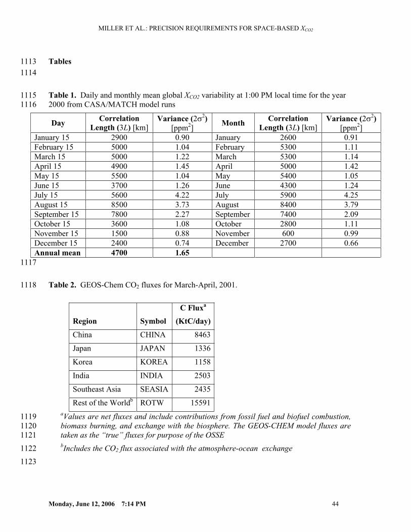
MILLER ET AL.: PRECISION REQUIREMENTS FOR SPACE-BASED XCO2
Tables11131114
11151116
Table 1. Daily and monthly mean global XCO2 variability at 1:00 PM local time for the year 2000 from CASA/MATCH model runs
DayCorrelation
Length (3L) [km]Variance (2 2)
[ppm2] MonthCorrelation
Length (3L) [km]Variance (2 2)
[ppm2]January 15 2900 0.90 January 2600 0.91February 15 5000 1.04 February 5300 1.11March 15 5000 1.22 March 5300 1.14April 15 4900 1.45 April 5000 1.42May 15 5500 1.04 May 5400 1.05June 15 3700 1.26 June 4300 1.24July 15 5600 4.22 July 5900 4.25August 15 8500 3.73 August 8400 3.79September 15 7800 2.27 September 7400 2.09October 15 3600 1.08 October 2800 1.11November 15 1500 0.88 November 600 0.99December 15 2400 0.74 December 2700 0.66Annual mean 4700 1.65
1117
1118 Table 2. GEOS-Chem CO2 fluxes for March-April, 2001.
Region Symbol
C Fluxa
(KtC/day)
China CHINA 8463
Japan JAPAN 1336
Korea KOREA 1158
India INDIA 2503
Southeast Asia SEASIA 2435
Rest of the Worldb ROTW 15591aValues are net fluxes and include contributions from fossil fuel and biofuel combustion, biomass burning, and exchange with the biosphere. The GEOS-CHEM model fluxes are taken as the “true” fluxes for purpose of the OSSE
111911201121
1122
1123
bIncludes the CO2 flux associated with the atmosphere-ocean exchange
Monday, June 12, 2006 7:14 PM 44
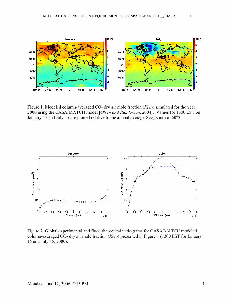
MILLER ET AL.: PRECISION REQUIREMENTS FOR SPACE-BASED XCO2 DATA 1
Figure 1. Modeled column-averaged CO2 dry air mole fraction (XCO2) simulated for the year2000 using the CASA/MATCH model [Olsen and Randerson, 2004]. Values for 1300 LST on January 15 and July 15 are plotted relative to the annual average XCO2 south of 60oS.
Figure 2. Global experimental and fitted theoretical variograms for CASA/MATCH modeled column-averaged CO2 dry air mole fraction (XCO2) presented in Figure 1 (1300 LST for January 15 and July 15, 2000).
Monday, June 12, 2006 7:13 PM 1

MILLER ET AL.: PRECISION REQUIREMENTS FOR SPACE-BASED XCO2 DATA 2
Figure 3. Locally-estimated correlation lengths for CASA/MATCH modeled column-averagedCO2 dry air mole fraction (XCO2) presented in Figure 1 (1300 LST for January 15 and July 15, 2000).
Figure 4. Locally-estimated variance for CASA/MATCH modeled column-averaged CO2 dry air mole fraction (XCO2) presented in Figure 1 (1300 LST for January 15 and July 15, 2000).
Monday, June 12, 2006 7:13 PM 2
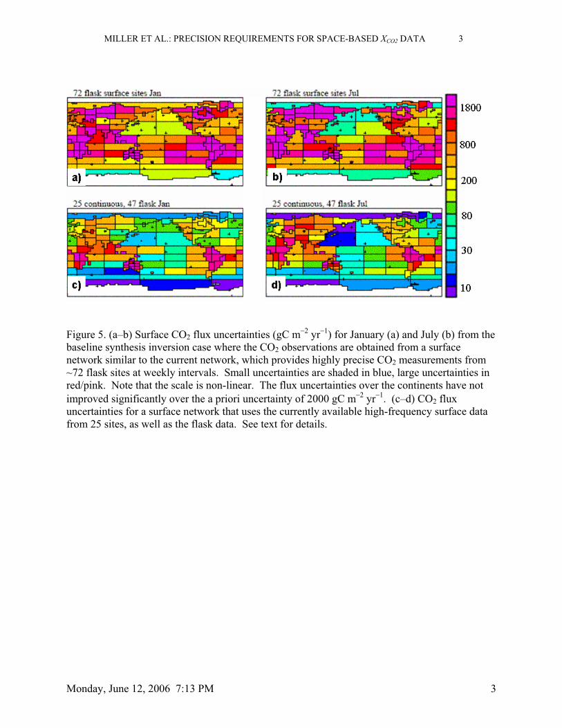
MILLER ET AL.: PRECISION REQUIREMENTS FOR SPACE-BASED XCO2 DATA 3
Figure 5. (a–b) Surface CO2 flux uncertainties (gC m 2 yr 1) for January (a) and July (b) from the baseline synthesis inversion case where the CO2 observations are obtained from a surface network similar to the current network, which provides highly precise CO2 measurements from~72 flask sites at weekly intervals. Small uncertainties are shaded in blue, large uncertainties in red/pink. Note that the scale is non-linear. The flux uncertainties over the continents have not improved significantly over the a priori uncertainty of 2000 gC m 2 yr 1. (c–d) CO2 fluxuncertainties for a surface network that uses the currently available high-frequency surface data from 25 sites, as well as the flask data. See text for details.
Monday, June 12, 2006 7:13 PM 3
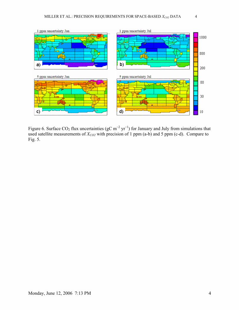
MILLER ET AL.: PRECISION REQUIREMENTS FOR SPACE-BASED XCO2 DATA 4
Figure 6. Surface CO2 flux uncertainties (gC m 2 yr 1) for January and July from simulations that used satellite measurements of XCO2 with precision of 1 ppm (a-b) and 5 ppm (c-d). Compare to Fig. 5.
Monday, June 12, 2006 7:13 PM 4

MILLER ET AL.: PRECISION REQUIREMENTS FOR SPACE-BASED XCO2 DATA 5
Figure 7. Surface CO2 concentration differences (ppm) associated with a +0.1 ppm bias in the XCO2 observations acquired over land. The locations of the surface CO2 monitoring network stations are shown as black circles.
Monday, June 12, 2006 7:13 PM 5

MILLER ET AL.: PRECISION REQUIREMENTS FOR SPACE-BASED XCO2 DATA 6
Figure 8. Surface CO2 flux errors (gC m 2 yr 1) inferred from an inversion of XCO2 data biased +0.1 ppm over land that have been corrected using the XCO2 bias map given in Fig.7. Most regions show differences smaller than 10 gC m 2 yr 1 and the differences are no longer spatiallycoherent.
Monday, June 12, 2006 7:13 PM 6

MILLER ET AL.: PRECISION REQUIREMENTS FOR SPACE-BASED XCO2 DATA 7
Figure 9. Asian geographical regions used in the inversion analysis. CO2 surface fluxes from each region are given in Table 2.
Monday, June 12, 2006 7:13 PM 7

MILLER ET AL.: PRECISION REQUIREMENTS FOR SPACE-BASED XCO2 DATA 8
Figure 10. (a) Modeled XCO2 values for March 2001. (b) Comparison of a posteriori flux estimates (calculated with an observation error of 0.3%) with true and a priori fluxes. Red bars:a posteriori fluxes, Blue bars: a priori fluxes, Black bars: true fluxes. Error bars show an uncertainty of 1 .
Monday, June 12, 2006 7:13 PM 8
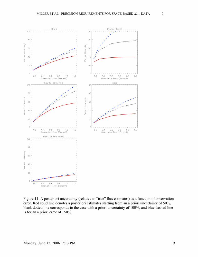
MILLER ET AL.: PRECISION REQUIREMENTS FOR SPACE-BASED XCO2 DATA 9
Figure 11. A posteriori uncertainty (relative to “true” flux estimates) as a function of observation error. Red solid line denotes a posteriori estimates starting from an a priori uncertainty of 50%, black dotted line corresponds to the case with a priori uncertainty of 100%, and blue dashed line is for an a priori error of 150%.
Monday, June 12, 2006 7:13 PM 9

MILLER ET AL.: PRECISION REQUIREMENTS FOR SPACE-BASED XCO2 DATA 10
Figure 12. Flux errors (gC m 2 yr 1) for January and July are shown for orbits with sampling times of 1100 and 1400 LST for cases with SZA < 75 (a, b) and with a sampling time of 1400 LST for SZA < 60 (c). Small uncertainties are shaded in blue, large uncertainties in red/pink. Note that the scale is non-linear. Compare to Fig. 6a-b.
Monday, June 12, 2006 7:13 PM 10

MILLER ET AL.: PRECISION REQUIREMENTS FOR SPACE-BASED XCO2 DATA 11
Figure 13 MODIS Aqua clear-sky fraction map for 24 August, 2002.
Monday, June 12, 2006 7:13 PM 11

MILLER ET AL.: PRECISION REQUIREMENTS FOR SPACE-BASED XCO2 DATA 12
Aqua MODIS Clear Sky Fraction: 5 Nov 2000
Pixel Area/km2
2 4 16 36 64 100 144 256 400
Cle
ar S
ky F
ract
ion/
per
cent
10
15
20
25
30
Figure 14 Global clear-sky frequency vs. spatial resolution computed using the MODIS 1 km cloud product
Monday, June 12, 2006 7:13 PM 12
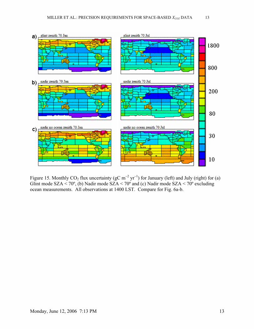
MILLER ET AL.: PRECISION REQUIREMENTS FOR SPACE-BASED XCO2 DATA 13
Figure 15. Monthly CO2 flux uncertainty (gC m 2 yr 1) for January (left) and July (right) for (a)Glint mode SZA < 70º, (b) Nadir mode SZA < 70º and (c) Nadir mode SZA < 70º excluding ocean measurements. All observations at 1400 LST. Compare for Fig. 6a-b.
Monday, June 12, 2006 7:13 PM 13

MILLER ET AL.: PRECISION REQUIREMENTS FOR SPACE-BASED XCO2 DATA 14
Figure 16. Spatial variations of simulated column mean CO2 mixing ratios (ppm) for 4 different times during July 28, 1997 on the 1-km grid centered at the WLEF tower.
Monday, June 12, 2006 7:13 PM 14