Precision radial velocities of 15 M5–M9 dwarfs

MNRAS 439, 3094–3113 (2014) doi:10.1093/mnras/stu172Advance Access publication 2014 February 20

Precision radial velocities of 15 M5–M9 dwarfs

J. R. Barnes,1‹ J. S. Jenkins,2 H. R. A. Jones,1 S. V. Jeffers,3 P. Rojo,2 P. Arriagada,4

A. Jordan,4 D. Minniti,4,5 M. Tuomi,1,6 D. Pinfield1 and G. Anglada-Escude7

1Centre for Astrophysics Research, University of Hertfordshire, College Lane, Hatfield, Hertfordshire AL10 9AB, UK2Departamento de Astronomıa, Universidad de Chile, Camino del Observatorio 1515, Las Condes, Santiago, Chile3Institut fur Astrophysik, Georg-August-Universitat, Friedrich-Hund-Platz 1, Friedrich-Hund-Platz 1, D-37077 Gottingen, Germany4Instituto de Astrofısica, Pontificia Universidad Catolica de Chile, Av. Vicuna Mackenna 4860, 7820436 Macul, Santiago, Chile5Vatican Observatory, I-V00120 Vatican City State, Italy6University of Turku, Tuorla Observatory, Department of Physics and Astronomy, Vaisalantie 20, FI-21500 Piikkio, Finland7Astronomy Unit, School of Physics and Astronomy, Queen Mary, University of London, Mile End Road, London E1 4NS, UK

Accepted 2014 January 21. Received 2014 January 21; in original form 2013 October 26

ABSTRACTWe present radial velocity measurements of a sample of M5V–M9V stars from our Red-OpticalPlanet Survey, operating at 0.652–1.025 µm. Radial velocities for 15 stars, with rms precisiondown to 2.5 m s−1 over a week-long time-scale, are achieved using thorium–argon referencespectra. We are sensitive to planets with mp sin i ≥ 1.5 M⊕ (3 M⊕ at 2σ ) in the classicalhabitable zone, and our observations currently rule out planets with mp sin i > 0.5 MJ at 0.03 aufor all our targets. A total of 9 of the 15 targets exhibit rms < 16 m s−1, which enables us to ruleout the presence of planets with mp sin i > 10 M⊕ in 0.03 au orbits. Since the mean rotationvelocity is of the order of 8 km s−1 for an M6V star and 15 km s−1 for M9V, we avoid observingonly slow rotators that would introduce a bias towards low axial inclination (i � 90◦) systems,which are unfavourable for planet detection. Our targets with the highest v sin i values exhibitradial velocities significantly above the photon-noise-limited precision, even after accountingfor v sin i. We have therefore monitored stellar activity via chromospheric emission fromthe Hα and Ca II infrared triplet lines. A clear trend of log10(LHα/Lbol) with radial velocityrms is seen, implying that significant starspot activity is responsible for the observed radialvelocity precision floor. The implication that most late M dwarfs are significantly spotted,and hence exhibit time varying line distortions, indicates that observations to detect orbitingplanets need strategies to reliably mitigate against the effects of activity-induced radial velocityvariations.

Key words: techniques: radial velocities – planets and satellites: detection – stars: activity –stars: atmospheres – stars: low-mass – planetary systems.

1 IN T RO D U C T I O N

Although the solar neighbourhood is dominated by low-mass stars,the late M dwarf population has remained largely beyond the reachof optical precision radial velocity (RV) surveys. In order to addressthis major parameter space, dedicated instruments have been pro-posed that would instead operate at longer wavelengths, at the peakof the energy distribution of low-mass stars (Jones et al. 2008).Upcoming instruments are now being constructed, and includethe Habitable Zone Planet Finder (Mahadevan et al. 2012) andCARMENES, the Calar Alto high-Resolution search for M dwarfswith Exo-earths with Near-infrared and optical Echelle Spectrom-eters (Quirrenbach et al. 2012). However, while a number of well-

� E-mail: [email protected]

established instruments with proven stability at earlier spectral typeshave also reported precision RVs for early M dwarfs, the CRyo-genic high resolution InfraRed Echelle Spectrometer (CRIRES)survey (Bean et al. 2010) and the Red-Optical Planet Surve (ROPS;Barnes et al. 2012, hereafter B12) have reported precision RVs atthe ∼10 m s−1 level for late M dwarfs (M6V–M9V) with existinginstrumentation. Reiners (2009) has also reported ∼10 m s−1 sta-bility on the flaring M6 dwarf CN Leo. Working in the infraredK band, Bean et al. (2010) reported 11.7 m s−1 for Proxima Cen,and 5.4 m s−1 after observations were binned together. On the otherhand, B12, working in the red-optical (0.62–0.90 µm), found thatwhile propagated errors were at the ∼10 m s−1 level, the rms scat-ter was 16–35 m s−1 in the most stable targets. Until CRIRES isupgraded to a cross-dispersed, multi-order instrument, Ultravioletand Visual Echelle Spectrograph (UVES) has substantially morewavelength coverage with reasonable signal-to-noise (S/N) from

C© 2014 The AuthorsPublished by Oxford University Press on behalf of the Royal Astronomical Society

at Universidad de C

hile on September 29, 2014

http://mnras.oxfordjournals.org/

Dow

nloaded from

mailto:[email protected]


M dwarf radial velocities with ROPS 3095

which RVs may be derived. UVES has also already demonstrated 2–2.5 m s−1 precision over 7 yr working with an I2 cell (Zechmeister,Kurster & Endl 2009) in the 5000–6000 Å range. However, by∼6500 Å, I2 lines become weak (<10 per cent of the normalizedcontinuum) and are barely visible beyond 7000 Å. Hence, I2 gascells cannot be used in the red part of the optical, beyond thesewavelengths.

The first planet orbiting an M dwarf was reported by Delfosseet al. (1998) and Marcy et al. (1998) nearly a decade after thefirst low-mass companion to the main-sequence star HD 114762(Latham et al. 1989), which may be either a brown dwarf or mas-sive planet, depending on the unknown orbital inclination. GJ 876b, orbiting its parent M4V star in a 61 d orbit is a giant planet,which is perhaps not surprising given that close-orbiting compan-ions are the easiest to detect with few epochs of observations usingRV techniques. However, while close-orbiting planets have beenpredicted to be relatively common for early M dwarf samples (seeSection 1.1 below), only ∼50 per cent of the M dwarf planets withmass estimates (16 from a total of 31)1 possess masses �0.3 MJ.The remaining 15 planets have minimum masses implying Super-Earth to Neptune-mass companions. GJ 876 b is only one of fourplanets so far detected orbiting GJ 876, and in fact two of the plan-ets possess masses of only 5.8 and 12.5 M⊕. In addition, amongstthe Kepler candidates first reported by Borucki et al. (2011) andconfirmed by a number of authors (Fabrycky et al. 2012; Muirheadet al. 2012; Steffen et al. 2013), 14 planets have been identified withradii ≤3 R⊕, whilst no transiting hot Jupiters have been detected. Todate these findings confirm earlier predictions that Neptune-massand Earth-mass planets are expected in greater numbers in orbitaround M stars (Ida & Lin 2005).

1.1 Rocky planet occurrence rates and the M dwarfhabitable zone

Bonfils et al. (2013) have calculated phase-averaged detection lim-its for individual stars, which enable the survey efficiency of theHARPS (High Accuracy Radial velocity Planet Searcher) early Mdwarf sample to be determined. These detection limits enable cor-rections to be made for incompleteness, allowing occurrence ratesto be estimated. The frequency of HZ planets, η⊕ (where 1 <

m sin i < 10 M⊕), orbiting early M dwarfs is found to be 0.36+0.25−0.10.

From the Kepler sample, Dressing & Charbonneau (2013) estimatedη⊕ = 0.90 +0.04

−0.03 for M dwarf planets up to 4 R⊕. With revised esti-mates of habitable zones (HZ; Kopparapu et al. 2013), Kopparapu(2013) used the 95 Kepler planet candidates orbiting 64 low-masshost stars to similarly place conservative estimates of η⊕ = 0.51+0.10

−0.20

for M dwarf planets with radii in the range 0.5–2 R⊕. Bonfils et al.(2013) find that the majority of early M dwarf planets are clusteredin few-day to tens of days orbits, continuing the trend with semi-major axis distribution observed by Currie (2009). By extrapolation,we might expect late M dwarf planets in orbits up to a few tens ofdays.

The centre of the continuous HZ for an M6V star is estimatedto be ∼0.045 au (Kopparapu et al. 2013). Hence, a 7.5 M⊕ planetwould induce a K∗ = 10 m s−1 signal with an 11.0 d period. Al-though Kopparapu et al. (2013) do not make HZ estimates for lowmasses, based on a simple flux and mass scaling, we estimate thatan M9V star HZ would be centred at ∼0.023 au, with a 7.5 M⊕

1 http://exoplanets.org

planet inducing a 15.8 m s−1 signal with a 4.4 d period. Observa-tions spanning a 6 d period (which we present in this paper) thusoffer the potential to sample 55 per cent of an M6V HZ period,and greater than a complete orbit for an M9V star. By defining acontinuous HZ, the range of possible orbital periods for habitableplanets are extended. For instance, Kopparapu et al. (2013) defineinner moist greenhouse and outer greenhouse limits, which extendthe range of periods for an M6V habitable planet from ∼6 d to amaximum of ∼17 d.

1.2 ROPS sample

Our choice of targets was based on a number of factors includingvisibility and brightness. In order to obtain sufficient S/N in thespectra in exposures limited to no more than 1800 s, we limitedthe selection to M5–M9 dwarfs with apparent I-band magnitudes�14.5. A number of stars in common with our initial observationsmade with the Magellan Inamori Kyocera Echelle (MIKE) spectro-graph at Magellan Clay (B12) have been retained. Additional targetswere selected, ensuring that a range of spectral types were includedwith low-moderate v sin i values. Because M stars, and particularlylate M stars on the whole, are not effectively spun down, those starslater than M6V tend to be moderate rotators on the whole. Jenk-ins et al. (2009) found that M6V stars on average possess v sin i∼8 km s−1, whereas this rises to ∼15 km s−1 for M9V. This obvi-ously has important consequences for RV precision, especially ifmagnetic activity phenomena affect the rotation profiles. Becausemoderate rotation is found on average, selecting only the slowestrotating stars with v sin i ≤ 5 km s−1 is likely to bias a target sampleto low axial inclination (i � 90◦) systems (i.e. with rotation axisaligned along the line of sight to the observer), for which detectionof planets is less favourable. In order to characterize the effects ofactivity for this and future surveys, we included moderate rotatorsin our sample. The objects were selected for which v sin i was onthe whole well measured (Mohanty & Basri 2003; Reiners & Basri2010). In addition, following the procedures detailed in Jenkins et al.(2009), we have also obtained the first v sin i measurements for twoof the targets in our sample, GJ 3076 and GJ 3146, as indicated inTable 1.

In this paper, we investigate the methods by which precisionRVs can be achieved with existing instrumentation, extending thesearch of optical spectrometers into the 0.65–1.025 µm wavelengthregion, where no established simultaneous reference fiducial hasbeen tested. In Section 3, we outline our master wavelength cali-bration procedure. The use of tellurics for wavelength calibrationis investigated in Section 4 using an analysis similar to that car-ried out by Figueira et al. (2010) for HARPS observations of G-type stars. We derive RVs for Proxima Centauri using only telluriclines to enable us to determine the simultaneous wavelength solu-tion. In Section 5, we present the RV measurement procedures forour ROPS sample, discussing our wavelength calibration procedure(Section 5.2), applicable particularly to UVES observations, beforepresenting RVs for our 15 M5V–M9V targets from four epochs ofobservations spread over a week-long time-scale (Section 5.3). Fi-nally, we discuss our findings (Section 5.4) and prospects for futureobservations (Section 6).

2 O BSERVATI ONS

In this paper, we utilize observations made during our own observingcampaign in 2012 July. We also use data taken from the EuropeanSouthern Observatory (ESO) archive.

MNRAS 439, 3094–3113 (2014)

at Universidad de C



Dow

nloaded from

http://exoplanets.org


3096 J. R. Barnes et al.

Table 1. List of targets observed with UVES with estimated spectral types, I-band magnitudes, exposure times and v sin i values (columns 1 to 5). Themeasured v sin i values are taken from Mohanty & Basri (2003), Jenkins et al. (2009) and Reiners & Basri (2010). We derived v sin i’s for GJ 3076 and GJ3146 (denoted by *) using the procedures we adopted in Jenkins et al. (2009). We also list details for Proxima Centauri and the mean rms of 5.2 m s−1, afteratmospheric correction for all three nights, is given. The exposure times† for Proxima Centauri were variable, ranging between 11 and 500 s; however, 74 percent of the observations were made with 100 s exposures. Extracted S/N ratio and S/N ratio after deconvolution are tabulated in columns 6 and 7. Column 8lists the total number of observations, Nobs on each target and column 9 gives the rms scatter using an Nobs − 1 correction to account for the small number ofobservations for each object (see Section 5.3). In columns 10, 11 and 12, we list rms values after applying bisector corrections derived from the stellar line (L),telluric line (T), and both lines (L-T). Discussion of the results is given in Section 5.3.

Star SpT Imag Exp v sin i S/N Mean S/N Nobs rms rms rms rms(s) (km s−1) (m s−1) (m s−1) (m s−1) (m s−1)

Extracted Decon No corr L corr T corr L-T corr

GJ 3076 M5V 10.9 400 17.1* 77 ± 10 6120 4 100.7 92.3 67.6 44.5GJ 1002 M5.5V 10.2 300 ≤3 106 ± 12 9110 4 29.4 5.1 12.9 23.6GJ 1061 M5.5V 9.5 300 ≤5 142 ± 12 12 150 5 4.23 2.4 2.4 2.8LP 759-25 M5.5V 13.7 1500 13 38 ± 5 2810 4 106.8 79.9 70.6 65.9GJ 3146 M5.5V 11.3 600 12.4* 60 ± 10 4920 4 87.2 47.1 80.2 7.75GJ 3128 M6V 11.1 350 ≤5 65 ± 3 5590 4 24.4 11.5 24.1 15.6Proxima Centauri M6V 6.9 100† 2 191 ± 22 12 900 561 5.2 – – –GJ 4281 M6.5V 12.7 1200 7 49 ± 6 4240 4 36.7 11.7 12.0 15.3SO J025300.5+165258 M7V 10.7 350 ≤5 95 ± 12 8280 4 15.2 12.4 12.5 14.6LP 888-18 M7.5V 13.7 1500 ≤3 36 ± 3 2790 4 45.3 35.3 31.6 38.0LHS 132 M8V 13.8 500 ≤5 37 ± 2 3160 4 12.3 12.3 7.7 9.092MASS J23062928−0502285 M8V 14.0 1500 6 38 ± 1 2890 4 29.0 14.2 16.9 10.0LHS 1367 M8V 13.9 1500 ≤5 32 ± 3 2470 4 22.7 15.3 16.1 22.5LP 412-31 M8V 14 1200 12 26 ± 7 1850 3 253.2 222.6 248.9 119.62MASS J23312174−2749500 M8.5V 14.0 1500 6 37 ± 2 2890 4 37.2 36.7 29.5 22.32MASS J03341218−4953322 M9V 14.1 1500 8 33 ± 2 2810 4 11.2 6.37 6.92 8.37

2.1 ROPS observations with UVES

We observed 15 m dwarf targets with the UVES at the 8.2 m VeryLarge Telescope (VLT, UT2). Observations were made with a0.8 arcsec slit, which give a resolution of R ∼ 54 000. We ob-served on four half nights spread over a period of six nights in total,on 2012 July 23, 24, 26 and 29 (UTC). Short orbital periods mightbe expected by extrapolating the tens of days orbits, found amongstearly M dwarfs (Bonfils et al. 2013), to the late M dwarf population.Additionally, the observing strategy enabled the stability of UVESand our measurement precision to be characterized on week-longtime-scales. Although UVES offers the ability to simultaneouslyrecord observations at shorter and longer wavelengths, we opted tomake observations in the red arm only since mid-to-late M starsoutput little flux short of 6000 Å. In B12, we found the ratio of fluxin the 7000–9000 Å region compared with the 5000–7000 Å regionto be 11.5 and 19 for M5.5V and M9V spectra, respectively. Thisestimate included the throughput of the 6.5 m Magellan Clay andMIKE spectrograph.

Working in the red-optical (i.e. 0.6–1.0 µm) poses a particularchallenge in that there are no currently operating echelle spectrom-eters coupled with 8 m class telescopes that offer simultaneous cali-bration. Regular wavelength observations for calibration are crucialif precisions of the order of m s−1 are to be achieved from high-resolution RV information. Although UVES possesses an iodinecell, the absorption lines of I2 do not extend far above 6500 Å,and are already very weak, with line depths of only a few per centof the normalized continuum. We have therefore opted to utilizenear-simultaneous observations of thorium–argon (ThAr) arc lamplines, coupled with the relative stability of UVES in order to achievesub-m s−1 precision on our target population of late M stars. SinceThAr lamps exhibit many lines for calibration, and are generallyalways available by default with echelle spectrometers working atoptical wavelengths, we made regular observations with the com-

parison lamp available with UVES. A calibration was included inthe observing block associated with each observed target and wastaken immediately after each science frame. Further details on thecalibration procedures are given in Section 3 and following sections.The observing conditions over the four half nights were very good,with seeing estimates in the range 0.7–1.2 for targets observed atairmasses <1.5. Our targets are listed in Table 1.

2.2 Proxima Centauri observations

Proxima Centauri has been shown by Endl & Kurster (2008) to bestable to 3.11 m s−1 over a 7 yr period and thus we consider thisto be a good target to pursue as a calibrator for our techniques.Data taken with UVES, spanning five nights, with observationsmade on three nights and single night gaps, were obtained fromthe ESO data archive. These data were initially taken as part ofa multiwavelength survey of Proxima Centauri (GJ 551) and arepresented in Fuhrmeister et al. (2011). Approximately 560 spectraof Proxima Centauri were continuously recorded on each of thethree nights on 2009 March 10, 12 and 14, spanning 8 h per nightwith altitudes corresponding to an airmass range of 2.41–1.27. A slitwidth of 1 arcsec gives a spectral resolution, R � 43 000, in the redarm of UVES, while the extreme airmass range of the observationsled to seeing that varied from 1.4 arcsec at high airmass, down to∼0.6 arcsec at low airmass. The CCD readout was binned in thewavelength direction by a factor of 2, resulting in an average pixelincrement of 2.4 km s−1. The rotation velocity of Proxima Centauri,at v sin i = 2 km s−1, means that spectral resolution (equivalent to∼6 km s−1) dominates the line width.

2.3 Data extraction

The data sets for both our ROPS sample (Section 2.1) and ProximaCentauri (Section 2.2) were flat-field corrected by using combined

MNRAS 439, 3094–3113 (2014)

at Universidad de C



Dow

nloaded from



exposures taken with an internal tungsten reference lamp. Since fewcounts are recorded in the reddest orders of the Massachusetts In-stitute of Technology Lincoln Laboratory (MITLL) CCD (owing tothe spectrograph efficiency and low quantum efficiency of the CCDlongwards of 1.0 µm), where of the order of 10 000 counts couldbe achieved with 14 s exposures compared with a peak of 40 000counts, an additional 30 flat-field frames were taken in addition tothe standard calibrations for the ROPS (Section 2.1) data set. Theworst cosmic ray events were removed at the pre-extraction stageusing the Starlink FIGARO (Shortridge 1993) routine bclean (theStarlink software is currently distributed by the Joint AstronomyCentre2). The spectra were extracted using ECHOMOP’s implementa-tion of the optimal extraction algorithm developed by Horne (1986).ECHOMOP rejects all but the strongest sky lines (Barnes et al. 2007)and propagates error information based on photon statistics andreadout noise throughout the extraction process.

3 WAV E L E N G T H C A L I B R AT I O N

Wavelength calibration at the m s−1 level is required if precisionRVs are to be achieved. To this end, a great deal of effort has beenexpended in order to obtain accurate wavelengths for spectral cal-ibration references (e.g. Gerstenkorn & Luc 1978). Despite recentwork that has identified new sources for calibration, suitable refer-ence lines are often limited in the wavelength regions that they span.Mahadevan & Ge (2009) have identified a number of molecular gascells that could be used to span the H band, while LASER combtechnology has also been used to demonstrate ∼10 m s−1 precisionon sky in the H band (Ycas et al. 2012). Although new calibrationsources, rich in lines, have also been identified in the red part of theoptical (Redman et al. 2011), ThAr still remains the most regularlyused and only available calibration source for optical and infraredhigh-resolution spectrometers, although with relatively few lines inthe near-infrared (>1 µm).

3.1 Master wavelength calibration

ThAr wavelengths published by Lovis & Pepe (2007) were usedto identify stable lines for wavelength calibration. This line list isestimated to enable a calibration (i.e. global) rms to better than20 cm s−1 for HARPS. Pixel positions were initially identified fora single arc using a simple Gaussian fit. For each subsequent arc,a cross-match was made, followed by a multiple-Gaussian (up tothree profiles) fit around each identified line using a Levenberg–Marquardt fitting algorithm (Press et al. 1986) to obtain the pixelposition of each line centre. The Lovis & Pepe line list was opti-mized for HARPS at R = 110 000, while our observations weremade at R ∼ 50 000 necessitating rejection of some lines thatshowed blending. Using a multiple-Gaussian fit enables the effectof any nearby lines to be accounted for in the fit that also includeda first-order (straight line) background. Any lines closer than theinstrumental full width at half-maximum (FWHM) were not used.Finally for each order, any remaining outliers were removed afterfitting a cubic polynomial. In addition, any lines that were not con-sistently yielding a good fit for all arc frames throughout both nights(to within 3σ of the cubic fits) were removed.

The ThAr observation following each star on the second night waschosen arbitrarily as the reference solution for that star. The wave-lengths were then incrementally updated for all other observationsof each star using the methods that we describe in Sections 4.2 and

2 http://starlink.jach.hawaii.edu/starlink

5.2, which are aimed at minimizing systematics in the wavelengthsolutions from one observation to the next. A total wavelength spanof 6519–10 252 Å is covered by the EEV and MITLL chips at thenon-standard 840 nm setting of UVES. An order that falls betweenthe two CCDs cannot be used and must be accounted for correctlyin the two-dimensional solution. The candidate ThAr lines weresubjected to a two-dimensional fit of wavelength versus extractedorder (cross-dispersion) for each CCD independently. For each star,an arbitrary reference solution with a two-dimensional polynomialfit using four coefficients in the wavelength direction and six coef-ficients in the cross-dispersion (order) direction was made:

λ(x, y) =3∑

i=0

aixi

5∑j=0

bjyj , (1)

where a and b are the polynomial coefficients that we fit for. x and yare the pixel number and order number, respectively, and i and j arethe powers in x and y for each coefficient. By iteratively rejectingoutlying pixels from the fit, we found that of the input 573 lines,clipping the furthest outliers yielded the most consistent fit fromone solution to the next. Typically, 15–20 lines were rejected beforea final fit was produced for each observation. The zero-point rms(i.e. the rms by combining all lines) for the master wavelength cal-ibrations is found to be ∼5–5.5 and ∼6–6.5 m s−1 for the EEV andMITLL chips, respectively, and represents the goodness of fit of thepolynomial. These values are dominated by a systematic differencebetween the wavelengths and the two-dimensional fit. The variabil-ity in the wavelength solution for a given set of RV measurements(i.e. for each star) is thus important and ultimately determines theprecision that can be achieved. We discuss this further in Section 5.2,but note here that this variability is an order of magnitude smaller(i.e. <1 m s−1) than the zero-point rms values quoted above.

The appropriate wavelength solution for each observation canbe obtained through a simultaneous measurement, by using the tel-luric lines, or a near-simultaneous measurement by using the nearbyThAr reference frame. In each instance, the corrections are deter-mined as pixel shifts and applied to the master wavelength solution.This procedure enables wavelength corrections to be applied, al-lowing for low-order shifts and stretches (due to mechanical effectsand temperature/pressure changes). In other words, allowing moredegrees of freedom for each solution can lead to poor fits in the firstand last orders, near the order edges, and in regions where theremay be fewer lines. Low-order corrections correctly describe thechanges in the instrument while minimizing variability in the fits.We describe the two methods adopted in this paper for updatingthe wavelength, using telluric lines (Section 4.2) and ThAr lines(Section 5.2).

4 T E L L U R I C S A S A WAV E L E N G T HR E F E R E N C E

The benefit of utilizing telluric lines to obtain a local wavelengthsolution is that the wavelengths are derived from the very observa-tion of the star itself and are therefore simultaneous. The telluricspectrum essentially follows the same light path as the star throughthe Earth’s atmosphere, the telescope and the spectrograph, andis thus subject to the same systematics. The calibration procedurecould be seen as analogous to that first adopted by Marcy & Butler(1992) and Butler et al. (1996) if the atmosphere of the Earth couldbe well characterized and calibrated for. In addition, at the timeof observations, there were no optical 8 m class spectrometers thatenable simultaneous ThAr observations to be made.

MNRAS 439, 3094–3113 (2014)

at Universidad de C



Dow

nloaded from

http://starlink.jach.hawaii.edu/starlink



The stability of telluric lines as reference fiducials has been inves-tigated by a number of authors. Griffin & Griffin (1973), for exam-ple, made some initial attempts to identify lines in the 6841–7424 Åregion, estimating uncertainties at the 1–2 mÅ level, equivalent to∼40–90 m s−1. The most complete list of ab initio line strengthsand positions for water has now been calculated by Barber et al.(2006) and is now routinely used in model atmosphere data basesthat supply molecular information for many molecules (Rothmanet al. 2009). Bands of telluric molecular absorption lines pose achallenge for any ground-based observations and are seen fromthe mid-optical, becoming stronger and wider into the infrared. Inthe red-optical, at wavelengths greater than 6500 Å, significant O2

absorption bands with bandheads at ∼6865 and ∼7595 Å appear,the latter showing strong absorption with saturation in some lines.H2O bandheads at 6450, 7170 and 8100 Å exhibit increasing widthsfrom ∼100 Å to several 100 Å; however, the band covering 8890–9950 Å is by far the most extensive at wavelengths short of 1 µm.Gray & Brown (2006) were able to achieve empirical precisions of∼25 m s−1 using strong H2O absorption lines in the 6222–6254 Åregion formed in the optical path of the coude echelle spectrographused. This procedure had the advantage of minimizing atmosphericprojection effects such as change in airmass.

Figueira et al. (2010) instead took advantage of night-long ob-servations made on bright stable stars with the HARPS, locatedat the ESO 3.6 m at La Silla. They found clear nightly trends ofthe RV variations of the O2 absorption band as measured in thespectra of τ Ceti (HD 10700), μ Ara (HD 160691) and ε Eri (HD20794). Empirical fits were made to the velocities using a simplemodel that included a linear airmass term (fixed, with magnitude of∼ 20 m s−1), a projection of the wind velocity along the line of sightof the telescope (encompassing both magnitude and direction) and afixed calibration offset term. Such a procedure enabled typical mea-surement precisions over week-long time-scales of 4.5–10 m s−1 tobe made for observations at less than 1.5 airmass (>41.◦8) and2.4–4 m s−1 when restricting observations to less than 1.1 airmass(>65.◦4). Over a period of 6 years, the precision was found to be ofthe order of 10 m s−1.

4.1 Precision RVs of Proxima Centauri

The opportunity to study the stability of telluric lines alone forupdating the wavelength solution and providing a stable cross-correlation reference against which to make precision RV measure-ments is afforded by the archival observations of Proxima Centauri,already outlined in Section 2.2 and initially published in Fuhrmeisteret al. (2011). We intended to characterize the stability and behaviourof UVES for our RV measurement technique by making use of the∼560 archival observations taken over three nights, with an inten-tion of extending the method to our ROPS sample. In addition, thiskind of study is not possible with our 2012 July observations sincewe only observed each target once per night, which precludes mon-itoring stability on minute- to hour-long time-scales. Kurster et al.(1999) showed that Proxima Centauri is stable to the 54 m s−1 level,while more recent results from Endl & Kurster (2008) have shownit to be stable to 3.11 m s−1 over a 7 yr period, but quote an av-erage propagated uncertainty of 2.34 m s−1 in their measurements,indicating an additional unaccounted for source of noise.

The seeing variations of 1.4 arcsec at high airmass, down to∼0.6 arcsec at low airmass, when viewed with a 1 arcsec slit of-fer a less than ideal match since the star does not completely fillthe slit. This results in changes in illumination of the echelle, lead-ing to RVs that can potentially vary at the m s−1 to several tens of

m s−1 level. Since the CCD readout was binned by a factor of 2 inthe wavelength direction, the mean pixel increment of 2.4 km s−1

is twice that of the full 1.2 km s−1 mean readout increment usedfor the ROPS targets. Only one ThAr frame per night was recordedduring the automated calibration procedures executed by UVESeach night. As a result, it is impossible to track any drift of thespectrograph through the night, or in this instance, to investigateour ability to use the ThAr frames as a near-simultaneous referencefiducial. During extraction, we also discovered that on 2009 March10 and 14, a regular half hour, cyclic shift of the order of 1 km s−1

appears in the RVs. The origin of this cyclical behaviour is unclear,but it appears to coincide with times at which the seeing was verygood. We believe that it is related to the mismatch of seeing andslit width where the autoguider may have been fooled into makingonly occasional corrections that have resulted in significant echelleillumination change.

4.2 RV measurement procedure

Starting with the two-dimensional wavelength solution describedin Section 3.1, a method of updating the local wavelength solu-tion for each observation must be obtained. No special wavelengthcalibrations were made during the observing sequence of ProximaCentauri, and only one ThAr spectrum was recorded during thestandard calibrations for each night. We therefore investigated theuse of the abundant H2O and O2 in the red-optical to update thewavelength solutions.

The weather conditions on the first night were particularly dry,with relative humidity variations in the 2–14 per cent range (asrecorded for the telescope dome in the observation headers). On thesecond and third nights, the relative humidity varied in the ranges48–54 and 22–28 per cent. The increased water column is clearlyevident in the H2O lines as illustrated in Fig. 1. This additionallyserves to illustrate why the use of water lines for precision RV workcan prove challenging. With careful selection, it is in fact possibleto select H2O lines that are not blended with other lines and thatalso do not vary so greatly in strength as to become insignificantrelative to the continuum level noise. Since Fig. 1 illustrates theextremes of the telluric line variations during the Proxima Centauri

Figure 1. Spectral region 9510–9570 Å illustrating the change in humiditybetween 2009 March 10 (low humidity: 2–14 per cent) and 2009 March 12(high humidity: 48–54 per cent) at Paranal. Note that some lines becomestrongly saturated when the humidity levels are high. Even those lines thatdo not saturate are highly variable in strength, with some lines (e.g. 9550–9551 Å) almost disappearing.

MNRAS 439, 3094–3113 (2014)

at Universidad de C



Dow

nloaded from



observations, we found that the optimal procedure was to manuallyselect the appropriate lines that fit these criteria. Over the 0.65–1.025 µm interval, an initial list of tellurics comprising ∼1700 lines,with normalized line depths in the range 0.1–1.0, results in a subsetof only ∼300 non-blended H2O and O2 lines with normalized linesin the 0.6–0.95 range. Changes in instrumental resolution are likelyto affect the selection, with the expectation that more lines could beused with a higher instrumental resolution.

Despite selecting only the strongest unblended H2O lines, wefound that the most stable procedure entailed utilizing only the O2

lines that are recorded in two bands on the EEV chip. The use of O2

lines was advocated and adopted by Figueira et al. (2010) since theyare more stable than H2O lines which occur in a very narrow layerand are highly variable, being correlated with weather and humiditypatterns. We thus made use of only the orders recorded on this chipfor the Proxima Centauri data set, which span 6519–8313 Å. Sincethe two O2 bands span five orders in total, with some lines recordedtwice, we make use of the full information by determining the shiftof every recorded instance of each line. A mask is made, to includeall the O2 lines within to 4 FWHM. Only these lines are used todetermine the transform.

We found that the most reliable procedure for updating the wave-length solutions via telluric lines is to calculate the transform thatmaps the reference spectrum to each individual observation in turn.The normalized master spectrum tj is thus scaled to the currentnormalized observed spectrum sj by minimizing the function

χ2 =∑

i

(si − (ξ0 + ξ1ti + ξ2t

2i )

σi + τi

)2

, (2)

where

fi = ξ0 + ξ1ti + ξ2t2i (3)

is the transformed normalized master spectrum, and ξ 1, ξ 2 and ξ 3

are the quadratic transform coefficients for each O2 line pixel, i, des-ignated by the mask. σ i and τ i are the uncertainties on the observedspectrum and the master spectrum, respectively. This procedure isimplemented such that all mask designated lines are fitted simulta-neously. In other words, the same transform can be applied to allorders to update the wavelength solution. Since ξ 1, ξ 2 and ξ 3 are inpixel units, the wavelength increment per pixel is calculated fromthe master wavelength frame for all pixels over all the orders usedfor determining RVs. The master wavelength increment map is mul-tiplied by the pixel increments and added to the master wavelengthsto update the wavelength solution.

As in B12, we carry out a least-squares deconvolution using linelists that represent both the telluric line and the stellar line positions.We use the Line By Line Radiative Transfer Model (LBLRTM) code(Clough, Iacono & Moncet 1992; Clough et al. 2005) to obtaintelluric line lists, while we derived the stellar line lists empirically. Inthe latter case, we used high-S/N observations of GJ 1061 made witha 0.4 arcsec slit. The GJ 1061 line list was used for deconvolutionof the M5V–M7V targets. For the M7.5V–M9V targets, we usedthe spectra of LHS 132 (aligned and co-added to augment the S/Nratio). The procedure for derivation of the stellar templates usedin this paper is given in Appendix A. Two high S/N ratio lines arethus calculated for each spectrum, with the final velocity calculationbeing made by subtracting the telluric line position from the stellarline position (measured via cross-correlation).

4.3 RV stability of Proxima Centauri

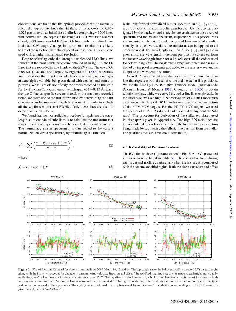
The RVs for the three nights are shown in Fig. 2. All RVs presentedin this section are listed in Table A1. There is a clear trend duringeach night and an offset, particularly when the first night is comparedwith the second and third nights. Both the slope curvature and offset

Figure 2. RVs of Proxima Centauri for observations made on 2009 March 10, 12 and 14. The top panels show the heliocentrically corrected RVs on each nightalong with the fits which account for changes in airmass, wind velocity, direction and offset. The solid/red lines indicate the fits made to each night individuallywhile the green/dashed lines are for fits made with fixed γ = 17.75. Seeing effects in the 1 arcsec slit, which varied between a maximum of 1.4 arcsec at highairmass and a minimum of 0.6 arcsec at low airmass, were not accounted for during the modelling. The residuals are plotted in the bottom panels (line typeand colour correspond to the top panels). The nightly subtracted residuals vary between 4.16 and 5.84 m s−1, while the corresponding γ = 17.75 fit residualsgive rms values of 5.56–7.43 m s−1.

MNRAS 439, 3094–3113 (2014)

at Universidad de C



Dow

nloaded from



change from night to night. We have used the empirical procedureoutlined in Figueira et al. (2010) to model the trends seen in theRVs on each night. The RV correction

� = α

(1

sin(θ )− 1

)+ βcos(θ )cos(φ − δ) + γ (4)

was shown to be sufficient to adequately remove atmospheric ef-fects. The parameters α, β, γ and δ can be determined when ob-servations are made throughout the night at the telescope elevations(θ ) and azimuth angles (φ) of a fixed target. α represents the linearRV drift per airmass (1/sin(θ )) due to changes in the line shape asdifferent layers of the atmosphere are sampled. β is effectively thewind speed at the time of the observation and δ is the wind direction.γ is an additional offset term that describes the offset of the obser-vations from zero, when all other terms are zero; in our case, thisis the heliocentric velocity correction. We have enabled all parame-ters to be fitted in order to optimize the fit for each individual night.After subtracting the nightly fits, the residuals yield rms values ofσ = 4.16, 5.50 and 5.84 m s−1 on each of 2009 March 10, 12 and14, respectively (Fig. 2). See also Table A1 for a list of all correctedvelocities (column 4, titled ‘I corr’). These values appear reasonableconsidering the expected Poisson-limited S/N of ∼2 m s−1 (Barneset al. 2013). From previously unpublished archival HARPS data3

and UVES observations (Zechmeister et al. 2009), we find the RV ofProxima Centauri to show rms scatter at the 2.3 m s−1 (27 observa-tions) and 4.3 m s−1 (339 observations) levels, respectively (Tuomiet al., in preparation).

The typical wind speed values we determine (130, 150 and190 m s−1 for each night) are large and potentially not physicallyrealistic. In addition, we find respective values for α, the variationper airmass, of 31, 11 and 23 m s−1 while the value of γ varies be-tween −169.1 and 100.9 m s−1 (i.e. 270 m s−1 variation). As notedby Figueira et al. (2010), γ and α should be fixed. However, the ob-servations are not ideal, with varying humidity [see Gray & Brown(2006) for a discussion of temperature, pressure and humidity ef-fects, which can reach km s−1 levels]. The additional problems withthe cyclical behaviour during good seeing and the apparent trendof uncorrected RV drift with seeing, especially when the seeingFWHM falls in the 0.6–0.8 arcsec range in the 1 arcsec slit, arelikely to yield systematics. For this reason, we believe that thedata are not able to reliably constrain wind speed values and di-rections for the Proxima Centauri observations, unlike the highlystabilized HARPS observations of τ Ceti. Nevertheless, by holdingγ fixed at the mean velocity (for the three nights) and fixing the17.75 m s−1 value for α found by Figueira et al. (2010), the corre-sponding corrected RV rms values for each night are σ = 6.00, 5.60and 7.43 m s−1 on March 10, 12 and 14, respectively. The correctedvelocities using this procedure are listed in Table A1 (column 5, ti-tled ‘A corr’). More reasonable wind speeds of 115, 74 and 53 m s−1

are found, but again we stress that these are probably biased by theunconstrained effects discussed above. Most notably, the curvatureis not fitted well in these fits (Fig. 2, green curves in the upper panel)indicating the probable involvement of seeing variations. For com-parison, when considering the data taken with an airmass range upto 1.5, Figueira et al. (2010) found rms scatter of between 4.54 and5.81 m s−1 for τ Ceti (G8.5V) using the same method as describedhere. The RV of τ Ceti is known to be very stable with a standarddeviation of 1.7 m s−1 (Pepe et al. 2011).

3 http//archive.eso.org/eso/eso_archive_main.html

4.4 Concluding remarks

The study in this section was motivated by a desire to characterize asimultaneous reference fiducial in order to obtain a local wavelengthsolution for our deconvolution procedure. With a few caveats, weare able to reproduce similar precision with an M6V star (ProximaCentauri) to that achieved with a G8V star (τ Ceti) with HARPS.Undoubtedly, a stabilized spectrograph, a narrower slit (or at leasta slit width well matched with the median seeing) should removesome of the additional trends in the data that equation (4) cannot de-scribe. Despite these promising findings, the major drawback of thisprocedure is that regular observations of a single target throughouteach night would be necessary for successful implementation. Wewould never realistically expect to observe a given target at sucha range of airmasses, and indeed Figueira et al. (2010) found thatrestricting observations to a narrower airmass range was necessaryto achieve the precisions reported.

Given that the trends throughout each night are also approxi-mately linear or quadratic, correcting for atmospheric effects witha four-parameter fit such as equation (4) clearly requires very highS/N ratio. Obtaining few m s−1 precision via this method has beenpossible for Proxima Centauri observations that enable S/N ratiosof a few hundred. However, typical observations of late M stars willonly achieve S/N ratios of several tens, which will more severelyrestrict the precision achievable. Internal calibration references aretherefore always a preferred and more realistic option for obtainingthe local wavelength solution for deconvolution. We thus subse-quently adopt this procedure for our ROPS sample of late M dwarfs,described in the following sections.

5 UVES O BSERVATI ONS O F A LATEM DWARF SAMPLE

For the late M stars observed with UVES, our strategy comprised ofobserving the same sequence of 15 targets during each of four halfnights. The observations were made over a 6 d period on 2012 July23, 24, 26 and 29. This enables a time span that is sufficient to discernshort-period signals of the order of a few days. Since we are unableto implement the procedure described in the previous section, whichmade use of the telluric lines to update the wavelength solution fordeconvolution of each spectrum (see Section 4.4), we used the near-simultaneous ThAr frame recorded after each observation as a localwavelength solution.

5.1 RV stability of UVES

In B12, we determined an incremental drift relative to a referencewavelength solution in order to obtain the local wavelength solutionin each order. The MIKE spectrograph however exhibited shifts ofup to a few hundred m s−1 over short time-scales, which we at-tributed to mechanical stability and possible gravitational settlingof the dewar as the coolant boils off during the night. UVES appearsto exhibit a much more predictable behaviour in that a more mono-tonic drift in wavelength is seen through a single night, althoughthere is an offset between each night as shown in Fig. 3 (top panels).Again the nightly offset may be related to both dewar refills andto re-configuration of UVES which regularly observes at differentwavelengths. Shifts of the order of 50 m s−1 can be expected withUVES when different ThAr spectra are taken after changing the

MNRAS 439, 3094–3113 (2014)

at Universidad de C



Dow

nloaded from



Figure 3. Stability of UVES during observations in 2012 July. The top panels show the drift in m s−1 on each night and the middle panels plot the temperatureof the red camera. While 0.◦4–0.◦6 drift is seen on each night, the absolute temperature values are different. The bottom panels show the drift versus thetemperature. Temperatures are plotted as filled red circles (scales on the left and bottom axes), while pressure is plotted as filled green squares (scale in hPa onthe right and top axes).

instrument configuration.4 In addition, shifts of the order of1/20 pixel per 1 hPa (millibar) change in pressure and the sameshifts for a change of 0.◦3 in temperature are typical. The recorded0.◦4–0.◦6 variation throughout each night (Fig. 1, filled red cir-cles) during our observations would thus lead us to expect a 100–150 m s−1 wavelength shift. The pressure drift on each night is of theorder of 1 hPa (Fig. 1, filled green squares) and hence presumablycontributed to the observed drift. While attributing the observedshifts to temperature changes alone is in agreement with expecta-tion on nights 2, 3 and 4 of our observations, the first night, whichwas the least humid, showed ∼400 m s−1 drift through the night. Atthe same time, the temperatures were highest on the first night, pos-sibly indicating that drift rate is correlated with temperature. Thisincreased drift rate is discussed later in light of our derived RVs.

5.2 Local ThAr wavelength solution

Subsequent to obtaining a master solution for each star, as out-lined in Section 3.1, we have adopted a method for obtaining thelocal wavelength solution for each frame that is different from thatdescribed in Section 4.2, which made use of telluric lines. Forour ROPS targets, we obtain the local wavelength frame taken af-ter each observation by instead updating the wavelength positionsof all the ThAr lines used to determine the master solution. Thepixel positions of all the lines are calculated as outlined in Sec-tion 3 before subtracting the line positions of the master wave-length frame. This procedure has the advantage that lower ordercorrections can then be applied to update the master wavelengthsolution. A two-dimensional fit is made for pixel position versus or-der for all the measured pixels. In other words, a two-dimensionalpixel shift surface is determined and we find that a polynomial of

4 http://www.eso.org/sci/facilities/paranal/instruments/uves/doc

Figure 4. Example of the ThAr line pixel shifts for EEV (blue circles)and MITLL (red squares) CCDs for the 33 extracted orders. The black ‘+’symbols represent the fitted 3 (wavelength) by 2 (cross-dispersion/order)polynomial surface. Shifts are relative to the master wavelength frame takenwith each observation on the second night of observations.

degree 3 (quadratic) in the wavelength direction and 2 (linear) inthe cross-dispersion direction (Fig. 4) is sufficient to describe thedrifting wavelength solution relative to the master solution whichwas calculated via a 4 × 6 polynomial (Section 3.1). The fitted pixelshift surface can be written as

�p(x, y) =2∑

i=0

aixi

1∑j=0

bjyj , (5)

where �p(x, y) is the pixel drift surface defined at each pixel, x,and extracted order number, y. The coefficients a and b scale the xand y terms of power i and j, respectively. The pixel surfaces areconverted to an updated wavelength surface by calculating wave-length increments from the master wavelength frame and adding tothe master wavelength frame. This procedure has the advantage ofmaintaining stability as any order edge effects are minimized in a

MNRAS 439, 3094–3113 (2014)

at Universidad de C



Dow

nloaded from

http://www.eso.org/sci/facilities/paranal/instruments/uves/doc



low-order fit. Zero-point rms values in the wavelength solutions of2.01 ± 0.20 and 2.63 ± 0.24 m s−1 for the EEV and MITLL chips,respectively, are found. As already noted in Section 3, these valuescould be reduced by using additional calibration lamps, but we notethat the 1σ variability is an order of magnitude lower at 20 and24 cm s−1, and well below the photon-noise precision that can beachieved with UVES using the techniques described in this paper.

5.3 RVs of 15 late M dwarfs

The mean-subtracted RVs for our ROPS targets are plotted in Fig. 5with details of rms estimates listed in Table 1. Appendix A gives fulldetails of all RVs, which are listed in Tables A2 and A3. The RVsare measured as outlined in B12 by subtracting the deconvolvedtelluric line position from the simultaneously observed stellar line.The line positions are measured by cross-correlating each stellarline relative to the mean deconvolved stellar line for each target,and similarly for the telluric lines. We use the HCROSS algorithm ofHeavens (1993) which is a modification of the Tonry & Davis (1979)cross-correlation algorithm. HCROSS utilizes the theory of peaks inGaussian noise to determine uncertainties in the cross-correlationpeak. We have made a minor modification of the routine, whichbelongs to the Starlink package, FIGARO, in order to directly outputboth the pixel shift and shift uncertainty.

From Table 1, it can be seen that a range of exposure timesand S/N values were obtained, depending on the brightness of thetarget, which ranged from mI = 9.5 to 14.1. In addition, not allobserved targets possess slow rotation, which we define as at orbelow the instrumental resolution of 54 000 or 5.55 km s−1. Jenkinset al. (2009) found that M6V stars possess v sin i = 8 km s−1 onaverage, while this increases to ∼15 km s−1 for M9V. Table 1 andFig. 5 demonstrate that those stars with slower v sin i values on thewhole appear to enable better RV precision to be determined, asfirst noted by Butler et al. (1996). This is not surprising since theresolution is effectively degraded and line blending increases withincreasing v sin i. The correlation between photon-limited precisionand rms for a given v sin i was also simulated in B12 and Barneset al. (2013), and we further discuss and illustrate the ‘excess’ rms(i.e. above that expected from v sin i and S/N ratio alone) in Sections5.4 and 5.5.3 and Fig. 8.

For the early M dwarf sample targeted by HARPS, Bonfils et al.(2013) found an anticorrelation when plotting bisector spans (BIS)against the measured RVs. For instance, a clear correlation (witha Pearson’s correlation of r = −0.81) was identified for Gl 388(AD Leo). Subtraction of the trend decreased the rms from 24 to14 m s−1. We have calculated the BIS (Gray 1983; Toner & Gray1988; Martınez Fiorenzano et al. 2005) for all our stars and sub-tracted the best-fitting linear trend with the derived RVs. The uncor-rected RVs are listed in column 9 of Table 1, while the BIS-correctedRVs are listed in column 10 and show that a number of our starsalso demonstrate trends that are linked with the line bisector span(BIS). These stellar line BIS-corrected velocities and subsequentrms values are plotted in Fig. 5, and we refer to these correctedvalues in the following discussion. Significant improvements in therms are seen for a number of targets, where the rms is halved. Thecorrected RVs however show little improvement in the stars thatexhibit the largest v sin i and derived rms values. Improvements arealso seen if a correlation with the telluric BIS is removed (column11), indicating that atmospheric variation may also contribute tolimiting the precision that can be achieved using the methods out-lined above. Also, variability in the slit illumination (e.g. due toseeing changes) affects the instrumental point spread function, thus

affecting both stellar and telluric lines to some degree. This will gosome way to explaining why stellar or telluric lines can improve themeasured rms. However, only the stellar lines contain line shapevariability introduced by the star itself. Finally, we have also inves-tigated incorporating both the line and telluric BIS measurements.Since the final RVs are measured by subtracting the telluric lineposition from the stellar position, we also list RV-BIS correctionsfor a stellar–telluric BIS correction (column 12).

5.4 Discussion

The rms velocities demonstrate that near-photon noise-limited pre-cision is achievable using our red-optical survey. Following B12,where photon-noise-limited simulations were made with the MIKEspectrograph at the 6.5 m Magellan Clay telescope, we have es-timated that 1.5–2 m s−1 should be achieved with UVES (Barneset al. 2013). The observations, in particular for GJ 1061, GJ 1002and 2MASS J03341218−4953322 (Table 1) thus show considerableimprovements over recent measurements that have made use of tel-luric lines as a reference fiducial (e.g. Reiners 2009; Bailey et al.2012; Rodler et al. 2012). The BIS-corrected 2.4, 5.1 and 6.4 m s−1

measurements for these objects compare favourably with those thatwe obtained with HARPS for the brightest targets in our sample.While GJ 1061 and GJ 1002 have not been actively monitored withHARPS, four observations for each target (that remain unpublished)exist in the ESO’s archive. Using TERRA, the Template-EnhancedRadial velocity Re-analysis Application (Anglada-Escude & Butler2012), a pipeline suite designed to improve the RVs achieved bythe standard HARPS Data Reduction Software, we have found 2.04and 2.32 m s−1 precisions for GJ 1061 and GJ 1002 (see Table A4for RVs). We note that only the reddest orders of HARPS in thevery brightest mid-M targets enable precision of a few m s−1 to beachieved.

Despite the sub-10 m s−1 rms values, a number of our stars exhibitRVs that are significantly in excess of the photon-noise-limitedprecision that we expect from our targets, even when v sin i istaken into consideration. The RVs for the less stable targets indicatethat rotation and activity may play a role in the observed largerrms values. As the average M6V star exhibits v sin i = 8 km s−1

(Jenkins et al. 2009), we expect velocity precisions of ∼10 m s−1 forS/N = 30 (Barnes et al. 2013). However, while we predict photon-noise-limited precisions of 13, 15 and 20 m s−1 for GJ 3076, LP759-25 and LP 412-31, respectively, they exhibit RVs that are anorder of magnitude higher. The uncorrected RV values for thesetargets are also not significantly improved (at least relative to thephoton-limited precision) when we include BIS corrections with thestellar lines or telluric lines. The best improvement is seen for thecombined stellar and telluric line correction. While it is possible toselect stellar lines for deconvolution that are free of any significanttelluric lines (i.e. we use regions free of telluric lines with depths>0.05 of the normalized continuum), it is conversely not possibleto select telluric line regions that are free of stellar lines. Any cross-contamination of the tellurics is thus more likely if the stellar linesshow signs of activity variability. To ascertain whether the increasedrms scatter may be related to stellar variability, in Section 5.5 weinvestigate spectral lines that are sensitive to chromospheric activity.

5.4.1 The effect of instrumental drift on RV precision

The first night of our observations, 2012 July 23, was particularlydry and hence tellurics with smaller equivalent widths (EWs) were

MNRAS 439, 3094–3113 (2014)

at Universidad de C



Dow

nloaded from



Figure 5. Heliocentrically corrected RVs plotted for our 15 UVES ROPS targets. Observations were made on 2012 July 22, 23, 25 and 28. The sample containsa total of seven M5V–M6.5V and eight M7V–M9V targets. An RV precision of 2.4 and 5.0 m s−1 is measured for quiet, slowly rotating targets at spectral typeM5.5V (GJ 1061 and GJ 1002), while 6.4 m s−1 is found for our latest, M9V, target (2MASS J03341218−4953322). The targets showing higher rms in Table 2either exhibit significant rotation (v sin i � 10 km s−1), significant variability in the chromospheric indicators, Ca II and Hα or both.

derived, leading to RVs with larger error bars. Fig. 3 also shows thatthe largest drift rates were observed with UVES on the first night.Those targets that were observed during the highest rate of driftappear to show RV measurements with the greatest offset on eachnight. One might expect an improved velocity precision if each stel-lar observation were bracketed by ThAr observations, which would

enable interpolation of the wavelength scale to the time centroidof the observation. Applying this procedure did not significantlyimprove our rms precision however, probably because the preced-ing ThAr was taken before the telescope was slewed to the newobject. Unlike properly stabilized and fibre-fed instruments UVESis located at one of the Nasmyth foci and is thus potentially subject

MNRAS 439, 3094–3113 (2014)

at Universidad de C



Dow

nloaded from



Figure 6. The Ca II 9662.14 Å profiles (left) and corresponding Hα (6552.80 Å) lines (right) for all observations of the 15 ROPS targets listed in Table 1. Foreach target, the matched colour is used to signify that the Ca II 9662.14 Å and Hα lines were extracted from the same spectrum. We have also included profilesfrom the Proxima Centauri data set for the minimum, maximum and mean Hα emission and corresponding Ca II 8662.14 Å levels. The plotted wavelengthsspan 4 Å for Ca II and 6 Å for Hα. The blending of the Ca II 8662.14 Å profile with the nearby Fe I line at 8661.90 Å is clearly seen in the slower rotating, earlierstars in the sample (e.g. GJ 1002, GJ 1061 and GJ 3128). 2MASS J03341218−4953322 possesses a large RV (see Appendix A, �2M J03-49 = 73 732.21 m s−1),and since the Ca II line is located near the edge of the order, the spectrum appears truncated when the line is re-centred to 8662.14 Å.

to vibration and centripetal forces through slewing of the telescopefrom one target to the next. It is not clear whether movement ofthe telescope is able to affect the drift rate, but it does not nec-essarily appear to result in random changes in the drift direction.Bracketing every science exposure with ThAr exposures (i.e. im-mediately before and after the observation), with the telescope atfixed Right Ascension and Declination, is likely to enable furtherimprovements in RV precision. This procedure will be adopted withany future observations.

5.5 Chromospheric activity

The degree of stellar variability, as measured from chromosphericactivity indicators in our target sample, varies considerably. Whilesome of our more RV-stable targets such as GJ 1061 and GJ 1002show low levels of chromospheric activity (e.g. flaring), others at

similar spectral type and activity levels, such as Proxima Centauri,show higher levels of variability in lines such as Hα. The degree towhich chromospheric activity significantly impacts upon measuredRVs is not well known for mid-to-late M dwarfs. Reiners (2009)found that the flaring activity, with 0.4 dex variability in Hα for themid-M star, CN Leo, did not result in RV deviations at the 10 m s−1

level, although a large flare event in that study did result in an RVdeviation of several hundred m s−1. The impact and correlation ofactivity variability with measured RVs in our ROPS sample areinvestigated in the following sections.

5.5.1 Hα as an activity indicator

In order to monitor the chromospheric activity of each star (i.e.presence of active regions and flaring events), we have examinedthe Hα line, which is plotted for all observations in Fig. 6 (the

MNRAS 439, 3094–3113 (2014)

at Universidad de C



Dow

nloaded from



Ca II 8662.14 Å line, also plotted, is discussed in Section 5.5.4).In the case of Proxima Centauri, we plot the minimum, mean andmaximum Hα emission since there are a total of 561 observationsin the 2009 data set.

We have estimated the activity in our ROPS sample, by calcu-lating Hα emission for all observations of each target. The Hα

emission in each spectrum was calculated by measuring the EW ofthe line. We adopted the procedure described in West et al. (2004),by measuring the EW(Hα) relative to the normalized continuum.Following West & Hawley (2008), the continuum regions are de-fined as 6555–6560 and 6570–6575 Å. Several of our targets, GJ1061, GJ 1002 and GJ 3128, have some or all measurements thatyield negative EWs since the local continuum level is difficult tomeasure when Hα is barely visible. We have therefore assumed thatall measurements are relative to the lowest measured EW whichwe assume is limited by the calculated EW uncertainty, as mea-sured from the variances propagated during extraction. For any starwith a significant emission EW, this uncertainty is negligible. Us-ing flux-calibrated spectra from nearby M stars, West & Hawley(2008) estimate χ values, the ratios of continuum flux around Hα

to the bolometric flux. Using their tabulated values of χ for Hα, wecan determine FHα/Fbol = LHα/Lbol = χ (Hα) EW(Hα). The sameprocedure was adopted by Mohanty & Basri (2003) who instead ofusing flux-calibrated observations relied upon the models of Allardet al. (2001) to estimate χ . Luminosities are presented in the form,log10(LHα/Lbol), which are given for each star in Table 2. It is im-mediately evident that the majority of stars show some degree ofvariability. Visual representations of the Hα variability as a functionof both spectral type and v sin i are shown in Fig. 7.

For the most stable star in the sample, GJ 1061, Hα is barelydiscernible, with variability of ∼4 per cent of the normalized con-tinuum. Both GJ 1002 and GJ 3128 show Hα that is also filled inbut with variability at the 20 per cent level. On the other hand, theM6.5V to M9 targets all show Hα in emission that varies consid-erably (see values in Table 2). The notable targets, however, arethose exhibiting significant rotation, with Hα in strong emission,namely LP 412-31, GJ 3146, LP 759-25 and GJ 3076. These tar-gets possess the highest rotation in our sample, with v sin i valuesof 12, 12.4, 13 and 17.1 km s−1 respectively. GJ 3076 shows theleast variability, indicative of saturation, while LP 412-31 (with thehighest measured EW) is also only moderately variable. Bell et al.(2012) also made this observation for the complete M spectral range(M0V–M9V). They attributed this phenomenon to the higher levelof persistent emission requiring significant heating (flaring) eventsto give a measurable change in emission.

Mohanty & Basri (2003), West et al. (2004) and more recentlyReiners & Basri (2009, 2010) have studied rotation and activityacross the M dwarf spectral class. By observing large samples, thesestudies indicated trends with chromospheric activity and v sin i.West et al. (2004) studied 8000 spectra of low-mass stars from theSloan Digital Sky Survey and found that 64–73 per cent of M7V–M8V stars were active. Here, although our sample is small, wesee considerable variability in any specific object. Hence, for themore active targets, a single snapshot observation is not necessarilyrepresentative of the mean activity level for that particular star. Thetrend first noted by Mohanty & Basri (2003) and further quantifiedin Reiners & Basri (2010) suggests that Hα emission occurs at lowerrotation rates in the later M stars. This is also apparent in our sample,where the M5V–M6V targets with slow rotation ≤5 km s−1do not onthe whole show a strong Hα line, whereas the M6.5V–M8V targetsall possess significant Hα emission and variability for the similarrotation velocities. The sudden fall in LHα/Lbol noted by Mohanty

Figure 7. Activity, log10(LHα /Lbol), as a function of spectral type (top) andv sin i (bottom) for the 15 ROPS targets and Proxima Centauri. The symbolsand colours for each object are indicated in the lower panel key and applyto both plots. The earliest star with significant rotation exhibits the highestlog10(LHα /Lbol), while down to M8V, significant activity variation is seenat more moderate rotation speeds. Except for Proxima Centauri, the slowlyrotating M5.5V–M6V stars show little Hα activity, while the latest stars inthe sample (M8.5V and M9V) are also less active.

& Basri (2003) is seen in our latest targets, which despite similarrotation velocities of 6 and 8 km s−1 show both the smallest EWHα

and log10(LHα/Lbol) values. Our findings are thus in keeping withthe late spectral type activity frequency plots of Reiners & Basri(2010) (see their fig. 7).

5.5.2 Morphology of Hα emission line

We make an additional observation regarding the shape of the Hα

line, which may be applicable to stars (or subset populations ofstars), such as the latest M dwarfs, where Hα is always seen inemission. The exact morphology of the line appears to vary, withthe emission profiles for some objects appearing to exhibit morepronounced double-horned peaks than others. Further investigationof the detailed shape of Hα is warranted when it is realized thatthis shape is typical of emission from time-varying circumstellarmaterial at high stellar latitude. For example, Barnes et al. (2001)observed variability of Hα emission in the low axial inclinationG8V α Persei star AP 149, attributing it to a prominence system. ADoppler tomogram, derived using the code developed by Marsh &Horne (1988), enabled four main emitting regions, located at andbeyond co-rotation, to be inferred. While this technique requires

MNRAS 439, 3094–3113 (2014)

at Universidad de C



Dow

nloaded from



Table 2. Hα variability for each object. Minimum and maximum Hα equivalent widths are listed foreach object in columns 4 and 5, respectively. The corresponding minimum and maximum log10(LHα /Lbol)are calculated from the appropriate models and listed in columns 6 and 7 (see Section 5.5.1).

Star SpT v sin i Min Max Min Max(km s−1) EW (Å) EW (Å) log10(LHα /Lbol) log10(LHα /Lbol)

GJ 3076 M5V 17.1 5.59 6.36 −3.81 −3.76GJ 1002 M5.5V ≤3 0.01 0.17 −6.51 −5.42GJ 1061 M5.5V ≤5 0.01 0.03 −6.74 −6.12LP 759-25 M5.5V 13 2.48 7.27 −4.08 −3.79GJ 3146 M5.5V 12.4 2.80 3.92 −4.20 −4.05GJ 3128 M6V ≤5 0.02 0.13 −6.36 −5.62Proxima Centauri M6V 2 0.56 2.11 −5.00 −4.43GJ 4281 M6.5V 7 0.85 1.06 −5.01 −4.92SO J0253+1652 M7V ≤5 0.21 0.51 −5.61 −5.58LP 888-18 M7.5V ≤3 2.65 4.51 −4.83 −4.60LHS 132 M8V ≤5 7.25 12.09 −4.36 −4.142M J2306−0502 M8V 6 2.34 4.17 −4.85 −4.60LHS 1367 M8V ≤5 2.59 6.11 −4.81 −4.44LP 412-31 M8V 12 19.72 21.11 −3.93 −3.902M J2331−27495 M8.5V 6 1.53 2.02 −5.12 −5.012M J0334−49533 M9V 8 0.19 1.08 −6.14 −5.39

sufficient velocity resolution to enable such a study, asymmetricvariability of Hα emission may well be measurable in more slowlyrotating stars. We find such variability at the 1–2 per cent levelin the Proxima Centauri observations, with a trend suggesting aperiod that is greater than the 5 d time-scale of the observations.With prolonged monitoring, the rotation period of stars that showHα in strong emission may thus be estimated, while the exact shapeof the emission (the prominence of the horns) may change withinclination angle.

5.5.3 Hα and v sin i as a proxies for RV precision in late M stars

The upper panel of Fig. 8 shows a plot of v sin i versus rms (stellarline-corrected BIS) values in this paper, illustrating the importanceof v sin i in limiting the attainable precision as might intuitively beexpected. We note that 2MASS J03341218−4953322 attains a pre-cision that is greater than photon statistics predict (i.e. lower rms).This is probably a statistical effect that could potentially affect anysmall sample of observations. The contours plotted in Fig. 8 wereestimated by Barnes et al. (2013) using Monte Carlo simulationswith an M6V model atmosphere (Brott & Hauschildt 2005), whilethe increased number of opacities in an M9V star would lead us toexpect a lower achievable precision. The Pearson correlation coef-ficient, r, gives an indication of the correlation. For v sin i versusrms, we find r = 0.74, indicating a strong positive correlation. Theslope of the correlation itself is important when using v sin i as anindicator of expected precision. The discrepancy from the photon-noise-limited precision is greatest for the stars with the highestv sin i values, as we noted for the most rapid rotators in Section 5.4.Relying on v sin i to obtain an estimate of rms may therefore leadto an underestimation of the stellar jitter.

In Fig. 8 (middle panel), the spectral type versus rms is plotted.Clearly, the correlation with spectral type is weak, where we findr = 0.04. If we instead consider log10(LHα/Lbol) as an indicatorof rms, as plotted in Fig. 8 (bottom panel), we again see a cleartrend. The Pearson correlation coefficients for the lower and upperlog10(LHα/Lbol) values are r = 0.76 and 0.82, respectively. Consider-ing upper and lower limits together, we obtain r = 0.77. The signif-icance of the trend of v sin i versus rms and that of log10(LHα/Lbol)

versus rms across our sample are thus comparable. It would ap-pear that the absorption lines of late-type stars are significantlyaffected by magnetic activity, especially when moderate rotationof v sin i ∼ 10 km s−1 and above is observed. Although relying onv sin i to estimate rms may underestimate the jitter in this regime, theuse of Hα emission level instead removes the rotation dependence.

5.5.4 Ca II 8662 Å activity and correlation with Hα variability

The Ca II H&K lines have regularly been monitored in F-M-typestars for many years (e.g. Wilson 1978; Baliunas et al. 1995) sincetheir emission cores show strong variability connected with stellarmagnetic activity. The S index measured from the H&K lines (Bal-iunas et al. 1995) is known to be a general indicator of activity as itis related to the area and the strength of magnetic activity on a star(Schrijver et al. 1989). Stars with low log R′

HK indices (the fractionof a star’s luminosity in the Ca II H&K lines) are generally selectedfor precision RV searches for planets (e.g. Wright et al. 2004). Therole of Ca II H&K excess emission and its relationship with jitter inthe large sample of the California Planet Search have been studiedby Isaacson & Fischer (2010) for instance. In the subset of theirsample that includes the latest stars (early M dwarfs), a noise flooris seen with evidence for a trend that increases with activity, asdiscussed in Section 5.5.3 above.

Although the Ca II H&K lines are very strong and easily accessi-ble for F-K-type stars observed with most high resolution spectrom-eters, the flux at blue wavelengths, especially by mid-M spectraltype, is too low to enable sufficient S/N to be attained during typicalobservations. Other Ca II lines that are sensitive to chromosphericactivity, such as the so-called infrared Ca II triplet, are howeverobserved in the wavelength regime in which our survey operates.Of the infrared Ca II triplet lines at 8498, 8542 and 8662 Å, thelatter line appears the least blended. Hence, we chose to illustratethe non-local thermodynamic equilibrium behaviour (i.e. potentialemission in the core) of this line in Fig. 6. The line becomes indis-tinct, through blending with other lines, in the later spectral types inour sample. In our ROPS sample, variability above the noise levelcan be discerned in Fig. 6, notably for GJ 3076 and LP 412-31.The clearest variation in this line is seen with LP 759-25 (similar

MNRAS 439, 3094–3113 (2014)

at Universidad de C



Dow

nloaded from



Figure 8. Key stellar parameters plotted against rms (line BIS corrected)for the ROPS targets and Proxima Centauri. The plots are of v sin i versusrms (top), spectral type versus rms (middle) and activity (log10(LHα /Lbol))versus rms (bottom). The symbols and colours used in all panels denote theS/N ratios or S/N ratio intervals for each observed target: 0 ≤ S/N < 15 (redsquares), 15 ≤ S/N < 30 (green circles), 30 ≤ S/N < 60 (blue triangles),S/N ≥ 100 (magenta diamonds). Similarly, photon-noise-limited contoursfrom Barnes et al. (2013) are plotted in the top panel for S/N = 15, 30,60 and 120, respectively (red/solid, green/long-dash, blue/short-dash, ma-genta/dotted). The stars with the highest v sin i values are most discrepantfrom the photon-noise-limited case, indicating the importance of activity asan indicator of expected precision. Maximum and minimum values of Hα

luminosity, as given in Table 2, are plotted as circles connected by a line foreach star in the bottom panel. For GJ 1061, 1002 and 3128, very small lineEWs were found for some or all (GJ 1061) phases. An arrow head indicatesthat the lowest Hα luminosity is a sensitivity limit, and equal to the EWuncertainty.

variability is also seen, but not plotted, in the other two infraredCa II lines).

It appears that variability in the Ca II 8662 Å line is only easily dis-cerned for very strong flares. Fuhrmeister, Liefke & Schmitt (2007)observed the behaviour of the Ca II triplet lines for the flaring M5.5dwarf CN Leo, noting the correlation with other chromosphericlines. In the case of Proxima Centauri, Fuhrmeister et al. (2011)presented UVES observations of Ca II H&K, Hα alongside opticallight curves (obtained with the blue exposure meter of UVES). TheCa II triplet lines were not discussed in their study; however, simul-taneous observations with XMM–Newton, covering the 0.2–10 keVrange and the U band (300–390 nm), were presented. We have alsoincluded Hα and Ca II 8662 Å in Fig. 6 to demonstrate the range

of variability seen over all observations of the 2009 data. Profilesare included for the minimum, mean and maximum states, with thelatter corresponding to the strongest flaring event on the final night.Although the correlation between Hα variability and the infraredCa II triplet variability was not included in the study by Fuhrmeisteret al. (2011), their figs 1–3 showed a strong correlation betweenHα and Ca II H&K (albeit at a lower observation cadence neces-sitated by the longer exposure times required in the blue arm ofUVES with an M6V star). Since the infrared Ca II triplet lines areheavily blended, we have determined the variability in Ca II 8662 Åby subtracting the mean spectrum (derived from all observations).The relative EW was then measured for each observation. We findthat the correlation between Hα and Ca II 8662 Å EW values isvery strong, with Pearson correlation coefficients of r = 0.92, 0.94and 0.91 for each of the three nights. The Ca II triplet lines are thuspotentially useful for identifying strong flaring events, although thestrength of Hα makes it the more useful line for activity monitoringin the first instance.

5.5.5 Selection of RVs based on activity events

A very large flare was observed during the observations of CN Leo(Reiners 2009) that lead to 660 m s−1 deviation from the other RVsthat were measured with ∼10 m s−1 precision. For all other flareevents resulting in log10(LHα/Lbol) changes of ≤0.4 dex, Reiners(2009) found no RV variability at the 10 m s−1 precision of theobservations. The conclusion from that study is that only the verystrongest flares, which are easily identifiable in spectra, affect RVsat the level of ∼500 m s−1. The large flare on Proxima Centauri on2009 March 14 resulted in a change of Hα emission of 0.33 dex(comparing the immediate pre-flare and maximum flare EWs). Ourrms precision on 2009 March 14 was 5.84 m s−1 (full four-parametercorrection). However, excursions of up to 20 m s−1 can occasionallybe seen in the bottom panels of Fig. 2 that do not necessarily coincidewith the flaring events presented in Fuhrmeister et al. (2011). Beforeand after the sudden rise in Hα emission corresponding to the largeflare on 2009 March 14, the RVs appear to be relatively stable(Fig. 2, bottom-right panel) in the t ∼ 4.23–4.25 d and 4.28–4.30 dregions. However, from t ∼ 4.26–4.28 d, there is systematic RVdeviation of ∼20 m s−1 coinciding with the onset and peak of theflare. It is difficult to determine whether the flare is responsible sincesystematic deviations of similar magnitude occur on 2009 March12 and earlier on 2009 March 14. No strong flare counterpart isseen in the other activity indicators presented in Fuhrmeister et al.(2011) for these RV deviations. The correlation coefficient betweenHα EWs and RVs for the complete Proxima Centauri data set isr = −0.09. For the region where Hα EW increases and the RVsshow the tentative peak (t = 4.255–4.276 d), r = −0.28, indicatinga weak negative correlation. The behaviour of Hα is more complexhowever during this strong flare cascade. Fig. 3 in Fuhrmeister et al.(2011) shows that the Hε and H I 3770 Å lines exhibit a more clearlydefined peak (i.e. a sharper decline after the sharp rise at XMM—Newton wavelengths) that may indicate a higher correlation withthe RVs. In conclusion, it is not clear that the strong flare reallyimpacted on our RVs in this case and there is no evidence that anyof the other flare events affected the RVs on Proxima Centauri atthe 4–6 m s−1 level during the three nights of the observations.

Although the evidence suggests that moderate flaring does notaffect RV measurements at ≥10 m s−1 on slow rotators, it is notclear whether this is also true for moderate rotators. In this instance,activity-related transients might be more clearly resolved owing toDoppler broadening of the lines. If we remove the observation

MNRAS 439, 3094–3113 (2014)

at Universidad de C



Dow

nloaded from



of LP 759-25 (v sin i = 13.7 km s−1), which shows Hα in strongemission and evidence for a large flare (in both Hα and Ca II 8662 Å),the measured rms reduces from 79.9 km s−1 (line bisector corrected)to 29.7 km s−1. While this represents a dramatic improvement, and isnow twice our predicted photon-noise-limited precision of 15 m s−1

(see earlier discussion in this section), it is difficult to determine thesignificance given that the rms values are based on only four andthree observations alone, respectively.

It is thus clear that more observations are needed for each starbecause if late M stars are moderate rotators on average that showmodulated activity, then measuring precise RVs at the sub-10 m s−1

level will prove extremely challenging. De-trending of RVs usingactivity indicators generally utilizes of the order of 20–30 epochs,at which stage planetary signals can be well characterized (e.g.see Bonfils et al. 2013). Monitoring of activity indicators for strongflaring events in late M dwarfs is also essential. For CN Leo (Reiners2009), only ∼4 per cent of observations were affected by a strongflare. We also see very tentative evidence (with weak correlation),for RVs affected by flare activity (at the 20 m s−1 level) in ∼4 percent of the Proxima Centauri observations.

6 C O N C L U S I O N A N D F U T U R E P RO S P E C T S

With careful wavelength calibration we have demonstrated that2.4 m s−1 precision can be achieved with UVES operating in thered part of the optical. Since we have so far only obtained threeto five RV measurements per star spanning six nights, further ob-servations are required before any potential planetary signals canbe discerned. However, under the assumption that the current rmsestimates are representative of a larger set of observations, and byconsidering our most stable targets that exhibit rms < 16 m s−1,we can rule out the presence of planets with mp sin i > 10 M⊕ in0.03 au orbits. Extending this to include the less stable stars, ourobservations do not support evidence for planets more massive thanmp sin i = 0.5 MJ at 0.03 au. Fig. 9 illustrates the late M param-eter space of this investigation, presenting our ROPS targets, theearly M dwarfs and all planets detected with RVs, orbiting stars upto 2 M�. The RVs corrected with the stellar line BIS are plottedas upper limits, and at present are only intended to illustrate thesensitivities achieved with our survey.

Figure 9. The unique parameter space explored by ROPS and currentrms limits (blue filled circles with downward arrows indicating upper lim-its). Also shown are the M dwarfs with known planetary companions (redcrosses) and all known planets with RV measurements (up to 2 solar masses)and hence mp sin i determinations.

Even a modest survey, targeting relatively small numbers of Mdwarfs, leads us to expect significant numbers of low-mass planets,following the findings of recent studies (e.g. Bonfils et al. 2013;Dressing & Charbonneau 2013; Kopparapu 2013). It is vitally im-portant however that if precisions of a few m s−1 are to be obtainedin a large sample of stars, the activity must be clearly characterizedand understood. This study was motivated by the uncharted late Mdwarfs, hence our inclusion of target stars that were typical, in termsof activity and rotation. Even with the few observations presentedhere, it is clear that any future surveys must carefully select targetsthat do not bias the sample. In other words, selection of only slowlyrotating late M dwarfs might lead to observation of predominantlylow axial inclination systems (i � 90◦) that are not as favourablefor RV planet detection. For instance, if the mean axial inclinationof a stellar population is assumed to be 45◦, and if the mean v sin i isfound to be 8 km s−1 for a typical M6V (Jenkins et al. 2009), selec-tion of stars with v sin i < 5 km s−1 will lead to a sample biased to amean axial inclination of i < 26◦. The problem becomes worse foran M9V star with a typical v sin i = 15 km s−1. Here we expect thatobservation of stars with v sin i < 5 km s−1 will lead to a samplewith a mean axial inclination of i < 14◦ (i.e. very close to pole-on).Conversely, we find that significant v sin i leads to higher rms, andmost importantly that these rms values are significantly above thephoton-noise-limited precision at the observed v sin i and S/N ra-tios. Hα luminosity, log10(LHα/Lbol), shows a clear trend with rmsas discussed in Section 5.5.3 and illustrated in Fig. 8. The implica-tion that late-type stars are significantly spotted, and hence exhibittime-varying line distortions, suggests that ways of mitigating theeffects of the resulting ‘jitter’ are important for this class of stars.

In this paper, we used a standard and straightforward bisectorspan analysis to de-trend the data. Only further observations willenable this procedure to be fully validated. At the same time, a sim-ple BIS analysis is not able to properly remove any magneticallyinduced RV signatures to the photon-noise level, especially for starswith moderate rotation. We will investigate this in a future publica-tion, but our preliminary simulations indicate that the BIS analysisis optimal for a narrow range of rotation velocities. Any starspotdistributions are also an important consideration. In Barnes, Jeffers& Jones (2011) for example, we assumed the effects of randomlydistributed spots, but did not try to remove their influence on the RVjitter. It is not at all clear that random spots, resulting from a fullyconvective turbulent dynamo, are the predominant spot pattern onactive late M spectral types. By mid-M when stars become fullyconvective, there is evidence that magnetic fields become dipolar(Donati et al. 2008; Morin et al. 2008). Doppler images are onemeans of characterizing spot patterns, but photospheric brightnessimages have currently only been derived for early M stars (Barnes &Collier Cameron 2001; Barnes, James & Cameron 2004; Phan-Baoet al. 2009).

Observing strategies are also an important consideration whentrying to mitigate any starspot effects. Moulds et al. (2013) havefound that starspot jitter can largely be removed by modellingstarspot effects on the line profile. Hence, intensive spectroscopicobservations of late M targets may be necessary to enable moreeffective removal of activity signatures. Fortuitously, M6V–M9Vplanets are expected in a close orbit about their parent stars (Bon-fils et al. 2013), which as already noted lead us to expect 6–11 dorbits at the centre of the continuous HZ (Kopparapu et al. 2013).Hence, observations over week–month-long time-scales over whichstarspot groups are stable (Goulding et al. 2012) should enable goodsampling of M dwarf planet orbits while simultaneously providingthe observations that could help remove activity jitter. In addition,

MNRAS 439, 3094–3113 (2014)

at Universidad de C



Dow

nloaded from



the use of Bayesian techniques to search for low-amplitude signalsin noise enables recovery of RV signatures in only a few epochs.Indeed, we find low-amplitude signals in the HARPS early-midM dwarf sample (Tuomi et al. 2014) that indicate that RV signalsare abundant, with occurrence rates of 0.06+0.11

−0.03 for 3 ≤ mp sin i ≤10 M⊕ in 1–10 d orbits, increasing to 1.02+1.48

−0.69 for 10–100 d planets(i.e. an upper limit of greater than one planet per star). Moreover, theestimated HZ occurrence rate for 3 ≤ mp sin i ≤ 10 M⊕ is found tobe η⊕ = 0.16–0.24. By extrapolation from early M dwarf observa-tions, we expect late M dwarf planet frequencies to peak in shorterorbits, continuing the trend of semi-major axis distribution versusstellar mass noted by Currie (2009). For example, the 33 d, 0.135 auorbit (Kopparapu et al. 2013) of an HZ planet hosted by 0.3 M�early M dwarf would reduce to an 11 d, 0.045 au orbit for the sampleplanet hosted by a 0.1 M� star. Further to the above argument, thisillustrates that short observing campaigns should quickly uncoversignificant signals for surveys that enable few m s−1 precision to beattained. The search for low-mass planets orbiting the lowest massstars is thus a challenging but achievable goal with current estimatesleading us to expect a host of interesting planets in the near future.

AC K N OW L E D G E M E N T S

We would like to thank the anonymous referee for the suggestedamendments and for careful reading of the manuscript. JB grate-fully acknowledges funding through a University of Hertford-shire Research Fellowship. JSJ acknowledges funding by Fondecytthrough grant 3110004 and partial support from Centro de As-trofısica FONDAP 15010003, the GEMINI-CONICYT FUND andfrom the Comite Mixto ESO-GOBIERNO DE CHILE. SVJ ac-knowledges research funding by the Deutsche Forschungsgemein-schaft (DFG) under grant SFB 963/1, project A16. DM and PAgratefully acknowledge support by the FONDAP Center for Astro-physics 15010003, the BASAL CATA Center for Astrophysics andAssociated Technologies PFB-06 and the MILENIO Milky WayMillennium Nucleus from the Ministry of Economys ICM grantP07-021-F. AJ acknowledges support from FONDECYT project1130857, BASAL CATA PFB-06 and the Millennium Science Ini-tiative, Chilean Ministry of Economy (Millennium Institute of As-trophysics MAS and Nucleus P10-022-F). PR also acknowledgesFONDECYT project 1120299. During the course of this work, DJPand MT were supported by RoPACS, a Marie Curie Initial TrainingNetwork funded by the European Commissions Seventh FrameworkProgramme. JB, JSJ, DJP and SVJ have also received travel supportfrom RoPACS during this research. This paper includes data gath-ered with the 6.5 m Magellan Telescopes located at Las CampanasObservatory, Chile.

R E F E R E N C E S

Allard F., Hauschildt P. H., Alexander D. R., Tamanai A., Schweitzer A.,2001, ApJ, 556, 357

Anglada-Escude G., Butler R. P., 2012, ApJ, 200, 15Bailey J. I. III, White R. J., Blake C. H., Charbonneau D., Barman T. S.,

Tanner A. M., Torres G., 2012, ApJ, 749, 16Baliunas S. et al., 1995, ApJ, 438, 269Barber R. J., Tennyson J., Harris G. J., Tolchenov R. N., 2006, MNRAS,

368, 1087Barnes J. R., Collier Cameron A., 2001, MNRAS, 326, 950Barnes J. R., Collier Cameron A., James D. J., Steeghs D., 2001, MNRAS,

326, 1057Barnes J. R., James D. J., Cameron A. C., 2004, MNRAS, 352, 589

Barnes J. R., Barman T. S., Prato L., Segransan D., Jones H. R. A., LeighC. J., Collier Cameron A., Pinfield D. J., 2007, MNRAS, 382, 473

Barnes J. R., Jeffers S. V., Jones H. R. A., 2011, MNRAS, 412, 1599Barnes J. R. et al., 2012, MNRAS, 424, 591 (B12)Barnes J. R. et al., 2013, in Saglia R., ed., European Physical Journal Web

of Conferences, Vol. 47, Hot Planets and Cool Stars. EDP Sciences, LesUlis, p. 5002

Bean J. L., Seifahrt A., Hartman H., Nilsson H., Wiedemann G., Reiners A.,Dreizler S., Henry T. J., 2010, ApJ, 713, 410

Bell K. J., Hilton E. J., Davenport J. R. A., Hilton E. J., Davenport J. R. A.,Hawley S. L., West A. A., Rogel A. B., 2012, PASP, 124, 14

Bonfils X. et al., 2013, A&A, 549, A109Borucki W. J. et al., 2011, ApJ, 736, 19Brott I., Hauschildt P. H., 2005, in Turon C., O’Flaherty K. S., Perryman

M. A. C., eds, ESA Special Publication, Vol. 576, The Three-Dimensional Universe with Gaia. ESA, Noordwijk, p. 565

Butler R. P., Marcy G. W., Williams E., McCarthy C., Dosanjh P., VogtS. S., 1996, PASP, 108, 500

Clough S. A., Iacono M. J., Moncet J. L., 1992, J. Geophys. Res., 97, 15761Clough S. A., Shephard M. W., Mlawer E. J., Delamere J. S., Iacono M. J.,

Cady-Pereira K., Boukabara S., Brown P. D., 2005, J. Quant. Spectrosc.Radiat. Transfer, 91, 233

Currie T., 2009, ApJ, 694, L171Delfosse X., Forveille T., Mayor M., Perrier C., Naef D., Queloz D., 1998,

A&A, 338, L67Donati J. et al., 2008, MNRAS, 390, 545Dressing C. D., Charbonneau D., 2013, ApJ, 767, 95Endl M., Kurster M., 2008, A&A, 488, 1149Fabrycky D. C. et al., 2012, ApJ, 750, 114Figueira P., Pepe F., Lovis C., Mayor M., 2010, A&A, 515, A106Fuhrmeister B., Liefke C., Schmitt J. H. M. M., 2007, A&A, 468, 221Fuhrmeister B., Lalitha S., Poppenhaeger K., Rudolf N., Liefke C., Reiners

A., Schmitt J. H. M. M., Ness J.-U., 2011, A&A, 534, A133Gerstenkorn S., Luc P., 1978, Atlas DU spectre d’absorption de la molecule

d’iode 14800-20000 cm-1 (Paris: Editions du Centre National de laRecherche Scientifique (CNRS), 1978)

Goulding N. T. et al., 2012, MNRAS, 427, 3358Gray D. F., 1983, in Stenflo J. O., ed., Proc. IAU Symp. 102, Solar and

Stellar Magnetic Fields: Origins and Coronal Effects. Reidel, Dordrecht,p. 461

Gray D. F., Brown K. I. T., 2006, PASP, 118, 399Griffin R., Griffin R., 1973, MNRAS, 162, 243Heavens A. F., 1993, MNRAS, 263, 735Horne K. D., 1986, PASP, 98, 609Ida S., Lin D. N. C., 2005, ApJ, 626, 1045Isaacson H., Fischer D., 2010, ApJ, 725, 875Jenkins J. S., Ramsey L. W., Jones H. R. A., Pavlenko Y., Gallardo J., Barnes

J. R., Pinfield D. J., 2009, ApJ, 704, 975Jones H. R. A. et al., 2008, in McLean I. S., ed., Proc. SPIE, 7014, Ground-

based and Airborne Instrumentation for Astronomy II. SPIE, Belling-ham, p. 31

Kopparapu R. K., 2013, ApJ, 767, L8Kopparapu R. K. et al., 2013, ApJ, 765, 131Kurster M., Hatzes A. P., Cochran W. D., Dobereiner S., Dennerl K., Endl

M., 1999, A&A, 344, L5Latham D. W., Stefanik R. P., Mazeh T., Mayor M., Burki G., 1989, Nature,

339, 38Lovis C., Pepe F., 2007, A&A, 468, 1115Mahadevan S., Ge J., 2009, ApJ, 692, 1590Mahadevan S. et al., 2012, Proc. SPIE, 8446, Ground-based and Air-

borne Instrumentation for Astronomy IV. Available at: http://dx.doi.org/10.1117/12.926102

Marcy G. W., Butler R. P., 1992, PASP, 104, 270Marcy G. W., Butler R. P., Vogt S. S., Fischer D., Lissauer J. J., 1998, ApJ,

505, L147Marsh T. R., Horne K., 1988, MNRAS, 235, 269Martınez Fiorenzano A. F., Gratton R. G., Desidera S., Cosentino R., Endl

M., 2005, A&A, 442, 775

MNRAS 439, 3094–3113 (2014)

at Universidad de C



Dow

nloaded from

http://dx.doi.org/10.1117/12.926102

http://dx.doi.org/10.1117/12.926102



Mohanty S., Basri G., 2003, ApJ, 583, 451Morin J. et al., 2008, MNRAS, 390, 567Moulds V. E., Watson C. A., Bonfils X., Littlefair S. P., Simpson E. K., 2013,

MNRAS, 430, 1709Muirhead P. S., Hamren K., Schlawin E., Rojas-Ayala B., Covey K. R.,

Lloyd J. P., 2012, ApJ, 750, L37Pepe F. et al., 2011, A&A, 534, 58Phan-Bao N., Lim J., Donati J.-F., Johns-Krull C. M., Martın E. L., 2009,

ApJ, 704, 1721Press W. H., Flannery B. P., Teukolsky S. A., Vetterling W. T., 1986, Numer-

ical Recipes: The Art of Scientific Computing. Cambridge Univ. Press,Cambridge

Quirrenbach A. et al., 2012, Proc. SPIE 8446, Ground-based and Air-borne Instrumentation for Astronomy IV. Available at: http://dx.doi.org/10.1117/12.925164

Redman S. L., Lawler J. E., Nave G., Ramsey L. W., Mahadevan S., 2011,ApJS, 195, 24

Reiners A., 2009, A&A, 498, 853Reiners A., Basri G., 2009, ApJ, 705, 1416Reiners A., Basri G., 2010, ApJ, 710, 924Rodler F., Deshpande R., Zapatero Osorio M. R., Martın E. L., Montgomery

M. M., Del Burgo C., Creevey O. L., 2012, A&A, 538, A141Rothman L. S. et al., 2009, J. Quant. Spectrosc. Radiat. Transfer, 110,

533Schrijver C. J., Cote J., Zwaan C., Saar S. H., 1989, ApJ, 337, 964Shortridge K., 1993, in Hanisch R. J., Brissenden R. J. V., Barnes J., eds, ASP

Conf. Ser. Vol. 52, Astronomical Data Analysis Software and SystemsII. Astron. Soc. Pac., San Francisco, p. 219

Steffen J. H. et al., 2013, MNRAS, 428, 1077Toner C. G., Gray D. F., 1988, ApJ, 334, 1008Tonry J., Davis M., 1979, AJ, 84, 1511Tuomi M., Jones H. R. A., Barnes J. R., Jenkins J. S., Anglada-Escude G.,

2014, MNRAS, submittedWest A. A., Hawley S. L., 2008, PASP, 120, 1161West A. A. et al., 2004, AJ, 128, 426Wilson O. C., 1978, ApJ, 225, 396Wright J. T., Marcy G. W., Butler R. P., Vogt S. S., 2004, ApJS, 152, 261Ycas G. G. et al., 2012, Opt. Express, 20, 6631Zechmeister M., Kurster M., Endl M., 2009, A&A, 505, 859

A P P E N D I X A : R A D I A L V E L O C I T I E S

The RV measurements are calculated via the procedures describedin this paper, using line lists derived from GJ 1061 (M5.5V) and LHS132 (M8V). Two observations were made of GJ 1061 at high resolu-tion (0.4 arcsec slit) and were co-aligned, co-added and normalizedto a value of 1.0 to obtain a template for empirical determinationof the line list. Similarly, all four observations of LHS 132 werealigned to the first observation (0.8 arcsec slit) and the resultingtemplate normalized to a value of 1.0. The line lists were derived byidentifying the minima of absorption features in the templates andfitting quadratics to the three lowest values in each absorption line.The line depth and wavelength of each line were thus recorded.

Since we did not observe an RV standard, all RVs are de-termined relative to the template used for deconvolution. Themean heliocentrically corrected velocity of the RV observa-tions of each of the template stars is first determined. For GJ1061, we find �GJ 1061 = 14 499.07 m s−1 and for LHS 132,�LHS 132 = 18 661.17 m s−1. In other words, the RVs listed for GJ1061 (Tables A1 and A2) and LHS 132 (Table A3) have been de-termined by subtracting the indicated �GJ 1061 and �LHS 132 values.The velocities relative to the reference frame of GJ 1061 can thus beobtained from columns 2, 4, 5 and 6 of Table A1 and columns 2, 4and 5 of Table A2. Similarly, the velocities relative to the reference

Table A1. Observation times and velocities for Proxima Centauri. The�ProxCen velocity must be added to the individual velocities to transformthem into the reference frame of GJ 1061 (from which the deconvolutiontemplate was derived). Columns 1–3 give the Julian date, the velocities be-fore atmospheric correction relative to �ProxCen (as presented in the upperpanels of Fig. 2) and the propagated uncertainty for each observation. Thevelocities after the atmospheric correction is applied to each night individ-ually are given in column 4 (I corr) and for all nights together in column 5(A corr). See Section 4.3 for details.

JD RV RV error RV RV(m s−1) (m s−1) (m s−1) (m s−1)No corr I corr A corr

Proxima Centauri (�ProxCen = −22 344.98 m s−1)

245 4900.134 561 44.24 7.08 0.00 0.00245 4900.136 059 36.43 6.02 3.69 −5.47245 4900.137 557 41.09 6.07 −3.85 −12.82245 4900.139 055 36.46 6.84 1.05 −7.72245 4900.140 552 43.11 6.56 −3.33 −11.90245 4900.142 048 35.45 6.73 3.58 −4.80245 4900.143 546 34.04 5.99 −3.85 −12.02245 4900.145 049 41.68 7.29 −5.03 −13.00245 4900.146 545 35.18 5.79 2.84 −4.93245 4900.148 045 36.54 6.37 −3.44 −11.01245 4900.149 547 43.95 6.55 −1.86 −9.23245 4900.151 045 49.28 7.01 5.77 −1.40245 4900.152 543 33.51 6.28 11.30 4.33245 4900.154 043 36.71 6.40 −4.26 −11.03245 4900.155 546 35.31 6.49 −0.86 −7.42245 4900.157 045 38.47 5.80 −2.09 −8.44245 4900.158 541 37.84 5.89 1.26 −4.89245 4900.160 038 48.72 6.73 0.83 −5.12245 4900.161 536 38.19 6.22 11.87 6.13245 4900.163 032 41.80 6.52 1.53 −4.02245 4900.164 534 35.23 6.28 5.31 −0.03245 4900.166 037 42.76 6.41 −1.10 −6.24245 4900.167 537 40.66 6.51 6.60 1.66245 4900.169 039 28.53 6.35 4.66 −0.07245 4900.170 536 37.53 7.09 −7.31 −11.85245 4900.172 035 31.18 6.29 1.85 −2.49245 4900.173 536 35.62 7.02 −4.37 −8.50245 4900.175 038 36.42 6.43 0.24 −3.70245 4900.176 538 29.02 5.84 1.17 −2.56245 4900.178 037 35.78 6.73 −6.09 −9.62245 4900.179 535 29.29 5.49 0.81 −2.54245 4900.181 036 32.33 5.09 −5.56 −8.70245 4900.182 533 33.84 5.82 −2.38 −5.33245 4900.184 029 29.40 6.15 −0.74 −3.50245 4900.185 530 33.65 6.10 −5.04 −7.62245 4900.187 028 34.94 6.04 −0.67 −3.05245 4900.188 531 29.71 6.75 0.74 −1.45245 4900.190 033 29.76 5.55 −4.36 −6.37245 4900.191 532 28.58 5.23 −4.19 −6.02245 4900.193 034 29.90 5.23 −5.26 −6.90245 4900.194 535 34.38 6.42 −3.82 −5.27245 4900.196 035 27.25 4.95 0.77 −0.51245 4900.197 537 36.39 4.82 −6.25 −7.35245 4900.199 039 33.26 3.40 2.99 2.07245 4900.200 540 35.44 3.70 −0.02 −0.76245 4900.202 039 26.18 4.51 2.25 1.69245 4900.203 541 32.65 5.06 −6.89 −7.29245 4900.205 041 32.21 5.50 −0.31 −0.54

MNRAS 439, 3094–3113 (2014)

at Universidad de C



Dow

nloaded from

http://dx.doi.org/10.1117/12.925164

http://dx.doi.org/10.1117/12.925164



Table A2. Observation times and radial velocities for all M5V–M7V ROPS targets deconvolved with the GJ 1061 line list. The �∗ velocityindicated in each case must be added to the velocities to transform them into the reference frame of GJ 1061 (from which the deconvolutiontemplate was derived). Columns 1–6 give Julian date, raw radial velocity with �∗ subtracted (No corr), propagated error, stellar line bisector-corrected velocity (L corr), telluric bisector-corrected velocity (T corr) and stellar line minus telluric line bisector-corrected velocity (L-Tcorr).

JD RV RV error RV RV RV(m s−1) (m s−1) (m s−1) (m s−1) (m s−1)No corr L corr T corr L-T corr

GJ 3076 (�GJ 3076 = 2449.11 m s−1)

245 6131.834 179 −9.18 11.55 −49.64 −41.32 39.43245 6132.832 890 137.39 23.09 116.00 52.32 1.98245 6134.859 510 −23.93 18.38 27.71 62.41 21.24245 6137.817 710 −104.28 35.85 −94.08 −73.41 −62.65

GJ 1002 (�GJ 1002 = −40 733.57 m s−1)

245 6131.766 112 11.95 6.32 −1.05 −12.68 20.81245 6132.763 310 −38.07 4.04 −4.50 −2.18 −33.53245 6134.782 990 −4.52 5.44 7.19 −2.81 7.76245 6137.825 820 30.64 9.62 −1.65 17.67 4.96

GJ 1061 (�GJ 1061 = 14 499.07 m s−1)

245 6131.905 029 5.54 11.48 2.98 3.61 2.39245 6132.912 720 0.58 5.16 2.08 1.01 3.62245 6132.917 280 −1.58 4.87 −1.92 −1.98 −1.74245 6134.920 640 1.47 7.44 −2.25 −2.21 −1.64245 6137.897 020 −6.01 6.80 −0.89 −0.43 −2.63

LP 759-25 (�LP 759-25 = 15 661.08 m s−1)

245 6131.751 882 −81.56 18.58 18.70 −72.16 21.35245 6132.750 070 −75.07 9.53 −76.08 34.48 −40.98245 6134.768 600 147.79 14.79 104.11 81.46 83.02245 6137.709 730 8.83 14.24 −46.73 −43.78 −63.39

GJ 3146 (�GJ 3146 = 14 908.17 m s−1)

245 6131.894 923 −64.05 14.20 −44.64 −40.08 −9.85245 6132.904 030 59.38 8.88 66.48 8.83 −2.06245 6134.937 430 −84.83 20.23 −10.32 −76.91 7.99245 6137.887 810 89.51 26.83 −11.52 108.15 3.91

GJ 3128 (�GJ 3128 = 20 020.94 m s−1)

245 6131.842 671 33.86 13.54 2.29 35.22 7.38245 6132.840 830 −15.79 6.95 0.29 −15.09 −3.64245 6134.869 770 1.77 7.54 12.66 −4.27 16.28245 6137.835 510 −19.85 7.97 −15.23 −15.86 −20.02

GJ 4281 (�GJ 4281 = −7408.90 m s−1)

245 6131.735 050 40.61 10.94 14.92 0.24 −4.93245 6132.734 400 9.37 4.86 −13.31 2.08 21.38245 6134.741 200 −2.04 5.68 −3.18 −2.78 −2.13245 6137.694 200 −47.94 12.84 1.57 0.47 −14.32

SO J025300.5+165258 (�SO J0253 + 1652 = 64 010.47 m s−1)

245 6131.912 948 2.39 13.48 −6.51 3.37 −3.83245 6132.925 100 −20.07 4.53 −14.29 −18.20 −17.08245 6134.929 120 16.80 9.96 10.94 4.94 17.97245 6137.905 420 0.87 10.56 9.86 9.89 2.94

frame of LHS 132 can be obtained from columns 2, 4 and 5 ofTable A3.

For all other targets, we indicate the deconvolution template used(either GJ 1061 or LHS 132) and the value �∗ (where * denotes the

star) that must be added to the tabulated velocities in order to placethem in the reference frame of that template. We tabulate the �∗subtracted values (i.e. zero mean) for consistency with Fig. 5 whichmakes the RV variability easier to discern.

MNRAS 439, 3094–3113 (2014)

at Universidad de C



Dow

nloaded from



Table A3. Observation times and velocities for the M7.5V–M9V targets deconvolved with the LHS 132 line list.

JD RV RV error RV RV RV(m s−1) (m s−1) (m s−1) (m s−1) (m s−1)No corr L corr T corr L-T corr

LP 888-18 (�LP 888-18 = 25 171.22 m s−1)

245 6131.858 119 −61.82 26.26 −51.26 −30.83 −38.66245 6132.864 200 21.77 6.11 13.88 −21.16 −13.01245 6134.885 720 43.01 9.99 8.22 37.02 51.60245 6137.851 140 −2.97 11.35 29.16 14.97 0.07

LHS 132 (�LHS 132 = 18 661.17 m s−1)

245 6131.803 782 0.03 15.84 1.97 −3.04 −5.82245 6132.799 410 13.05 6.64 15.07 10.81 13.53245 6134.824 210 −4.33 8.73 −2.32 −7.33 −4.63245 6137.784 340 −16.72 13.51 −14.72 −0.44 −3.08

2MASS J23062928−0502285 (�2M J23-05 = −51 688.03 m s−1)

245 6131.716 866 −40.55 15.19 −14.89 −6.83 0.17245 6132.714 250 −1.12 6.58 12.99 −19.35 −13.81245 6134.721 330 19.56 9.64 11.21 6.09 3.93245 6137.728 420 22.11 19.30 −9.31 20.09 9.71

LHS 1367 (�LHS 1367 = 657.43 m s−1)

245 6131.821 169 −5.43 8.95 −17.23 −7.49 −2.41245 6132.818 410 22.57 4.65 7.97 0.87 18.50245 6134.844 390 12.19 6.02 16.77 22.06 14.71245 6137.803 370 −29.32 7.56 −7.51 −15.43 −30.80

LP 412-31 (�LP412-31 = 46 612.38 m s−1)

245 6131.925 114 152.74 12.83 13.71 192.41 −69.72245 6132.934 000 139.53 10.68 215.47 88.73 138.13245 6137.917 920 −292.27 17.15 −229.18 −281.14 −68.42

2MASS J23312174−2749500 (�2M J23-27 = 261.26 m s−1)

245 6131.782 437 −53.61 11.25 −54.65 −27.25 −20.69245 6132.779 070 21.80 6.06 21.11 30.22 30.79245 6134.801 980 3.71 7.50 11.93 −23.18 0.40245 6137.761 310 28.10 11.44 21.62 20.20 −10.50

2MASS J03341218−4953322 (�2M J03-49 = 73 732.21 m s−1)

245 6131.879 267 −2.05 7.31 −1.64 −8.18 −9.37245 6132.886 170 −14.65 5.18 −5.81 −2.95 −4.68245 6134.906 790 5.63 7.63 9.08 7.29 6.13245 6137.872 580 11.07 8.16 −1.63 3.84 7.92

Table A4. Radial velocities for GJ 1061 and GJ 1002 derived using TERRA(see Section 5.4). The spectra were taken from the ESO HARPS archive.

JD RV RV error(m s−1) (m s−1)

GJ 1061

245 2985.713 012 0.35 1.09245 2996.737 269 0.00 1.23245 3337.748 816 −3.51 0.85245 4341.868 575 −3.18 0.93

GJ 1002

245 3336.603 252 3.01 1.66245 3918.940 758 0.00 1.69245 4048.614 913 −0.61 1.64245 4800.563 001 −2.58 1.42

MNRAS 439, 3094–3113 (2014)

at Universidad de C



Dow

nloaded from



S U P P O RT I N G IN F O R M AT I O N

Additional Supporting Information may be found in the online ver-sion of this article:

Table A1. Observation times and velocities for Proxima Centauri(http://mnras.oxfordjournals.org/ lookup/suppl/doi:10.1093/mnras/stu172/-/DC1).

Please note: Oxford University Press is not responsible for thecontent or functionality of any supporting materials supplied bythe authors. Any queries (other than missing material) should bedirected to the corresponding author for the article.

This paper has been typeset from a TEX/LATEX file prepared by the author.

MNRAS 439, 3094–3113 (2014)

at Universidad de C



Dow

nloaded from

http://mnras.oxfordjournals.org/lookup/suppl/doi:10.1093/mnras/stu172/-/DC1

http://mnras.oxfordjournals.org/lookup/suppl/doi:10.1093/mnras/stu172/-/DC1


Precision radial velocities of 15 M5–M9 dwarfs

Documents

Transcript of Precision radial velocities of 15 M5–M9 dwarfs