Precision Medicine: Lecture 11 Markov Decision Processes

Precision Medicine: Lecture 11Markov Decision Processes

Michael R. Kosorok,Nikki L. B. Freeman and Owen E. Leete

Department of BiostatisticsGillings School of Global Public Health

University of North Carolina at Chapel Hill

Fall, 2019

Outline

Markov Decision Processes

DTRs over indefinite time horizons

DTRs on an infinite time horizon

Michael R. Kosorok, Nikki L. B. Freeman and Owen E. Leete 2/ 43


A reinforcement learning (RL) task that satisfies the Markovproperty is a Markov decision process (MDP).


Reinforcement Learning Review

I Reinforcement learning problems: Map states to actions inorder to maximize a reward.

I IngredientsI An agent that interacts with its environment to try achieve its

goal. There is uncertainty about the environment and actionscan affect the future state of the environment.

I A policy is a map from states to actions.I A reward is the goal in a RL problem.I A value function gives us the value of the current state, the

total expected reward over future states if you start in thecurrent state.


Reinforcement Learning Review (cont.)

I Precision medicine can be viewed through the lens of RL.

I The tools of RL can be applied to precision medicineproblems.

I We have previously discussed some of these methods.I Q-learningI A-learningI BOWL


Markov Property

I The state in a RL problem is the information available tothe agent.

I Let st ∈ S denote the state at time t.

I Let at ∈ A denote the action at time t.

I Markov property:

P(st+1|st , . . . , s0, at , . . . , a0) = P(st+1|st , at)

I The current state and action provide all the neededinformation to predict what the next state will be.


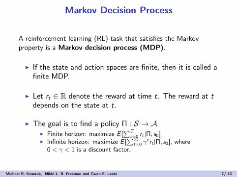
Markov Decision Process

A reinforcement learning (RL) task that satisfies the Markov

property is a Markov decision process (MDP).

I If the state and action spaces are finite, then it is called afinite MDP.

I Let rt ∈ R denote the reward at time t. The reward at tdepends on the state at t.

I The goal is to find a policy Π : S → AI Finite horizon: maximize E [

∑Tt=0 rt |Π, s0]

I Infinite horizon: maximize E [∑∞

t=0 γtrt |Π, s0], where

0 < γ < 1 is a discount factor.


MDPs in Precision Medicine

I MDPs are a way to frame precision medicine problems.

I The two methods we will consider in this lecture useMDPs to consider estimating dynamic treatment regimesin more general settings than we have seen so far.

I Ertefaie and Strawderman (2018) consider an indefinitetime period setting.

I Luckett et al. (2019+) consider the infinite time horizonwith a clinical application to mHealth and type 1 diabetes.


Outline





The indefinite time period setting

I So far we have considered a wide range of methods forestimating dynamic treatment regimes.

I Q-learning, OWL, etc.

I Each of these methods rely on backward induction toestimate the optimal DTR.

I These methods cannot extrapolate beyond the timehorizon in the observed data.

I For diseases such as cancer, this might be ok. For chronicdiseases, this limitation is a departure from reality. (Notethat some cancers are now being treated as chronicdiseases, too).

I Ertefaie and Strawderman (2018) propose a method forestimating optimal DTRs over an indefinite time horizon.


Notation

I St , t = 0, 1, . . . denotes a summary of a subject’s healthhistory through time t.

I St takes values in S? = S ∪ {c}, where S ∩ {c} = ∅.I c represents an absorbing state, such as death.

I For convenience, assume that S is finite.

I At is the treatment assigned at t after measuring St .

I Let A be a finite set containing m possible treatment actions.

I For t ≥ 0 and x ∈ S, suppose that At takes values in As

where As is a subset of A consisting of 0 < ms ≤ mtreatments and ∪s∈SAs = A.

I For any t such that St = c , let At ∈ Ac = {u}, where udenotes undefined.


Notation (cont.)

I Let H = (S0,A0, . . . , ST−1,AT−1, ST ) be the data on asubject observed from t = 0 until death,

T = inf{t ≥ 1 : St = c}.

I Let St and At denote the respective process histories upto and including time t.


Assumption 1: Time-homogeneous Markov behavior

Time-homogeneous Markov behavior assumption: Thedata-generating process satisfies

St+1 ⊥ {St−1, At−1}|St ,At

for t ≥ 1. In addition, for t ≥ 1, the transition probabilities satisfy

pr(St+1 = s ′|St = s,At = a) = pr(S1 = s ′|S0 = s,A0 = a)

= p(s ′|s, a) > 0

for s ′ ∈ S?, s ∈ S , a ∈ As ; moreover

pr(St+1 = c ,At+1 = u|St = c ,At = u) = 1.


Assumption 2: Positivity

Positivity assumpmtion: Let pAt |St ,At−1(a|s, a) be the probability

of receiving treatment a given St = s and At−1 = a. Then

pAt |St ,At−1(a|s, a) > 0

for each action a ∈ ASt and for each possible value of s and of a.


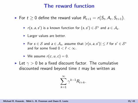
The reward function

I For t ≥ 0 define the reward value Rt+1 = r(St ,At , St+1).

I r(s, a, s ′) is a known function for (s, s ′) ∈ S? and a ∈ As .

I Larger values are better.

I For s ∈ S and a ∈ As , assume that |r(s, a, s ′)| ≤ r for s ′ ∈ S?and for some fixed 0 < r <∞.

I We assume r(c , u, c) = 0.

I Let γ > 0 be a fixed discount factor. The cumulativediscounted reward beyond time t may be written as

∞∑k=1

γk−1Rt+k .


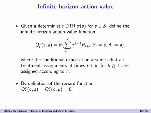
Infinite-horizon action-value

I Given a deterministic DTR π(s) for s ∈ S, define theinfinite-horizon action-value function

Qπt (s, a) = E (

∞∑k=1

γk−1Rt+k |St = s,At = a),

where the conditional expectation assumes that alltreatment assignments at times t + k , for k ≥ 1, areassigned according to π.

I By definition of the reward functionQπ

t (c , a) = Qπt (c , u) = 0.


Characterization of optimal DTR

I The optimal DTR is characterized as the regime that, ifimplemented, would lead to an optimal action-valuefunction for each pair (s, a) when s ∈ S.

I Under assumption 1, Qπt (s, a) does not depend on t and

is finite whenever γ < 1.

I For γ < 1, define the optimal action-value function asQ∗(s, a) = maxπ Q

πt (s, a), which can be shown to satisfy

Q∗(s, a) = E{Rt+1 + γ maxa′∈ASt+1

Q∗(St+1, a′)|St = s,At = a} (1)

for s ∈ S and a ∈ As .

I The optimal treatment regime: π∗(s) = argmaxa∈AsQ∗(s, a).


Estimating Q∗(s, a)

I To estimate the optimal DTR, we need to estimate theoptimal action-value function (1).

I A way forward is to model Q∗(s, a) as a linear function,say

Q∗(s, a) = Qθ0(s, a) = θᵀ0ϕ(s, a)

whereI Qθ(s, a) = θᵀϕ(s, a),I θ is a p-dimensional parameter, andI ϕ(s, a) a p-vector of features summarizing (s, a).

I To ensure that Qθ0(c , a) = 0, we require ϕ(c , a) = 0.


Estimating Q∗(s, a) (cont.)

I Under these assumptions, π∗(s) = argmaxa∈AsQθ0(s, a)

for s ∈ S.

I From here, estimating equations can be devised for

subjects who are followed from t = 0 to T and subjects

who are only followed until T = min(T , T ) where0 < T <∞ corresponds to the end of follow-up (maxnumber of possible decision points).


Estimating equationI First, we consider an estimating equation for θ0 for a

subject followed from time t = 0 to T .I Define

δt+1(θ) = Rt+1 − Qθ(St ,At) + γ maxa′∈ASt+1

Qθ(St+1, a′)

as the temporal difference error.I In view of (1), we have

E{δt+1(θ0)|St = s,At = a} = 0 (t ≥ 0).

I Hence, under our assumptions

E

{ T−1∑t=1

δt+1(θ0)ϕ(St ,At)

}= 0

where ϕ(s, a) = ∇θQθ(s, a).I This relationship suggests an estimating equation for θ0.


Estimating equation (cont.)

I With the intuition of the EE on the previous slide, now weconsider an estimating equation for a subject that can

only be followed until T = min(T , T ).

I Because T is fixed, we have D(θ0) = 0, where

D(θ) = E

{ T−1∑t=0

I (T > t)δt+1(θ)ϕ(St ,At)

}

= E

{ T−1∑t=0

δt+1(θ)ϕ(St ,At)

}.

where the second equality results from

I (T > t)δt+1(θ) = δt+1(θ) for t ≥ 0.


Estimating equation (cont.)

I Thus

D(θ) = Pn

{ T−1∑t=0

δt+1(θ)ϕ(St ,At)

}

= Pn

{ T−1∑t=0

δt+1(θ)ϕ(St ,At)

}(2)

is an unbiased estimating function for θ0, where theobserved data consists of the trajectoriesHi = (Si ,0,Ai ,0, . . . , Si ,Ti−1,Ai ,Ti−1, STi

).

I If D(θ) = 0 has a unique solution θ, then

Q∗(s, a) = Qθ(s, a) and the optimal DTR can beestimated by π∗(s) = argmaxa∈As

Qθ(s, a).


Estimation

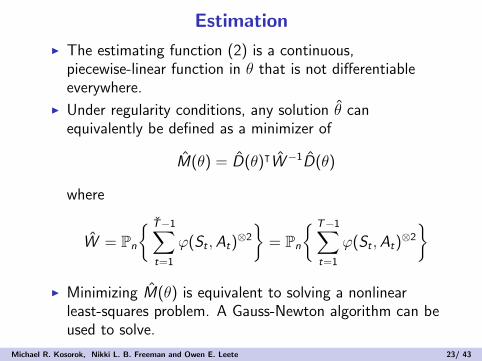
I The estimating function (2) is a continuous,piecewise-linear function in θ that is not differentiableeverywhere.

I Under regularity conditions, any solution θ canequivalently be defined as a minimizer of

M(θ) = D(θ)ᵀW−1D(θ)

where

W = Pn

{ T−1∑t=1

ϕ(St ,At)⊗2

}= Pn

{ T−1∑t=1

ϕ(St ,At)⊗2

}I Minimizing M(θ) is equivalent to solving a nonlinear

least-squares problem. A Gauss-Newton algorithm can beused to solve.


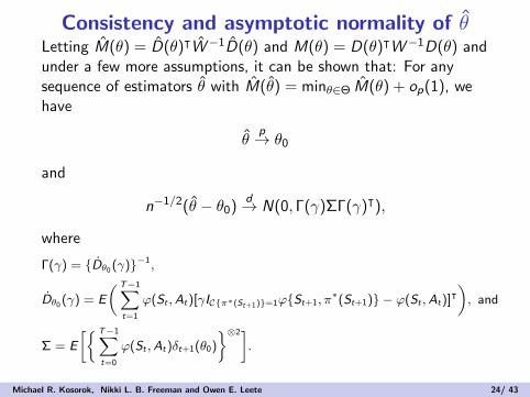
Consistency and asymptotic normality of θLetting M(θ) = D(θ)ᵀW−1D(θ) and M(θ) = D(θ)ᵀW−1D(θ) andunder a few more assumptions, it can be shown that: For anysequence of estimators θ with M(θ) = minθ∈Θ M(θ) + op(1), wehave

θp→ θ0

and

n−1/2(θ − θ0)d→ N(0, Γ(γ)ΣΓ(γ)ᵀ),

where

Γ(γ) = {Dθ0 (γ)}−1,

Dθ0 (γ) = E

( T−1∑t=1

ϕ(St ,At)[γIC{π∗(St+1)}=1ϕ{St+1, π∗(St+1)} − ϕ(St ,At)]ᵀ

), and

Σ = E

[{ T−1∑t=0

ϕ(St ,At)δt+1(θ0)

}⊗2].


Outline





Introduction

I Luckett et al. (2019+) develop estimation techniques(using data collected with mobile devices) for dynamictreatment regimes (which can be implemented asmHealth interventions)

I Motivating example: type 1 diabetes

I Understand type 1 diabetes (T1D) and how it is managed

I Develop tailored mHealth interventions for T1D management


What is T1D?

I Autoimmune disease wherein the pancreas producesinsufficient insulin

I Daily regimen of monitoring glucose and replacing insulin

I Hypo- and hyperglycemia result from poor management

I Glucose levels affected by insulin, diet, and physicalactivity

I Studied in an outpatient setting by Maahs et al. (2012)


A Day in the Life of a T1D Patient

time (half−hours)

glu

co

se

(m

g/d

L)

0 10 20 30 40 48

50

10

01

50

20

02

50

glucose

insulin

activity

food

Figure 1: Time course of glucose level and other quantities.


Mobile technology in T1D care

Mobile devices can be used to administer treatment and assist withdata collection in an outpatient setting, including

I Continuous glucose monitoring

I Accelerometers to track physical activity

I Insulin pumps to administer and log injections

These technologies can be incorporated using mobile phones.


Goals

Methodological goals:

I Estimate dynamic treatment regimes for use in mobilehealth

I Infinite time horizon, minimal modeling assumptions

I Observational data with minute-by-minute observations

I Online estimation to facilitate real-time decision making

Clinical goals:

I Provide patients information on the best actions tostabilize glucose

I Recommendations that are dynamic and personalized tothe patient


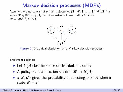
Markov decision processes (MDPs)Assume the data consist of n i.i.d. trajectories

(S1,A1,S2, . . . ,ST ,AT ,ST+1

)where St ∈ Rp, At ∈ A, and there exists a known utility functionU t = u(St+1,At ,St).

Figure 2: Graphical depiction of a Markov decision process.

Treatment regimes:

I Let B(A) be the space of distributions on AI A policy, π, is a function π : dom St → B(A)

I π(at ; st) gives the probability of selecting at ∈ A when instate St = st


The state-value function

I The state-value function is

V (π, st) = E

{∑k≥0

γkU∗(t+k)(π)∣∣St = st

}

for a discount factor γ ∈ (0, 1)

I For a distribution, R, define the value of π,VR(π) =

∫V (π, s)dR(s)

I For a class of regimes, Π, the optimal regime, πoptR ∈ Π,

satisfiesVR(πopt

R ) ≥ VR(π)

for all π ∈ Π.


An estimating equation for V (π, s)

Let µt(at ; st) = Pr(At = at |St = st) for each t ≥ 1.

LemmaAssume strong ignorability, consistency, and positivity. Let π denote anarbitrary regime and γ ∈ (0, 1) a discount factor. Then, providedinterchange of the sum and integration is justified, the state-valuefunction of π at st is

V (π, st) =∑k≥0

E

[γkU t+k

{k∏

v=0

π(Av+t ; Sv+t)

µv+t(Av+t ; Sv+t)

}∣∣∣∣St = st

].

This result will form the basis of an estimating equation forV (π, s).


An estimating equation for V (π, s) (continued)

It follows that

0 = E[π(At ; St)

µt(At ; St)

{Ut + γV (π,St+1)− V (π,St)

}ψ(St)

],

for any function ψ (an importance-weighted version of the Bellmanequation). An estimating equation for V (π, s) is

Λn(π, θπ) =1

n

n∑i=1

Ti∑t=1

π(Ati ; St

i )

µt(Ati ; St

i )

{Uti + γV (π,St+1

i ; θπ)− V (π,Sti ; θ

π)}∇θπV (π,St

i ; θπ),

where V (π,S; θπ) is a parametric model for the state-valuefunction.


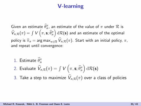
V-learning

Given an estimate θπn , an estimate of the value of π under R is

Vn,R(π) =∫V(π, s; θπn

)dR(s) and an estimate of the optimal

policy is πn = arg maxπ∈Π Vn,R(π). Start with an initial policy, π,and repeat until convergence:

1. Estimate θπn

2. Evaluate Vn,R(π) =∫V(π, s; θπn

)dR(s)

3. Take a step to maximize Vn,R(π) over a class of policies


Online estimation

Given n i.i.d. copies of accumulating data{(

S1,A1,S2, . . .)}n

i=1,

I Select actions using estimated policy and estimate a newpolicy

I Introduce randomness into deterministic policies (e.g.,ε-greedy)

The optimal policy at time t is based on the estimating equation

Λn,t(π, θπ) =

1

n

n∑i=1

t∑v=1

π(Avi ; Sv

i )

πv−1n (Av

i ; Svi )

×{Uvi + γV (π,Sv+1

i ; θπ)− V (π,Svi ; θπ)

}∇θπV (π,Sv

i ; θπ).

Note that πt−1n replaces µt as the data-generating policy.


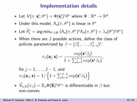
Implementation details

I Let V (π, sti ; θπ) = Φ(sti )

ᵀθπ where Φ : Rp → Rq

I Under this model, Λn(π, θπ) is linear in θπ

I Let θπn = arg minθπ∈Θ {Λn(π, θπ)ᵀΛn(π, θπ) + λn(θπ)ᵀθπ}I When there are J possible actions, define the class of

policies parametrized by β = (βᵀ1 , . . . , β

ᵀJ−1)ᵀ:

πβ(aj ; s) =exp(sᵀβj)

1 +∑J−1

k=1 exp(sᵀβk),

for j = 1, . . . , J − 1, and

πβ(aJ ; s) = 1/{

1 +∑J−1

k=1 exp(sᵀβk)}

I Vn,R(πβ) = EnΦ(S)ᵀθπβ is differentiable in β butnon-convex


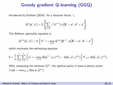
Greedy gradient Q-learning (GGQ)

Introduced by Ertefaie (2014): for a discount factor, γ,

Qπ(st , at) = E

∑k≥0

γkU t+k(π)∣∣∣St = st ,At = at

.

The Bellman optimality equation is

Qopt(st , at) = E{U t + γmax

a∈AQopt(St+1, a)

∣∣∣St = st ,At = at}.

which motivates the estimating equation

0 =1

n

n∑i=1

Ti∑t=1

{uti + γmax

a∈AQ(st+1

i , a; ηopt)− Q(sti , ati ; η

opt)

}∇ηoptQ(sti , a

ti ; η

opt).

After computing the estimate ηoptn , the optimal policy in state s selects action

πn(s) = maxa∈AQ(s, a; ηoptn ).


Asymptotic Inference for V-Learning

I We obtain uniform asymptotic normality for keyparameters and predictions

I Main technical tools:I Donsker theorem for β-mixing stationary processes based on

bracketing entropy (Dedecker and Louhichi, 2002)I New bracketing entropy preservation results for products of

function classes

I Issue: Need Donsker theorems for non-stationaryprocesses for certain types of online V-learning


T1D outpatient data set

I Maahs et al. (2012) followed N = 31 patients for a totalof 5 days

I Insulin injections were logged via an insulin pump

I Glucose levels were tracked using continuous glucosemonitoring

I Dietary intake data were reported in phone interviews

I Utility is the weighted sum of glycemic status

I We want to estimate a treatment policy to control glucosethrough a personalized insulin regimen or personalizedrecommendations for insulin, diet, and exercise

I Evaluate with parametric value estimate,

Vn,R(πn) = EnΦ(S)ᵀθπnn


An application to T1D data

Action space Basis γ = 0.7 γ = 0.8 γ = 0.9Binary Linear −6.20 −9.35 −15.99

Polynomial −3.91 −9.03 −17.50Gaussian −3.44 −13.09 −25.52

Multiple Linear −6.47 −9.92 −0.49Polynomial −2.44 −6.80 −14.48Gaussian −8.45 −3.58 −21.18

Observational policy −6.77 −11.28 −21.79

Table 1: Parametric value estimates for V-learning applied to type 1diabetes data.


Example hyperglycemic (229 mg/dL) patient

Action ProbabilityNo action < 0.0001Physical activity < 0.0001Food intake < 0.0001Food and activity < 0.0001Insulin 0.7856Insulin and activity 0.2143Insulin and food 0.0002Insulin, food, and activity < 0.0001

Table 2: Probabilities for each action as recommended by estimatedpolicy for one example hyperglycemic patient.


Conclusions

I Glucose is known to depend on insulin, diet, and exercise

I Optimal treatment regimes for T1D depend on lifestyleconsiderations; little work has been done to constructdecision rules for T1D management in a statisticallyrigorous way

I Advantages of V-learning include

I Flexibility in models for V (π, s; θπ) and πβ(a; s)

I Minimal assumptions about the data-generating process

I Randomized decision rules for online estimation

I No need to model a non-smooth functional of the data

I A tailored treatment regime delivered through mobiledevices may help to reduce hypo- and hyperglycemia inT1D patients


Precision Medicine: Lecture 11 Markov Decision Processes

Documents

Transcript of Precision Medicine: Lecture 11 Markov Decision Processes