Precise ellipse estimation without contour point...

Machine Vision and Applications manuscript No.(will be inserted by the editor)

Jean-Nicolas Ouellet · Patrick Hebert

Precise ellipse estimation without contour point extraction

Received: date / Accepted: date

Abstract This paper presents a simple linear operator that accurately estimates the parameters of ellipse

features. Based on the dual conic model, the operator directly exploits the raw gradient information in the

neighborhood of an ellipse’s boundary, thus avoiding the intermediate stage of precisely extracting individual

edge points. Moreover, under the dual representation, the dual conic can easily be constrained to a dual

ellipse when minimizing the algebraic distance. The new operator is compared to other estimation approaches,

including those limited to the center position, in simulation as well as in real situation experiments.

Keywords ellipse targets · conic · dual conic · dual ellipse · geometric fitting · Forstner operator

Jean-Nicolas Ouellet

Laval University

Canada (Qc), Quebec

G1K 7P4

Tel.: +1-418-656-2131-4786

Fax: +1-418-656-3594

E-mail: [email protected]

Patrick Hebert

Laval University

Canada (Qc), Quebec

G1K 7P4

Tel.: +1-418-656-2131-4479

Fax: +1-418-656-3594

E-mail: [email protected]

2 Jean-Nicolas Ouellet, Patrick Hebert

1 Introduction

Precise estimation of an ellipse in an image usually consists in accurately extracting contour points with

subpixel precision before fitting ellipse parameters on the obtained set of points. Until recently, numerous

methods have been proposed for fitting an ellipse from a given set of contour points [2–4, 6, 12, 13, 16]. They

differ from each other depending on their precision, accuracy, robustness to outliers or on their ability to fit

parameters on partial ellipse contours. All these methods rely on a set of contour points that are extracted

beforehand. Nevertheless, extracting contour points usually subsumes multiple stages including gradient es-

timation, non-maximum suppression, thresholding, and subpixel estimation.

Extracting contour points imposes making a decision for each of those points based on neighboring pixels

in the image. The following question thus arises. Is it possible to develop a more direct method that precludes

the extraction of a set of contour points? One would directly exploit the information encoded in all pixels

in the ellipse neighborhood. By eliminating precise contour point extraction, the method would be greatly

simplified and the uncertainty on the recovered ellipse parameters will be assessed more closely to the image

data. Another motivation for developing such an approach is the possibility to process low contrast images

where each contour point can hardly be extracted along the ellipse.

Formally, given a set of pixels nearby an complete ellipse contour in a real image, what are the ellipse

parameters? Although the limitation to complete ellipses might appear restrictive, it is of great interest for

camera calibration and precise measurement applications where it is common to use physical circular targets

that project into ellipses in an image [10]. In these applications, partial ellipses lead to a less reliable estimation

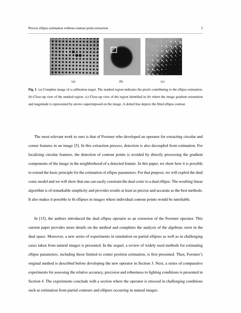
and are generally avoided. In Fig. 1(a), a rectangular area enclosing an ellipse is shown. We develop a method

that can accurately fit the ellipse’s parameters from all the pixels that lie inside such an area or preferably

nearby the ellipse’s contour. More precisely, we will show how one can estimate the ellipse’s parameters

directly from the gradient vector field. Fig. 1(c) is a close up view where the gradient vector field as well

as the fitted ellipse contour are superimposed on the image. It is important to note that we focus on ellipse

parameter estimation, as opposed to ellipse detection. Although their detection is simple from calibration

targets, in more general situations it is assumed that the set of pixels describing an ellipse can be roughly

identified beforehand.

Precise ellipse estimation without contour point extraction 3

(a) (b) (c)

Fig. 1 (a) Complete image of a calibration target. The marked region indicates the pixels contributing to the ellipse estimation.

(b) Close-up view of the marked region. (c) Close-up view of the region identified in (b) where the image gradient orientation

and magnitude is represented by arrows superimposed on the image. A dotted line depicts the fitted ellipse contour.

The most relevant work to ours is that of Forstner who developed an operator for extracting circular and

corner features in an image [5]. In this extraction process, detection is also decoupled from estimation. For

localizing circular features, the detection of contour points is avoided by directly processing the gradient

components of the image in the neighborhood of a detected feature. In this paper, we show how it is possible

to extend the basic principle for the estimation of ellipse parameters. For that purpose, we will exploit the dual

conic model and we will show that one can easily constrain the dual conic to a dual ellipse. The resulting linear

algorithm is of remarkable simplicity and provides results at least as precise and accurate as the best methods.

It also makes it possible to fit ellipses in images where individual contour points would be unreliable.

In [15], the authors introduced the dual ellipse operator as an extension of the Forstner operator. This

current paper provides more details on the method and completes the analysis of the algebraic error in the

dual space. Moreover, a new series of experiments in simulation on partial ellipses as well as in challenging

cases taken from natural images is presented. In the sequel, a review of widely used methods for estimating

ellipse parameters, including those limited to center position estimation, is first presented. Then, Forstner’s

original method is described before developing the new operator in Section 3. Next, a series of comparative

experiments for assessing the relative accuracy, precision and robustness to lighting conditions is presented in

Section 4. The experiments conclude with a section where the operator is stressed in challenging conditions

such as estimation from partial contours and ellipses occurring in natural images.


2 Related work

An ellipse can be estimated from the image intensity or its gradient. Intensity-based methods are also referred

to as direct methods [18] when they directly exploit the image intensity with no transformation or derivation.

One simple method which returns the coordinates of the feature is the gray-scale centroid, where for a given

region, the intensity of each pixel is used to weigh its contribution to the estimation of the intensity center

of mass. Integrating over all pixels in the region provides good immunity to noise. However, intensity-based

methods like centroid estimation are particularly sensitive to non-uniform illumination. The causes of non-

uniform illumination are frequent and various, e.g. light sources, vignetting or reflections on specular surfaces.

Gradient-based methods are less affected by non-uniform illumination. Nevertheless, the derivation process

involved makes them more sensitive to noise. Generally, these latter methods are composed of two dis-

tinct steps; the edges of a region are first identified after non-maxima suppression and a conic is fitted

to the edge points. The simplest method, linear least-square, minimizes the algebraic error associated with

the points. Since the linear system is homogeneous, a constraint must be imposed on the conic parameters

Θ = [A, B, C, D, E, F]T to avoid the trivial solution Θ = 0. Many possible constraints were studied in order

to estimate the best conic from a set of points, e.g. F = 1, ‖Θ‖ = 1 (see [4, 16] for a review). Nevertheless, it

is essential for a conic estimator to be invariant to Euclidean transformations (translation, rotation, scale) [1].

According to this definition the constraints ‖Θ‖ = 1 and F = 1 are not invariant. On the other hand, the

expression 4AC −B2 is a conic invariant and can be formulated as the quadratic constraint 4AC −B2 = 1.

Under this constraint, the parameters minimizing the algebraic error, which are obtained via a generalized

eigensystem, describe elliptical shapes [3]. However, in the presence of partial ellipses, this method, and all

other methods based on the algebraic error, will underestimate the eccentricity of the ellipse [20]. Different

iterative algorithms were introduced to reduce or compensate for the bias [2, 12]. Still, given that ellipses are

complete, the effect of the bias is practically nonexistent and there are no significant differences among high

quality fitting methods [4]. In this situation, it is advantageous to employ the simplest method.

Estimating a conic from pixels’ centers identified as local maxima is generally inaccurate. A better esti-

mation is obtained from the edge points whose positions are known with subpixel precision. A simple way

to achieve subpixel precision is to perform a parabolic interpolation of the gradient maximum along the edge

direction. The method is simple but the interpolation is sensitive to noise. An alternative is proposed in [19]


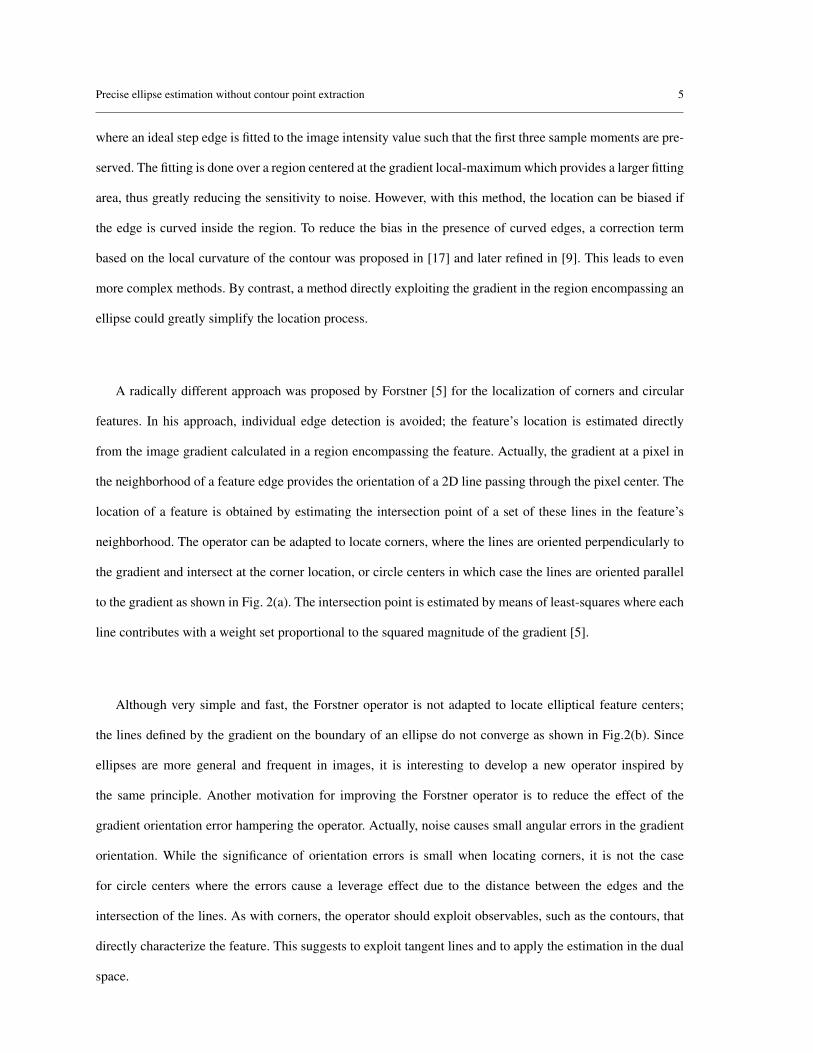
where an ideal step edge is fitted to the image intensity value such that the first three sample moments are pre-

served. The fitting is done over a region centered at the gradient local-maximum which provides a larger fitting

area, thus greatly reducing the sensitivity to noise. However, with this method, the location can be biased if

the edge is curved inside the region. To reduce the bias in the presence of curved edges, a correction term

based on the local curvature of the contour was proposed in [17] and later refined in [9]. This leads to even

more complex methods. By contrast, a method directly exploiting the gradient in the region encompassing an

ellipse could greatly simplify the location process.

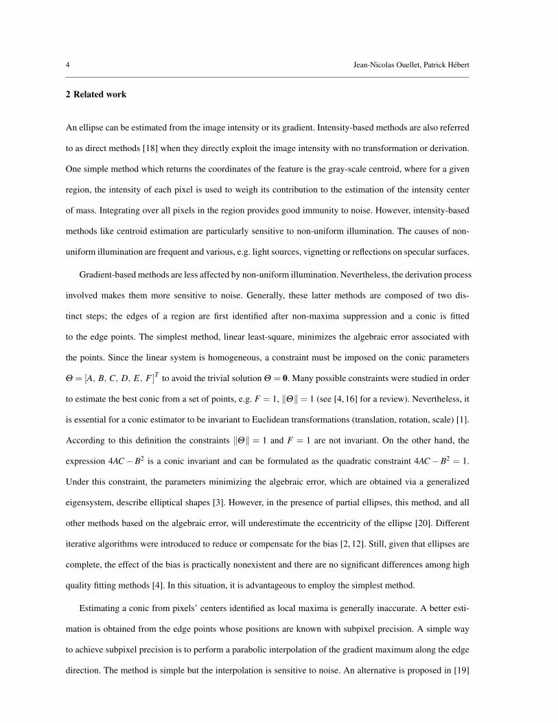
A radically different approach was proposed by Forstner [5] for the localization of corners and circular

features. In his approach, individual edge detection is avoided; the feature’s location is estimated directly

from the image gradient calculated in a region encompassing the feature. Actually, the gradient at a pixel in

the neighborhood of a feature edge provides the orientation of a 2D line passing through the pixel center. The

location of a feature is obtained by estimating the intersection point of a set of these lines in the feature’s

neighborhood. The operator can be adapted to locate corners, where the lines are oriented perpendicularly to

the gradient and intersect at the corner location, or circle centers in which case the lines are oriented parallel

to the gradient as shown in Fig. 2(a). The intersection point is estimated by means of least-squares where each

line contributes with a weight set proportional to the squared magnitude of the gradient [5].

Although very simple and fast, the Forstner operator is not adapted to locate elliptical feature centers;

the lines defined by the gradient on the boundary of an ellipse do not converge as shown in Fig.2(b). Since

ellipses are more general and frequent in images, it is interesting to develop a new operator inspired by

the same principle. Another motivation for improving the Forstner operator is to reduce the effect of the

gradient orientation error hampering the operator. Actually, noise causes small angular errors in the gradient

orientation. While the significance of orientation errors is small when locating corners, it is not the case

for circle centers where the errors cause a leverage effect due to the distance between the edges and the

intersection of the lines. As with corners, the operator should exploit observables, such as the contours, that

directly characterize the feature. This suggests to exploit tangent lines and to apply the estimation in the dual

space.


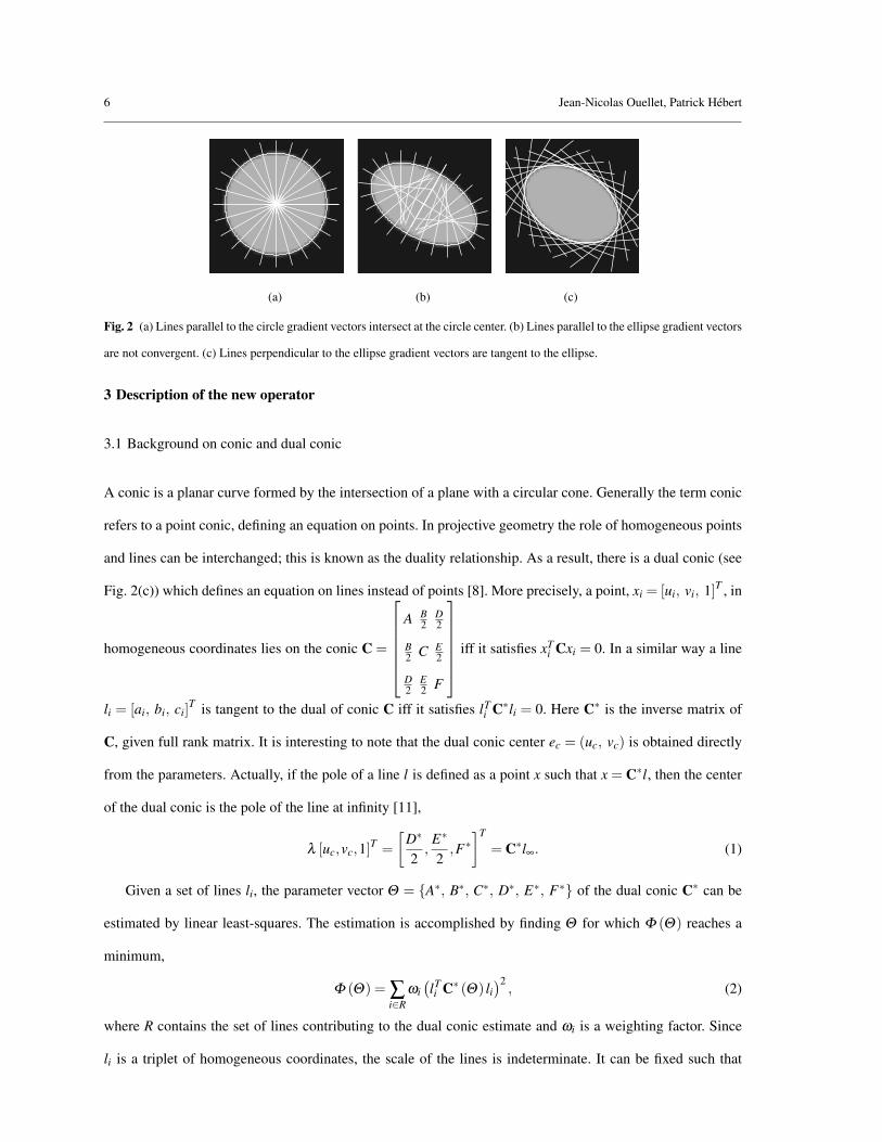
(a) (b) (c)

Fig. 2 (a) Lines parallel to the circle gradient vectors intersect at the circle center. (b) Lines parallel to the ellipse gradient vectors

are not convergent. (c) Lines perpendicular to the ellipse gradient vectors are tangent to the ellipse.

3 Description of the new operator

3.1 Background on conic and dual conic

A conic is a planar curve formed by the intersection of a plane with a circular cone. Generally the term conic

refers to a point conic, defining an equation on points. In projective geometry the role of homogeneous points

and lines can be interchanged; this is known as the duality relationship. As a result, there is a dual conic (see

Fig. 2(c)) which defines an equation on lines instead of points [8]. More precisely, a point, xi = [ui, vi, 1]T , in

homogeneous coordinates lies on the conic C =

A B2

D2

B2

C E2

D2

E2

F

iff it satisfies xTi Cxi = 0. In a similar way a line

li = [ai, bi, ci]T

is tangent to the dual of conic C iff it satisfies lTi C∗li = 0. Here C∗ is the inverse matrix of

C, given full rank matrix. It is interesting to note that the dual conic center ec = (uc, vc) is obtained directly

from the parameters. Actually, if the pole of a line l is defined as a point x such that x = C∗l, then the center

of the dual conic is the pole of the line at infinity [11],

λ [uc,vc,1]T =

[

D∗

2,

E∗

2,F∗

]T

= C∗l∞. (1)

Given a set of lines li, the parameter vector Θ = {A∗, B∗, C∗, D∗, E∗, F∗} of the dual conic C∗ can be

estimated by linear least-squares. The estimation is accomplished by finding Θ for which Φ (Θ) reaches a

minimum,

Φ (Θ) = ∑i∈R

ωi

(

lTi C∗ (Θ) li

)2, (2)

where R contains the set of lines contributing to the dual conic estimate and ωi is a weighting factor. Since

li is a triplet of homogeneous coordinates, the scale of the lines is indeterminate. It can be fixed such that


‖a,b‖ = 1. Normal equations derived from Eq. (2) are linear in Θ and lead to the following form:

[

∑i∈R

ω2i KiK

Ti

]

[Θ ] = 0, (3)

where Ki is composed of line coefficients such that Ki =[

a2i , aibi, b2

i , aici, bici, c2i

]T. This system can be

solved under the constraint ‖Θ‖ = 1 using the singular value decomposition (SVD). However, this constraint

is not invariant to Euclidean transformations [1]. A more appropriate constraint is introduced in the next

section.

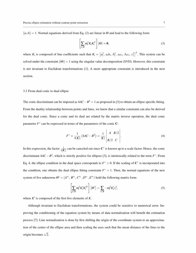
3.2 From dual conic to dual ellipse

The conic discriminant can be imposed as 4AC−B2 = 1 as proposed in [3] to obtain an ellipse specific fitting.

From the duality relationship between points and lines, we know that a similar constraint can also be derived

for the dual conic. Since a conic and its dual are related by the matrix inverse operation, the dual conic

parameter F∗ can be expressed in terms of the parameters of the conic C:

F∗ =1

4 |C|(

4AC−B2)

=1

|C|

∣

∣

∣

∣

∣

∣

∣

A B/2

B/2 C

∣

∣

∣

∣

∣

∣

∣

. (4)

In this expression, the factor 1

4|C| can be canceled out since C∗ is known up to a scale factor. Hence, the conic

discriminant 4AC−B2, which is strictly positive for ellipses [3], is intrinsically related to the term F∗. From

Eq. 4, the ellipse condition in the dual space corresponds to F∗ > 0. If the scaling of C∗ is incorporated into

the condition, one obtains the dual ellipse fitting constraint F∗ = 1. Then, the normal equations of the new

system of five unknowns Θ ′ = (A′∗, B′∗, C′∗ ,D′∗ ,E ′∗) hold the following matrix form:

[

∑i∈R

ω2i K′

i K′Ti

]

[

Θ ′] = ∑i∈R

−ω2i K′

i c2i , (5)

where K′ is composed of the first five elements of K.

Although invariant to Euclidean transformations, the system could be sensitive to numerical error. Im-

proving the conditioning of the equation system by means of data normalization will benefit the estimation

process [7]. Line normalization is done by first shifting the origin of the coordinate system to an approxima-

tion of the center of the ellipse area and then scaling the axes such that the mean distance of the lines to the

origin becomes√

2.


3.3 Dual ellipse estimation from images

The image gradient near a contour naturally provides the orientation of the contour normal. Therefore, given

a set of pixels belonging to the neighborhood of an ellipse, a set of lines can be constructed from the gradient

to solve for Eq. (5). More precisely, when the image gradient ∇Ii = [Iui, Ivi]T

at a pixel xi is not null, it defines

the normal orientation of a line passing through the pixel center such that:

li =[

Iui, Ivi, −∇ITi xi

]T. (6)

From this definition, each line contributes with a weight equal to the squared gradient magnitude in Eq. (5).

There are two advantages to give higher importance to observations where the gradient magnitude is strong.

First, the operator will focus on the active zone of the gradient where the ellipse contour has high probability

of being located. Thus, a precise interpolation step is not required, the operator processes all pixels. Second,

the robustness to noise is improved, particularly in regions of weak gradient where the line orientation is not

well defined.

The resulting operator requires very few steps and computations. Actually, each pixel of the region con-

tributes to the sums in Eq. 5. Once the parameters are obtained, one can further estimate the variance-

covariance matrix of the dual ellipse parameters which is particularly meaningful. The 2x2 submatrix in-

cluding D∗, E∗ and their covariance term, directly provides the uncertainty of the center coordinates. The

development of the covariance expression is detailed in [15].

3.4 Algebraic error in the dual space

Dual conic and point conic share a strong relationship in the representation of the algebraic error. The relation-

ship comes from the equivalence of the error expressions under a conic matrix inversion. In the dual space,

the error is proportional to the distance between a tangent li and its pole xi = C∗li whereas, in the normal

space, the error is proportional to the distance between a point xi and its polar li = Cxi. The dual conic error

is represented as εi in Fig.3(a). Also, for both the conic and dual conic, the algebraic error evolves differently

as the Euclidean distance increases along the ellipse contour. This can be observed from the spacing between

isocontours in Fig.3(b) and Fig.3(c), which is different for regions of low and high curvature. In the figure, the


∇Ii

ǫi

xi = C∗

li

li

C∗

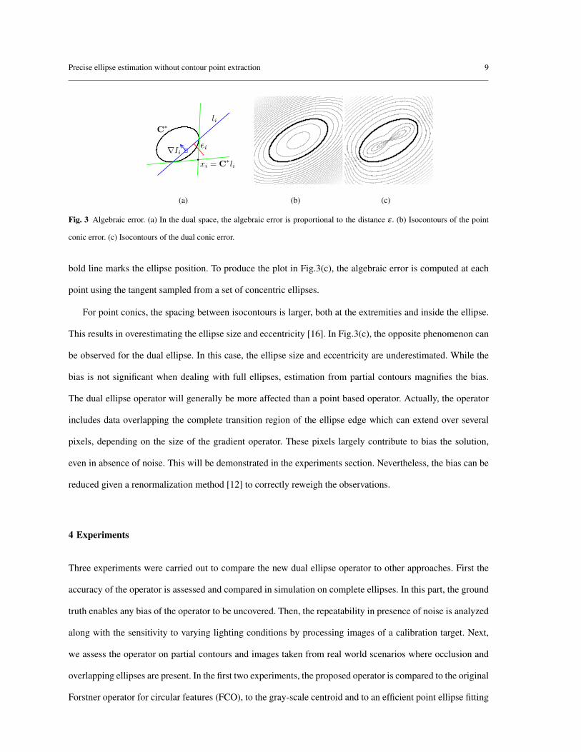
(a) (b) (c)

Fig. 3 Algebraic error. (a) In the dual space, the algebraic error is proportional to the distance ε . (b) Isocontours of the point

conic error. (c) Isocontours of the dual conic error.

bold line marks the ellipse position. To produce the plot in Fig.3(c), the algebraic error is computed at each

point using the tangent sampled from a set of concentric ellipses.

For point conics, the spacing between isocontours is larger, both at the extremities and inside the ellipse.

This results in overestimating the ellipse size and eccentricity [16]. In Fig.3(c), the opposite phenomenon can

be observed for the dual ellipse. In this case, the ellipse size and eccentricity are underestimated. While the

bias is not significant when dealing with full ellipses, estimation from partial contours magnifies the bias.

The dual ellipse operator will generally be more affected than a point based operator. Actually, the operator

includes data overlapping the complete transition region of the ellipse edge which can extend over several

pixels, depending on the size of the gradient operator. These pixels largely contribute to bias the solution,

even in absence of noise. This will be demonstrated in the experiments section. Nevertheless, the bias can be

reduced given a renormalization method [12] to correctly reweigh the observations.

4 Experiments

Three experiments were carried out to compare the new dual ellipse operator to other approaches. First the

accuracy of the operator is assessed and compared in simulation on complete ellipses. In this part, the ground

truth enables any bias of the operator to be uncovered. Then, the repeatability in presence of noise is analyzed

along with the sensitivity to varying lighting conditions by processing images of a calibration target. Next,

we assess the operator on partial contours and images taken from real world scenarios where occlusion and

overlapping ellipses are present. In the first two experiments, the proposed operator is compared to the original

Forstner operator for circular features (FCO), to the gray-scale centroid and to an efficient point ellipse fitting


(a) (b) (c)

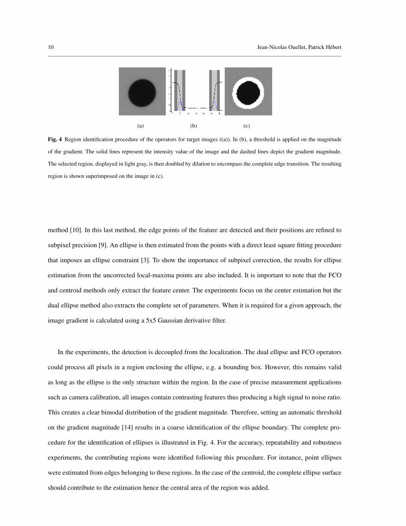
Fig. 4 Region identification procedure of the operators for target images ((a)). In (b), a threshold is applied on the magnitude

of the gradient. The solid lines represent the intensity value of the image and the dashed lines depict the gradient magnitude.

The selected region, displayed in light gray, is then doubled by dilation to encompass the complete edge transition. The resulting

region is shown superimposed on the image in (c).

method [10]. In this last method, the edge points of the feature are detected and their positions are refined to

subpixel precision [9]. An ellipse is then estimated from the points with a direct least square fitting procedure

that imposes an ellipse constraint [3]. To show the importance of subpixel correction, the results for ellipse

estimation from the uncorrected local-maxima points are also included. It is important to note that the FCO

and centroid methods only extract the feature center. The experiments focus on the center estimation but the

dual ellipse method also extracts the complete set of parameters. When it is required for a given approach, the

image gradient is calculated using a 5x5 Gaussian derivative filter.

In the experiments, the detection is decoupled from the localization. The dual ellipse and FCO operators

could process all pixels in a region enclosing the ellipse, e.g. a bounding box. However, this remains valid

as long as the ellipse is the only structure within the region. In the case of precise measurement applications

such as camera calibration, all images contain contrasting features thus producing a high signal to noise ratio.

This creates a clear bimodal distribution of the gradient magnitude. Therefore, setting an automatic threshold

on the gradient magnitude [14] results in a coarse identification of the ellipse boundary. The complete pro-

cedure for the identification of ellipses is illustrated in Fig. 4. For the accuracy, repeatability and robustness

experiments, the contributing regions were identified following this procedure. For instance, point ellipses

were estimated from edges belonging to these regions. In the case of the centroid, the complete ellipse surface

should contribute to the estimation hence the central area of the region was added.


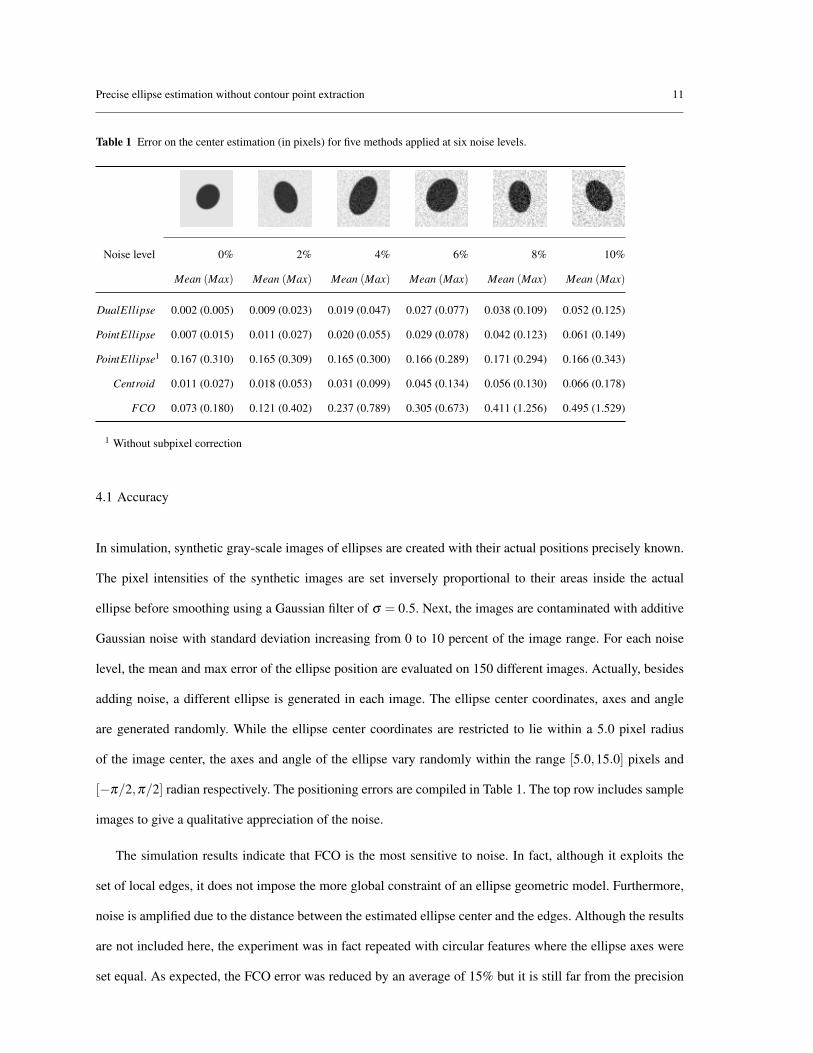
Table 1 Error on the center estimation (in pixels) for five methods applied at six noise levels.

Noise level 0% 2% 4% 6% 8% 10%

Mean (Max) Mean (Max) Mean (Max) Mean (Max) Mean (Max) Mean (Max)

DualEllipse 0.002 (0.005) 0.009 (0.023) 0.019 (0.047) 0.027 (0.077) 0.038 (0.109) 0.052 (0.125)

PointEllipse 0.007 (0.015) 0.011 (0.027) 0.020 (0.055) 0.029 (0.078) 0.042 (0.123) 0.061 (0.149)

PointEllipse1 0.167 (0.310) 0.165 (0.309) 0.165 (0.300) 0.166 (0.289) 0.171 (0.294) 0.166 (0.343)

Centroid 0.011 (0.027) 0.018 (0.053) 0.031 (0.099) 0.045 (0.134) 0.056 (0.130) 0.066 (0.178)

FCO 0.073 (0.180) 0.121 (0.402) 0.237 (0.789) 0.305 (0.673) 0.411 (1.256) 0.495 (1.529)

1 Without subpixel correction

4.1 Accuracy

In simulation, synthetic gray-scale images of ellipses are created with their actual positions precisely known.

The pixel intensities of the synthetic images are set inversely proportional to their areas inside the actual

ellipse before smoothing using a Gaussian filter of σ = 0.5. Next, the images are contaminated with additive

Gaussian noise with standard deviation increasing from 0 to 10 percent of the image range. For each noise

level, the mean and max error of the ellipse position are evaluated on 150 different images. Actually, besides

adding noise, a different ellipse is generated in each image. The ellipse center coordinates, axes and angle

are generated randomly. While the ellipse center coordinates are restricted to lie within a 5.0 pixel radius

of the image center, the axes and angle of the ellipse vary randomly within the range [5.0,15.0] pixels and

[−π/2,π/2] radian respectively. The positioning errors are compiled in Table 1. The top row includes sample

images to give a qualitative appreciation of the noise.

The simulation results indicate that FCO is the most sensitive to noise. In fact, although it exploits the

set of local edges, it does not impose the more global constraint of an ellipse geometric model. Furthermore,

noise is amplified due to the distance between the estimated ellipse center and the edges. Although the results

are not included here, the experiment was in fact repeated with circular features where the ellipse axes were

set equal. As expected, the FCO error was reduced by an average of 15% but it is still far from the precision


of the best methods. Since the gray-scale centroid method averages over all pixels of the feature, it shows

high immunity to noise, but it preserves a higher error. The dual ellipse operator is the most accurate in

all conditions. However, as noise increases, the estimation of the gradient orientation becomes less precise

and the dual ellipse and subpixel point ellipse methods present similar accuracy with a small, but systematic

advantage for the dual ellipse method. The high error obtained from ellipse fitting on raw points is due to

a random leap of position of the local maxima caused by image noise. This confirms the importance of an

accurate subpixel correction step before an ellipse can be estimated. Finally, the distribution of the error

vectors confirmed the absence of bias for all of the operators.

4.2 Repeatability and robustness to non-uniform illumination

The second part of the experiments aims to assess the repeatability of the operator and its robustness to

lighting variations in real conditions. In this experiment, the positions of the ellipses are unknown so we can

only compare the variation of position of the detected centers when varying illumination. For that purpose,

two sequences of 150 images of a planar calibration target comprising a set of circles are acquired (see Fig.

5). The camera and calibration target are set fixed to an optical table mounted on pneumatic vibration isolators

so both are perfectly still. The images were captured with a firewire camera at a resolution of 640x480 pixels.

Each image contains 130 low eccentricity ellipses with mean diameter of approximately 30 pixels. In order to

measure repeatability, we computed the mean and maximum ellipse displacements in the first sequence. Both

are listed in the first row of Table 2.

The second image sequence is acquired under different lighting conditions. To accomplish this, a new

light source is added to the scene before capturing the sequence. The addition of a new light creates a visible

change of illumination and prevents any setup manipulation between the two acquisitions. The effect of the

added light source can be observed in Fig. 5(b). Special care was taken to use high frequency fluorescent

lamps (300hz) having the same color spectrum to avoid any feature displacement due to chromatic aberration

or flickering. The displacement is taken as the distance between the mean center of a given ellipse in the first

sequence to its mean center in the second sequence. The mean and maximum displacements of the ellipses

between the two sequences are listed in the bottom row of Table 2.


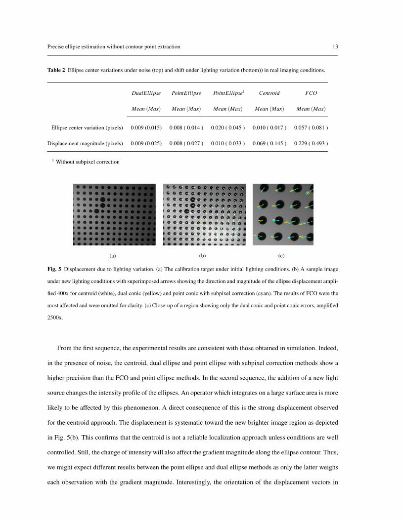
Table 2 Ellipse center variations under noise (top) and shift under lighting variation (bottom)) in real imaging conditions.

DualEllipse PointEllipse PointEllipse1 Centroid FCO

Mean (Max) Mean (Max) Mean (Max) Mean (Max) Mean (Max)

Ellipse center variation (pixels) 0.009 (0.015) 0.008 ( 0.014 ) 0.020 ( 0.045 ) 0.010 ( 0.017 ) 0.057 ( 0.081 )

Displacement magnitude (pixels) 0.009 (0.025) 0.008 ( 0.027 ) 0.010 ( 0.033 ) 0.069 ( 0.145 ) 0.229 ( 0.493 )

1 Without subpixel correction

(a) (b) (c)

Fig. 5 Displacement due to lighting variation. (a) The calibration target under initial lighting conditions. (b) A sample image

under new lighting conditions with superimposed arrows showing the direction and magnitude of the ellipse displacement ampli-

fied 400x for centroid (white), dual conic (yellow) and point conic with subpixel correction (cyan). The results of FCO were the

most affected and were omitted for clarity. (c) Close-up of a region showing only the dual conic and point conic errors, amplified

2500x.

From the first sequence, the experimental results are consistent with those obtained in simulation. Indeed,

in the presence of noise, the centroid, dual ellipse and point ellipse with subpixel correction methods show a

higher precision than the FCO and point ellipse methods. In the second sequence, the addition of a new light

source changes the intensity profile of the ellipses. An operator which integrates on a large surface area is more

likely to be affected by this phenomenon. A direct consequence of this is the strong displacement observed

for the centroid approach. The displacement is systematic toward the new brighter image region as depicted

in Fig. 5(b). This confirms that the centroid is not a reliable localization approach unless conditions are well

controlled. Still, the change of intensity will also affect the gradient magnitude along the ellipse contour. Thus,

we might expect different results between the point ellipse and dual ellipse methods as only the latter weighs

each observation with the gradient magnitude. Interestingly, the orientation of the displacement vectors in


(a) (b) (c) (d) (e) (f)

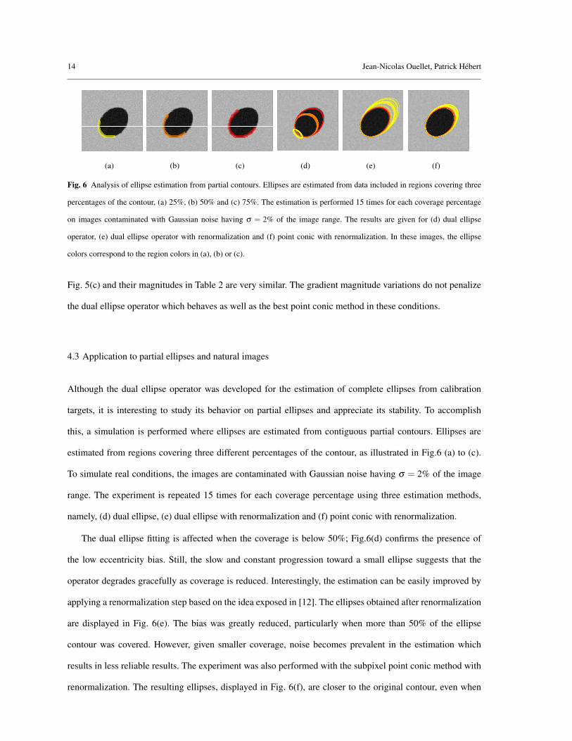
Fig. 6 Analysis of ellipse estimation from partial contours. Ellipses are estimated from data included in regions covering three

percentages of the contour, (a) 25%, (b) 50% and (c) 75%. The estimation is performed 15 times for each coverage percentage

on images contaminated with Gaussian noise having σ = 2% of the image range. The results are given for (d) dual ellipse

operator, (e) dual ellipse operator with renormalization and (f) point conic with renormalization. In these images, the ellipse

colors correspond to the region colors in (a), (b) or (c).

Fig. 5(c) and their magnitudes in Table 2 are very similar. The gradient magnitude variations do not penalize

the dual ellipse operator which behaves as well as the best point conic method in these conditions.

4.3 Application to partial ellipses and natural images

Although the dual ellipse operator was developed for the estimation of complete ellipses from calibration

targets, it is interesting to study its behavior on partial ellipses and appreciate its stability. To accomplish

this, a simulation is performed where ellipses are estimated from contiguous partial contours. Ellipses are

estimated from regions covering three different percentages of the contour, as illustrated in Fig.6 (a) to (c).

To simulate real conditions, the images are contaminated with Gaussian noise having σ = 2% of the image

range. The experiment is repeated 15 times for each coverage percentage using three estimation methods,

namely, (d) dual ellipse, (e) dual ellipse with renormalization and (f) point conic with renormalization.

The dual ellipse fitting is affected when the coverage is below 50%; Fig.6(d) confirms the presence of

the low eccentricity bias. Still, the slow and constant progression toward a small ellipse suggests that the

operator degrades gracefully as coverage is reduced. Interestingly, the estimation can be easily improved by

applying a renormalization step based on the idea exposed in [12]. The ellipses obtained after renormalization

are displayed in Fig. 6(e). The bias was greatly reduced, particularly when more than 50% of the ellipse

contour was covered. However, given smaller coverage, noise becomes prevalent in the estimation which

results in less reliable results. The experiment was also performed with the subpixel point conic method with

renormalization. The resulting ellipses, displayed in Fig. 6(f), are closer to the original contour, even when


(a) (b) (c) (d)

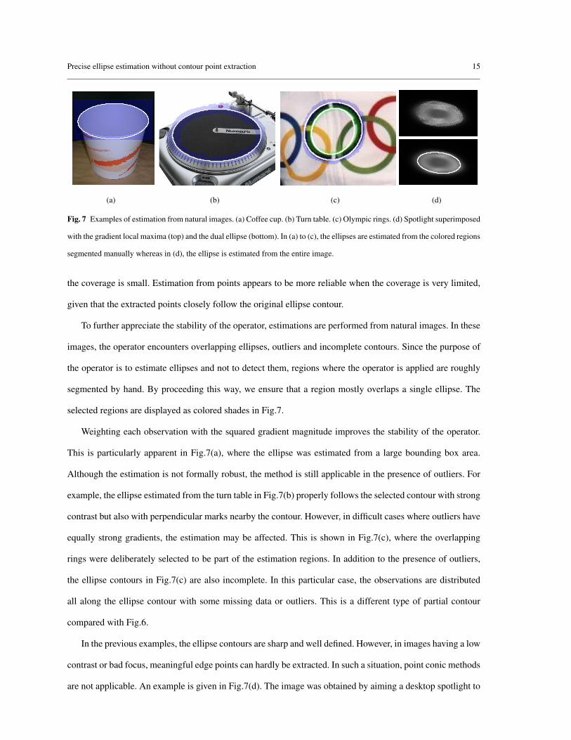
Fig. 7 Examples of estimation from natural images. (a) Coffee cup. (b) Turn table. (c) Olympic rings. (d) Spotlight superimposed

with the gradient local maxima (top) and the dual ellipse (bottom). In (a) to (c), the ellipses are estimated from the colored regions

segmented manually whereas in (d), the ellipse is estimated from the entire image.

the coverage is small. Estimation from points appears to be more reliable when the coverage is very limited,

given that the extracted points closely follow the original ellipse contour.

To further appreciate the stability of the operator, estimations are performed from natural images. In these

images, the operator encounters overlapping ellipses, outliers and incomplete contours. Since the purpose of

the operator is to estimate ellipses and not to detect them, regions where the operator is applied are roughly

segmented by hand. By proceeding this way, we ensure that a region mostly overlaps a single ellipse. The

selected regions are displayed as colored shades in Fig.7.

Weighting each observation with the squared gradient magnitude improves the stability of the operator.

This is particularly apparent in Fig.7(a), where the ellipse was estimated from a large bounding box area.

Although the estimation is not formally robust, the method is still applicable in the presence of outliers. For

example, the ellipse estimated from the turn table in Fig.7(b) properly follows the selected contour with strong

contrast but also with perpendicular marks nearby the contour. However, in difficult cases where outliers have

equally strong gradients, the estimation may be affected. This is shown in Fig.7(c), where the overlapping

rings were deliberately selected to be part of the estimation regions. In addition to the presence of outliers,

the ellipse contours in Fig.7(c) are also incomplete. In this particular case, the observations are distributed

all along the ellipse contour with some missing data or outliers. This is a different type of partial contour

compared with Fig.6.

In the previous examples, the ellipse contours are sharp and well defined. However, in images having a low

contrast or bad focus, meaningful edge points can hardly be extracted. In such a situation, point conic methods

are not applicable. An example is given in Fig.7(d). The image was obtained by aiming a desktop spotlight to


a planar surface which created a blurry and non-uniform image. The local maxima of the gradient, obtained

after applying a threshold, are scattered on the entire ellipse surface and do not belong to a well defined

contour. This can be observed on the top image of the figure. Still, the global structure of an ellipse is present.

Since the operator exploits the active zone of the gradient, the region of application does not need to be well

defined. In this case, the operator processed the entire image and was able to identify the elliptic spotlight, as

shown on the bottom image of the figure.

5 Conclusion

The new linear operator combines the advantages of the most precise ellipse fitting methods with the simplic-

ity of the Forstner operator as well as its capability to work on the raw image gradient. The operator presents

low sensitivity to noise as well as to non uniform illumination. While the latter advantage stems from exploit-

ing the gradient information, its immunity to noise arises from averaging over pixels in the neighborhood of

the ellipse’s edges while weighing with the squared gradient magnitude. The absence of precise contour point

extraction makes it faster and simpler than point conic methods and allows the uncertainty of the parameters

to be evaluated directly from the raw gradient image. This is particularly useful for camera calibration. Fur-

thermore, the operator efficiently constrains the dual conic to a dual ellipse when minimizing the algebraic

error.

More robust estimation techniques can also be easily applied in replacement of the least-squares if that

were necessary for a given application. For example, the dual ellipse operator benefits from the renormaliza-

tion procedure in the presence of partial contours, a procedure initially developed for point conic estimation.

Since the operator can estimate an ellipse from entire image regions, an interesting research avenue would

consist in investigating this kind of more direct method for detection as well.

References

1. Bookstein, F.L.: Fitting conic sections to scattered data. Computer Graphics and Image Processing 9(1), 56–71 (1979)

2. Cabrera, J., Meer, P.: Unbiased estimation of ellipses by bootstrapping. IEEE Trans. on Pattern Analysis and Machine

Intelligence 18(7), 752–756 (1996)

3. Fitzgibbon, A., Pilu, M., Fisher, R.B.: Direct least square fitting of ellipses. IEEE Trans. on Pattern Analysis and Machine

Intelligence 21(5), 476–480 (1999)


4. Fitzgibbon, A.W., Fisher, R.B.: A buyer’s guide to conic fitting. In: Proceedings of the 6th British conference on Machine

vision, vol. 2, pp. 513–522. BMVA Press (1995)

5. Forstner, W., Gulch, E.: A fast operator for detection and precise location of distinct points, corners and centres of circular

features. In: Proc. Intercommission Conf. on Fast Processing of Photogrammetric Data, pp. 281–305 (1987)

6. Gander, W., Golub, G.H., Strebel, R.: Fitting of circles and ellipses, least square solution. Tech. Rep. 1994TR-217, ETH

Zurich, Institute of Scientific Computing (1994)

7. Hartley, R.I.: In defense of the eight-point algorithm. IEEE Trans. on Pattern Analysis and Machine Intelligence 19(6),

580–593 (1997)

8. Hartley, R.I., Zisserman, A.: Multiple View Geometry in Computer Vision, second edn. Cambridge University Press, ISBN:

0521540518 (2004)

9. Heikkila, J.: Moment and curvature preserving technique for accurate ellipse boundary detection. In: Proceedings of the

14th International Conference on Pattern Recognition, vol. 1, p. 734. IEEE Computer Society, Washington, DC, USA (1998)

10. Heikkila, J.: Geometric camera calibration using circular control points. IEEE Trans. on Pattern Analysis and Machine

Intelligence 22(10), 1066–1077 (2000)

11. Kanatani, K.: Geometric computation for machine vision. Oxford University Press, Inc., New York, NY, USA (1993)

12. Kanatani, K.: Statistical bias of conic fitting and renormalization. IEEE Trans. on Pattern Analysis and Machine Intelligence

16(3), 320–326 (1994)

13. Kanatani, K.: Ellipse fitting with hyperaccuracy. IEICE - Trans. Inf. Syst. E89-D(10), 2653–2660 (2006). DOI

http://dx.doi.org/10.1093/ietisy/e89-d.10.2653

14. Otsu, N.: A threshold selection method from gray-level histograms. IEEE Trans. on Systems, Man, and Cybernetics 9(1),

62–66 (1979)

15. Ouellet, J.N., Hebert, P.: A simple operator for very precise estimation of ellipses. In: CRV ’07: Proceedings of the Fourth

Canadian Conference on Computer and Robot Vision, pp. 21–28. IEEE Computer Society, Washington, DC, USA (2007)

16. Rosin, P.L.: Assessing error of fit functions for ellipses. Graphical models and image processing: GMIP 58(5), 494–502

(1996)

17. Safaee-Rad, R., Tchoukanov, I., Benhabib, B., Smith, K.C.: Accurate parameter estimation of quadratic curves from grey-

level images. CVGIP Image Understanding 54(2), 259–274 (1991)

18. Szeliski, R., Kang, S.B.: Direct method for visual scene reconstruction. In: Proceedings of the IEEE Workshop on Repre-

sentation of Visual Scenes, pp. 26–33. IEEE Computer Society, Washington, DC, USA (1995)

19. Tabatabai, A., Mitchell, O.: Edge location to subpixel values in digital imagery. IEEE Trans. on Pattern Analysis and

Machine Intelligence 6(2), 188–200 (1984)

20. Trucco, E., Verri, A.: Introductory Techniques for 3-D Computer Vision. Prentice Hall PTR, Upper Saddle River, NJ, USA

(1998)

Precise ellipse estimation without contour point...

Documents

Transcript of Precise ellipse estimation without contour point...