Precipitation extremes and the impacts of climate change on

Climatic ChangeDOI 10.1007/s10584-010-9847-0

Precipitation extremes and the impactsof climate change on stormwater infrastructurein Washington State

Eric A. Rosenberg · Patrick W. Keys · Derek B. Booth ·David Hartley · Jeff Burkey · Anne C. Steinemann ·Dennis P. Lettenmaier

Received: 4 June 2009 / Accepted: 23 March 2010© Springer Science+Business Media B.V. 2010

Abstract The design of stormwater infrastructure is based on an underlying as-sumption that the probability distribution of precipitation extremes is statisticallystationary. This assumption is called into question by climate change, resulting inuncertainty about the future performance of systems constructed under this para-digm. We therefore examined both historical precipitation records and simulationsof future rainfall to evaluate past and prospective changes in the probability distri-butions of precipitation extremes across Washington State. Our historical analyseswere based on hourly precipitation records for the time period 1949–2007 fromweather stations in and near the state’s three major metropolitan areas: the PugetSound region, Vancouver (WA), and Spokane. Changes in future precipitation wereevaluated using two runs of the Weather Research and Forecast (WRF) regionalclimate model (RCM) for the time periods 1970–2000 and 2020–2050, dynamicallydownscaled from the ECHAM5 and CCSM3 global climate models. Bias-correctedand statistically downscaled hourly precipitation sequences were then used as input

E. A. Rosenberg (B) · P. W. Keys · D. B. Booth · A. C. Steinemann · D. P. LettenmaierDepartment of Civil and Environmental Engineering, University of Washington,Box 352700, Seattle, WA 98195–2700, USAe-mail: [email protected]

D. B. BoothStillwater Sciences, P.O. Box 904, Santa Barbara, CA 93102, USA

D. HartleyNorthwest Hydraulic Consultants, 16300 Christensen Road,Suite 350, Seattle, WA 98188-3422, USA

J. BurkeyKing County Water and Land Resources Division,516 Third Avenue, Seattle, WA 98104, USA

A. C. SteinemannEvans School of Public Affairs, University of Washington,Box 353055, Seattle, WA 98195-3055, USA

Climatic Change

to the HSPF hydrologic model to simulate streamflow in two urban watersheds incentral Puget Sound. Few statistically significant changes were observed in the histor-ical records, with the possible exception of the Puget Sound region. Although RCMsimulations generally predict increases in extreme rainfall magnitudes, the range ofthese projections is too large at present to provide a basis for engineering design, andcan only be narrowed through consideration of a larger sample of simulated climatedata. Nonetheless, the evidence suggests that drainage infrastructure designed usingmid-20th century rainfall records may be subject to a future rainfall regime thatdiffers from current design standards.

1 Introduction

Infrastructure is commonly defined as the various components of the built environ-ment that support modern society (e.g., Choguill 1996; Hanson 1984). These encom-pass utilities, transportation systems, communication networks, water systems, andother elements that include some of the most critical underpinnings of civilization.Thus even modest disruptions to infrastructure can have significant effects on dailylife, and any systematic change in the frequency or intensity of those disruptionscould have profound consequences for economic and human well-being.

The daily news provides frequent examples of those elements of our infrastructurethat are most vulnerable to the vagaries of even present-day fluctuations in weather.The Chehalis River floods in December 2007, for example, resulted in the closure ofInterstate 5, Washington State’s major north–south transportation artery, for fourdays at an estimated cost of over $18 M (WSDOT 2008). The various elementsof Washington’s infrastructure are not equally vulnerable to weather conditions orclimate regimes, however, and several of these elements (specifically energy andwater supply facilities) are the subject of other papers in this issue (Hamlet et al.2010; Vano et al. 2010a, b). The overarching scope for this paper was to characterizethe potential impacts of climate change on stormwater infrastructure systems.

To understand the impacts that could occur, we first reviewed the literature andprior work, and conducted interviews with state and local public works officials whodeal with the consequences of inadequate stormwater infrastructure on a daily basis.Although many types of climate-related impacts to infrastructure are possible, thisreconnaissance clearly indicated that stormwater impacts of a changing climate are amajor concern but are not well understood. The Intergovernmental Panel on ClimateChange (IPCC) cites a 90% chance of increased frequency of heavy rainfall eventsin the 21st century and a potential increase in higher-latitude stormwater runoff byas much as 10–40% (IPCC 2007a), changes that would have obvious repercussionson stormwater management. Recent improvements in the ability to downscale theprojections of global climate models to the local scale (Salathé 2005) now makefeasible the preliminary evaluation of climate change impacts on the spatiallyheterogeneous, rapidly fluctuating behavior of urban stormwater. This evaluationis warranted, because although the consequences of inadequate stormwater facilitiescan be severe, adaptation strategies are available and relatively straightforward ifanticipated well in advance (Kirschen et al. 2004; Larsen and Goldsmith 2007; Shawet al. 2005).

Historical management goals for urban stormwater have emphasized safe con-veyance, with more recent attention also being given to the consequences of

Climatic Change

increased streamflows on the physical and biological integrity of downstream chan-nels (Booth and Jackson 1997). Urbonas and Roesner (1993) classify drainagesystems into two categories: minor, consisting of roadside swales, gutters, and sewersthat are typically designed to convey runoff events of 2- to 5-year return periods;and major, which include the larger flood control structures designed to manage50- to 100-year events. While design events can be based on direct observationsof runoff, they are more commonly based on precipitation events with equivalentlikelihoods of occurrence, due to the limited availability of runoff measurements inurban areas. Hence, while we give some consideration to modeled trends in runoff,the focus of this paper is mostly on the precipitation events from which they result,and specifically those events of 1-h duration (since many of the smaller watershedshave times of concentration of 1 h or less) and 24-h duration (which is often used forthe design of larger structures).

It is worth noting that more hydrologically complicated phenomena with implica-tions for stormwater management, such as rain-on-snow events, are also subject tothe effects of a changing climate. We do not consider trends in these phenomena,which are relatively unimportant in the lowland urban areas that are the focusof our study. Nor do we consider changing patterns of development, which mayalso considerably impact runoff magnitudes but are not related to climatic factors.Nonetheless, future changes in climate that may alter precipitation intensity orduration would likely have consequences for urban stormwater discharge, partic-ularly where stormwater detention and conveyance facilities were designed underassumptions that may no longer be correct. While we recognize the social andeconomic impacts of increasing the capacity of undersized stormwater facilities, orthe disabling of key assets because of more severe flooding, these considerations arebeyond the scope of the present study.

This paper addresses the following questions:

• What are the historical trends in precipitation extremes across WashingtonState?

• What are the projected trends in precipitation extremes over the next 50 years inthe state’s urban areas?

• What are the likely consequences of future changes in precipitation extremes onurban stormwater infrastructure?

2 Background

Despite the inherent challenges in characterizing changes in extreme rainfall events,a number of studies have either assessed historical trends in precipitation metrics orinvestigated the vulnerability of stormwater infrastructure under a changing climate.We briefly summarize a few key studies that are most relevant to our work below.

2.1 Historical trends in precipitation extremes

Several studies have evaluated past trends in rainfall extremes of various durations,mostly at national or global scales. Karl and Knight (1998) found a 10% increasein total annual precipitation across the contiguous USA since 1910, and attributedover half of the increase to positive trends in both frequency and intensity in the

Climatic Change

upper ten percent of the daily precipitation distribution. Kunkel et al. (1999) founda national increase of 16% from 1931–1996 in the frequency of 7-day extremeprecipitation events, although no statistically significant trend was found for thePacific Northwest. A follow-up study that employed data extending to 1895 (Kunkelet al. 2003) generally reinforced these findings but noted that frequencies for somereturn periods were nearly as high at the beginning of the 20th century as they wereat the end, suggesting that natural variability could not be discounted as an importantcontributor to the observed trends.

Groisman et al. (2005) analyzed precipitation data over half of the global landarea and found “an increasing probability of intense precipitation events for manyextratropical regions including the US.” They defined intense precipitation eventsas the upper 0.3% of daily observations and used three model simulations withtransient greenhouse gas increases to offer preliminary evidence that these trends arelinked to global warming. Pryor et al. (2009) analyzed eight metrics of precipitationin century-long records throughout the contiguous USA and found that statisticallysignificant trends generally indicated increases in intensity of events above the 95thpercentile, although few of these were located in Washington State. Madsen andFigdor (2007), in a study that systematically analyzed trends from 1948 to 2006 byboth state and metropolitan area, found statistically significant increases of 30%in the frequency of extreme precipitation in Washington and 45% in the Seattle–Tacoma–Bremerton area. Interestingly, however, trends in neighboring states werewidely incongruent, with a statistically significant decrease of 14% in Oregon and anon-significant increase of 1% in Idaho.

While these studies provide useful impressions of general trends in precipitationextremes, their results are not applicable to infrastructure design, which requiresestimates of the distributions of extreme magnitudes instead of, for example, thenumber of exceedances of a fixed threshold. Relatively few such approaches havebeen explored to date, with the exception of Fowler and Kilsby (2003), who usedregional frequency analysis to determine changes in design storms of 1-, 2-, 5-, and10-day durations from 1961 to 2000 in the UK. We take their approach one stepfurther and analyze changes in design storms of sub-daily durations, as discussed inSection 3.

2.2 Future projections and adaptation options

As noted above, few previous studies have evaluated the vulnerability of stormwaterinfrastructure to climate change, and those studies that have been performed varyconsiderably in their methodologies. Denault et al. (2002) assessed urban drainagecapacity under future precipitation for a 440-ha (1080-ac) urban watershed in NorthVancouver, Canada. Observed trends of precipitation intensity and magnitude forthe period 1964–1997 were projected statistically to infer the magnitude of designstorms in 2020 and 2050, and the consequences for urban discharges were modeledusing the SWMM hydrologic model (http://www.epa.gov/ednnrmrl/models/swmm).The authors evaluated only the potential impacts on pipe capacity, finding that flowincreases were sufficiently small that few infrastructure changes would be required.They also observed that any given watershed has unique characteristics that affectits ability to accommodate specific impacts, thus emphasizing the importance of site-specific evaluation.

http://www.epa.gov/ednnrmrl/models/swmm

Climatic Change

Waters et al. (2003) evaluated how a small (23-ha [58-ac]) urban watershed in theGreat Lakes region would be affected by a 15% increase in rainfall depth and intens-ity. This increase was prescribed based on a literature review and prior analysis ofother nearby catchments. Their study emphasized the efficacy of adaptive measuresthat could absorb the increased rainfall, which they evaluated using SWMM. Rec-ommended measures included downspout disconnection (50% of connected roofs),increased depression storage (by 45 m3/impervious hectare [640 ft3/imperviousacre]), and increased street detention storage (by 40 m3/impervious hectare [560 ft3/impervious acre]).

Shaw et al. (2005) also studied the consequences of precipitation increases onstormwater systems, while relying on relatively simplistic projections of futureprecipitation. They defined low, medium and high climate-change scenarios basedon projections of temperature increases, and translated those changes into linearincreases in 24-h rainfall events. Using both event-based and continuous hydrologicmodels, consequences of inadequate capacity were then evaluated for stormwatersystems in a small urban watershed of central New Zealand.

Watt et al. (2003) examined the multiple impacts that climate change could haveon stormwater design and infrastructure in Canada, suggesting adaptive measuresfor urban watersheds and their associated advantages, disadvantages, and estimatedcosts. They also examined two case studies of adapting stormwater infrastructureto climate change—Waters et al. (2003) and a study of a residential area in urbanOttawa. They offered a qualitative rating system to compare the environmental,social, and aesthetic implications of different structural solutions to stormwaterrunoff management.

These prior studies provide a good methodological starting point for identifyingthe most likely consequences of climate change on stormwater infrastructure, alongwith an initial list of potentially useful adaptation measures. Like the approachessummarized in Section 2.1, however, their greatest collective shortcoming lies intheir rudimentary characterization of the precipitation regimes that drive the re-sponses (see also Kirschen et al. 2004; Trenberth et al. 2003). We seek to bridgethis gap between prescribed (but poorly quantified) future climate change and theacknowledgment that infrastructure adaptation is generally less costly and disruptiveif necessary measures are undertaken well in advance of anticipated changes.

We approach this task both by analyzing the variability in historical precipitationextremes across Washington State and by utilizing regional climate model (RCM)results, now available at a relatively high spatial resolution, to characterize futureprojections of precipitation extremes. We also apply a bias-correction and statistical-downscaling procedure to the RCM results to produce input precipitation series fora time-continuous hydrologic model, which in turn is used to predict streamflowsin an urban lowland catchment in the Puget Sound region. These results facilitatea preliminary evaluation of the implications of simulated precipitation extremes forurban drainage and urban flooding.

3 Historical precipitation analysis

As a precursor to investigating potential changes in future precipitation extremes, weexamined the extent to which trends in precipitation may have occurred in the threemajor urban areas of Washington State over the last half century. Three different

Climatic Change

trend analysis methods were applied to historical rainfall records, beginning in 1949:(1) regional frequency analysis, (2) precipitation event analysis, and (3) exceedance-over-threshold analysis. In the regional frequency analysis, we used a techniqueadapted from the regional L-moments method of Hosking and Wallis (1997) asapplied by Fowler and Kilsby (2003) to evaluate changes in rainfall extremes over theperiod 1956–2005 for a range of frequencies and durations. The precipitation eventanalysis used a method adapted from Karl and Knight (1998) to determine trendsin annual precipitation event frequency and intensity, based on the occurrence ofindividual rainfall “events” of presumed one-day duration. Finally, the exceedance-over-threshold analysis examined the number of exceedances above a range ofthreshold values for the depth of precipitation, also on the basis of one-day rainfallevents.

3.1 Regional frequency analysis

The precipitation frequency analysis analyzed the annual maximum series for ag-gregates of hourly precipitation ranging from 1 h to 10 days for the three majorurban areas in Washington State: the Puget Sound region (including Seattle, Tacoma,and Olympia), the Vancouver, WA–Portland, OR region, and the Spokane region.Sometimes referred to as the index-flood approach, the technique entails fitting afrequency distribution to normalized annual maxima from a set of multiple stationsrather than a single station, the premise being that all sites within a region can bedescribed by a common probability distribution after site data are divided by theirat-site means. These common probability distributions are referred to as regionalgrowth curves. Design storms at individual sites can then be calculated by reversingthe process and multiplying the regional growth curves by the at-site means. Thestrength of the method is in the regionalization, which provides a larger samplingpool and a more robust fit to the probability distribution, resulting in estimates ofextreme quantiles that are considerably less variable than at-site estimates (see, e.g.,Lettenmaier et al. 1987).

Data originated from National Climatic Data Center (NCDC) hourly precipita-tion archives and were extracted using commercial software provided by Earth Info,Inc. Stations selected for the analysis are shown in Fig. 1 and are listed in Table 1, witha minimum requirement of 40 years of record. Years with more than 10% missingdata in the fall and winter months were removed from the analysis, since precipitationevents during these two seasons contribute most of the annual maxima. Althoughmany of the stations used gauges whose precision changed from 0.254 mm (0.01 in.)to 2.54 mm (0.1 in.) over the course of their records, this issue is somewhat minorfor our analysis of annual maxima, which are substantially greater than a tenth of aninch at even the 1-h duration. Nonetheless, we evaluated the effect of these changesby repeating the analysis that follows on data rounded to the nearest tenth of an inch.None of the results differed significantly, however, and are thus not reported here.

The first step in the procedure was to identify annual maximum precipitationdepths at multiple durations (1, 2, 3, 6, 12, and 24 h; and 2, 5, and 10 days), whichwere then combined into pools in order to calculate regional L-moment parameters(Fowler and Kilsby 2003; Hosking and Wallis 1997; Wallis et al. 2007). Theseparameters were used to fit data to Generalized Extreme Value (GEV) distributionsand to generate regional growth curves. We then analyzed for any historical trends in

Climatic Change

Fig. 1 Locations of weather stations used in the regional frequency analysis, grouped by region.Figure: Robert Norheim

Table 1 Stations used in the regional frequency analysis

Region Station State Co-op ID Reported No. of years Sampleperiod removed size

Puget Sound Blaine WA 450729 1949–2007 14 45Burlington WA 450986 1949–2007 21 38Centralia 1 W WA 451277 1968–2007 18 22Everett WA 452675 1949–2007 23 36McMillin Reservoir WA 455224 1949–2007 25 34Olympia AP WA 456114 1949–2007 8 51Port Angeles WA 456624 1949–2007 25 34Seattle–Tacoma AP WA 457473 1949–2007 0 59

Spokane Couer d’Alene ID 101956 1949–2007 33 26Dworshak Fish Hatchery ID 102845 1967–2007 16 25Harrington 1 NW WA 453515 1962–2007 19 27Lind 3 NE WA 454679 1949–2007 19 40Plummer 3 WSW ID 107188 1949–2007 31 28Pullman 2 NW WA 456789 1949–2007 18 41Sandpoint Exp Stn ID 108137 1960–2007 19 29Spokane Intl AP WA 457938 1949–2007 0 59

Vancouver Colton OR 351735 1949–2007 11 48Cougar 4 SW WA 451759 1949–2007 23 36Goble 3 SW OR 353340 1949–2007 19 40Gresham OR 353521 1949–2007 21 38Longview WA 454769 1955–2007 21 32Portland Intl AP OR 356751 1949–2007 0 59Sauvies Island OR 357572 1949–2007 11 48

Climatic Change

precipitation by dividing the precipitation record from each region into two 25-yearperiods (1956–1980 and 1981–2005). Although we also investigated a finer divisionof the data into five 10-year periods, the results were statistically inconclusive and soare not reported here.

For each of the two 25-year periods, design storm magnitudes were determinedat Seattle–Tacoma (SeaTac), Spokane, and Portland International Airports basedon the regional growth curves and the means at those stations. A jackknife method(Efron 1979), whereby one year of record was removed at a time and growth curvesrefitted, was then used to provide uncertainty bounds about the fitted GEV distri-butions. Changes in design storm magnitudes were determined by comparing thedistributions from each period. Statistical significance for differences in distributionswas determined using the Kolmogorov–Smirnov test, for differences in means usingthe Wilcoxon rank-sum test, and for trends in the entire time series using the Mann–Kendall test, all at a two-sided significance level of 0.05. None of these tests allowedfor autocorrelation in the time series, which were all found to be serially independentusing a method described in Wallis et al. (2007).

The results indicate an ambiguous collection of changes in extreme precipitationover the last half-century throughout the state. Table 2 presents changes in meanannual maxima between the two time periods, which generally are about the samemagnitude of change seen in the 2-year events. Changes at Seattle–Tacoma Airportwere consistently positive, with the greatest increases at the 24-h and 2-day durations.Changes at Spokane were mixed, while changes at Vancouver were mostly negative,with the notable exception of the 1- and 24-h durations. None of the changes werefound to be statistically significant, however, with the exception of the 2-day and(possibly) 24-h durations at Seattle–Tacoma Airport, and even these significantresults most likely would not pass a multiple comparison test.

A breakdown of changes by return period is provided for the 1- and 24-h durationsin Table 3, so chosen because of their relevance to urban stormwater infrastructure asindicated in Section 1. Included in the table are estimated return periods of the 1981–2005 events that are equal in magnitude to the 1956–1980 events having the returnperiods indicated in the first column. Rainfall frequency curves that illustrate the

Table 2 Changes in average annual maxima between 1956–1980 and 1981–2005, as determined bythe regional frequency analysis at Seattle–Tacoma, Spokane, and Portland Airports, expressed as apercentage of the 1956–80 mean annual maximum

SeaTac (%) Spokane (%) Portland (%)

1-h +8.1 −0.3 +4.62-h +10.6 −4.4 −5.13-h +14.8 +1.2 −6.46-h +13.5 +1.5 −7.912-h +19.6 +16.0 −4.824-h +25.6 +7.9 +2.32-day +23.1 +3.8 −6.35-day +14.1 −9.5 −4.810-day +7.9 −3.1 −9.4

SeaTac 2-day + 23.1% KS 0.118 rs 0.019 MK 0.031Changes that are significant for a two-sided α of 0.05 are indicated in bold, with Kolmogorov–Smirnov, Wilcoxon rank-sum, and Mann–Kendall p-values provided at bottom

Climatic Change

Table 3 Distribution of changes in fitted 1- and 24-h annual maxima from 1956–1980 to 1981–2005at Seattle–Tacoma, Spokane, and Portland Airports

Return period 1-h Storm 24-h Storm(years) SeaTac Spokane Portland SeaTac Spokane Portland

2 +4.8% +6.5% +3.5% +22.9% +4.9% −2.9%1.8 1.7 1.8 1.3 1.7 2.2

5 +4.3% +1.5% +3.6% +29.4% +6.2% +4.3%4.3 4.7 4.3 2.1 3.8 4.2

10 +5.8% −4.1% +4.2% +32.1% +8.2% +9.8%8.0 11.9 8.2 3.1 6.5 6.6

25 +9.1% −12.6% +5.4% +34.3% +11.5% +17.7%17.3 47.9 19.0 5.7 12.8 11.5

50 +12.6% −19.3% +6.7% +35.2% +14.5% +24.2%30.3 155.0 35.6 9.3 20.5 17.1

Average +8.1% −0.3% +4.6% +25.6% +7.9% +2.3%

KS 0.821 0.154 0.225 0.208 0.604 0.393rank-sum 0.509 0.303 0.208 0.051 0.525 0.318MK 0.174 0.927 0.126 0.119 0.546 0.287

Numbers in italics represent the return periods of the 1981–2005 events that are equal in magnitude tothe 1956–1980 events having the return periods indicated in the first column. As an example, for the1-h storm at SeaTac, the 25-year event from 1956 to 1980 [having a 4% (1/25) chance of occurring inany given year] became a 17.3-year event from 1981 to 2005 [having a 6% (1/17.3) chance of occurringin any given year]. Average changes across all return periods are provided at the bottom, matchingthose reported in Table 2. None of the changes were found to be significant for a two-sided α of 0.05

changes in 1- and 24-h durations listed in Table 3 are shown in Fig. 2. Shaded regionsrepresent uncertainty bounds as determined by jackknifing the historical data. It isimportant to note that these uncertainty bounds do not necessarily indicate statisticalsignificance or nonsignificance in changes.

3.2 Precipitation event analysis

In addition to changes in extreme precipitation frequency distributions, it is alsouseful to estimate trends in total annual precipitation and to determine whether suchtrends (if significant) are due to changes in storm frequency, storm intensity, or both.An analysis to determine these trends was performed on the NCDC precipitationdata by adapting the method of Karl and Knight (1998), which requires a continuousprecipitation record with an unchanging level of precision for its application. Thus,we used the single station in each of the urban areas analyzed in the previous sectionwith the most complete record: the airport gauges at Seattle–Tacoma, Spokane, andPortland. Each had a common period of record from January 1, 1949 to December31, 2007, for a total of 59 years, with a constant precision of 0.254 mm (0.01 in.)throughout.

The central concept in this approach is that once trends in total annual precip-itation are determined, the relative influence of changes in event frequency andchanges in event intensity can be identified. Trends in event frequency can bedetermined by defining a precipitation event as any nonzero accumulation over aspecified time interval and tallying their number in each period. The remainder ofthe trends in total annual precipitation can then be attributed to the trends in event

Climatic Change

Return Interval (years)

Fitted Annual Maximum GEV Distributions for SeaTac (1-Hour Aggregation Interval) Fitted Annual Maximum GEV Distributions for SeaTac (24-Hour Aggregation Interval)

Fitted Annual Maximum GEV Distributions for Spokane (1-Hour Aggregation Interval) Fitted Annual Maximum GEV Distributions for Spokane (24-Hour Aggregation Interval)

Fitted Annual Maximum GEV Distributions for Portland (1-Hour Aggregation Interval) Fitted Annual Maximum GEV Distributions for Portland (24-Hour Aggregation Interval)

Return Interval (years)

Return Interval (years) Return Interval (years)

Return Interval (years) Return Interval (years)

Nonexceedance Probability


Nonexceedance Probability0.01 0.1 0.3 0.5 0.7 0.9 0.99 0.999 0.01 0.1 0.3 0.5 0.7 0.9 0.99 0.999

0.01 0.1 0.3 0.5 0.7 0.9 0.99 0.999 0.01 0.1 0.3 0.5 0.7 0.9 0.99 0.999

0.01 0.1 0.3 0.5 0.7 0.9 0.99 0.999 0.01 0.1 0.3 0.5 0.7 0.9 0.99 0.999


Nonexceedance Probability Nonexceedance Probability

Pre

cip

itat

ion

(m

m)

Pre

cip

itat

ion

(m

m)

Pre

cip

itat

ion

(in

.)

Pre

cip

itat

ion

(in

.)

Pre

cip

itat

ion

(m

m)

Pre

cip

itat

ion

(m

m)

Pre

cip

itat

ion

(in

.)

Pre

cip

itat

ion

(in

.)

Pre

cip

itat

ion

(m

m)

Pre

cip

itat

ion

(m

m)

Pre

cip

itat

ion

(in

.)

Pre

cip

itat

ion

(in

.)

1956-19801981-2005

1956-19801981-2005

1956-19801981-2005

1956-19801981-2005

1956-19801981-2005

1956-19801981-2005

25

20

15

10

5

01.01 1.1 1.5 2 5 10 50 100 1.01 1.1 1.5 2 5 10 50 100

1.01 1.1 1.5 2 5 10 50 100 1.01 1.1 1.5 2 5 10 50 100

1.01 1.1 1.5 2 5 10 50 100 1.01 1.1 1.5 2 5 10 50 100

0.2

0.4

0.6

0.8

25

20

15

10

5

0

0.2

0.4

0.6

0.8

25

20

15

10

5

0

0.2

0.4

0.6

0.8

150

125

100

75

50

25

0

5

4

3

2

1

150

125

100

75

50

25

0

5

4

3

2

1

150

125

100

75

50

25

0

5

4

3

2

1

Fig. 2 Changes in fitted 1- and 24-h annual maximum distributions from 1956–1980 to 1981–2005.Uncertainty bounds as determined by the jackknife method are indicated by the shaded areas.None of the changes were found to be statistically significant at a two-sided α of 0.05, although theWilcoxon rank-sum statistic for 24-h distributions at SeaTac was statistically significant at a two-sidedα of 0.10. Changes at specific return periods are provided in Table 3

intensity, defined as the amount of precipitation in a given event. The approachprovides the additional advantage of determining whether changes were due totrends in light precipitation events, trends in heavy precipitation events, or both. Thisis a consequence of partitioning each rainfall record into multiple intervals basedon event magnitude. We defined an event as any measurable precipitation over a24-h period (midnight-to-midnight), with the implicit assumption that any day withnonzero precipitation is a single “event”.

The analysis was performed by first calculating both the total precipitation andthe number of “events” for each year (as defined above), ranking those events from

Climatic Change

lowest to highest, and dividing them into 20 class intervals that each contained 1/20 ofthe total number of events for that year. Thus the first class interval was assigned the5% of events with the lowest daily totals, the second class interval was assigned the5% of events with the next lowest daily totals, and so on. For each class, the averagelong-term precipitation per event (event intensity) was then calculated, and the trendin precipitation due to the trend in event frequency was calculated as:

be = Pe bf

where Pe is the average long-term event intensity and bf is the percent change in thefrequency of events, as determined by the slope of the linear regression line througha scatter plot of number of events vs. year. The trend in precipitation due to thetrend in the annual intensity of events was then calculated as a residual using theexpression:

bi = b − be

where b is the percent change in total precipitation, as determined by the slope ofthe linear regression line through a scatter plot of total precipitation versus year.Median and highest precipitation events were calculated regardless of class for eachyear, and trends again were determined by the slopes of their respective regressionlines. All trends were divided by average values and multiplied by the 59-year periodof analysis.

Results of the analysis are summarized at the annual level for all three stations inTable 4. Trends were tested for significance using the Mann–Kendall test at a two-sided significance level of 0.05. Although none were found to be significant, trendswere consistently negative for total precipitation and event frequency, and mostlynegative for event intensity. As an example, at Spokane, total annual precipitationhas decreased by 13.0% since 1949; 11.9% of this decrease was due to a decrease inevent frequency, and the remaining 1.1% of this decrease was due to a decrease in

Table 4 Results of the precipitation event analysis from 1949 to 2007

SeaTac Spokane Portland

Average annual number of events 154.5 110.2 152.1Average annual precipitation 970 mm (38.2 in.) 419 mm (16.5 in.) 930 mm (36.6 in.)Trend in annual precipitation −8.9% −13.0% −8.3%

MK 0.219 0.055 0.202. . . due to trend in event frequency −9.3% −11.9% −2.6%

MK 0.056 0.052 0.843. . . due to trend in event intensity +0.4% −1.1% −5.7%

MK 0.628 0.433 0.239Trend in annual median event intensity +4.6% −1.4% −2.7%

MK 0.917 0.437 0.420Trend in annual maximum event intensity +39.0% +9.1% −2.3%

MK 0.174 0.527 0.798

Trends in annual precipitation are provided for the 59-year period as a percentage of the averageannual precipitation, as are the portions of these trends due to trends in event frequency and eventintensity. Trends in annual median and maximum event intensity are provided as a percentage oftheir respective long-term averages. Mann–Kendall p-values are provided in italics; none of thetrends were found to be significant at a two-sided α of 0.05. An event is defined as any day withmeasurable (nonzero) precipitation

Climatic Change

event intensity. Trends in median event intensity were mixed, however, while trendsin maximum event intensity were mostly positive.

Distributions of annual trends by class are shown in Fig. 3, with the class intervalcontaining the smallest 5% of events to the left of each graph and the class intervalcontaining the largest 5% of events (i.e., extreme events) to the right. The sumsof the trends in each class equal the cumulative values reported in Table 4. AtSeattle–Tacoma Airport, for example, despite mostly negative trends in intensity forthe lowest 19 class intervals, a relatively large increasing trend in the intensity ofthe extreme class interval caused the cumulative trend for intensity to be slightlypositive. A closer inspection of the data behind these results at Seattle–TacomaAirport revealed that 3 of the 4 highest 1-day totals since 1949 have occurred in thelast five years.

3.3 Exceedance-over-threshold analysis

In addition to the regional frequency and precipitation event analyses, examiningthe number of events exceeding given thresholds (e.g., multiples of 2.54 mm [0.1 in.])

Trend in annual precipitation ...due to trend in event frequency ...due to trend in event intensity

SeaTac

Spokane Spokane Spokane

Portland Portland Portland

SeaTac SeaTac

-8.9%

5%

-5%

0%

5%

-5%

0%

5%

-5%

0%

5%

-5%

0%

5%

-5%

0%

5%

-5%

0%

5%

-5%

0%

5%

-5%

0%

5%

-5%

0%

-9.3% +0.4%

-13.0% -11.9% -1.1%

-8.3% -2.6% -5.7%

Fig. 3 Distribution of trends reported in Table 4. At left are trends in annual precipitation; at center,the portion of the trends in annual precipitation due to trends in event frequency; at right, the portionof the trends in annual precipitation due to trends in event intensity. An event is defined as any daywith measurable (nonzero) precipitation. Trends for individual class intervals are represented by thebars in each graph, with the class interval containing the smallest 5% of events at left and the classinterval containing the largest 5% of events at right. Values above each graph show cumulative trendsacross all 20 class intervals

Climatic Change

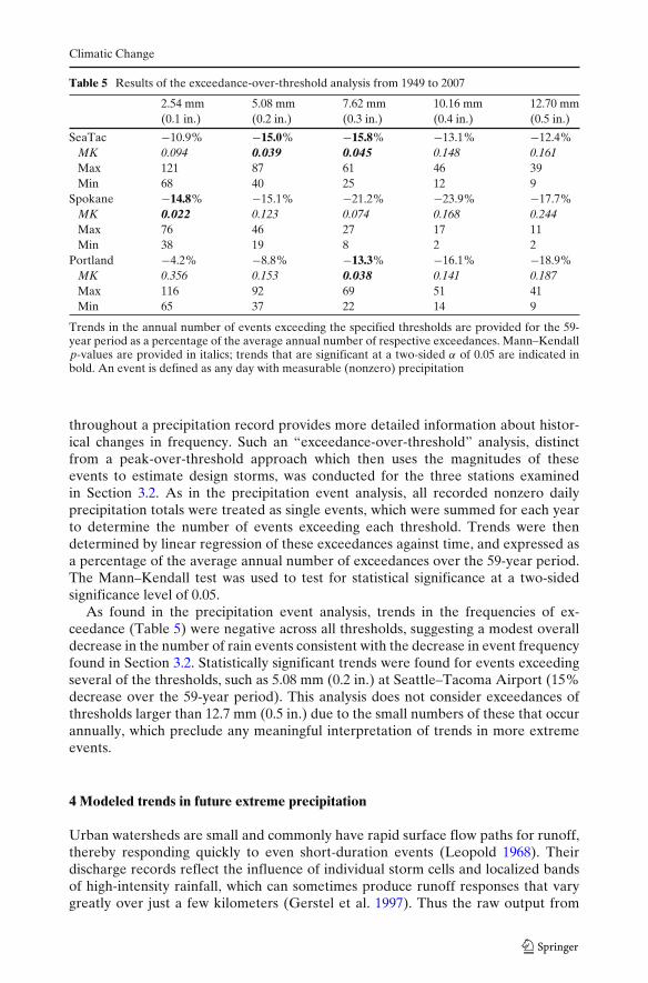
Table 5 Results of the exceedance-over-threshold analysis from 1949 to 2007

2.54 mm 5.08 mm 7.62 mm 10.16 mm 12.70 mm(0.1 in.) (0.2 in.) (0.3 in.) (0.4 in.) (0.5 in.)

SeaTac −10.9% −15.0% −15.8% −13.1% −12.4%MK 0.094 0.039 0.045 0.148 0.161Max 121 87 61 46 39Min 68 40 25 12 9

Spokane −14.8% −15.1% −21.2% −23.9% −17.7%MK 0.022 0.123 0.074 0.168 0.244Max 76 46 27 17 11Min 38 19 8 2 2

Portland −4.2% −8.8% −13.3% −16.1% −18.9%MK 0.356 0.153 0.038 0.141 0.187Max 116 92 69 51 41Min 65 37 22 14 9

Trends in the annual number of events exceeding the specified thresholds are provided for the 59-year period as a percentage of the average annual number of respective exceedances. Mann–Kendallp-values are provided in italics; trends that are significant at a two-sided α of 0.05 are indicated inbold. An event is defined as any day with measurable (nonzero) precipitation

throughout a precipitation record provides more detailed information about histor-ical changes in frequency. Such an “exceedance-over-threshold” analysis, distinctfrom a peak-over-threshold approach which then uses the magnitudes of theseevents to estimate design storms, was conducted for the three stations examinedin Section 3.2. As in the precipitation event analysis, all recorded nonzero dailyprecipitation totals were treated as single events, which were summed for each yearto determine the number of events exceeding each threshold. Trends were thendetermined by linear regression of these exceedances against time, and expressed asa percentage of the average annual number of exceedances over the 59-year period.The Mann–Kendall test was used to test for statistical significance at a two-sidedsignificance level of 0.05.

As found in the precipitation event analysis, trends in the frequencies of ex-ceedance (Table 5) were negative across all thresholds, suggesting a modest overalldecrease in the number of rain events consistent with the decrease in event frequencyfound in Section 3.2. Statistically significant trends were found for events exceedingseveral of the thresholds, such as 5.08 mm (0.2 in.) at Seattle–Tacoma Airport (15%decrease over the 59-year period). This analysis does not consider exceedances ofthresholds larger than 12.7 mm (0.5 in.) due to the small numbers of these that occurannually, which preclude any meaningful interpretation of trends in more extremeevents.

4 Modeled trends in future extreme precipitation

Urban watersheds are small and commonly have rapid surface flow paths for runoff,thereby responding quickly to even short-duration events (Leopold 1968). Theirdischarge records reflect the influence of individual storm cells and localized bandsof high-intensity rainfall, which can sometimes produce runoff responses that varygreatly over just a few kilometers (Gerstel et al. 1997). Thus the raw output from

Climatic Change

global climate models (GCMs), on which most assessments of future climate arebased, is not directly useable because the model grid resolution (100 s of km) is muchtoo coarse. For this reason, we instead used the two RCM simulations reported bySalathé et al. (2010) that produced downscaled GCM output at hourly aggregationswith spatial resolutions of 20 and 36 km (12.4 and 22.3 miles; see Leung et al. 2006;Salathe et al. 2008, 2010 for details). Although these spatial and temporal scalesare not ideal for capturing the behavior of urban runoff response, the use of RCMsimulations to estimate annual maximum series of precipitation (as opposed to peak-over-threshold extremes only) represents a significant advance in understandingprecipitation at the local scales at which watersheds respond to intense rainfall.

The two RCM simulations use different IPCC (2007b) GCM outputs as theirboundary conditions. Because the GCMs each predict future climate differently, andalso use slightly different global emissions scenarios, it is expected that they will alsodiffer in their projections of future climate. Ideally, a multimodel ensemble at theregional scale, which would parallel that used for regional hydrologic analysis (e.g.,Vano et al. 2010a, b), would be available for our analyses. At present, however, thisstrategy is not computationally feasible (each of the two RCM simulations requiredseveral months of computer time). Thus, the results presented here can offer a senseof the likely direction and general magnitude of future changes in precipitationextremes, but reducing their substantial uncertainties must await additional RCMsimulations that can be linked to the many other GCMs presently in existence.

4.1 RCM summary

The two GCMs that were used to provide boundary conditions for the RCMsimulations were the Community Climate System Model version 3.0 (CCSM3) withthe IPCC A2 emissions scenario, and the Max Planck Institute’s ECHAM5 withthe IPCC A1B emissions scenario (Table 6). During the first half of the 21stcentury, atmospheric CO2 concentrations are similar in both the A2 and the A1Bemissions scenarios, and so differences in the RCM simulation results are mostlydue to differences in the GCMs. Differences in spatial resolution may also influencethe results in ways that remain to be systematically explored. Both CCSM3 andECHAM5 are considered to be in the middle of the range of existing GCMs in theirprojections of precipitation for the Pacific Northwest (Mote et al. 2005).

The RCM used to downscale both GCMs was the Weather Research and Fore-casting (WRF) mesoscale climate model (http://www.wrf-model.org) developed atthe National Center for Atmospheric Research (NCAR). The CCSM3/A2 WRFsimulation was performed on a grid spacing of 20 km (12.4 miles), while the

Table 6 Summary of emission scenarios, GCMs, and geographic coordinates of the downscaledprecipitation records used for this study

IPCC Global Regional RCM grid spacing Lat-Long Coordinates of RCMEmissions Circulation Climate for Washington output used for hydrologicScenario Model (GCM) Model (RCM) State simulation modeling (see Fig. 4)

A2a CCSM3 WRF 20 km (12.4 miles) 47.525 ◦N 122.287 ◦WA1Bb ECHAM5 WRF 36 km (22.3 miles) 47.500 ◦N 122.345 ◦WaA2 simulations performed by Pacific Northwest National LaboratoriesbA1B simulations performed by UW-CIG

http://www.wrf-model.org

Climatic Change

ECHAM5/A1B WRF simulation had a grid spacing of 36 km (22.3 miles). Bothmodel simulations covered the time periods 1970–2000 (the “historical” period)and 2020–2050 (the “future” period), from which hourly precipitation data wereextracted. Annual maxima were derived from these “raw” data at grid points neareach of the three airports in the three urban regions (Puget Sound, Spokane, andVancouver–Portland). Statistical significance for differences in distributions wasdetermined using the Kolmogorov–Smirnov test, for differences in means using theWilcoxon rank-sum test, and for trends in the entire time series using the Mann–Kendall test, all at a two-sided significance level of 0.05.

Changes in average annual maxima between the two time periods are reportedin Table 7. While there was a greater number of increases than decreases, themagnitudes of the changes vary considerably across locations and simulations.Statistically significant changes were found for the Puget Sound region for bothsimulations, for Spokane for the CCSM3/A2 simulation for 3-h storms and for theECHAM5/A1B simulation for 24-h storms, and for Vancouver–Portland for theCCSM3/A2 simulation for 1-, 2-, and 3-h storms. Curiously, the intensities of shorterduration storms for Puget Sound and Spokane are projected to increase under theCCSM3/A2 simulations but decrease for the ECHAM5/A1B simulations.

A closer inspection of results for the CCSM3/A2 simulations revealed that,particularly for the Puget Sound region, the vast majority of modeled future annualmaxima are projected to occur in the month of November, a finding that was notreplicated in the ECHAM5/A1B simulations. Quality control checks demonstratedthat these elevated November projections were indeed present in the underlying

Table 7 Changes in the average modeled empirical annual maxima from 2020 to 2050 relative to theaverage modeled empirical annual maxima from 1970 to 2000, using raw RCM data

CCSM3/A2 ECHAM5/A1B

SeaTac Spokane Portland SeaTac Spokane Portland

1-h +16.2% +10.3% +10.5% −4.6% −6.6% +2.1%2-h +16.9% +5.9% +7.0% −4.3% −6.4% +3.9%3-h +17.5% +6.3% +6.5% −4.0% −5.8% +2.9%6-h +18.3% +5.4% +3.6% +3.6% −1.7% +1.2%12-h +15.9% +5.5% −0.5% +9.1% +12.1% +2.1%24-h +18.7% +3.9% +4.8% +14.9% +22.2% +2.0%2-day +11.2% +4.2% +2.0% +13.8% +16.0% +3.1%5-day +6.3% +3.2% +9.0% +12.2% +8.8% +4.6%10-day +9.0% +2.3% +7.5% +7.2% +8.9% +11.5%

CCSM3/A2 SeaTac 1-h +16.2% KS 0.014 rs 0.011 MK 0.015CCSM3/A2 SeaTac 2-h +16.9% KS 0.062 rs 0.013 MK 0.027CCSM3/A2 SeaTac 3-h +17.5% KS 0.030 rs 0.007 MK 0.020CCSM3/A2 SeaTac 6-h +18.3% KS 0.120 rs 0.019 MK 0.116CCSM3/A2 Spokane 3-h +6.3% KS 0.120 rs 0.128 MK 0.044CCSM3/A2 Portland 1-h +10.5% KS 0.120 rs 0.044 MK 0.004CCSM3/A2 Portland 2-h +7.0% KS 0.062 rs 0.076 MK 0.007CCSM3/A2 Portland 3-h +6.5% KS 0.062 rs 0.078 MK 0.009ECHAM5/A1B SeaTac 24-h +14.9% KS 0.006 rs 0.022 MK 0.045ECHAM5/A1B SeaTac 2-day +13.8% KS 0.030 rs 0.034 MK 0.072ECHAM5/A1B Spokane 24-h +22.2% KS 0.013 rs 0.023 MK 0.049

Statistically significant changes are indicated in bold and provided at bottom, as in Table 2

Climatic Change

GCM, but that they originated from the one ensemble member with the greatestdivergence from the ensemble mean, which indicates more modest changes inautumn precipitation. Thus, these particular results must be interpreted as thecombined influence of systematic climate change and internal climate variability.This result emphasizes the need to utilize a broader cross-section of GCMs andensemble members in a more comprehensive analysis, notwithstanding the consid-erable computational expense that this implies. For a more complete discussion, seeSalathé et al. (2010).

As a means of further interpreting the calculated changes, we performed aminimum detectable difference (MDD) analysis for each model run/duration combi-nation. The MDD is the smallest statistically significant change that can be detectedby a test of a specified power, given the sample size and underlying distribution of theobservations (characterized in our case by the mean and variance). For this analysis,we assumed that the population was normally distributed, with changes estimatedusing the Student’s t-statistic to approximate the MDD (see, e.g., Lettenmaier 1976,who also shows that results of the Mann–Kendall test are similar to those of the t-testwhen the underlying distribution is normal). We first determined the post-hoc powerof the t-test assuming a two-sided α of 0.05 and the actual sample’s combined size,variance, and detected change in average annual maxima (as reported in Table 7).Next, we calculated the MDD of the t-test, again assuming a two-sided α of 0.05 andthe actual sample’s combined size and variance, but this time with the power takento be 0.5. Finally, we estimated the combined sample size that would be requiredto demonstrate statistical significance for the detected change in average annualmaxima, given the sample’s variance, and assuming a two-sided α of 0.05 and powerof 0.5.

The results of the MDD analysis (Table 8) offer further explanation for thepatterns presented in Table 7. With the exception of the CCSM3/A2 simulationat Seattle–Tacoma Airport, which resulted in a greater number of statistically sig-nificant results for the reasons discussed above, the majority of post-hoc powers weredetermined to be largely deficient. In most cases, MDDs were likewise determined tobe greater than the detected changes in average annual maxima provided in Table 7.The underlying reason is that the sample variances were too large for the samplesizes available. Stated otherwise, most of the required sample sizes were considerablylarger than the 62 years of simulations available for our analyses.

4.2 Bias correction and statistical downscaling (BCSD)

Although the raw output from the RCM provides a broadly recognizable pattern ofrainfall, even a cursory comparison of simulated and gauged records shows obviousdisparities in both the frequency of rainfall events and the total amount of recordedprecipitation. For example, from 1970 to 2000, the CCSM3/A2 simulation at the gridcenter closest to Seattle–Tacoma Airport resulted in 11,734 h of nonzero precipi-tation for a total of 5,720 mm (225 in.) during the month of January (average of379 h and 185 mm [7.3 in.]), while the Seattle–Tacoma Airport gauge recorded only4,144 h of nonzero precipitation for a total of 4,110 mm (162 in.; average of 134 h and133 mm [5.2 in.]). Thus, if the RCM data are to be used as forcings for a hydrologicmodel, they must first be bias-corrected. We describe a procedure for doing so in theremainder of this section, which focuses on the central Puget Sound region.

Climatic Change

Table 8 Results of the MDD analysis

CCSM3/A2 ECHAM5/A1B

SeaTac Spokane Portland SeaTac Spokane Portland

1-h power 0.63 0.14 0.30 0.07 0.11 0.05MDD 13.9% 22.9% 14.2% 17.1% 17.6% 13.2%nmin 56 138 84 228 160 386

2-h power 0.64 0.08 0.17 0.07 0.11 0.09MDD 14.4% 20.2% 13.8% 17.0% 16.6% 12.8%nmin 54 208 122 236 158 198

3-h power 0.65 0.09 0.15 0.07 0.11 0.07MDD 14.6% 19.2% 13.7% 16.5% 14.9% 12.4%nmin 52 186 128 250 158 260

6-h power 0.61 0.08 0.07 0.07 0.04 0.04MDD 16.1% 19.5% 14.2% 14.6% 14.1% 11.7%nmin 56 218 236 244 486 590

12-h power 0.44 0.08 0.03 0.25 0.33 0.05MDD 17.2% 19.7% 15.9% 13.7% 15.6% 12.6%nmin 68 220 1826 92 80 360

24-h power 0.52 0.06 0.09 0.48 0.61 0.05MDD 18.3% 20.3% 15.1% 15.2% 19.4% 13.7%nmin 62 316 192 64 54 408

2-day power 0.28 0.06 0.05 0.34 0.40 0.06MDD 15.9% 19.4% 13.6% 17.5% 18.5% 15.4%nmin 88 276 402 78 72 302



The top row of each cell is the post-hoc power of a t-test assuming a two-sided α of 0.05 and theactual sample’s combined size, sample variance, and detected change in average annual maxima,as reported in Table 7. The middle row is the MDD of a t-test, again assuming a two-sided α of0.05 and the actual sample’s combined size and variance, with power of 0.5. The bottom row is thecombined sample size that would be required for the detected change in average annual maxima tobe statistically significant, given the sample’s variance, and assuming a two-sided α of 0.05 and powerof 0.5. Results corresponding to detected changes that were statistically significant are indicatedin bold

Methods of removing systematic bias in RCM output are described by Wood et al.(2002) and Payne et al. (2004). We generalized their procedure, which is based onprobability mapping as described by Wilks (2006), to apply to precipitation extremes.The objective of the procedure is to transform the modeled data so that they havethe same probability distributions as their observed counterpart.

Bias correction was applied to the simulation record for the grid point fromeach of the two downscaled hourly WRF time series (1970–2000 and 2020–2050)that was closest to Seattle–Tacoma Airport (Fig. 4). For the RCM run forced bythe CCSM3/A2 simulation (hereafter referred to as the “CCSM3” run), the grid

Climatic Change

Fig. 4 Locations of the twogrid points used for BCSD,shown in relation to SeaTacAirport and the ThorntonCreek and Juanita Creekwatersheds (see Section 5).Figure: Robert Norheim

point employed was 47.525◦ N, 122.287◦ W, corresponding to a location about9 km (5.6 miles) NNE of Seattle–Tacoma Airport. For the RCM run forced by theECHAM5/A1B simulation (hereafter referred to as the “ECHAM5” run), the gridpoint employed was 47.500◦ N, 122.345◦ W, corresponding to a location about 7 km(4.3 miles) NNW of Seattle–Tacoma Airport. For purposes of comparison, a separatebias correction was performed for each run at their next grid point to the south;results were very similar and are not reported here.

The first step in the procedure was to truncate simulated data for the 1970–2000period so that each month had the same number of nonzero hourly values as theobserved data from the Seattle–Tacoma Airport gauge, which were the same dataused in the historical analyses described in Section 3. This was done to correctfor oversimulation by the RCM of small amounts (sometimes termed the “climatemodel drizzle problem”). Simulated data for the future period (2020–2050) weresimilarly truncated, using the same threshold hourly values resulting from matchingthe number of nonzero past values to that which was observed. Thus, using theexample provided above, the 7,590 h (i.e., 11,734–4,144 h) containing the smallestamounts of nonzero precipitation were eliminated from the 1970–2000 simulatedrecord for the month of January, coinciding with a truncation threshold of 0.3 mm(0.012 in.). Any hour during the month of January during the 2020–2050 simulated

Climatic Change

record with a nonzero precipitation of less than 0.3 mm (0.012 in.) was also eliminated(6,824 out of 10,322 h).

Bias correction was then achieved by replacing RCM values with values havingthe same nonexceedence probabilities, with respect to the observed climatology, thatthe original RCM values had with respect to the RCM climatology. The procedurewas first performed at a monthly time interval to ensure that the dramatic seasonaldifferences that characterize rainfall in western Washington were preserved andrepresented accurately. Monthly totals were calculated (by year), and the Weibullplotting position was employed to map those totals from the simulated empiricalcumulative distribution function (eCDF) to monthly totals from the observed eCDF.Next, simulated hourly values were rescaled to add up to the new monthly totals.The procedure was then repeated; the new hourly values were mapped from theireCDF to the hourly values from the observed eCDF and once again rescaled tomatch the monthly totals derived in the first mapping step. Values that fell outsidethe range of the simulated climatology, but within 3.5 standard deviations of theclimatological mean, were corrected by assuming a lognormal distribution. Thosethat fell outside of 3.5 standard deviations of the climatological mean were correctedby scaling the mean of the observed climatology by its ratio with the mean of thesimulated climatology.

The resulting eCDFs for historical and future climate were tested for significanceof differences using the Kolmogorov–Smirnov, Wilcoxon rank-sum, and Mann–Kendall tests at a two-sided α of 0.05. Overall, average biases in empirical annualmaxima were reduced from −22.2% to +3.1% for the ECHAM5 run, and from+9.6% to +2.5% for the CCSM3 run (Table 9). Changes in the raw annual maximabetween the 1970–2000 and 2020–2050 periods were largely preserved, although theprocedure did have the effect of making some of the changes under the CCSM3simulation more statistically significant. Under the ECHAM5 run, the correctedempirical annual maxima display a decrease between the two 30-year periods byan average of 5.8 to 6.3% for 1-, 2-, and 3-h durations, and an increase of 2.3 to14.1% for the remaining durations. For the CCSM3 run, the corrected empiricalannual maxima show an increase of 13.7 to 28.7% across all durations.

It is generally recognized that the downscaling problem is more complicated forprecipitation extremes than precipitation means, for the intuitive reason that mostextreme events tend to be concentrated on very small spatial scales, which are notwell represented in climate models. Because the magnitudes of our bias correctionsof simulated data is necessarily greater in the tails of the distributions than in themiddle, our analysis effectively accounts for this problem. That said, the procedureis not exact, and there are no doubt refinements that can still be made. However, theranges and medians of the modeled, bias-corrected maxima generally match thoseof the observed maxima for the historical period (1970–2000), as shown for the 24-hduration in Fig. 5.

5 Prediction of future changes in urban flood extremes

Although our analysis thus far has focused on changes in precipitation across themajor urban areas of Washington State, the direct relevance of these changesto stormwater infrastructure is best displayed through predictions of future

Climatic Change

Tab

le9

Res

ults

ofth

ebi

as-c

orre

ctio

npr

oced

ure

for

both

RC

Mru

nsat

Seat

tle–

Tac

oma

Air

port

CC

SM3/

A2

EC

HA

M5/

A1B

Bia

sC

hang

eB

ias

Cha

nge

Raw

Cor

Raw

Cor

Raw

Cor

Raw

Cor

1-h

−19.

2%−7

.3%

+16.

2%+1

4.3%

−33.

2%−1

3.4%

−4.6

%−6

.3%

2-h

−2.6

%+4

.1%

+16.

9%+2

2.8%

−21.

2%+3

.9%

−4.3

%−5

.8%

3-h

+2.4

%+6

.2%

+17.

5%+2

3.7%

−17.

3%+1

1.8%

−4.0

%−6

.3%

6-h

+8.8

%+6

.6%

+18.

3%+2

4.3%

−17.

3%+1

2.8%

+3.6

%+2

.3%

12-h

+12.

7%+4

.4%

+15.

9%+2

4.2%

−20.

6%+6

.8%

+9.1

%+8

.3%

24-h

+11.

0%−1

.9%

+18.

7%+2

8.7%

−22.

7%+3

.4%

+14.

9%+1

4.1%

2-da

y+1

9.4%

−1.1

%+1

1.2%

+24.

0%−2

2.7%

+1.2

%+1

3.8%

+14.

1%5-

day

+29.

0%+7

.1%

+6.3

%+1

3.7%

−22.

4%+1

.1%

+12.

2%+1

1.5%

10-d

ay+2

5.1%

+4.6

%+9

.0%

+18.

0%−2

2.4%

+0.3

%+7

.2%

+7.8

%A

vera

ge+9

.6%

+2.5

%–

–−2

2.2%

+3.1

%–

–

CC

SM3/

A2

1-h

(raw

)+1

6.2%

KS

0.01

4rs

0.01

1M

K0.

015

1-h

(cor

)+1

4.3%

KS

0.00

2rs

0.01

3M

K0.

003

CC

SM3/

A2

2-h

(raw

)+1

6.9%

KS

0.06

2rs

0.01

3M

K0.

027

2-h

(cor

)+2

2.8%

KS

0.00

1rs

0.00

1M

K0.

001

CC

SM3/

A2

3-h

(raw

)+1

7.5%

KS

0.03

0rs

0.00

7M

K0.

020

3-h

(cor

)+2

3.7%

KS

0.00

2rs

0.00

0M

K0.

001

CC

SM3/

A2

6-h

(raw

)+1

8.3%

KS

0.12

0rs

0.01

9M

K0.

116

6-h

(cor

)+2

4.3%

KS

0.03

0rs

0.00

5M

K0.

044

CC

SM3/

A2

12-h

(raw

)+1

5.9%

KS

0.21

6rs

0.07

6M

K0.

331

12-h

(cor

)+2

4.2%

KS

0.03

0rs

0.00

9M

K0.

155

CC

SM3/

A2

24-h

(raw

)+1

8.7%

KS

0.21

6rs

0.05

2M

K0.

291

24-h

(cor

)+2

8.7%

KS

0.01

3rs

0.00

3M

K0.

085

CC

SM3/

A2

2-da

y(r

aw)

+11.

2%K

S0.

120

rs0.

143

MK

0.33

12-

day

(cor

)+2

4.0%

KS

0.01

3rs

0.00

4M

K0.

099

CC

SM3/

A2

10-d

ay(r

aw)

+9.0

%K

S0.

216

rs0.

177

MK

0.57

210

-day

(cor

)+1

8.0%

KS

0.00

2rs

0.01

0M

K0.

078

EC

HA

M5/

A1B

24-h

(raw

)+1

4.9%

KS

0.00

6rs

0.02

2M

K0.

045

24-h

(cor

)+1

4.1%

KS

0.06

2rs

0.04

0M

K0.

034

EC

HA

M5/

A1B

10-d

ay(r

aw)

+13.

8%K

S0.

030

rs0.

034

MK

0.07

210

-day

(cor

)+1

4.1%

KS

0.00

6rs

0.02

3M

K0.

033

The

repo

rted

bias

esar

eth

ose

ofth

eav

erag

em

odel

edem

piri

cala

nnua

lmax

ima

(bot

hra

wan

dco

rrec

ted)

rela

tive

toth

eav

erag

eob

serv

edem

piri

cala

nnua

lmax

ima

from

1970

to20

00.T

here

port

edch

ange

sar

eth

ose

ofth

eav

erag

em

odel

edem

piri

cala

nnua

lmax

ima

from

2020

to20

50re

lati

veto

the

aver

age

mod

eled

empi

rica

lan

nual

max

ima

from

1970

to20

00,u

sing

both

raw

and

corr

ecte

dda

ta.S

tati

stic

ally

sign

ific

ant

chan

ges

are

indi

cate

din

bold

wit

hte

stst

atis

tics

prov

ided

atbo

ttom

,as

inT

able

2

Climatic Change

Fig. 5 Box-whisker plots ofobserved and modeled (rawand bias-corrected) 24-hannual maxima atSeattle–Tacoma Airport forthe CCSM3/A1 scenario(upper) and theECHAM5/A1B scenario(lower). Red line denotes themedian, solid box denotes therange from 25th to 75thpercentiles, and whiskersdenote the range of the rest ofthe data. Plus signs denoteoutliers more than 1.5 timesthe interquartile range fromthe top or bottom of the box

24-Hour Annual Maxima for CCSM3/A2

24-Hour Annual Maxima for ECHAM5/A1B

150

125

100

Pre

cipi

tatio

n (m

m)

Pre

cipi

tatio

n (in

.)P

reci

pita

tion

(in.)

Pre

cipi

tatio

n (m

m)

75

50

25

0

6

5

4

3

2

1

0

6

5

4

3

2

1

0

150

125

100

75

50

25

0

70-00 (obs) 70-00 (raw) 70-00 (cor) 20-50 (raw) 20-50 (cor)

70-00 (obs) 70-00 (raw) 70-00 (cor) 20-50 (raw) 20-50 (cor)

streamflows. As case studies, we selected two Seattle-area watersheds (Fig. 4),Thornton Creek in the City of Seattle and Juanita Creek in the City of Kirklandand adjacent unincorporated King County, because they encompass physical andland-use characteristics typical of the central Puget Lowland. The Thornton Creekwatershed is Seattle’s largest, with approximately 2870 ha (7090 ac) of mixed com-mercial and residential land use. Juanita Creek is a mixed-land-use 1760-ha (4350-ac)watershed that drains to the eastern shore of Lake Washington; its land cover is 34%effective impervious with 30% forest cover.

Hydrologic simulations of streamflows in these two watersheds were generatedby the Hydrologic Simulation Program-Fortran (HSPF; Bicknell et al. 1996). HSPF,which was developed under contract to and is maintained by the U.S. EnvironmentalProtection Agency, is a lumped-parameter model that simulates discharge at user-selected points along a channel network from a time series of meteorologicalvariables (notably, rainfall, temperature, and solar radiation) and a characterizationof hydrologic variables (such as infiltration capacity and soil water-holding capacity)

Climatic Change

that are typically averaged over many hectares or square kilometers. HSPF hasbeen widely applied across western Washington since its first regional applicationin the mid-1980s (King County 1985), and the procedures for model set-up, initialparameter selection, and calibration are well established for the region (Dinicolaet al. 1990, 2001).

The BCSD precipitation data for the periods 1970–2000 and 2020–2050 wereinput to HSPF to reconstitute historical streamflows and predict future streamflowsin the Thornton Creek and Juanita Creek watersheds using the RCM grid pointspreviously discussed (see Section 4.2; Table 6 and Fig. 4). Because the inputs to thehydrologic model for the two periods differed only in precipitation, any attributeof an altered hydrologic response that is not driven predominantly by rainfall (e.g.,the dependence of low-flow extremes on evapotranspiration rates) would not beplausibly represented and has not been explored here. These two case studies,however, offer some guidance as to whether predicted runoff changes in urban andsuburban areas present any critical areas of concern for stormwater managers.

5.1 Results

To parallel the approach of the BCSD analysis, HSPF was first used to evaluatedifferences between 1970–2000 simulated flows resulting from forcing HSPF withthe historical rainfall record and the BCSD rainfall. Results from both the ThorntonCreek and Juanita Creek modeling runs suggest streamflow biases of the samemagnitude or less than those from the direct comparison of observed and simulatedrainfall records (see Tables 10, 11, 12 and Fig. 6). For the exploratory purposes thatmotivated the modeling, these differences were judged acceptable.

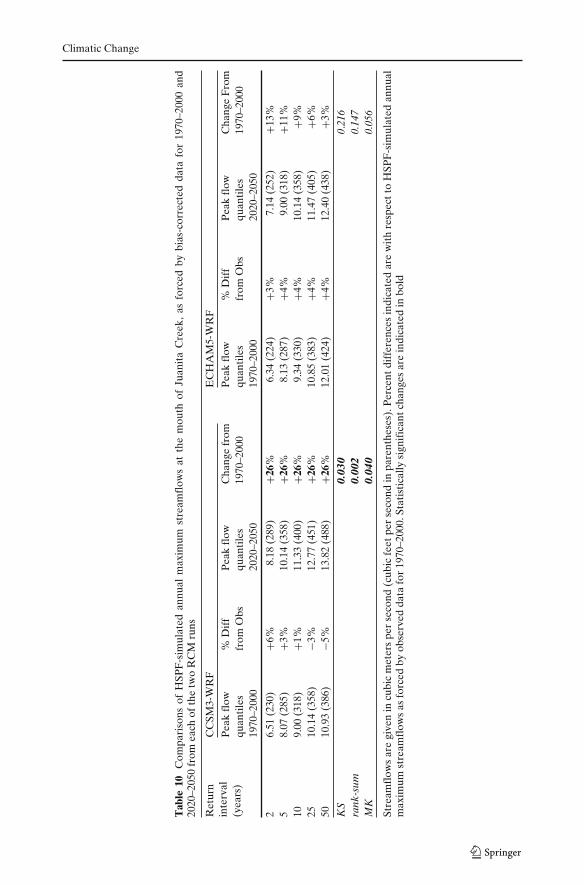
Streamflows were then simulated for both watersheds and each of the two RCMruns using the BCSD rainfall for the periods 1970–2000 and 2020–2050. Log-Pearsontype 3 distributions were fitted to the resulting annual maxima, as recommended byUS federal agencies for flood frequency analyses (IACWD 1982), and changes weretested for statistical significance using the Kolmogorov–Smirnov, Wilcoxon rank-sum, and Mann–Kendall tests at a two-sided α of 0.05. Results at the mouths of bothwatersheds (Tables 10 and 11) indicate increases in streamflows for both RCM runsat all recurrence intervals. While these increases are smaller at the mouth of JuanitaCreek, this is most likely the consequence of an extensive wetlands complex thatattenuates peak flows in that watershed.

Despite this relative uniformity, however, not every scenario is equally consistent.Statistically significant results using CCSM3-generated precipitation are systemati-cally greater than those using ECHAM5, which are not statistically significant. Eventhe relatively large increases at Thornton Creek under ECHAM5 are insignificant,due to the large variance present in those particular data. In addition, in the HSPFresults for Kramer Creek, a 45-ha (110-ac) mixed commercial and residential sub-watershed that constitutes less than 2% of the Thornton Creek watershed area,simulated changes in peak flow differ in sign between the two scenarios. For theCCSM3-driven simulations, 2-year through 50-year peak flows are projected torise by as much as 25% while the ECHAM5-driven simulations mostly indicatesmall declines (Table 12). Although they constitute only a single example, thesesubstantially different results suggest that the present state of understanding in the

Climatic Change

Tab

le10

Com

pari

sons

ofH

SPF

-sim

ulat

edan

nual

max

imum

stre

amfl

ows

atth

em

outh

ofJu

anit

aC

reek

,as

forc

edby

bias

-cor

rect

edda

tafo

r19

70–2

000

and

2020

–205

0fr

omea

chof

the

two

RC

Mru

ns

Ret

urn

CC

SM3-

WR

FE

CH

AM

5-W

RF

inte

rval

Pea

kfl

ow%

Dif

fP

eak

flow

Cha

nge

from

Pea

kfl

ow%

Dif

fP

eak

flow

Cha

nge

Fro

m(y

ears

)qu

anti

les

from

Obs

quan

tile

s19

70–2

000

quan

tile

sfr

omO

bsqu

anti

les

1970

–200

019

70–2

000

2020

–205

019

70–2

000

2020

–205

0

26.

51(2

30)

+6%

8.18

(289

)+2

6%6.

34(2

24)

+3%

7.14

(252

)+1

3%5

8.07

(285

)+3

%10

.14

(358

)+2

6%8.

13(2

87)

+4%

9.00

(318

)+1

1%10

9.00

(318

)+1

%11

.33

(400

)+2

6%9.

34(3

30)

+4%

10.1

4(3

58)

+9%

2510

.14

(358

)−3

%12

.77

(451

)+2

6%10

.85

(383

)+4

%11

.47

(405

)+6

%50

10.9

3(3

86)

−5%

13.8

2(4

88)

+26%

12.0

1(4

24)

+4%

12.4

0(4

38)

+3%

KS

0.03

00.

216

rank

-sum

0.00

20.

147

MK

0.04

00.

056

Stre

amfl

ows

are

give

nin

cubi

cm

eter

spe

rse

cond

(cub

icfe

etpe

rse

cond

inpa

rent

hese

s).P

erce

ntdi

ffer

ence

sin

dica

ted

are

wit

hre

spec

tto

HSP

F-s

imul

ated

annu

alm

axim

umst

ream

flow

sas

forc

edby

obse

rved

data

for

1970

–200

0.St

atis

tica

llysi

gnif

ican

tcha

nges

are

indi

cate

din

bold

Climatic Change

Tab

le11

Com

pari

sons

ofH

SPF

-sim

ulat

edan

nual

max

imum

stre

amfl

ows

atth

em

outh

ofT

horn

ton

Cre

ek,a

sfo

rced

bybi

as-c

orre

cted

hour

lypr

ecip

itat

ion

data

for

1970

–200

0an

d20

20–2

050

from

each

ofth

etw

oR

CM

runs

Ret

urn

CC

SM3-

WR

FE

CH

AM

5-W

RF

inte

rval

Pea

kfl

ow%

Dif

fP

eak

flow

Cha

nge

from

Pea

kfl

ow%

Dif

fP

eak

flow

Cha

nge

from

(yea

rs)

quan

tile

sfr

omO

bsqu

anti

les

1970

–200

0qu

anti

les

from

Obs

quan

tile

s19

70–2

000

1970

–200

020

20–2

050

1970

–200

020

20–2

050

23.

34(1

18)

+17%

5.30

(187

)+5

9%3.

03(1

07)

+6%

3.79

(134

)+2

5%5

5.27

(186

)+1

4%8.

27(2

92)

+57%

4.90

(173

)+6

%6.

37(2

25)

+30%

106.

74(2

38)

+10%

10.3

1(3

64)

+53%

6.43

(227

)+5

%8.

38(2

96)

+30%

258.

83(3

12)

+6%

12.9

7(4

58)

+47%

8.75

(309

)+5

%11

.30

(399

)+2

9%50

10.5

6(3

73)

+2%

14.9

8(5

29)

+42%

10.7

9(3

81)

+5%

13.7

3(4

85)

+27%

KS

0.00

30.

951

rank

-sum

0.00

10.

624

MK

0.00

50.

399

Stat

isti

cally

sign

ific

antc

hang

esar

ein

dica

ted

inbo

ld

Climatic Change

Tab

le12

Com

pari

sons

ofH

SPF

-sim

ulat

edan

nual

max

imum

stre

amfl

ows

atth

em

outh

ofK

ram

erC

reek

,as

forc

edby

bias

-cor

rect

edho

urly

prec

ipit

atio

nda

tafo

r19

70–2

000

and

2020

–205

0fr

omea

chof

the

two

RC

Mru

ns

Ret

urn

CC

SM3-

WR

FE

CH

AM

5-W

RF

inte

rval

Pea

kfl

ow%

Dif

fP

eak

flow

Cha

nge

from

Pea

kfl

ow%

Dif

fP

eak

flow

Cha

nge

from

(yea

rs)

quan

tile

sfr

omO

bsqu

anti

les

1970

–200

0qu

anti

les

from

Obs

quan

tile

s19

70–2

000

1970

–200

020

20–2

050

1970

–200

020

20–2

050

20.

20(7

.0)

+4%

0.25

(8.8

)+2

5%0.

19(6

.6)

−1%

0.19

(6.7

)0%

50.

24(8

.6)

+4%

0.30

(10.

6)+2

5%0.

24(8

.3)

0%0.

24(8

.3)

0%10

0.27

(9.5

)+1

%0.

33(1

1.7)

+22%

0.27

(9.4

)0%

0.26

(9.3

)−4

%25

0.30

(10.

6)0%

0.36

(12.

8)+2

0%0.

31(1

0.9)

+3%

0.29

(10.

4)−6

%50

0.32

(11.

4)−1

%0.

38(1

3.5)

+19%

0.34

(12.

0)+4

%0.

32(1

1.2)

−8%

KS

0.00

10.

951

rank

-sum

0.00

10.

898

MK

0.00

10.

455

Stat

isti

cally

sign

ific

antc

hang

esar

ein

dica

ted

inbo

ld

Climatic Change

Annual Peak Frequency Analysis. 1 hour moving average.Fit Type:Log Pearson III distribution using the method of Bulletin 17B, Weibul Plottng Position

Ret Period-->

SEA HIST SB THORNTON CK, SEATAC 1970-2000

A1B HIST SB THORNTON CK, ECHAM5-A1B 1970-2000A2 HIST SB THORNTON CK, CCSM3-A2 1970-2000

2 5 10 100 5002

75

3

101

99.8 99 90 80 50

Percent Chance Exceedance

Dis

char

ge (

cms)

20 10 0.21

Ret Period SEA HIST500.100.10.

5.2.

17.536913.50338.58947.21555.3051

Ret Period A2 HIST500.100.10.

5.2.

14.528212.08778.60847.48735.7652

Ret Period A1B HIST500.100.10.

5.2.

15.092912.06928.13356.96435.2675

Fig. 6 Example Flood Frequency Curves for the South Branch of Thornton Creek (930-ha [2300-ac]drainage area), comparing HSPF-simulated results for the period 1970–2000 driven by the Seattle–Tacoma Airport rainfall record (red line and symbols) with the results driven by the BCSD rainfallfrom the two alternative climate scenarios (green and blue)

implications of projected changes in precipitation extremes is still highly uncertain,at least for small urban drainage basins of this scale.

We explored predicted changes in runoff characteristics for both RCM runs forflow metrics other than peak annual discharge, using selected indices of hydrologicalteration (IHA) that have likely ecological influence (Konrad and Booth 2002;Richter et al. 1996). These include indices that assess the time of year for averageor extreme flow events, the frequency and duration of flow pulses, and the rate andfrequency of change in flow conditions. In general, these metrics did not changenearly as much as did the peak annual discharge (e.g., Table 10). As an example,the results for high pulse start date at Juanita Creek (Fig. 7) are relatively consistent:only modest differences are apparent between the two scenarios, and very limiteddifferences between the two simulation periods.

In contrast, analysis of a common measure of stream-channel erosivity (aggregateduration of flow above a threshold discharge) indicates systematic changes betweenthe present and future periods. The threshold discharge assumed in this study is50% of the peak 2-year flow for the period 1970–2000, which has been foundto be a regionally credible index value for initiation of sediment transport in analluvial gravel-bed channel (Booth and Jackson 1997). A single value, derivedfrom the average of the three 1970–2000 simulations, was used as this “thresholddischarge” for all duration analyses at a given stream location. Both RCM-driven

Climatic Change

A1B High Pulse Start Empirical CDFA1B High Pulse Start

ExceedanceYear

ExceedanceYear

A2 High Pulse Start Empirical CDFA2 High Pulse Start

340

330

320

310

300

290

280

270

330

320

310

300

290

280

270

330

320

310

300

290

280

270

340

330

320

310

300

290

280

2701960 1980 2000 2020 2040 2060 0 0.2 0.4 0.6 0.8 1

0 0.2 0.4 0.6 0.8 11960 1980 2000 2020 2040 2060

Julia

n D

ayJu

lian

Day

Julia

n D

ayJu

lian

Day

Fig. 7 Example of an IHA metric (high pulse start date) as simulated by the two RCM-based HSPFsimulations for the periods 1970–2000 and 2020–2050 at the mouth of Juanita Creek. Differencesbetween models, or between periods, are neither systematic nor particularly large

simulations show consistent increases, with the largest change associated with thesmallest watershed area (Table 13). Similar to other results that compare simulated2020–2050 flows to those for 1970–2000, increases in erosivity predicted using theCCSM3 precipitation dataset are consistently more dramatic than those predictedusing the ECHAM5 dataset. In comparison to streamflow simulations driven by the

Table 13 Flow durations for Q > 50% of the 2-year discharge (percent of time exceedance), aspredicted by HSPF at four locations along the channel network of Thornton Creek

SeaTac historical CCSM3-WRF ECHAM5-WRF

1970–2000 (%) 1970–2000 2020–2050 Change 1970–2000 2020–2050 Change(%) (%) (%) (%) (%) (%)

Kramer Creek (45 ha [110 ac])0.23 0.28 0.58 +107 0.29 0.51 +76

South Branch Thornton Creek0.23 0.28 0.42 +50 0.29 0.34 +17

North Branch Thornton Creek0.36 0.45 0.66 +47 0.46 0.56 +22

Thornton Creek nr Mouth (2870 ha [7090 ac])0.19 0.24 0.38 +58 0.24 0.30 +25

The first column gives the time of exceedance using the historical record; the 1970–2000 column foreach GCM shows the same metric using the BCSD simulated record (with simulation results about1/3 higher, on average). The column labeled Change is the 2020–2050 value for this metric relative tothe 1970–2000 durations using the BCSD rainfall record

Climatic Change

historical 1970–2000 rainfall record, however, both RCM-driven simulations consis-tently overestimate high-flow durations by approximately one-third. Interestingly,the two different RCM-based simulations produce very consistent errors; apparentlythe bias-correction procedures do not adequately adjust the moderate levels ofprecipitation intensity that affect this flow statistic.

6 Discussion

Our analyses of historical precipitation yielded largely (statistically) inconclusivetrends in extreme precipitation over a range of durations during the past half-century,with substantial differences among the three major metropolitan areas. In the PugetSound region, statistically significant increases in annual maxima were observedat the 24-h duration, which is the interval most frequently used for the designof stormwater infrastructure. Annual maxima in the other two regions, however,displayed markedly different changes over the last 50 years, with mixed results inthe Spokane region and consistently negative changes in the Portland–Vancouverregion, none of which were statistically significant. Although prior studies havemostly focused on trends in the frequency of extreme events, and not in intensity aswe have done here, these results are consistent with those of Kunkel et al. (1999) andPryor et al. (2009), both of which found ambiguous trends in the Pacific Northwest, aswell as Madsen and Figdor (2007), who found statistically significant upward trendsin both Washington and Seattle but mixed trends in Oregon and Idaho.

Modeled trends in future precipitation extremes were generally more consistentthan in the historical analyses. Two different GCMs provided the coarse-scaleboundary conditions used to generate downscaled precipitation results, and bothagree in general trends. However, the precise levels of rainfall increases predicted bythe two models vary substantially, and inferred changes were difficult to distinguishfrom natural variability given the relatively short simulation periods. While thedifferences between the two sets of current and future climate simulations are largeenough to have potentially important consequences for the design of stormwaterfacilities, most are nonetheless not statistically significant.

Results of the hydrologic modeling on two urban watersheds in the central PugetSound region affirm and extend both the broad trends and the substantial uncertain-ties evident in the precipitation simulations. For the two watersheds modeled, thesimulations generally agree that peak discharges will increase, although the rangeof predicted change (from a slight decrease to a near-doubling, depending on theselected recurrence interval, watershed, and underlying GCM simulation) is muchtoo large to provide a basis for engineering design. The comparative simulationresults are most confounding for the smallest watershed areas, wherein even the netdirection of change (i.e., a future increase or a future decrease) is in part dependenton the choice of GCM.

7 Conclusions

Our objectives in this paper were to characterize past and future trends in precip-itation extremes across Washington State, with the ultimate goal of assessing the

Climatic Change

impacts of climate change on its stormwater infrastructure. Despite some uncertain-ties amongst the results of our study, we offer the following conclusions in summary:

• Few statistically significant changes in extreme precipitation have been observedto date in the state’s three major metropolitan areas, with the possible exceptionof the Puget Sound. Nonetheless, drainage infrastructure designed using mid-twentieth century rainfall records may be subject to a future rainfall regime thatdiffers from current design standards.

• Projections from two regional climate model (RCM) simulations generally indi-cate increases in extreme rainfall magnitudes throughout the state over the nexthalf-century, but their projections vary substantially by both model and region,and actual changes may be difficult to distinguish from natural variability.

• Hydrologic modeling of two urban creeks in central Puget Sound suggest overallincreases in peak annual discharge over the next half-century, but only thoseprojections resulting from one of the two RCM simulations are statisticallysignificant. Magnitudes of projected changes vary widely, depending on theparticular basin under consideration and the choice of the underlying globalclimate model.

Our assessment of future streamflows, and the magnitudes of peak discharges onwhich the design of stormwater infrastructure is based, suggests that concern overpresent design standards is warranted. However, because our analysis is based ononly two GCMs, it is at most suggestive. For a more complete understanding of howprecipitation extremes are likely to change in the future, the methods employed inthe precipitation distribution analysis should be used to explore a larger sample ofsimulated climate data. Additional model simulations, based on a larger ensemble ofGCMs and emission scenarios, will be required to develop a more robust set of con-clusions and provide additional information for evaluating alternative stormwater-facility design standards.

Acknowledgements This study was conducted under the auspices of the University ofWashington’s Climate Impacts Group, with additional support provided by Seattle Public Utilitiesand Northwest Hydraulic Consultants (to DH), King County Water and Land Resources Division(to JB), and Stillwater Sciences (to DBB). We thank Rob Norheim for providing the maps andLara Whitely Binder for reviewing an early draft of the paper. We would also like to acknowledgethe encouragement and insights of Paul Fleming and Gary Schimek (City of Seattle) and thecontributions of five anonymous reviewers, whose comments resulted in substantial improvements tothe paper. This publication is part of the Washington Climate Change Impacts Assessment, fundedby the 2007 Washington State Legislature through House Bill 1303. This publication is partiallyfunded by the NOAA Regional Integrated Sciences and Assessments program and the NOAAClimate Dynamics and Experimental Prediction/Applied Research Centers program under NOAACooperative Agreement No. NA17RJ1232 to the Joint Institute for the Study of the Atmosphereand Ocean (JISAO). This is JISAO Contribution #1796.

References

Bicknell BR et al (1996) Hydrological Simulation Program—Fortran: User’s manual for Release 11.US Environmental Protection Agency, Environmental Research Laboratory, Office of Researchand Development, Athens, Georgia

Booth DB, Jackson CR (1997) Urbanization of aquatic systems—degradation thresholds, stormwa-ter detention, and the limits of mitigation. J Am Water Resour Assoc 33(5):1077–1090

Choguill CL (1996) Ten steps to sustainable infrastructure. Habitat Int 20(3):389–404

Climatic Change

Denault C, Millar RJ, Lence BJ (2002) Climate change and drainage infrastructure capacity in anurban catchment. Annual conference of the Canadian Society for Civil Engineering, Montreal,Quebec, Canada

Dinicola et al (1990) Characterization and simulation of rainfall-runoff relations for headwater basinsin western King and Snohomish Counties, Washington. US Geological Survey Water-ResourcesInvestigation Report 89-4052

Dinicola et al (2001) Validation of a numerical modeling method for simulating rainfall-runoff rela-tions for headwater basins in western King and Snohomish Counties, Washington. US GeologicalSurvey Water-Supply Paper 2495

Efron B (1979) Bootstrap methods: another look at the jackknife. Ann Stat 7(1):1–26Fowler HJ, Kilsby CG (2003) A regional frequency analysis of United Kingdom extreme rainfall

from 1961 to 2000. Int J Climatol 23:1313–1334Gerstel WJ, Brunengo MJ, Lingley WS Jr, Logan RL, Shipman H, Walsh TJ (1997) Puget Sound

bluffs: the where, why, and when of landslides following the 1996/97 storms. Wash Geol 25(1):17–31

Groisman PY, Knight RW, Easterling DR, Karl TR, Hegerl GC, Razuvaev VN (2005) Trends inintense precipitation in the climate record. J Clim 18(9):1326–1350

Hamlet AF, Lee SY, Mickelson KEB, Elsner MM (2010) Effects of projected climate changeon energy supply and demand in the Pacific Northwest and Washington State. Clim Change.doi:10.1007/s10584-010-9857-y

Hanson R (ed) (1984) Perspectives on urban infrastructure. Committee on National Urban Policy,National Research Council, Washington, DC. National Academies Press, 216 pp

Hosking JRM, Wallis JR (1997) Regional frequency analysis: an approach based on L-moments.Cambridge University Press, New York

Interagency Committee on Water Data (IACWD) (1982) Guidelines for determining flood flowfrequency. Bulletin 17B (revised and corrected), Hydrology Subcommittee, Washington, DC

Intergovernmental Panel on Climate Change (IPCC) (2007a) Climate change 2007: the physicalscience basis. Geneva, Switzerland

Intergovernmental Panel on Climate Change (IPCC) (2007b) Climate change 2007: synthesis report.contribution of working groups I, II and III to the fourth assessment report of the Intergovern-mental Panel on Climate Change [core writing team Pachauri RK, Reisinger A eds.] Geneva,Switzerland

Karl TR, Knight RW (1998) Secular trends of precipitation amount, frequency, and intensity in theUnited States. Bull Am Meteorol Soc 79(2):231–241

King County (1985) Juanita Creek basin plan. King County Department of Public Works, SurfaceWater Management Division, Seattle, Washington

Kirschen P, Ruth M, Anderson M, Lakshmanan TR (2004) Infrastructure systems, services andclimate change: Integrated impacts and response strategies for the Boston metropolitan area.Tufts University: Climate’s Long-term impacts on metro Boston (CLIMB). USEPA Grant Num-ber R.827450-01, Final report. http://www.aia.org/SiteObjects/files/CLIMB%20Executive%20Summary.pdf. Accessed 6 Dec 2008

Konrad CP, Booth DB (2002) Hydrologic trends associated with urban development for selectedstreams in the Puget Sound basin, western Washington. US Geological Survey Water ResourcesInvestigations Report No. 4040

Kunkel KE, Andsager K, Easterling DR (1999) Long-term trends in extreme precipitation eventsover the conterminous United States and Canada. J Clim 12:2515–2527

Kunkel KE, Easterling DR, Redmond K, Hubbard K (2003) Temporal variations of extreme precip-itation events in the United States: 1895–2000. Geophys Res Lett 30(17):1900

Larsen P, Goldsmith S (2007) How much might climate change add to future costs for publicinfrastructure? Institute of Social and Economic Research, University of Alaska Anchorage.UA Research Summary No. 8

Leopold LB (1968) Hydrology for urban land planning—a guidebook on the hydrologic effects ofurban land use. Geol Surv Circ 554, 18 pp

Leung LR, Kuo YH, Tribbia J (2006) Research needs and directions of regional climate modelingusing WRF and CCSM. Bull Am Meteorol Soc 87:1747–1751

Lettenmaier DP (1976) Detection of trends in water quality data with dependent observations. WaterResour Res 12(5):1037–1046

Lettenmaier DP, Wallis JR, Wood EF (1987) Effect of regional heterogeneity on flood frequencyestimation. Water Resourc Res 23(2):313–324

http://dx.doi.org/10.1007/s10584-010-9857-y

http://www.aia.org/SiteObjects/files/CLIMB%20Executive%20Summary.pdf

http://www.aia.org/SiteObjects/files/CLIMB%20Executive%20Summary.pdf

Climatic Change

Madsen T, Figdor E (2007) When it rains, it pours: global warming and the rising frequency ofextreme precipitation in the United States. Report prepared by Environment America Researchand Policy Center, Boston

Mote P, Salathé E, Peacock C (2005) Scenarios of future climate for the Pacific Northwest. Re-port prepared by the Climate Impacts Group, Center for Science in the Earth System, JointInstitute for the Study of the Atmosphere and Oceans, University of Washington, Seattle.http://cses.washington.edu/db/pdf/kc05scenarios462.pdf

Payne JT et al (2004) Mitigating the effects of climate change on the water resources of the ColumbiaRiver Basin. Clim Change 62(1–3):233–256

Pryor SC, Howe JA, Kunkel KE (2009) How spatially coherent and statistically robust are temporalchanges in extreme precipitation in the contiguous USA? Int J Climatol 29:31–45

Richter BD, Baumgartner JV, Powell J, Braun DP (1996) A method for assessing hydrologic alter-ation within ecosystems. Conserv Biol 10:1163–1174

Salathé EP (2005) Downscaling simulations of future global climate with application to hydrologicmodeling. Int J Climatol 25(4):419–436

Salathé EP, Steed R, Mass CF, Zahn P (2008) A high-resolution climate model for the U.S. PacificNorthwest: Mesoscale feedbacks and local responses to climate change. J Clim 21:5708–5726

Salathé EP, Leung LR, Qian Y, Zhang Y (2010) Regional climate model projections for the State ofWashington. Clim Change. doi:10.1007/s10584-010-9849-y

Shaw H, Reisinger A, Larsen H, Stumbles C (2005) Incorporating climate change into stormwaterdesign—why and how? South Pacific Conference on Stormwater and Aquatic Resource Protec-tion, Ministry for the Environment, Auckland, New Zealand

Trenberth K, Dai A, Rasmussen RM, Parsons DB (2003) The changing character of precipitation.Bull Am Meteorol Soc 84(9):1205–1217

Urbonas BR, Roesner LA (1993) Hydrologic design for urban drainage and flood control. In:Maidment DR (ed) Handbook of hydrology. McGraw-Hill, New York

Vano JA, Voisin N, Cuo L, Hamlet AF, Elsner MM, Palmer RN, Polebitski A, Lettenmaier DP(2010a) Climate change impacts on water management in the Puget Sound region,WashingtonState, USA. Clim Change. doi:10.1007/s10584-010-9846-1

Vano JA, Voisin N, Scott M, Stockle CO, Hamlet AF, Mickelson KEB, Elsner MM, Lettenmaier DP(2010b) Climate change impacts on water management and irrigated agriculture in the YakimaRiver Basin, Washington, USA. Clim Change. doi:10.1007/s10584-010-9856-z

Wallis JR, Schaefer MG, Barker BL, Taylor GH (2007) Regional precipitation-frequency analysisand spatial mapping for 24-hour and 2-day durations for Washington State. Hydrol Earth SystSci 11(1):415–442

Washington State Department of Transportation (WSDOT) (2008) Storm-related closures of I-5 and I-90: Freight Transportation Economic Impact Assessment Report. Washington StateDepartment of Transportation WA-RD 708.1

Waters D, Watt WE, Marsalek J, Anderson BC (2003) Adaptation of a storm drainage system toaccommodate increased rainfall resulting from climate change. J Environ Plan Manag 46(5):755–770

Watt WE, Waters D, Mclean R (2003) Climate variability and urban stormwater infrastructure inCanada: Context and case studies. Toronto-Niagara Region Study Report and Working PaperSeries, Meteorological Service of Canada, Waterloo, Ontario, Canada

Wilks DS (2006) Statistical methods in the atmospheric sciences, Second Edition. Academic PressWood AW, Maurer EP, Kumar A, Lettenmaier DP (2002) Long-range experimental hydrologic

forecasting for the eastern United States. J Geophys Res 107(D20):4429

http://cses.washington.edu/db/pdf/kc05scenarios462.pdf

http://dx.doi.org/10.1007/s10584-010-9849-y

http://dx.doi.org/10.1007/s10584-010-9846-1

http://dx.doi.org/10.1007/s10584-010-9856-z

Precipitation extremes and the impacts of climate change on

Documents

Transcript of Precipitation extremes and the impacts of climate change on